I. INTRODUCTION
When a ferromagnetic (FM) material is placed in intimate contact with an antiferromagnetic (AFM) material, the response of the FM to externally applied magnetic fields can be significantly modified. This change is expressed in terms of the well-known offset of the hysteresis loop of the FM layer, known as exchange bias (EB) field (H EB), which was first discovered by Meiklejohn and Bean Reference Meiklejohn and Bean1,Reference Meiklejohn and Bean2 in partially oxidized Co particles more than 50 years ago, and later, also verified in FM/AFM bilayers. Reference Nogues and Schuller3,Reference Kiwi4 Other concomitant effects to the EB have been observed, such as an increase in the coercivity, Reference Stiles and McMichael5 a shift in the ferromagnetic resonance (FMR) frequency, Reference McMichael, Stiles, Chen and Egelhoff6–Reference Lubitz, Krebs, Miller and Cheng9 the training effect, Reference Meiklejohn10,Reference Nogues, Sort, Langlais, Skumryev, Surinach, Munoz and Baro11 and asymmetric magnetization reversal. Reference Yang, Song, Fan, Zeng and Pan12
EB stands as one of the interesting topics that has received much attention Reference Nogues and Schuller3–Reference Stamps13 due to its intriguing physical origin, widespread applications in spintronics, Reference Nogues, Sort, Langlais, Skumryev, Surinach, Munoz and Baro11,Reference Stamps13–Reference You, Goripati, Furubayashi, Takahashi and Hono16 and potential applications in high-frequency devices based on magnetic thin films. Reference Stoecklein, Parkin and Scott17–Reference Phuoc, Xu and Ong22 For spintronics device applications, the AFM serves as a pinning layer to keep the magnetization of the adjacent FM layer aligned in a given direction. Reference Nogues, Sort, Langlais, Skumryev, Surinach, Munoz and Baro11,Reference Stamps13–Reference You, Goripati, Furubayashi, Takahashi and Hono16,Reference O’Grady, Fernandez-Outon and Vallejo-Fernandez23 Regarding high frequency applications, EB is effective in tailoring the FMR frequency (f res) to a higher range through an additional unidirectional anisotropy which is tunable in many ways Reference Stoecklein, Parkin and Scott17–Reference Phuoc, Xu and Ong22 by controlling the layer thicknesses Reference Chen, Ma and Ong24,Reference Chai, Yang, Zhu, Lin, Sui, Guo, Li and Xue25 and recently, by the exploitation of the rotatable anisotropy. Reference Phuoca, Hungb and Ong26
The system of EB is very complicated because there are a number of parameters which influence H EB, such as the anisotropy, Reference Chen, Ma and Ong24,Reference Chai, Yang, Zhu, Lin, Sui, Guo, Li and Xue25 crystal structure, Reference Takano, Kodama, Berkowitz, Cao and Thomas27–Reference Stiles and McMichael29 interface roughness, Reference Moran, Gallego and Schuller30,Reference Nogués, Moran, Lederman, Schuller and Rao31 compensated versus uncompensated interfacial spin configuration, Reference Nogues and Schuller3 and magnetic domains. Reference Scholl, Nolting, Stohr, Regan, Luning, Seo, Locquet, Fompeyrine, Anders, Ohldag and Padmore32,Reference Kuch, Offi, Chelaru, Kotsugi, Fukumoto and Kirschner33 EB has been found in numerous types of systems: nanoparticles, Reference Meiklejohn and Bean1,Reference Meiklejohn and Bean2,Reference Martinez, Obradors, Balcells, Rouanet and Monty34,Reference Skumryev, Stoyanov, Zhang, Hadjipanayis, Givord and Nogues35 bilayer thin films, Reference Nogues and Schuller3 and double superlattices. Reference te Velthuis, Felcher, Jiang, Inomata, Nelson, Berger and Bader36 Occasionally, a spin glass replaces the AFM material as one of the components of bilayers. Reference Nogues and Schuller3,Reference Yuan, Lin, Yao and Lee37 Spin-glass-like behavior can also be dominant in the surface or interface of exchange-biased particles, Reference Martinez, Obradors, Balcells, Rouanet and Monty34,Reference Peng, Sumiyama, Hihara, Yamamuro and Konno38 and it has been suggested to be involved in the interfacial coupling of FM/AFM bilayers. Reference Kiwi4
Various models were proposed to explain the EB. Reference Meiklejohn10,Reference Takano, Kodama, Berkowitz, Cao and Thomas27,Reference Takano, Kodama, Berkowitz, Cao and Thomas28,Reference Malozemoff39–Reference Xi and White48 By now, most authors agree that, for FM/AFM thin films, EB is ascribed to the ability of both AFM structure grains or magnetic domains Reference O’Grady, Fernandez-Outon and Vallejo-Fernandez23,Reference Malozemoff39,Reference Fulcomer and Charap49–Reference Ventura, Araujo, Sousa, Veloso and Freitas54 and AFM interfacial spin-glass-like phases Reference Nogues, Sort, Langlais, Skumryev, Surinach, Munoz and Baro11,Reference O’Grady, Fernandez-Outon and Vallejo-Fernandez23,Reference Takano, Kodama, Berkowitz, Cao and Thomas27,Reference Takano, Kodama, Berkowitz, Cao and Thomas28,Reference Baltz, Sort, Rodmacq, Dieny and Landis51–Reference Gruyters58 to withstand FM magnetization reversal. The EB coupling strength J can be modeled as a function of the interfacial properties and shows a distribution over large area. The discrepancy between theory and experiment can thus be reconciled.
Several different techniques have been used in the study of the EB phenomenon including Brillouin light scattering, Reference Ercole, Fujimoto, Patel, Daboo, Hicken and Bland59 anisotropic magnetoresistance, Reference Miller and Dan Dahlberg60 and ac susceptibility. Reference Strom, Jonsson, Rao and Dahlberg61 While these techniques have revealed interesting aspects of the effect, the FMR technique was proved to be particularly useful for the measurement of the EB field. FMR can probe the magnetic properties of thin films and multilayers, Reference Nogues and Schuller3,Reference McMichael, Stiles, Chen and Egelhoff6,Reference Stoecklein, Parkin and Scott17,Reference Abdulahad, Hung, Chiu and Lee62 and it provides fundamental information on the gyromagnetic ratio, magnetic anisotropy, interlayer exchange coupling, and spin dynamics in magnetic materials. Reference Philipps and Rosenberg63–Reference Farle65 Indeed, FMR is the backbone of microwave devices. Reference Adam and Stitzer66–Reference Cramer, Lucic, Camley and Celinski69 From applications point of view, most of the devices based on EB, such as magnetoresistive sensors and magnetic random access memory devices, Reference Chappert, Fert and Nguyen Van Dau15,Reference Wolf, Awschalom, Buhrman, Daughton, von Molnar, Roukes, Chtchelkanova and Treger70 are in thin film form. Consequently, FM/AFM EB bilayers have been widely studied during the past decades. Previous studies on polycrystalline FM/AFM bilayers have shown that H EB is roughly inversely proportional to the thickness of the FM layer (t FM). Reference Seu, Huang, Lesoine, Showman, Egelhoff, Gan and Reilly71 In contrast, the dependence on the AFM thickness (t AFM) is more complicated. Reference Jungblut, Coehoorn, Johnson, aan de Stegge and Reinders72 Experimentally, the majority of research on biasing as a function of t AFM has focused on temperatures at or above room temperature for technological reasons. Reference Phuoc, Chen and Ong73 Ali et al. performed a systematic investigation on the t AFM dependence of H EB in Co/IrMn. Reference Ali, Marrows, Al-Jawad, Hickey, Misra, Nowak and Usadel74 There were no dynamic property measurements in this study.
Despite the numerous studies devoted to this topic, some issues remain unclear. In particular, some controversy exists about the reversible and irreversible techniques, for example, FMR and dc magnetometry may yield different values of the H EB and/or the involved anisotropies. Recently, Gloanec et al. Reference Gloanec, Rioual, Lescop, Zuberek, Szymczak, Aleshkevych and Rouvellou75 showed that at room temperature, both measurements result in similar angular distributions of H EB due to a low coupling strength with respect to the AFM domain-wall formation anisotropy. Though the anisotropies derived from both techniques displayed similar H EB values at room temperature, they showed different uniaxial anisotropies. This disagreement was ascribed to different stabilities of AFM grains in the two techniques. At low temperature, there were strong disagreements in the EB values, a behavior ascribed to the occurrence of the slow relaxation mechanism in FMR experiments. Reference Gloanec, Rioual, Lescop, Zuberek, Szymczak, Aleshkevych and Rouvellou75
Another issue for the real application of EB systems relies on thermal stability as a prerequisite for devices to operate properly in environments where temperature may vary drastically. Reference O’Grady, Fernandez-Outon and Vallejo-Fernandez23,Reference Fulcomer and Charap49,Reference Chen, Phuoc and Ong76 While thermal stability of static magnetic properties in EB systems has been studied extensively, Reference Fulcomer and Charap49,Reference Ali, Marrows, Al-Jawad, Hickey, Misra, Nowak and Usadel74 there has been relatively little work focusing on the thermal stability of dynamic magnetization in such systems. Reference Chen, Phuoc and Ong76 In this work, we therefore concentrate our effort to study the effect of AFM thickness on the thermal stability of both static and dynamic magnetizations in NiFe/IrMn bilayers, and we will discuss the role of the rotatable anisotropy.
II. THEORETICAL CONSIDERATION: ACCESSING THE ROTATABLE ANISOTROPY
Static magnetization measurements usually require a long time on the order of seconds. In the case of exchange-biased samples, part of the AFM spins will not be stable within such a timescale due to thermal fluctuations. The dynamic measurements are usually acquired within a very short time at microwave frequencies; therefore, the AFM spins do not have enough time to follow the FM magnetization. Eventually, most of the AFM spins which were unstable during the static measurements become stable in the dynamic measurements. Recently, rotatable anisotropy has been accessed by comparing the static and dynamic measurements due to their different timescales. However, there are different ways of measuring this anisotropy.
One way of estimating the rotatable anisotropy is by extrapolating
 $f_{{\rm{res}}}^2$
versus external field to zero frequency to evaluate the value of H
k + H
rot from the intersection on the field axis of the
 $f_{{\rm{res}}}^2(H)$
spectrum acquired from FMR measurements.
Reference McCord, Mattheis and Elefant77
Here H
k is the uniaxial anisotropy and H
rot is the rotatable anisotropy fields. In this method, an accurate independent estimation of H
k is essential. McCord and coworkers derived the value of H
k from a bilayer sample prepared with a very thin AFM layer (0.2 nm), and they assumed that H
k would be fixed for all other samples and independent of the AFM layer thickness.
Reference McCord, Mattheis and Elefant77
This method can produce errors in the H
k estimation especially for high AFM thicknesses and low temperatures since even a very thin AFM layer will have considerable effect on the magnetic properties of the FM at low temperatures.
Reference Steenbeck, Mattheis and Diegel78
Another approach for estimating H rot is by extracting the effective static anisotropy field from the hysteresis loop measured along the magnetically hard axis (HA). In this case, one can get the effective anisotropy field (H eff,st) by extrapolating the HA loop from zero field to saturation. Following Ref. Reference McCord, Kaltofen, Gemming, Hühne and Schultz79, H eff,st is assumed to combine two contributions:
 $${H_{{\rm{eff,st}}}} = {H_{\rm{k}}} + {H_{{\rm{EB}}}}\quad ,$$
with H k and H EB being the uniaxial and unidirectional anisotropies, respectively. In this model, the dynamic anisotropy field (H eff,dyn) is extracted from FMR measurements assuming an extra contribution, the rotatable anisotropy (H rot):
 $${H_{{\rm{eff,dyn}}}} = {H_{\rm{k}}} + {H_{{\rm{EB}}}} + {H_{{\rm{rot}}}}\quad .$$
Then, by comparing the static and dynamic fields, the rotatable anisotropy was determined. Here, they assumed that the unidirectional anisotropy term had the same contribution in the static as it had in the dynamic measurements though the former measurement was done along the HA where the EB should vanish while the latter was done along the easy axis (EA) where the EB must be at its maximum.
In our experiment, we estimated the effective dynamic field (H eff,dyn) from the fitting of FMR data to the Kittel's equation as will be shown later. The effective static field (H eff,st) was estimated from the HA hysteresis loop by extrapolating from zero field to saturation. Since H eff,st results from the HA loop, where the EB is practically zero, we had to use different values of H EB in Eqs. (1) and (3). Accordingly, we can get the rotatable anisotropy by comparing the effective static and dynamic fields.
III. EXPERIMENTAL PROCEDURES
Series of samples with the structure Ta(10)/Cu(7)/Ni80Fe20(25)/Ir20Mn80(t AFM)/Ta(5), thicknesses measured in nm, with t AFM being changed from zero (reference sample) to 20 nm, were fabricated onto glass substrates at ambient temperature by means of dc magnetron sputtering in a multi-target sputter system. The starting base pressure was better than 5 × 10⁻⁷ Torr and deposition argon pressure was kept at 1 mTorr by controlling the gas flow. Both FM and AFM layers were sputtered from their alloy targets. The thickness of each layer was controlled by the deposition time and by keeping the deposition rate constant. After the deposition, all as-deposited samples were subjected to angular dependence magnetization measurement by a vibrating sample magnetometer to determine the proper direction for the following field annealing process. At this step, hysteresis loops for each sample were measured along different in-plane orientations, then we chose the orientation which showed the highest EB H EB and remanence M r. In most cases, the M r was very close or equal to saturation along the chosen direction. Finally, to enhance the uniaxial anisotropy, a post annealing process at 280 °C was done. In this step, a high vacuum annealing chamber was used to protect the samples from oxidation at high temperatures. During the annealing, an in-plane magnetic field of about 3.5 kOe was applied along the predetermined direction of the naturally occurring EA with an accuracy of ±2°.
Superconducting quantum interference device (SQUID) magnetometry was used to investigate the static hysteresis loops both along the easy and hard axes at different temperatures from 5 to 350 K. From the EA hysteresis loop, the static unidirectional anisotropy H EB can be derived according to the following equation:
 $${H_{{\rm{EB}}}} = - {1 \over 2}({H_{{\rm{c}}1}} + {H_{{\rm{c}}2}})\quad ,$$
where H c1 and H c2 are the coercivities for the descending and ascending parts of the EA MH-loop, respectively. The effective static anisotropy field H eff,st was acquired from the MH-loop along the magnetically HA by extrapolating from zero to saturation field.
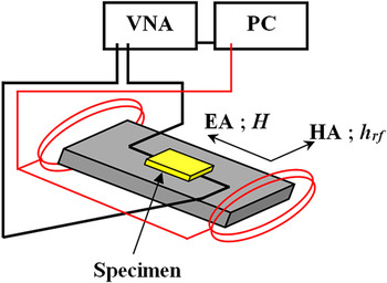
The dynamic parameters were investigated by measuring the FMR at different temperatures. Our dynamic measurement setup consisted of a Vector Network Analyzer (Agilent-E8364C, Santa Clara, CA) equipped with a low-pass filter circuit that excited the sample at high frequency. Figure 1 shows this configuration, where h rf in the frequency range of 1–20 GHz was applied along the HA direction and produced the magnetization precession of the sample, which was mounted upside-down onto the circuit. During the measurements, a varying dc-external magnetic field H was applied along the EA or cooling field direction, and the S-parameters were measured at different dc-fields that exceed the saturation field. Varying the external field allowed the extraction of the dynamic fields. The fast microwave field can avoid thermally activated switching events in the AFM layer. Reference Nogues, Sort, Langlais, Skumryev, Surinach, Munoz and Baro11 For the temperature dependence measurements, the circuit assembly was installed directly onto the cold finger of a probe station chamber (CPX-HF, Lake Shore Cryotronics, Inc., Westerville, OH) which allowed a temperature range of 5–350 K with uncertainty less than 0.2 K. The external field dependence of the resonance frequency was extracted and fitted to the Kittel's equation, as will be explained later, to estimate the effective dynamic magnetic anisotropy field (H eff,dyn), where:
 $${f_{{\rm{res}}}} = {{\rm{\gamma }} \over {2{\rm{\pi }}}}\sqrt {{H_{{\rm{eff,dyn}}}}({H_{{\rm{eff,dyn}}}} + 4{\rm{\pi }}{M_{\rm{S}}})} \quad .$$
Experimental configuration for dynamical measurements. The external magnetic field H is along the EA and the rf magnetic field h rf is along the HA.

Eventually, the rotatable anisotropy H rot was calculated for different AFM layer thicknesses within the whole temperature range.
IV. RESULTS AND DISCUSSION
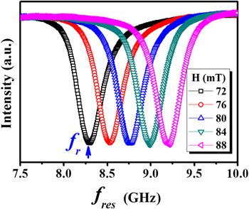
Figure 2 presents one example of our FMR measurements for the sample with t
AFM = 0 nm measured at T = 5 K. Similar FMR spectra were collected for all samples at different temperatures. From these FMR spectra, the resonance frequency (f
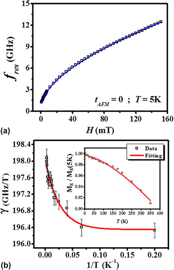
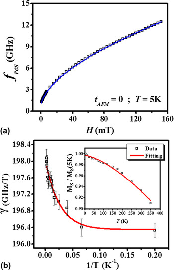
res) can be extracted as a function of the external magnetic field as shown in Fig. 3(a). The effective dynamic magnetic anisotropy field (H
eff,dyn) can be extracted from the fitting of this data to the Kittel's equation [Eq. (4)] assuming H
eff,dyn as a fitting parameter. Since a wide range of values for gyromagnetic ratio γ can be found in the literature,
Reference Stoecklein, Parkin and Scott17,Reference Liu, Wang, Lim, Ng, Kuok, Lockwood, Cottam, Nielsch and Gösele80–Reference Fukumoto, Kuch, Vogel, Camarero, Pizzini, Offi, Pennec, Bonfim, Fontaine and Kirschner85
we treat γ also as a fitting parameter. We fit the saturation magnetization data of our reference sample (t
AFM = 0 nm) acquired from the SQUID measurements to the Bloch’s law, M
S(T) = M
S(0)(1−BT
3/2),
Reference Mathon and Ahmad86,Reference Kittel87
which gives the decay constant B = (1.26 ± 0.03) × 10−5K−3/2 as shown in the inset of Fig. 3(b). As can be seen, there are slight deviations between the experimental data of MS(T) and the fitting curve. This can be essentially attributed to the spin waves
Reference Mathon and Ahmad86,Reference Kittel87
and some experimental errors. When we used the fitted M
S(T) results, the f
res(H) for all represented temperatures of the reference sample can be fitted very well to the Kittel's law. We found that γ increases slightly with temperature or decreases exponentially with the reciprocal of the temperature (1/T) as shown in Fig. 3(b) and it can be fitted very well to an empirical formula
 ${\rm{\gamma }}(T) = {\rm{\gamma }}(0) + A{\rm{e}}^{{{ - C} \mathord{\left/ {\vphantom {{ - C} {k_{\rm{B}} T}}} \right. \kern-\nulldelimiterspace} {k_{\rm{B}} T}}}$
with γ(0) = 196.3 ± 0.11 GHz/T and constant C = (5.4 ± 0.9) × 10−22 J, which is very close to a previously reported value for the interatomic exchange constant (J
NiFe–IrMn = 7.6 × 10⁻²² J) of the NiFe–IrMn coupling.
Reference Xi, Rantschler, Mao, Kief and White88,Reference Tripathy, Adeyeye and Singh89
Assigning the above values to M
S(T) and γ(T), the f
res(H) for all other samples at different measuring temperatures fit well to the Kittel's equation as shown in Fig. 3(a).
FMR measurement spectra under various static external magnetic fields for the reference sample at 5 K.

(a) Field dependence of f res, symbols are the experimental data and solid line is a least square fit to the Kittel’s formula. (b) Temperature dependence of γ with the fitting to our empirical formula, see text. Inset: M S(T) for the reference sample with the fitting to the Bloch's law.
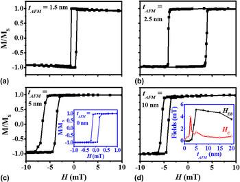
Typical dc hysteresis loops measured at room temperature are shown in Fig. 4. For the reference sample (t AFM = 0 nm), a regular hysteresis loop was obtained with coercivity of <2 Oe along the EA. With t AFM = 1.5 nm, the coercivity along the EA increased without any EB. When t AFM = 2.5 nm, the coercivity continued to increase with the appearance of a small EB. Upon further increase in thickness, the coercivity started to decrease and H EB continued to increase until saturation around t AFM = 5 nm. Beyond this point, H EB slightly decreased with increasing thickness and the coercivity also decreased but maintained a value higher than that of the reference sample. From these results, it can be seen that the onset of EB occurred at AFM critical thickness of ∼2.5 nm and saturated around a thickness of 5 nm, which are slightly higher than the previously reported thicknesses Reference Ali, Marrows, Al-Jawad, Hickey, Misra, Nowak and Usadel74 but are more close to the values reported in Ref. Reference McCord, Mattheis and Elefant77. The AFM layer thickness dependence of both H C and H EB [see the inset of Fig. 4(d)] is common where H C peaks at the onset of H EB. Reference McCord, Kaltofen, Gemming, Hühne and Schultz79
Hysteresis loops along the easy axes of selected samples measured at 300 K, for t AFM = 1.5 nm (a); 2.5 nm (b); 5 nm (c) and 10 nm (d). Inset of (c):M-H loop for the reference sample at 300 K. Inset of (d): t AFM dependence of H C and H EB.

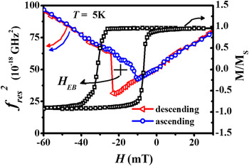
Figure 5 presents a field dependent dynamic hysteresis loop of squared resonance frequency and a static hysteresis loop for the sample with t AFM = 5 nm measured at T = 5 K. Two issues can be observed. First, there is a clear discrepancy between the static and dynamic EB. The dynamic measurements lead to a dynamic EB (H EB,dyn) closer to the coercivity of the ascending half of the static loop. This behavior was explained by assuming that the magnetization reversal along the EA is asymmetric relative to the EB field. Reference McCord, Mattheis and Elefant77 Second, there is asymmetric switching between the descending and ascending parts of both the static and dynamic loops. The hysteresis loop of an isolated FM material is usually symmetric with respect to the field and magnetization axes. In our samples, the unidirectional anisotropy and the stability of the AFM result in asymmetries in the loops. Different origins for this asymmetry can be distinguished from the static loop shape. Since the descending branch of our static loop is more extended as compared with the ascending branch, the asymmetry is more likely related to the concept of a partial domain wall in the AFM. Reference Kim and Stamps90 This mechanism imposes the formation of a parallel domain wall (exchange spring) in the AFM layer and the reversal is understood in terms of domain wall pinning in AFM. Reference Kim and Stamps90,Reference Nikitenko, Gornakov, Shapiro, Shull, Liu, Zhou and Chien91 Pinning of the partial wall occurs during reversal and then during remagnetization, the wall is released from the pinning center at a different field, thus resulting in asymmetry in the hysteresis loop. The energy barrier between wall pinning and release increases with defect concentration, resulting in a larger coercivity and reduced bias. Reference Kim and Stamps90
Squared resonance frequency versus external field measured at T = 5 K for sample with t AFM = 5 nm (left axis) and the EA loop measured under the same condition (right axis). All lines are guides to the eye.

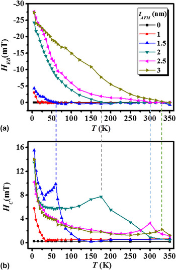
The temperature dependence of EB has been studied extensively. One generally accepted model is the following: at low temperatures, domain walls form in the AFM and remain pinned to the interface as the FM magnetization is reversed. Reference Wee, Stamps and Camley43 At higher temperatures, partial walls in the AFM are depinned during the magnetization reversal of FM and EB disappears at the blocking temperature T B, the temperature above which the static EB vanishes. This behavior can be clearly observed in our samples as shown in Fig. 6, which presents the temperature dependence of H EB and H C for different AFM layer thicknesses. For all presented samples, except that with t AFM = 1 nm which differs in H C behavior, the EB field disappears while H C peaks at T B, then decreases with further increase in temperature, and reaches the coercivity value of the reference sample (t AFM = 0) at some temperature higher than T B. The reference sample's coercivity decreases slightly from its low temperature value of about 2.5 Oe to its room temperature value of about 1.5 Oe. Hence, the behavior of H C(T) for the biased samples is due to the coupling of the FM to the AFM. Similar behavior for H C(T) was reported by different authors, who associated the increased coercivity with the hysteretic losses at this temperature range in the AFM layer. Reference Stiles and McMichael5,Reference Fulcomer and Charap49,Reference Leighton, Fitzsimmons, Hoffmann, Dura, Majrkzak, Lund and Schuller92 Theoretically, this peak of H C was associated with the instabilities in the AFM grains around T B, and even double peaks were observed in simulations. Reference Stiles and McMichael5 Kim et al. proposed that the enhanced coercivity below T B is related to the domain wall pinning at magnetic defects. Reference Kim and Stamps90 The presence of an attractive domain-wall potential in the AFM layer, arising from magnetic impurities, can provide an energy barrier for domain-wall movements that controls coercivity. Ali et al. suggested that enhanced coercivity just above T B could be due to the effect of the AFM layer. Since the AFM layer in its paramagnetic state still experiences an interfacial exchange field originating from the FM and a paramagnet in a field has a magnetization, which must follow the FM during reversal, the H EB is zero but an enhanced H C can still exist. Reference Ali, Marrows, Al-Jawad, Hickey, Misra, Nowak and Usadel74
(a) EB, (b) coercivity as functions of temperature for different t AFM. The dashed lines represent T B.

The AFM thickness dependence of the EB and coercivity (not shown here) shows very similar behaviors to those presented in Ref. Reference Ali, Marrows, Al-Jawad, Hickey, Misra, Nowak and Usadel74 except that our H
EB(t
AFM) peak was suppressed at lower temperature of about 175 K. The peak of H
EB at a specific AFM layer thickness was attributed to the competition between the initial amount of interface magnetization and its stability. The authors therein exclude the possibility of the presence of parallel domains in the AFM layer based on the onset of H
EB at low thicknesses. However, one can roughly estimate the domain-wall thickness using the expression
 ${\rm{\delta }}w = ({\rm{\pi }}/2)\sqrt {{A_{{\rm{AFM}}}}/{K_{{\rm{AFM}}}}}$
, where K
AFM and A
AFM are the anisotropy constant and exchange stiffness, respectively. For IrMn, we found from the literature that KAFM = 5.25 × 10⁶ erg/cm3,
Reference Aley, Fernandez, Kroeger, Lafferty, Agnew, Lu and O’Grady93
and AAFM = 9.78 × 10⁻⁹ erg/cm3,
Reference Ali, Marrows and Hickey94
which give δw ≈ 0.68 nm. Such a value for the domain-wall thickness can eliminate the presence of parallel walls in our thinnest sample with t
AFM = 1 nm but it probably will not affect those in our thicker samples. We believe that these parallel walls are responsible for the increasing energy losses in the AFM layer around T
B which lead to the enhanced coercivity. They could be too far from the interface to pin the FM layer, thus allowing the EB to vanish at T
B while the coercivity continues showing enhancement. At low temperatures, both parallel and perpendicular walls can exist simultaneously. While the parallel walls lead to increasing energy losses and therefore enhanced H
C, the perpendicular walls will efficiently pin the FM spins and produce the loop shift. By increasing the temperature, the thermal fluctuation depins the perpendicular walls at T
B while the parallel walls are still effective since they are energetically favorable. Therefore, the EB is lost at T
B while the coercivity keeps showing increased values. This scenario is supported by the absence of H
C(T) peak in our thinnest sample [see Fig. 6(b)], unlike all thicker samples in our study, and by the observed asymmetric hysteresis loops that imply the formation of planar domain walls in the AFM.
Reference Kim and Stamps90
Now, by further increasing the temperature, H
C will drop at some temperature which may represent a first limit to the Néel temperature (T
N).
Reference Ali, Marrows, Al-Jawad, Hickey, Misra, Nowak and Usadel74
In our analysis, we will assume this temperature as the static Néel temperature (T
N,st). This value strongly depends on the AFM layer thickness, a behavior that must be due to the finite-size effect.
Reference Ambrose and Chien95
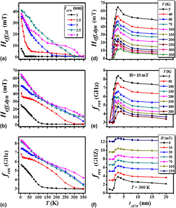
The temperature dependence of the effective static anisotropy field (H eff,st), dynamic effective field (H eff,dyn), and resonance frequency (f res) is presented in Figs. 7(a)–7(c). By increasing the temperature, all these parameters decreased monotonically. However, while H eff,st reached its minimum at the above mentioned T B, both H eff,dyn and f res reached their minima at temperatures higher than T N,st. At these temperatures, the dynamic response of bilayers became the same as our single layer reference sample. This meant that the entire FM/AFM dynamic coupling was destroyed in a similar way to the static case when the coercivities of the bilayers went to that of the reference sample. Therefore, we can assume the temperatures at which H eff,dyn and f res reach their minima as the dynamic Néel temperature T N,dyn. By increasing t AFM, T N,dyn was increased due to the finite-size effect. The difference between the two Néel temperatures can be explained by the rotatable anisotropy field, which is only detectable during the dynamic case due to the short timescale of the FMR measurements. This rotatable anisotropy will add another contribution to the total effective field leading to the enhancement of H eff,dyn and f res and eventually to the enhancement of the dynamic Néel temperature.
Left panel: Temperature dependence of (a) H eff,st, (b) H eff,dyn, and (c) f res for different values of t AFM. Right panel: t AFM dependence of (d) H eff,dyn for different temperatures; (e) f res for different temperatures measured at H = 10 mT; and (f) f res for different external fields measured at T = 300 K.

Another feature is the slight slope change of H eff,dyn(T) at T B. This behavior can be understood as follows: the effective field combines all fields affecting the sample, i.e., anisotropy H eff,st, exchange H EB, rotatable H rot, external H, and demagnetizing fields. Tracking the temperature dependence of the first three fields, we see that while H rot peaks at T B as we will see later, H EB goes to zero and H eff,st to its minimum at this temperature. Therefore, H eff,dyn(T) can change its slope due to vanishing of some contributing fields.
The AFM layer thickness dependence of H eff,dyn and f res is shown in Figs. 7(d)–7(f). At T = 300 K, the onset of H eff,dyn and f res occurred at a critical AFM thickness of about 2 nm, slightly thinner than the onset thickness for the static EB. The different onset between the static and the FMR measurements can also be ascribed to the contribution of the rotatable anisotropy. Reference McCord, Mattheis and Elefant77 We found that both H eff,dyn(t AFM) and f res(t AFM) peak at specific AFM layer thicknesses that depend on the measuring temperature. The peaks occurred at higher thicknesses when the temperature was increased due to the increasing thermal fluctuation. Similar behavior was reported in the static H EB(t AFM) and was suggested to be related to variations in the magnetic structure since that peak was completely suppressed by increasing the temperature to around 200 K. Reference Ali, Marrows, Al-Jawad, Hickey, Misra, Nowak and Usadel74 In our dynamic measurements, the peak strength of H eff,dyn(t AFM) and f res(t AFM) decreased but was not completely suppressed by increasing the temperature up to 350 K (maximum temperature in our system) at moderate external field. The extension of this peak in the dynamic measurements to a higher temperature compared to the static case indicated the crucial role of H rot in this region of AFM thicknesses. At 300 K and above, this peak was almost suppressed by increasing the external fields to 1 kOe or higher as can be seen from Fig. 7(f).
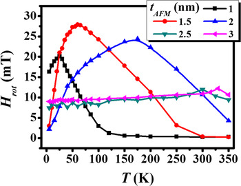
The rotatable anisotropy as a function of the temperature for different AFM layer thicknesses is shown in Fig. 8. It is interesting to see that H rot shows a peak value at the blocking temperature T B. Similar behavior of the rotatable anisotropy versus temperature was expected theoretically from a model calculation, which assumes that the important source of temperature dependence for the system comes from thermal instabilities of the AFM grains. Reference Stiles and McMichael96 By decreasing the temperature, the rotatable anisotropy increases with increasing domain-wall stability until the blocking temperature. Then, as the AFM grains become stable, they start contributing to the unidirectional anisotropy and not to the rotatable anisotropy. Therefore, the rotatable anisotropy starts to decrease. This is also consistent with our results in Fig. 7(a), where H eff,st start to increase significantly below the blocking temperature. In this model, it was assumed that all grains were stable at zero kelvin, and the rotatable anisotropy would go to zero. As can be seen from our experimental results, the rotatable anisotropy does not vanish at the lowest measuring temperature of 5 K, which suggests that the system cannot reach a completely frozen state at which whole AFM grains are stable during the switching of the FM layer magnetization. Instead, we found that H rot will vanish at high temperature, which is consistent with the T N,dyn predicted in our results from the temperature evolutions of H eff,dyn and f res, see Figs. 7(b) and 7(c). At this temperature, the thermal energy becomes large enough to destroy the magnetic ordering of the AFM layer and the whole FM/AFM coupling is certainly lost. Interestingly, we observe that the peak of H rot(T) curve is broadened by increasing the AFM thickness. This can be interpreted as the increase in the AFM grains volume distribution with the AFM layer thickness. Reference Fernandez, Outon and O’Grady97 This distribution broadening will produce a wide range of AFM grain volumes that have different energy minima, different stability temperatures, and eventually different contributions to the measurements. The volume distribution broadening can also explain why the H EB usually decreases after its saturation at the thick AFM layers since the EB is limited to the fraction of grains that are larger than the critical volume to withstand against any thermal activation.
Temperature dependence of the rotatable anisotropy field for different t AFM.

V. CONCLUSIONS
To summarize, we have experimentally studied the EB bilayer system NiFe/IrMn with varying IrMn thickness both statically and dynamically to clarify the effects of temperature and AFM layer thickness on the system’s properties and stability. We found that the static EB vanishes while the coercivity peaks at the blocking temperature. The onset of static EB at room temperature is around 2.5 nm of IrMn. At low temperatures, both H EB and H C increase with increasing t AFM, peak at some thickness, and then decrease. The static measurements suggest the possibility of the presence of both parallel and perpendicular domain walls in the AFM layer. From the dynamic measurements, we found that γ has slight temperature dependence, which should be considered to fit the dynamic resonance frequency to the Kittel's formula. By increasing the temperature, all H eff,dyn, H eff,st, and f res parameters decrease, but as a function of AFM layer thicknesses, these parameters peak at specific t AFM values. Unlike the peaks observed in H EB(t AFM), the H eff,dyn(t AFM) and f res(t AFM) peaks extend to high temperatures and require a strong external field to be suppressed. Our static and dynamic measurements result in different values of the Néel temperatures. All these features can be explained by the contribution of the rotatable anisotropy field. The rotatable anisotropy was also studied at different AFM layer thicknesses and was found to have a peak value at the blocking temperature and approaching zero at the dynamic Néel temperature T N,dyn.
ACKNOWLEDGMENTS
This work was supported by the National Science Council and the Taiwan International Graduate Program, Academia Sinica, Taiwan, Republic of China. The technical help of Christine Lu is appreciated.