1 Introduction
The seminal work of Nikuradse (Reference Nikuradse1930) on turbulent flows in non-circular pipes has highlighted the presence of important large-scale features known as secondary flows. These secondary flows embedded within a primary flow manifest in the form of streamwise vortices. Prandtl (Reference Prandtl1952) showed they can exist in various flow conditions, and classified them into two kinds based on their generation mechanism. The first kind is generated due to mean flow skewness such as in pipe systems with curvatures, whereas the second kind originates from turbulence anisotropy such as in straight non-circular duct flows.
Until the late 1960s, the majority of efforts were directed towards the description and understanding of these two kinds of secondary flows in the presence of smooth surfaces. The introduction of surface roughness was probably first carried out by Hinze (Reference Hinze1967, Reference Hinze1973). Hinze experimentally investigated the turbulent secondary flows in a rectangular duct with a partially corrugated wall, and showed the occurrence of secondary flows both in the corners as well as in the rough-to-smooth spanwise step change. He reported that downwash and upwash motions occurred above the rough and smooth strips, respectively.
Ever since, secondary flows caused by surface roughness have attracted increased consideration owing to their presence in a wide variety of applications. Their presence is ubiquitous in environmental flows such as fluvial processes, where they are often associated with the formation of bedforms and cause variations in topographical sediment distribution (Nezu & Nakagawa Reference Nezu and Nakagawa1984; Colombini Reference Colombini1993; Nezu, Tominaga & Nakagawa Reference Nezu, Tominaga and Nakagawa1993; McLelland et al. Reference McLelland, Ashworth, Best and Livesey1999; Gyr & Kinzelbach Reference Gyr and Kinzelbach2004). In engineering flows, their presence has been observed in ablated turbine blades (Barros & Christensen Reference Barros and Christensen2014), herringbone riblets (Nugroho, Hutchins & Monty Reference Nugroho, Hutchins and Monty2013), superhydrophobic surfaces (Türk et al. Reference Türk, Daschiel, Stroh, Hasegawa and Frohnapfel2014), wind farms (Vanderwel, Placidi & Ganapathisubramani Reference Vanderwel, Placidi and Ganapathisubramani2017) or simply highly ordered roughness (Willingham et al. Reference Willingham, Anderson, Christensen and Barros2014). In almost all of these examples, when the spanwise characteristic wavelength is comparable to the dominant length scale of the flow, large-scale secondary motions occur (Vanderwel & Ganapathisubramani Reference Vanderwel and Ganapathisubramani2015; Yang & Anderson Reference Yang and Anderson2017; Chan et al. Reference Chan, MacDonald, Chung, Hutchins and Ooi2018; Chung, Monty & Hutchins Reference Chung, Monty and Hutchins2018). Therefore, the heterogeneity of the flow over a surface depends entirely on the interaction between the surface and the flow developing over it.
These surfaces can be broadly classified into two categories: (1) surfaces with topographical variation (i.e. adjacent regions of elevations and valleys) and (2) surfaces with skin-friction variation (i.e. alternating high and low shear stress). However, it is unclear as to what surface conditions might result in the skin-friction heterogeneity. It is very likely that ‘roughness’ heterogeneity could lead to this condition. Alternatively, this can be achieved using strips of different drag increasing/decreasing surfaces. All of these different ways have been reported in the literature (Nugroho et al. Reference Nugroho, Hutchins and Monty2013; Barros & Christensen Reference Barros and Christensen2014; Türk et al. Reference Türk, Daschiel, Stroh, Hasegawa and Frohnapfel2014; Willingham et al. Reference Willingham, Anderson, Christensen and Barros2014). Irrespective of their type, similar features can be observed over all heterogeneous surfaces. The secondary motions entail a highly three-dimensional flow, with high- and low-momentum pathways (HMP/downwash and LMP/upwash) alternating in the spanwise direction (Mejia-Alvarez & Christensen Reference Mejia-Alvarez and Christensen2013). The upwash region harbours large-scale low-momentum regions with strong lateral meandering in the outer region, which induces a vertical tilt in the coherent structures between the HMPs and LMPs, enhancing lateral momentum transfer (Kevin et al. Reference Kevin, Monty, Bai, Pathikonda, Nugroho, Barros, Christensen and Hutchins2017; Kevin, Monty & Hutchins Reference Kevin, Monty and Hutchins2019). These regions are accompanied by a strong Reynolds shear stress and turbulent activity which are inhomogeneous in the cross-plane. This induces an imbalance between turbulence production and viscous dissipation, which leads to amplified radial fluctuations that translate into streamwise vorticity (Hinze Reference Hinze1973; Anderson et al. Reference Anderson, Barros, Christensen and Awasthi2015; Hwang & Lee Reference Hwang and Lee2018). However, in spite of their impact on the primary flow, the secondary motions are shown to be relatively weak in comparison to the mean flow. In fact, the secondary flows were demonstrated to be simply the result of superimposition of stronger instantaneous vortices, which only occur in a small fraction of the total time, and are unevenly distributed in the cross-plane (Kevin et al. Reference Kevin, Monty, Bai, Pathikonda, Nugroho, Barros, Christensen and Hutchins2017; Vanderwel et al. Reference Vanderwel, Stroh, Kriegseis, Frohnapfel and Ganapathisubramani2019).
Furthermore, the validity and applicability of established concepts in these flows have been questioned since these concepts were developed for flows over homogeneous roughness. In that regard, the validity of outer-layer similarity hypothesis (Townsend Reference Townsend1976) has been discussed. Prior to the study of Barros & Christensen (Reference Barros and Christensen2014), who highlighted secondary motions in a highly irregular surface roughness, Wu & Christensen (Reference Wu and Christensen2007, Reference Wu and Christensen2010) reported statistical as well as structural similarity in the outer layer. They further investigated the inner-outer interactions over the same surface, and reported the amplitude and frequency modulation to be similar to that of a smooth wall at both the HMPs and LMPs, reinforcing the argument of existence of similarity (Pathikonda & Christensen Reference Pathikonda and Christensen2017). Other studies, on the other hand, reported the absence of outer-layer similarity in the mean flow as well as in the turbulence and spectra, owing to roughness effects which extended farther into the outer layer (Yang & Anderson Reference Yang and Anderson2017; Awasthi & Anderson Reference Awasthi and Anderson2018; Chan et al. Reference Chan, MacDonald, Chung, Hutchins and Ooi2018; Chung et al. Reference Chung, Monty and Hutchins2018; Medjnoun, Vanderwel & Ganapathisubramani Reference Medjnoun, Vanderwel and Ganapathisubramani2018).
Despite the commonalities between these numerous heterogeneous surfaces, several aspects still remain ambiguous. In the case of surfaces with skin-friction heterogeneity, the upwash and downwash motions systematically occurred above the low and high skin friction, respectively (Hinze Reference Hinze1973; McLelland et al. Reference McLelland, Ashworth, Best and Livesey1999; Wang & Cheng Reference Wang and Cheng2005; Türk et al. Reference Türk, Daschiel, Stroh, Hasegawa and Frohnapfel2014; Willingham et al. Reference Willingham, Anderson, Christensen and Barros2014; Stroh et al. Reference Stroh, Hasegawa, Kriegseis and Frohnapfel2016; Chung et al. Reference Chung, Monty and Hutchins2018). For the topographical heterogeneities, several studies reported the upwash and downwash motions to occur above elevated and recessed regions, respectively (Nezu & Nakagawa Reference Nezu and Nakagawa1984; Wang & Cheng Reference Wang and Cheng2006; Vanderwel & Ganapathisubramani Reference Vanderwel and Ganapathisubramani2015; Hwang & Lee Reference Hwang and Lee2018; Medjnoun et al. Reference Medjnoun, Vanderwel and Ganapathisubramani2018). In contrast, the opposite behaviour was shown in other experimental and numerical investigations (Mejia-Alvarez & Christensen Reference Mejia-Alvarez and Christensen2013; Barros & Christensen Reference Barros and Christensen2014; Yang & Anderson Reference Yang and Anderson2017; Awasthi & Anderson Reference Awasthi and Anderson2018). The reasons for this difference remains unclear since the elevated/recessed regions have been thought of as regions of ‘high/low’ roughness. Additionally, in order to identify the surface properties that best characterise the heterogeneity, many researchers performed parametric studies. It has been shown that the spanwise spacing between adjacent ridges/strips is a relevant surface parameter of the heterogeneity (Vanderwel & Ganapathisubramani Reference Vanderwel and Ganapathisubramani2015; Yang & Anderson Reference Yang and Anderson2017; Anderson et al. Reference Anderson, Yang, Shrestha and Awasthi2018; Chan et al. Reference Chan, MacDonald, Chung, Hutchins and Ooi2018; Chung et al. Reference Chung, Monty and Hutchins2018). However, other studies have shown that other surface features exhibited a potential to influence the secondary flows, such as the width of the ‘high’ roughness region or the ‘amount’ of roughness (Willingham et al. Reference Willingham, Anderson, Christensen and Barros2014; Türk et al. Reference Türk, Daschiel, Stroh, Hasegawa and Frohnapfel2014; Stroh et al. Reference Stroh, Hasegawa, Kriegseis and Frohnapfel2016) or the ridge shape and width (Goldstein & Tuan Reference Goldstein and Tuan1998; Wang & Cheng Reference Wang and Cheng2006; Hwang & Lee Reference Hwang and Lee2018). Therefore, it becomes natural to look for answers to some of the following questions: How does one predict the location of the upwash and downwash motions for the topographical heterogeneous surfaces? What are the other relevant length scales that carry the heterogeneity information? Can outer-layer similarity still be satisfied in the presence of secondary flows under certain conditions?
The overarching aim of this work is to document the characteristics of these three-dimensional flows and to address some of the above-mentioned questions. We investigate the flow over a smooth ridge-type heterogeneous surface and assess the effect of the shape and width of the ridges. Oil-film interferometry (OFI) in conjunction with cross-stream stereoscopic particle image velocimetry (SPIV) will enable us to assess the impact of these surfaces on turbulent boundary layer flow. We examine the link between the surface heterogeneity and various other flow quantities, such as local (and span-averaged) skin friction, momentum transport due to turbulent and dispersive stresses, structural similarity as well as boundary layer intermittency. Based on the data, we identify an additional surface parameter that affects the nature of secondary flows. The remainder of the paper is organised in four sections. The experimental methodology is described in § 2. The results and discussion are reported in §§ 3 and 4, respectively, followed by a summary and conclusions in § 5.
2 Experimental methodology
2.1 Facility and surface arrangement
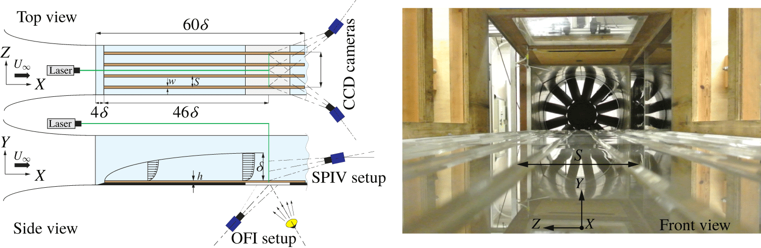
Figure 1 shows the experimental procedure and facility used in the present study. The measurements were carried out in an open-circuit suction wind tunnel at the University of Southampton, in which several rough-wall studies have been documented (Reynolds et al. Reference Reynolds, Hayden, Castro and Robins2007; Vanderwel et al. Reference Vanderwel, Placidi and Ganapathisubramani2017). The extent of the working section is  $0.6~\text{m}\times 0.9~\text{m}\times 4.5~\text{m}$ in
 $(y,z,x)$: wall-normal, spanwise and streamwise directions, respectively. A zero-pressure-gradient turbulent boundary layer grows over a flat surface composed of four equally sized boards, three of which are made of wood to which gloss-PVC plastic sheets are bonded, ensuring a smooth texture. The fourth board made of clear Perspex is used to allow skin-friction measurements using the OFI technique. The boundary layer plates are preceded by a ramp of 0.2 m long inclined by
 $4^{\circ }$ to the horizontal ensuring a smooth transition of the flow from the bottom floor of the test section to the boundary layer plates. The flow is tripped using a 6 mm point-to-point zigzag turbulator tape of 0.5 mm height at 0.26 m downstream of the leading edge of the ramp. Further details of how the wind tunnel was operated can be found in a previous study by Medjnoun et al. (Reference Medjnoun, Vanderwel and Ganapathisubramani2018).
Schematics of the experimental arrangements including the stereoscopic PIV and the OFI set-ups. Both the OFI and the SPIV measurements are performed at a streamwise distance from the leading edge  $x=50\unicode[STIX]{x1D6FF}$, with
 $\unicode[STIX]{x1D6FF}$ being the spanwise-averaged boundary layer thickness at this fetch.

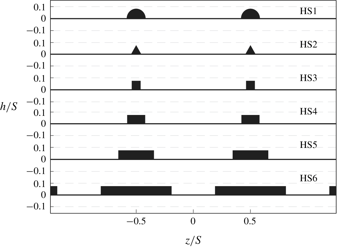
Schematics of the different geometries tested in the present investigation, with the cases HS1, HS2 and HS3 representing the shape effect and HS4, HS5 and HS6 representing the width effect.

Idealised heterogeneous surfaces were created using different profiles of smooth ridges made of clear Perspex (with the same surface texture as the smooth wall). These profiles are selected in order to assess the secondary flow sensitivity to shapes and widths. A semicircle, a triangle and a square are used for the study of the shape effect, while three rectangles with different widths  $W$ are used to investigate the width effect. These surfaces will be referred to by the labels HS1 to HS6 as shown in figure 2. Their maximum heights
 $h$ and spanwise spacings
 $S$ were chosen to match 0.1 and 1 times the spanwise-averaged boundary layer thickness
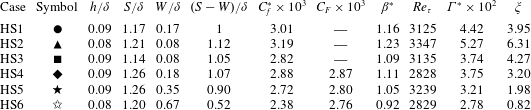
 $\unicode[STIX]{x1D6FF}$, respectively, in order to maximise potential secondary flows (Vanderwel & Ganapathisubramani Reference Vanderwel and Ganapathisubramani2015). Details of the geometrical characteristics of the heterogeneous surfaces are summarised in table 1.
2.2 Oil-film interferometry
The study of wall-bounded flows requires an accurate assessment of the friction velocity, since most of the similarity analysis of the mean and turbulence quantities depends on a knowledge of this scaling parameter. In this study, we measure this quantity using the OFI technique. It is based upon a linear relation between the change in time of the thickness of an oil film deposited on a test surface on top of which a moving air exerts a tangential force, which is represented by the wall shear stress.
Since its introduction by Squire (Reference Squire1961) and its application to a flat wall turbulent boundary layer by Tanner & Blows (Reference Tanner and Blows1976), many researchers have tested the applicability of the OFI technique under several flow conditions. The method has been used in many flows such as adverse-pressure-gradient boundary layers (Pailhas et al. Reference Pailhas, Barricau, Touvet and Perret2009), turbulent boundary layers subjected to free-stream turbulence (Blay Esteban et al. Reference Blay Esteban, Dogan, Rodríguez-Lopéz and Ganapathisubramani2017) and also ‘rough-wall’ boundary layers whose surfaces presented a smooth texture (Akomah, Hangan & Naughton Reference Akomah, Hangan and Naughton2011; Medjnoun et al. Reference Medjnoun, Vanderwel and Ganapathisubramani2018).
Dow Corning 200 silicone oil droplets are deposited at various locations along the spanwise direction to assess the spanwise variation of the skin friction. Their width is less than 0.1 $\unicode[STIX]{x1D6FF}$ such that they are representative of independent skin-friction measurements. Interferograms are obtained by illuminating the droplets using a sodium lamp with a wavelength of 589 nm. A high-resolution LaVision Imager LX 16 MPixel CCD camera with a Nikon 200 mm AF Micro lens set at an angle of
 $25^{\circ }$ from the vertical was fitted to a Scheimpflug adapter to obtain, respectively, a large field of view (FOV) and to satisfy the Scheimpflug condition (shown in the side view of figure 1). A single plane calibration target positioned at the wall in the
 $(x,z)$ plane was used to determine the mapping function through a third-order polynomial fit. This resulted in a FOV of approximately
 $0.6S\times 1.2S$ in the
 $(x,z)$ plane. This allowed the simultaneous capture of the development of different spanwise interferograms. A series of 100 images per surface at four different nominal free-stream speeds (
 $U_{\infty }=10$, 15, 20 and
 $25~\text{m}~\text{s}^{-1}$) are acquired for approximately 10 min in each run using LaVision DAVIS 8.2. The images were subsequently post-processed using a method similar to that described by Blay Esteban et al. (Reference Blay Esteban, Dogan, Rodríguez-Lopéz and Ganapathisubramani2017).
One of the main sources of uncertainty in the OFI technique comes from the oil viscosity (Naughton & Sheplak Reference Naughton and Sheplak2002). Hence, the oil viscosity was calibrated independently of these experiments, using a TA Instruments DHR 3 rheometer for a wide range of temperatures. This allowed a correction of the skin-friction estimates caused by variations in temperature during the measurements. Using a linear uncertainty propagation analysis of the wall-shear-stress equation from the OFI method (see e.g. Pailhas et al. (Reference Pailhas, Barricau, Touvet and Perret2009)), our results highlighted that the leading-order error comes from variations in the oil-film viscosity. In the present study, the overall relative uncertainty in the skin-friction coefficient accounting for both systematic and random sources amounts to 3.1 %. The average deviation of the current results in  $C_{f}$ at matched
 $Re_{\unicode[STIX]{x1D703}}$ (
 $Re_{\unicode[STIX]{x1D703}}=U_{\infty }\unicode[STIX]{x1D703}/\unicode[STIX]{x1D708}$, where
 $\unicode[STIX]{x1D703}$ and
 $\unicode[STIX]{x1D708}$ are the momentum thickness and air kinematic viscosity, respectively) with the smooth-wall correlation of Nagib, Chauhan & Monkewitz (Reference Nagib, Chauhan and Monkewitz2007) is less than 2.5 % (see Medjnoun et al. Reference Medjnoun, Vanderwel and Ganapathisubramani2018).
2.3 Stereoscopic particle image velocimetry
Following observations from previous studies, potential secondary flows are expected to generate a large-scale modification of the turbulent boundary layer leading to strong spanwise heterogeneities. Accordingly, the cross-plane  $(y,z)$ is investigated using SPIV measurements performed at a streamwise location similar to that of the OFI measurements (
 $x=3.2~\text{m}$ downstream the leading edge) as described in the set-up illustrated in figure 1. The flow is traced by vaporised glycerol–water solution particles generated by a Magnum 1200 fog machine, then illuminated with a laser light sheet produced using a two-pulse Litron Nd:YAG laser operating at 200 mJ. A LaVision optical system for the beam focus/expansion of the light sheet is used, comprised of convex and concave lenses in order to focus the beam, and a cylindrical lens in order to expand the sheet with relatively constant thickness in the measurement plane (
 ${\approx}1~\text{mm}$ thickness). The particle images are recorded by two high-resolution LaVision Imager LX 16 MP CCD cameras each fitted with a Nikon 200 mm AF Micro lens and mounted on Scheimpflug adapters to account for the oblique view angle
 $(\pm 42^{\circ })$, and are placed at nearly 1 m from the object plane. A double-sided dual plane calibration target aligned with the laser light sheet was used to determine the mapping function for each camera, using a third-order polynomial fit. This resulted in a FOV of approximately
 $2\unicode[STIX]{x1D6FF}\times 3\unicode[STIX]{x1D6FF}$ in the
 $(y,z)$ plane. Using LaVision DaVis 8.2 software, 3000 statistically independent realisations of image pairs are acquired for each case at 0.6 Hz, with a time delay between two pulses of
 $20~\unicode[STIX]{x03BC}\text{s}$ at a free-stream velocity
 $U_{\infty }=20~\text{m}~\text{s}^{-1}$. This resulted in an average displacement of 7 pixels, which results in roughly 1.5 % bias uncertainty in the measurement (given the sub-pixel uncertainty being around ±0. 1 pixels). The velocity vector fields were subsequently obtained by interrogating particle images using a decreasing multipass scheme starting from window sizes of 48 pixels
 $\times$ 48 pixels to a final pass at 24 pixels
 $\times$ 24 pixels with 50 % overlap. The resulting vector fields were subsequently low-pass filtered at
 $l_{SPIV}^{+}\approx 55$ (with
 $l_{SPIV}^{+}$ being the inner-normalised interrogation window size of the SPIV grid). This prevents the comparison between cases being affected by the grid resolution due to marginal differences in
 $Re_{\unicode[STIX]{x1D70F}}$ (
 $Re_{\unicode[STIX]{x1D70F}}=U_{\unicode[STIX]{x1D70F}}\unicode[STIX]{x1D6FF}/\unicode[STIX]{x1D708}$, where
 $U_{\unicode[STIX]{x1D70F}}$ is the friction velocity).
Geometrical characteristics and aerodynamic parameters for the different heterogeneous surfaces measured at  $Re_{x}\approx 4\times 10^{6}$. The parameters
 $C_{f}^{\ast }$,
 $C_{F}$ and
 $\unicode[STIX]{x1D6FD}^{\ast }$ represent measures of the skin-friction coefficient from OFI measurements and are discussed in § 3.1. The parameters
 $\unicode[STIX]{x1D6E4}^{\ast }$ and
 $\unicode[STIX]{x1D709}$ represent the secondary flow circulation and the surface parameter, respectively, and are discussed in § 3.3. The dimensions of
 $h$ and
 $S$ were fixed to 6 and 80 mm, respectively. The spanwise-averaged boundary layer thickness
 $\unicode[STIX]{x1D6FF}$ was measured by identifying the wall-normal distance at which the spanwise-averaged streamwise velocity reached 99 % of the free-stream speed
 $U_{\infty }$.

3 Results
3.1 The mean viscous drag and flow topology
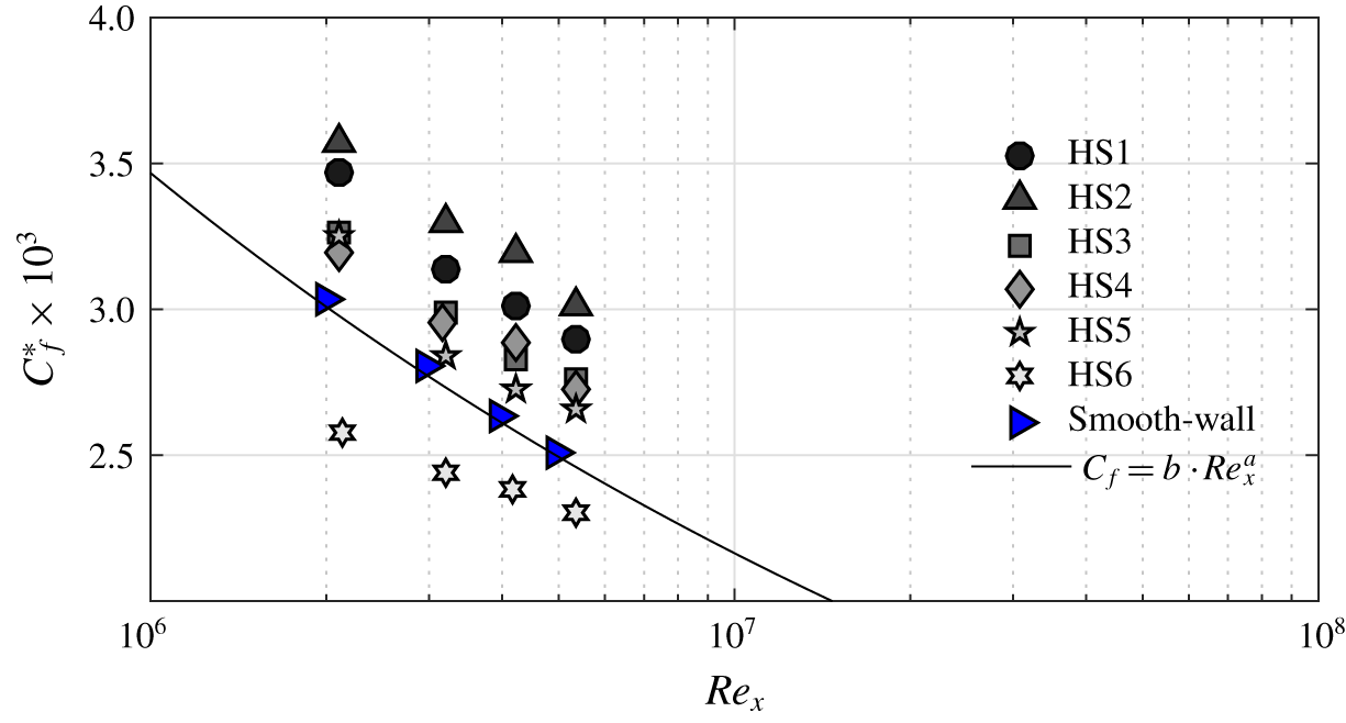
Results from the OFI measurements are presented in figure 3. They describe the response of the surface shear stress to the presence of surface heterogeneity at various moderate Reynolds numbers  $Re_{x}$ (
 $Re_{x}=U_{\infty }x/\unicode[STIX]{x1D708}$, where
 $x$ is the distance to the measurement location from the leading edge) obtained by varying the free-stream speed. We specifically quantify the amount of viscous drag experienced by the wall at the valley, since this information is available for all cases, estimated by
 $$\begin{eqnarray}C_{f}^{\ast }=\langle C_{f}(z_{i})\rangle _{W_{v}},\end{eqnarray}$$
with  $\langle \cdot \rangle _{W_{v}}$ being the spatial average at the valley width (
 $W_{v}=S-W$) across the different discrete points
 $z_{i}$ where the skin-friction coefficient was measured. The results show clearly the decay of the skin friction with respect to Reynolds number. This indicates that regardless of the surface heterogeneity, the flow remains dependent on Reynolds number as opposed to rough-wall turbulence which asymptotes towards a constant value of
 $C_{f}$ at ‘high enough’ Reynolds numbers (Jiménez Reference Jiménez2004; Shockling, Allen & Smits Reference Shockling, Allen and Smits2006; Flack & Schultz Reference Flack and Schultz2014; Djenidi, Talluru & Antonia Reference Djenidi, Talluru and Antonia2018). This can be explained by the fact that these surfaces do not present streamwise rough protrusions which, in addition to viscous drag, lead to pressure drag which causes the fully rough behaviour (Napoli, Armenio & De Marchis Reference Napoli, Armenio and De Marchis2008; Yuan & Piomelli Reference Yuan and Piomelli2014). This observation leads to the hypothesis that these smooth heterogeneous surfaces (as long as their texture is smooth) cannot meet the fully rough conditions, and therefore will always remain dependent on Reynolds number (from the skin-friction perspective). Meanwhile, these results show that the skin-friction coefficient is also dependent on the surface heterogeneity condition. In fact, if we compare the skin-friction coefficients at matched
 $Re_{x}$, we can clearly distinguish that the triangular cross-section case produces more skin friction than the half-round and the square, despite them having the same valley width (
 $(S-W)/\unicode[STIX]{x1D6FF}\approx 1$). This indicates the effect of geometry on the mean streamwise velocity gradient at the wall.
Variation of the valley spanwise-averaged skin-friction coefficient at various moderate Reynolds numbers for the different heterogeneous surfaces. The black solid line represents Schlichting’s power law with  $a\approx -1/5$ and
 $b\approx 0.058$. The blue right-pointing triangles represent the smooth-wall data from Medjnoun et al. (Reference Medjnoun, Vanderwel and Ganapathisubramani2018).

Schlichting’s power-law curve (Schlichting Reference Schlichting1979) is shown to be in good agreement with the present smooth-wall baseline case (compare the solid line against the blue right-pointing triangles in figure 3). The power law further allows quantification of these relative changes against the smooth wall, and are tabulated in table 1 under the label  $\unicode[STIX]{x1D6FD}=(C_{f}^{\ast }/C_{f_{smooth}})$. This quantity represents a measure of the relative drag change at the valley due to the surface heterogeneity. It indicates a net increase in skin friction at the valley for cases HS1 to HS4 (relatively matched valley width
 $(S-W)/\unicode[STIX]{x1D6FF}$), with a
 $23\,\%$ increase for HS2. On the other hand, HS5 and HS6 recorded lower values especially for HS6 which shows local skin-friction reduction. This can be due to the strong viscous blockage induced by the interaction of two boundary layers, one on each of the ridge’s sidewalls. However, if we compare the spanwise-averaged skin-friction coefficient
 $C_{F}$ (also tabulated in table 1), we notice that the overall drag is still higher than that of a smooth wall at an equivalent Reynolds number
 $Re_{x}$. Even though the latter information is not available for the first three cases since the OFI method cannot be applied above the ridges, the expected overall drag should also be higher than that of a smooth wall. From the above results, it is clear that the mean wall shear stress depends on both the geometry of the surface heterogeneity and the Reynolds number. This can be further explored by examining the mean flow using the SPIV data.
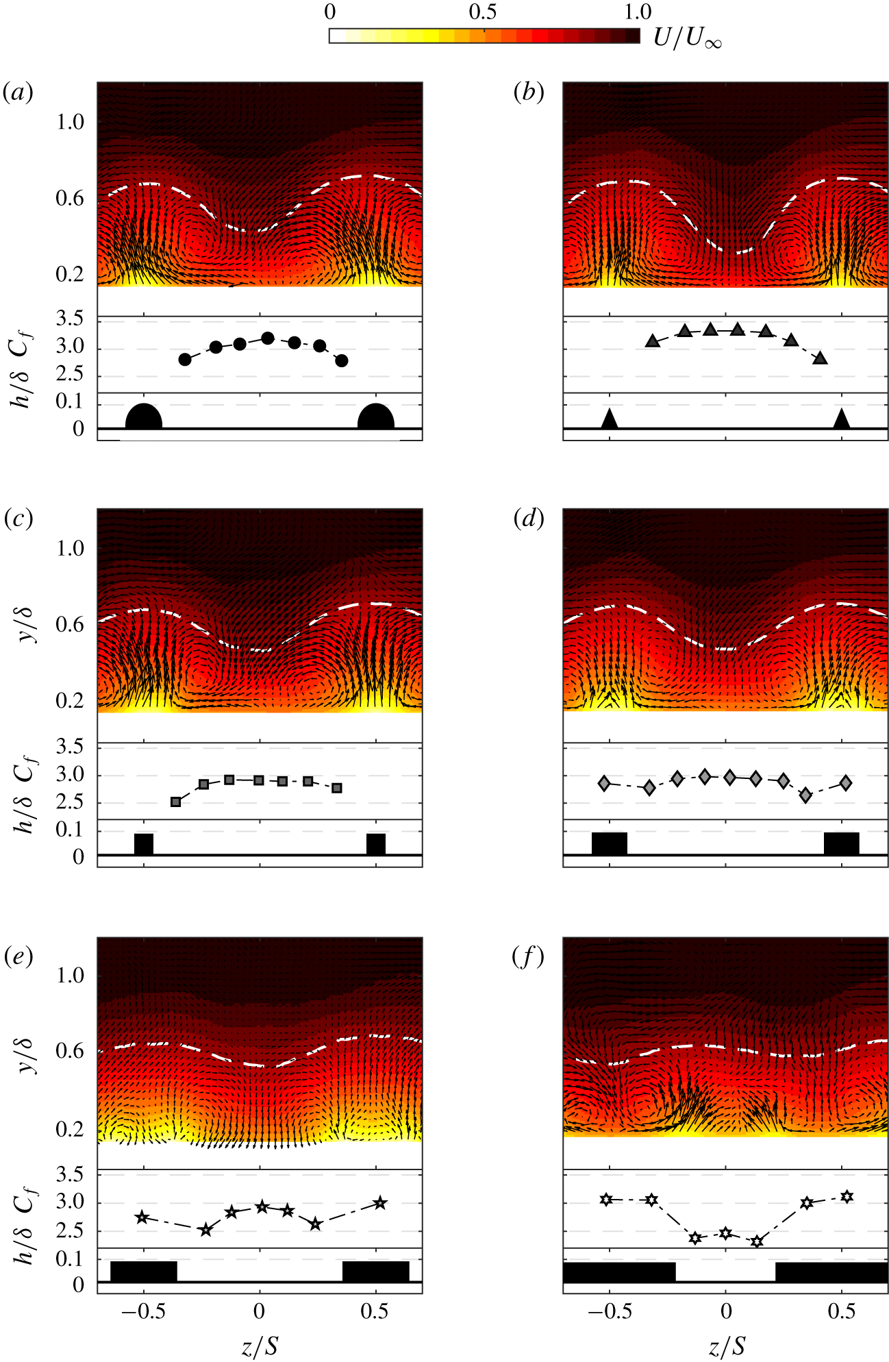
Contour maps of the normalised mean streamwise velocity and the spanwise distribution of the skin-friction coefficient at  $Re_{x}=4\times 10^{6}$: (a) HS1, (b) HS2, (c) HS3, (d) HS4, (e) HS5 and (f) HS6. The cross-sections of the roughness geometries are included at the bottom of the panels to scale for reference. The white dashed line represents the velocity contour level
 $U=0.9U_{\infty }$. The mean in-plane velocity vector plots
 $V$ and
 $W$ are superimposed to highlight the vortical structures.

Figure 4 shows the normalised mean streamwise velocity maps and the spanwise distribution of the skin-friction coefficient, with figure 4(a–c) delineating the shape effect and figure 4(d–f) describing the width effect. Consistent with previous studies, strong spanwise heterogeneities in the mean flow can be distinguished. These are represented in the form of alternating HMPs and LMPs between valleys and peaks, respectively. The degree of spanwise heterogeneity in the mean flow has also impacted the spatial distribution of the skin-friction coefficient, due to the spanwise variation in the mean velocity gradient at the wall. This is in line with our previous experimental study (Medjnoun et al. Reference Medjnoun, Vanderwel and Ganapathisubramani2018) and the direct numerical simulation (DNS) reported by Hwang & Lee (Reference Hwang and Lee2018), which showed the spanwise distribution of the skin friction to strongly vary across the span, especially near the spanwise step change with sharp changes occurring due to the discontinuity (see figure 11 of Hwang & Lee (Reference Hwang and Lee2018)).
Figure 4 also shows relative similarities between the mean velocity maps and the spanwise distribution of  $C_{f}$ for HS1 to HS4. In fact, despite the inability to measure the local skin friction at the peak symmetry plane (
 $z/S$ =
 $\pm$0.5), the shape of
 $C_{f}(z)$ remains reasonably similar except for the change in magnitude. It appears that the maximum skin friction in the valley occurs at its symmetry plane (
 $z/S=0$), which then decreases in the vicinity of the ridge. This observation is also consistent with the DNS results of Hwang & Lee (Reference Hwang and Lee2018) for ridges of smaller widths with large spanwise spacings. The mean flow topology and the corresponding skin-friction distribution presented in figure 4 show a good correlation, especially for cases HS1 to HS4. In fact, regions of constant skin friction are accompanied by a locally homogeneous mean flow (HMP), while regions of high gradient in the skin friction are associated with strong mean flow heterogeneity (LMP and HMP boundaries).
The topology of the mean flow starts to exhibit differences for case HS5 and changes markedly for HS6. The LMPs appear to widen for HS5 above the ridge, while the HMPs are narrower in the valley. This is accompanied by an increase in skin friction above the ridge when compared to HS4, while the average skin friction in the valley decreases compared to HS4. In the case of HS6, the increase of the ridge width has led to a reorganisation of the flow topology, clearly showing a swap in the locations of the HMPs and LMPs. This rearrangement in the mean flow has also impacted the spanwise distribution of the skin-friction coefficient, as higher skin friction is now recorded above the ridge while a reduction in skin friction is observed in the valley, causing a local drag reduction. This can be explained by an increase in the viscous blockage caused by the ridge sidewall boundary layers interacting with one another. This seems to specifically occur when the ridges are made wide enough such that they start influencing the neighbouring ones. It is also of interest to point out that for HS5 and HS6, the degree of spanwise mean flow heterogeneity is lower than that for the other cases. As can be seen from figure 4(e,f), the spanwise variation in the mean velocity contour level  $0.9U_{\infty }$ highlighted with the white dashed line (or the levels seen beyond
 $0.6\unicode[STIX]{x1D6FF}$) is weaker when compared with the rest of the cases.
The results shown in figure 4(a–e) are all in agreement with previous studies that showed the HMPs and LMPs to occur over recessed and elevated regions, respectively (Nezu & Nakagawa Reference Nezu and Nakagawa1984; Colombini Reference Colombini1993; Wang & Cheng Reference Wang and Cheng2006; Vanderwel & Ganapathisubramani Reference Vanderwel and Ganapathisubramani2015; Hwang & Lee Reference Hwang and Lee2018; Medjnoun et al. Reference Medjnoun, Vanderwel and Ganapathisubramani2018). However, the result shown in figure 4(f) seems more to line up with the results of Barros & Christensen (Reference Barros and Christensen2014), Yang & Anderson (Reference Yang and Anderson2017) and Awasthi & Anderson (Reference Awasthi and Anderson2018). These findings indicate that for ridge-type heterogeneous surfaces with  $S/\unicode[STIX]{x1D6FF}\sim O(1)$, both scenarios can occur. Nonetheless, these differences in observations are likely to stem from an additional length scale at play besides
 $S/\unicode[STIX]{x1D6FF}$. This leads us to further question how these observed differences are related to the characteristics of the large-scale secondary flows.
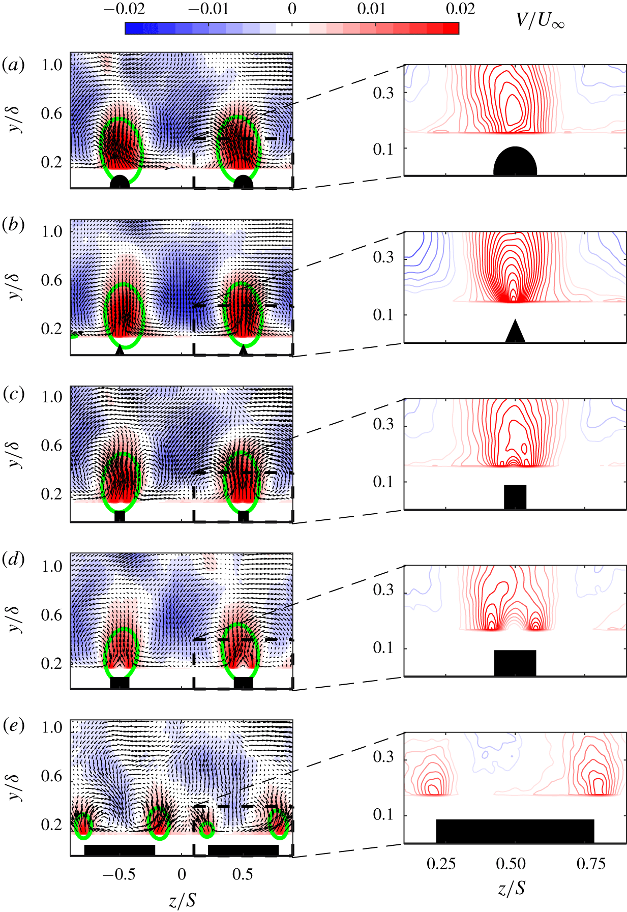
Effect of the roughness geometry on the topology of the mean vertical velocity component (left-hand panel) with a zoom-in of the upwash region (right-hand panel): (a) HS1, (b) HS2, (c) HS3, (d) HS4 and (e) HS6. The mean in-plane velocity vector plots  $V$ and
 $W$ are superimposed to highlight the vortical structures. The green contour level represents
 $V=1\,\%$ of
 $U_{\infty }$.

3.2 Effect on the upwash and downwash of the secondary flows
The effect of surface conditions on the upwash/downwash is shown in the mean wall-normal velocity component in figure 5. This component is of relevance since it directly assesses quantitatively and qualitatively the effect of ridge geometry on the upwash and downwash motions, besides being a constitutive component of the streamwise vorticity. Figure 5 shows the mean wall-normal velocity maps for five cases out of six (HS5 is omitted for brevity) in the left-hand panels, while zoomed-in contour levels of the ridge are presented in the right-hand panels. These maps clearly illustrate the effect of both shape and width on the magnitude and distribution of the upwash/downwash motions. The top three maps (left and right) indicate the presence of three different ways of upwash motions that depend on shape. For HS1, the strongest upwash point seems to occur at about  $2h$, whereas for HS2 and HS3 the strongest upwash points seem to be fixed very close to the ridge corner(s), with similar attributes to that of an external flow over a smooth corner chine (Moinuddin, Joubert & Chong Reference Moinuddin, Joubert and Chong2004).
Figure 5 indicates that both the magnitude and distribution of upwash can be related to the cross-section (curvature) of the ridge. HS2, which shows the most noticeable upwash, has its sidewalls in a configuration that promotes merging of the flow being deflected to make up a strong single upwash region. Whereas the convex nature of the cross-section in HS1 and the presence of a finite width between the two vertical sidewalls of HS3 can create more resistance to the flow which is moving radially towards the centre of the ridge, resulting in a reduction in the strength of the upwash motion. Other studies have also shown that the deflection of the spanwise motions due to the resistance created by the surface elevations is detrimental in the process of secondary flow generation (Goldstein & Tuan Reference Goldstein and Tuan1998; Wang & Cheng Reference Wang and Cheng2006; Hwang & Lee Reference Hwang and Lee2018).
For the width effect cases, we observe that the upwash regions for HS4 and HS6 become more distinct; however, they tend to decrease in strength. This is further emphasised by looking at the ellipsoid at a matched contour level across cases ( $V=1\,\%$ of
 $U_{\infty }$). The contour level seems to encapsulate a larger area for HS1 to HS3, then starts decreasing for wider ridges. This eventually ends up in the formation of two distinct lumps of upwash regions over a single ridge. It follows that these distinct upwash regions start interacting with the neighbouring ones to eventually end up forming a new coherent upwash region, leading to the swap in the LMP and HMP locations observed in figure 4(f). It is also important to point out that if wider ridges were to be used (
 $W_{v}\ll h$), these upwash/downwash motions would essentially die out, as the surface will recover homogeneity. Given the changes observed in the mean wall-normal velocity component due to the different types of ridges, it is essential to also look at how the secondary motions are distributed in these flows.
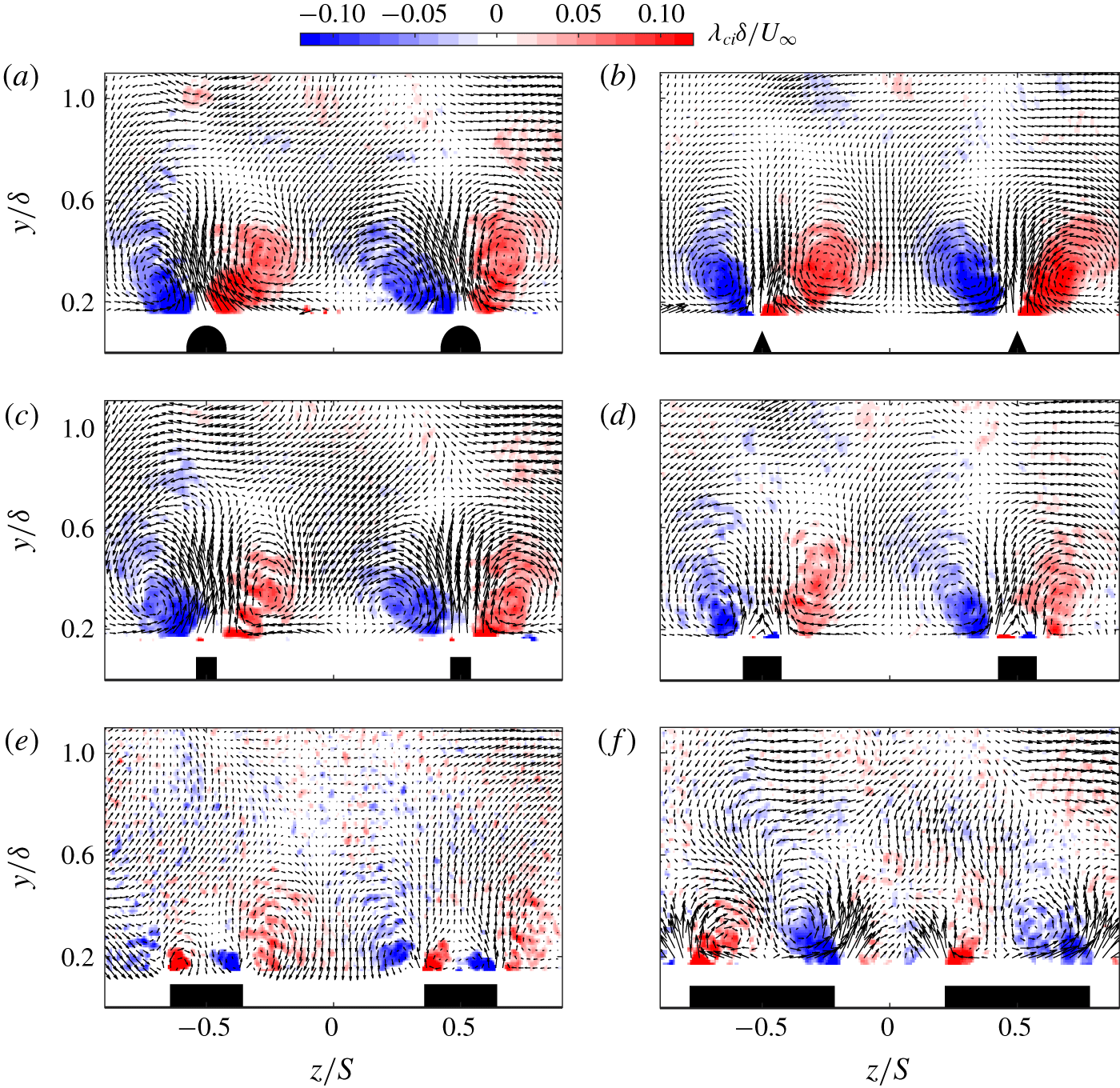
Effect of heterogeneous surfaces on the normalised vorticity-signed swirling strength: (a) HS1, (b) HS2, (c) HS3, (d) HS4, (e) HS5 and (f) HS6. The mean in-plane velocity vector plots  $V$ and
 $W$ are superimposed to highlight the vortical structures on top of the swirling motions.

Following the aforementioned changes observed in the mean flow topology, proportional changes in the generated streamwise vorticity are to be expected. The identification of these streamwise time-averaged vortices was achieved through the determination of the vorticity-signed swirling strength  $\unicode[STIX]{x1D706}_{ci}$. This quantity is expressed as the imaginary part of the complex eigenvalue of the cross-plane velocity gradient tensor, multiplied by the sign of the vorticity in order to identify the rotation sense of the streamwise vorticity (see e.g. Anderson et al. (Reference Anderson, Barros, Christensen and Awasthi2015)). The results are shown in figure 6 and indicate large-scale secondary flows associated with the different heterogeneous surfaces. Consistent with previous studies, these secondary flows consist of a pair of counter-rotating vortices formed on the top of either side of the surface elevations. However, distinctive characteristics are shown across cases, related to both magnitude and distribution of these large-scale vortices. Globally, the spatial extent of
 $\unicode[STIX]{x1D706}_{ci}$ for cases HS1–HS3 is qualitatively similar, although its magnitude seems to be affected by the ridge geometry. However, marked differences are highlighted for cases HS4–HS6. In fact, changes in the streamwise vorticity start to occur; as the ridges become wider for a fixed
 $S/\unicode[STIX]{x1D6FF}$, a pair of new small counter-rotating vortices of opposite sign is visible above the ridges. Similar additional vortices were also observed by Vanderwel & Ganapathisubramani (Reference Vanderwel and Ganapathisubramani2015) but it was speculated that these could have been caused by the presence of small pins on the top of the LEGO brick roughness. However, in a more recent study by Vanderwel et al. (Reference Vanderwel, Stroh, Kriegseis, Frohnapfel and Ganapathisubramani2019) along with the DNS of Hwang & Lee (Reference Hwang and Lee2018), these were reported to exist even for a smooth flat ridge, identical to cases HS4–HS6. The results are similar for both the present experiment and the DNS, and these new structures are shown to grow stronger for wider ridges, while a weakening of the previous large-scale vortices is observed. This feature is believed to also be present for HS3 despite not evident from the map, as it is too small to be captured with the current measurement. Other recent studies also reported these additional streamwise vortices over different surface conditions, terming them tertiary flows to differentiate them from the initial large-scale vortices identified as secondary motions (see e.g. Goldstein & Tuan (Reference Goldstein and Tuan1998), Türk et al. (Reference Türk, Daschiel, Stroh, Hasegawa and Frohnapfel2014), Stroh et al. (Reference Stroh, Hasegawa, Kriegseis and Frohnapfel2016), Benschop & Breugem (Reference Benschop and Breugem2017)). However, it should be noted that according to Prandtl’s definition, any motion occurring in the cross-plane perpendicular to the primary flow should be regarded as a secondary motion/flow. Hence, these different structures can be interpreted as manifestations of different topological states of a secondary flow. In the present description, the terms ‘secondary vortices’ and ‘tertiary vortices’ will be used to identify the previous large-scale (side ridge) and new (above ridge) streamwise vortices.
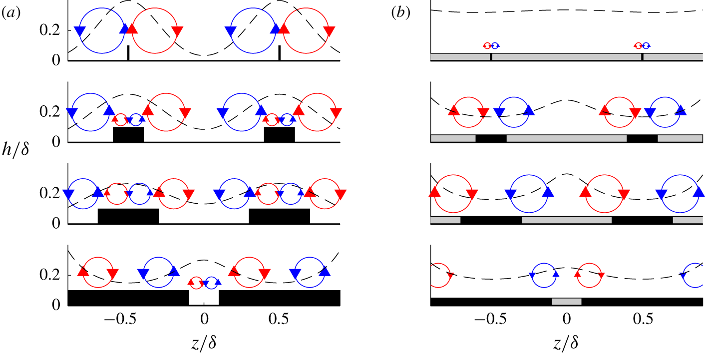
As highlighted in figure 6, these secondary and tertiary vortices are shown to have opposite signs, while their size and to a lesser extent magnitude seem controlled by the valley width  $(S-W)/\unicode[STIX]{x1D6FF}$ (also shown in figures 8 and 9 of Hwang & Lee (Reference Hwang and Lee2018)). It appears that in the vertical direction, the secondary structure propels the low-speed fluid above the ridge away from the wall, and brings the high-speed fluid from the free stream towards the valley. The tertiary structure, on the other hand, attempts to bring the high-speed fluid from the free stream down to the ridge. This is accompanied by a radial motion from the tertiary structure that pushes the low-speed fluid above the ridge towards the valley. Similarly in the spanwise direction, the secondary vortices drive the high-speed fluid from the valley towards the ridges, opposing the tertiary ones. Beyond a given width, the extent of the streamwise vorticity changes due to an imbalance in favour of the tertiary structures which overcomes the secondary vortices. The side ridge secondary vortices continue to weaken leading to the observed swap of the LMP and the HMP locations. At this stage, the tertiary structure becomes the main feature in the cross-plane, resulting in a secondary motion/flow which predominantly produces downwash over the ridges and upwash in between. However, this phenomenon can only take place for spanwise heterogeneous surfaces whose ridges allow the generation of two distinct upwash regions (e.g. rectangular shapes). In fact, it is difficult to imagine this phenomenon occurring for HS1 and HS2 regardless of their widths.
3.3 Relation between the wall shear stress, secondary flows and surface geometry
It is reasonable following the above observations to investigate a potential correlation between the surface heterogeneity, the magnitude of the secondary motions as well as the amount of drag caused by these surfaces. While it can be straightforward to find a metric to quantify the strength of the secondary motions (e.g. cross-flow turbulent kinetic energy or streamwise circulation), it is less clear as to which parameters should be used to characterise the surface geometry. For homogeneous rough surfaces, there are abundant surface parameters in the literature that are used to correlate the surface and aerodynamic properties of the flow (Napoli et al. Reference Napoli, Armenio and De Marchis2008; Flack & Schultz Reference Flack and Schultz2010; Placidi & Ganapathisubramani Reference Placidi and Ganapathisubramani2015; Thakkar, Busse & Sandham Reference Thakkar, Busse and Sandham2017). Whether it is randomly arranged, highly ordered or irregularly distributed roughness, it can have a strong dependence on the amplitude, spacing, density, slope or directionality among other parameters. There is clearly no consensus for a generic formula that will eventually represent all the surfaces.
It has been suggested that for surfaces producing secondary motion, the spanwise wavelength scaled with the dominant length scale of the flow ( $S/\unicode[STIX]{x1D6FF}$) is a good parameter (Vanderwel & Ganapathisubramani Reference Vanderwel and Ganapathisubramani2015; Yang & Anderson Reference Yang and Anderson2017; Chan et al. Reference Chan, MacDonald, Chung, Hutchins and Ooi2018; Chung et al. Reference Chung, Monty and Hutchins2018). It was also argued that for the ridge-type heterogeneous surfaces, the valley width
 $(S-W)/\unicode[STIX]{x1D6FF}$ is important as it can substantially increase or reduce the strength of the secondary motions (Hwang & Lee Reference Hwang and Lee2018). Similarly, for the strip-type heterogeneity, Willingham et al. (Reference Willingham, Anderson, Christensen and Barros2014) have shown that the high roughness width can either increase or decrease the intensity of the upwash/downwash motions by influencing the strength of the transverse mixing. In the present study, most of these scaling parameters would fail to capture the trends exhibited by the secondary flow. In fact, with
 $S/\unicode[STIX]{x1D6FF}$ being constant throughout all the cases,
 $(S-W)/\unicode[STIX]{x1D6FF}$ being constant for cases HS2–HS4 and the effective slope argument being constant for cases HS3–HS6, we need to adopt a different parametrisation since the previous ones cannot adequately represent all these flow changes.
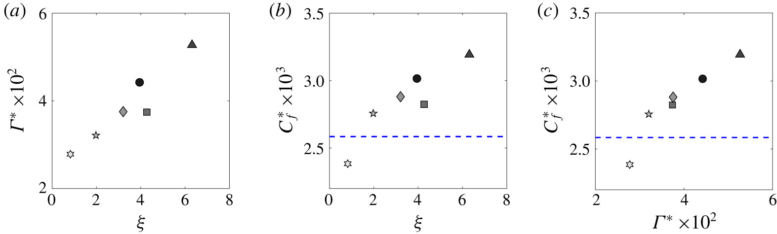
The relations between the strength of these secondary flows and both the surface condition and the spanwise-averaged wall shear stress are presented in figure 7. Figure 7(a,b) quantifies the variation in the streamwise circulation  $\unicode[STIX]{x1D6E4}^{\ast }$ and the skin-friction coefficient
 $C_{f}^{\ast }$ produced by these surfaces at the valley (since this estimate is available for the different test cases) with respect to the surface heterogeneity parameter
 $\unicode[STIX]{x1D709}$. Lastly, figure 7(c) shows the variation of
 $C_{f}^{\ast }$ with respect to
 $\unicode[STIX]{x1D6E4}^{\ast }$. The quantities
 $\unicode[STIX]{x1D6E4}^{\ast }$ and
 $\unicode[STIX]{x1D709}$ which are tabulated in table 1 are defined as

with  $\unicode[STIX]{x1D6E4}^{\ast }=\unicode[STIX]{x1D6E4}/(\unicode[STIX]{x1D6FF}U_{\infty })$ representing the normalised circulation of the streamwise vorticity
 $\unicode[STIX]{x1D6FA}_{x}$. In this study,
 $\unicode[STIX]{x1D6E4}^{\ast }$ essentially quantifies the amount of streamwise vorticity produced in the outer region of the turbulent boundary layer (above
 $0.2\unicode[STIX]{x1D6FF}$). On the other hand,
 $\unicode[STIX]{x1D709}$ represents an attempt to parametrise the surface using a ratio of the recessed (valleys) and elevated (peaks) wetted area. Since the surfaces are streamwise homogeneous, only the perimeters are considered in this study, and are defined as recessed (
 $A_{v}$) and elevated (
 $A_{p}$) areas whenever below or above the mean roughness height
 $\overline{h}$, respectively. As shown in figure 7(a,b), both the amount of streamwise vorticity and frictional drag are affected by these heterogeneous surfaces, despite them having the same
 $S/\unicode[STIX]{x1D6FF}$. This result provides a justification for this surface parametrisation since both the width and the shape of the ridges are captured by
 $\unicode[STIX]{x1D709}$.
In figure 7(a), the streamwise circulation is shown to vary almost linearly within the range of  $\unicode[STIX]{x1D709}$ tested herein. If we consider the asymptotic limits of
 $\unicode[STIX]{x1D709}$, two behaviours are expected to take place. (i) For
 $\unicode[STIX]{x1D709}\rightarrow 0$, the secondary flows are expected to be small enough such that they are confined in the roughness sublayer and the flow will essentially recover homogeneity in the mean and turbulent sense (
 $\unicode[STIX]{x1D6E4}^{\ast }\rightarrow 0$). This is the limit where the surface is homogeneous. (ii) For
 $\unicode[STIX]{x1D709}\rightarrow \infty$, this can be thought of as a transitional surface that will result in localised but large secondary flows over/near the ridges, while farther away from them the flow is expected to remain homogeneous. In this case, the integrated circulation
 $\unicode[STIX]{x1D6E4}^{\ast }\rightarrow \unicode[STIX]{x1D6E4}_{\infty }^{\ast }$. Between these two limits, a third region can be identified as
 $a<\unicode[STIX]{x1D709}<b$, where
 $a$ and
 $b$ represent the lower and upper limits. This region translates to a strongly heterogeneous flow regime with possible topological bifurcations of the streamwise rollers, with the occurrence of tertiary or even quaternary structures depending on the ridge geometry (Hwang & Lee Reference Hwang and Lee2018). This results in a highly three-dimensional flow which leads to the observed increased circulation
 $\unicode[STIX]{x1D6E4}^{\ast }$ and drag. These observations are also in line with the study carried out by Yang & Anderson (Reference Yang and Anderson2017), which provided similar evidence using a comprehensive range of values of the ridge spanwise spacing normalised with the channel half-height. Their large-eddy simulation results revealed that the spanwise spacing scaling indicates when the flow is expected to become homogeneous, heterogeneous or transitional, supporting the idea of the existence of three distinct regimes. In their study, these bands were termed roughness, intermediate and topography for homogeneous, heterogeneous and transitional, respectively. Similar observations have also been made clear for the alternating high and low shear-stress heterogeneity with the recent DNS of Chung et al. (Reference Chung, Monty and Hutchins2018).
Furthermore, figure 7(b) shows that the local (valley spanwise-averaged) drag increases with increasing  $\unicode[STIX]{x1D709}$. While a drag reduction is observed for HS6,
 $C_{f}^{\ast }$ increases albeit with a lower rate with increasing
 $\unicode[STIX]{x1D709}$. For
 $\unicode[STIX]{x1D709}\rightarrow 0$, the valley skin friction
 $C_{f}^{\ast }$ is naturally expected to tend to
 $0$. However, if we considered the total drag
 $C_{F}$, it might be similar to the homogeneous case (or higher), which in this case is highlighted by the blue dashed line. It is interesting to note that it might be possible to find a surface geometry that leads to an optimal secondary flow condition that would reduce the spanwise-averaged wall shear stress. Further studies are necessary to examine the feasibility of such surfaces, which is beyond the scope of the present work. If
 $\unicode[STIX]{x1D709}\rightarrow \infty$, the skin friction is also expected to return to that of the homogeneous case at some point since the secondary motions will be significantly localised. However, how/when this would happen is also open for further exploration. Overall, we observe that changes in streamwise circulation induce proportional changes in the wall shear stress as demonstrated in figure 7(c) (and vice versa). It essentially reveals that a possible linearity can exist for strong/large secondary flow cases, with an increase in the streamwise circulation leading to a proportional increase in the wall shear stress.
Variation of (a) the normalised compensated circulation  $\unicode[STIX]{x1D6E4}^{\ast }$ and (b) the valley spanwise-averaged skin-friction coefficient with respect to the surface parameter
 $\unicode[STIX]{x1D709}$. (c) The effect of the secondary flow circulation on the drag experienced at the valley. The blue dashed line represents the smooth-wall skin-friction coefficient at an equivalent
 $Re_{x}$. See table 1 for the definitions of the symbols.

3.4 Effect of surface heterogeneity on the turbulence properties
The impact of the surface heterogeneity on the turbulence organisation is further analysed using a triple decomposition performed on the three-component velocity vector in the cross-plane. This concept has been well documented and widely used to assess flows presenting spatial inhomogeneities (Reynolds & Hussain Reference Reynolds and Hussain1972; Raupach & Shaw Reference Raupach and Shaw1982; Nikora et al. Reference Nikora, McEwan, McLean, Coleman, Pokrajac and Walters2007). In this framework, the velocity field can be expressed as
 $$\begin{eqnarray}u_{i}(y,z,t)=U(y)+\tilde{u} (y,z)+u(y,z,t),\end{eqnarray}$$
where  $u_{i}$ is the instantaneous velocity field measured at a given streamwise location,
 $U(y)$ is the spatial- and time-averaged velocity profile,
 $\tilde{u} (y,z)$ is the spatial deviation field independent of time and
 $u(y,z,t)$ is the time-fluctuating part from the Reynolds double decomposition. This decomposition allows us to quantify the amount of stresses arising from the mean flow heterogeneity, which contribute to the total stresses as form-induced (dispersive) stresses. In the case of strong spatial heterogeneities, these dispersive stresses can play a major role in the transport of momentum flux, which can have an impact on the organisation of the turbulent boundary layer structure (Türk et al. Reference Türk, Daschiel, Stroh, Hasegawa and Frohnapfel2014; Meyers, Ganapathisubramani & Cal Reference Meyers, Ganapathisubramani and Cal2019).
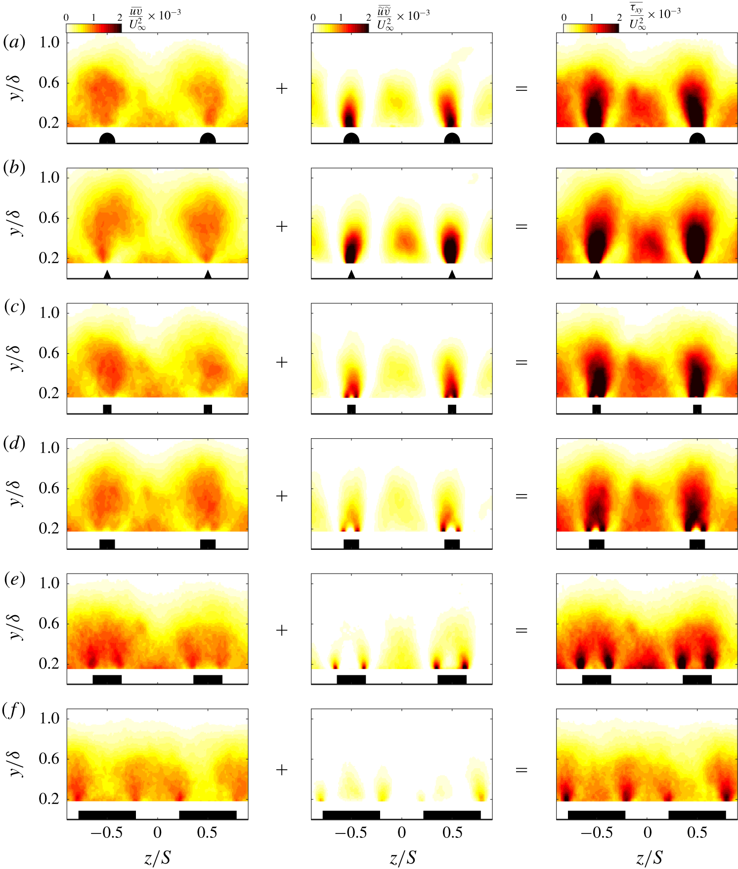
Comparative maps of the turbulent, dispersive and total shear stresses denoted  $\overline{uv}$,
 $\overline{\tilde{u} \tilde{v}}$ and
 $\overline{\unicode[STIX]{x1D70F}_{xy}}$, respectively, are presented in figure 8 (in columns), for different cases (in rows). As expected, the dispersive stresses are not negligible with respect to the turbulent ones. In fact, they appear to be non-zero for nearly two-thirds of the extent of the boundary layer thickness with varying intensity along the spanwise direction (shown in the second column from the left of figure 8). The patterns of the turbulent and dispersive shear stresses do not show particular resemblance. In fact, while the overall distribution of
 $\overline{uv}$ seems to follow a similar wavy character to the mean flow,
 $\overline{\tilde{u} \tilde{v}}$ on the other hand appears to be more localised. The dispersive shear stress is shown to have high intensity above the surface elevation (especially near the ridge edges) as opposed to a weaker magnitude recorded at the valley. Away from the ridges,
 $\overline{\tilde{u} \tilde{v}}$ is shown to span nearly half of the valley extent with highest intensities being recorded at nearly
 $0.3\unicode[STIX]{x1D6FF}$ from the wall. Nevertheless, the dispersive shear stress is shown to vanish between the peaks and valleys, whose regions are characterised by enhanced spanwise and weak wall-normal motions. These observations appear to mainly apply for cases HS1–HS4. This is in contrast with HS5 and HS6, which were shown previously to be the least heterogeneous cases. As illustrated in the middle panels of figure 8(e,f),
 $\overline{\tilde{u} \tilde{v}}$ is observed to reduce in spatial extent and strength, where only a smaller dispersive shear stress remains above the ridges especially for HS6.
For  $\overline{uv}$, a weaker magnitude of the stress is observed at the valley in comparison to the ridge, with an overall distribution being modulated similarly to the mean flow. However, this magnitude is expected to increase when approaching the near-wall region below the currently measured FOV, especially in the vicinity of the centre of the valley. We can also observe from figure 8 that despite the different ridge geometries for cases HS1–HS4, the turbulent shear stress remains globally similar between cases. This observation can perhaps be explained by the fact that once these large-scale secondary motions are formed, changes in surface heterogeneities result only in variations of their strength, without necessarily affecting their spatial extent. This mostly leads to an increased dispersive component, while the turbulent shear stresses remain relatively unchanged. However, this is believed to be only valid when a strong degree of heterogeneity exists. This is further substantiated from the total shear-stress maps
 $\overline{\unicode[STIX]{x1D70F}_{xy}}$ shown in the left-hand column of figure 8. They mainly show that for large-scale secondary flows, their resulting total stresses remain relatively unchanged and their increase in strength will only result in the increase of magnitude of
 $\overline{\unicode[STIX]{x1D70F}_{xy}}$, without necessarily affecting its spatial distribution. These results are also true for the streamwise stress component which was left out for brevity.
Effect of different heterogeneous surfaces on the normalised turbulent (left-hand panels), dispersive (middle panels) and total (right-hand panels) shear stress: (a) HS1, (b) HS2, (c) HS3, (d) HS4, (e) HS5 and (f) HS6.

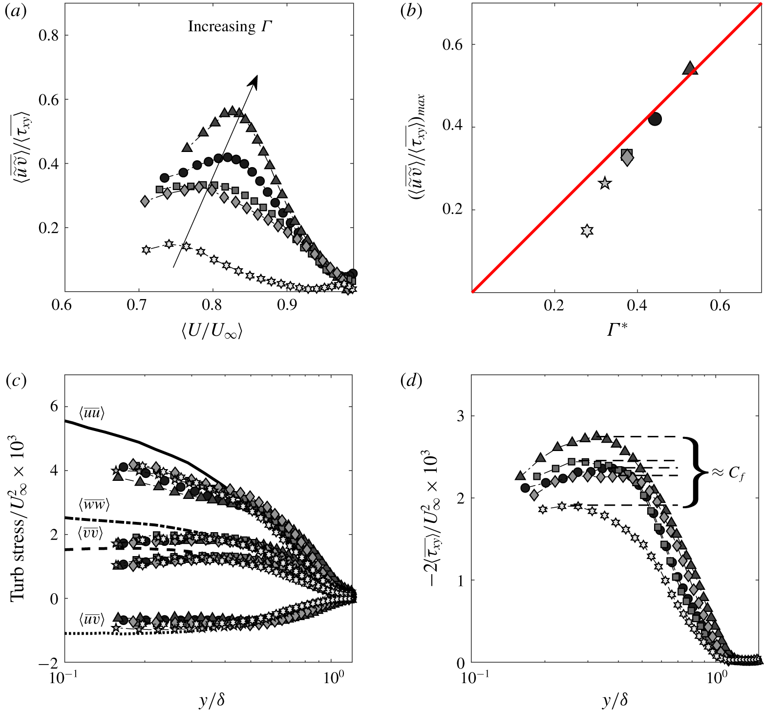
(a) Variation of the dispersive contribution to the total shear stress in the diagnostic form. (b) Variation of the peak of the dispersive contribution normalised with the total shear stress with respect to the secondary flow circulation, with the red solid line representing a  $45^{\circ }$ slope. (c) Variation of the turbulent shear and normal stresses and comparison with their smooth-wall equivalent profiles, with
 $\langle \overline{uu}\rangle$ (solid line),
 $\langle \overline{vv}\rangle$ (dashed line),
 $\langle \overline{vv}\rangle$ (dashed-dotted line) and
 $\langle \overline{uv}\rangle$ (dotted line) taken from the smooth turbulent boundary layer data of Kevin et al. (Reference Kevin, Monty, Bai, Pathikonda, Nugroho, Barros, Christensen and Hutchins2017) with
 $Re_{\unicode[STIX]{x1D70F}}\approx 2500$. (d) Wall-normal distribution of the normalised total shear-stress profiles. See table 1 for definitions of the symbols.

The global behaviour of the dispersive shear stress is further examined using spanwise-averaging over a wavelength. This represents a quantification of the overall effect of the flow heterogeneity on the turbulent boundary layer. The contributions of the dispersive shear stresses to total stress are emphasised in figure 9(a), plotted in the diagnostic form ( $\langle U/U_{\infty }\rangle$). Figure 9(b) highlights the variation of the peak of
 $\langle \overline{\tilde{u} \tilde{v}}\rangle /\langle \overline{\unicode[STIX]{x1D70F}_{xy}}\rangle$ with respect to the streamwise circulation
 $\unicode[STIX]{x1D6E4}^{\ast }$. Figure 9(c), on the other hand, illustrates the spanwise-averaged turbulent normal- and shear-stress distributions compared with their corresponding smooth-wall profiles, while figure 9(d) highlights the wall-normal distribution of the spanwise-averaged total shear stress defined as
 $$\begin{eqnarray}\underbrace{\langle \overline{\unicode[STIX]{x1D70F}_{xy}}\rangle }_{\substack{ total \\ shear \\ stress}}=\underbrace{\unicode[STIX]{x1D708}\frac{\unicode[STIX]{x2202}\langle U\rangle }{\unicode[STIX]{x2202}y}}_{\substack{ viscous \\ shear \\ stress}}-\underbrace{\langle \overline{uv}\rangle }_{\substack{ turbulent \\ shear \\ stress}}-\underbrace{\langle \overline{\tilde{u} \tilde{v}}\rangle }_{\substack{ dispersive \\ shear \\ stress}},\end{eqnarray}$$
which typically accounts for viscous, turbulent and dispersive shear-stress contributions. As observed from figure 9(a), the dispersive stresses are shown to be significant in magnitude for a large extent of the boundary layer thickness. As opposed to classical homogeneous roughness where it is expected to see their contributions to be only important below the canopy, their effect is presently shown to be substantial even in the outer layer. In fact, these form-induced stresses contribute from  $15\,\%$ up to
 $55\,\%$ of the total shear stress for the most heterogeneous case. It is additionally shown that at a given distance from the wall (
 $\langle U/U_{\infty }\rangle =0.9$ or
 $y=0.6\unicode[STIX]{x1D6FF}$), the dispersive stresses have nearly similar decay rates (specifically cases HS1–HS4). This can be interpreted as a result of saturation in size of these large-scale secondary motions for a range of
 $a<\unicode[STIX]{x1D709}<b$, whereby small changes in
 $\unicode[STIX]{x1D709}$ only enhance or weaken the strength of these secondary motions without necessarily affecting their spatial extent. This further supports the results shown in figures 6 and 7 for HS1–HS4, which can be considered to be in a ‘fully’ grown heterogeneous regime. As opposed to HS5 and HS6, they were shown to have both weaker and smaller secondary flows, hence their small impact on the primary flow.
Figure 9(a) also underlines that the maximum peak in  $\langle \overline{\tilde{u} \tilde{v}}\rangle /\langle \overline{\unicode[STIX]{x1D70F}_{xy}}\rangle$ increases both in magnitude and relative height (expressed by
 $\langle U/U_{\infty }\rangle$) when increasing the streamwise circulation; however, the peak remains constant when plotted in
 $y/\unicode[STIX]{x1D6FF}$. This means that the location of the secondary flows remains unaffected, and the increase in circulation only results in a larger mixing causing a fuller turbulent boundary layer flow. In figure 9(b), the variation of
 $\langle \overline{\tilde{u} \tilde{v}}\rangle /\langle \overline{\unicode[STIX]{x1D70F}_{xy}}\rangle _{max}$ with respect to
 $\unicode[STIX]{x1D6E4}^{\ast }$ is emphasised, and is shown to rapidly increase for HS5 and HS6 while almost linearly varying for HS1 to HS4. This result provides further support to the previous interpretation, that the secondary flow formation can undergo different regimes.
The turbulent stresses, on the other hand, are shown in figure 9(c). The turbulent normal stresses  $\langle \overline{uu}\rangle$,
 $\langle \overline{vv}\rangle$ and
 $\langle \overline{ww}\rangle$ as well as the turbulent shear stress
 $\langle \overline{uv}\rangle$ seem to have smaller magnitudes in comparison with their equivalent smooth-wall profiles, for
 $y/\unicode[STIX]{x1D6FF}<0.5$. Moreover,
 $\langle \overline{uu}\rangle$ and
 $\langle \overline{uv}\rangle$ in particular are shown to be affected by the degree of the heterogeneity, with the stronger the secondary motions, the weaker these turbulent stresses become, highlighting lack of collapse between cases. Beyond
 $0.5\unicode[STIX]{x1D6FF}$, a weak degree of collapse is observed; however, this is only valid when scaled by
 $U_{\infty }^{2}$. In fact, when scaled by
 $U_{\unicode[STIX]{x1D70F}}^{2}$ the profiles recover similarity only at the edge of the boundary layer thickness.
Figure 9(d) illustrates the variation of the total shear stress computed using (3.4). The results indicate that overall, the plateau extent and magnitude have been affected by the presence of these large-scale secondary flows. As expected, the magnitude of the plateau increases with increasing  $\unicode[STIX]{x1D6E4}^{\ast }$, which translates to higher wall drag experienced by the surface. Surprisingly, the plateau extent shortens for large
 $\unicode[STIX]{x1D6E4}^{\ast }$ and lengthens for smaller
 $\unicode[STIX]{x1D6E4}^{\ast }$. This behaviour is caused by the dispersive stress contributions which are amplified by these large-scale secondary flows. In fact, this is more evident when comparing the turbulent shear-stress maps to the dispersive ones as shown in figure 8. The dispersive stress contributions seem to be accentuated near the core of the secondary flows (
 $y\approx 0.3\unicode[STIX]{x1D6FF}$), while diminished closer to the wall, leading to the presence of the observed peak in figure 9(a). The turbulent stresses, on the other hand, shown in figure 9(c) seem to have a nearly constant contribution up to
 $50\,\%$ of the boundary layer thickness when spanwise-averaged. Therefore, the presence of a peak instead of a classical plateau in
 $\langle \overline{\unicode[STIX]{x1D70F}_{xy}}\rangle$ is considered to be a consequence of the increased lateral motions which enhance the secondary flows and lead to higher momentum transport. These results are also in agreement with recent studies that assessed the contributions of the dispersive stresses (Chan et al. Reference Chan, MacDonald, Chung, Hutchins and Ooi2018; Meyers et al. Reference Meyers, Ganapathisubramani and Cal2019; Vanderwel et al. Reference Vanderwel, Stroh, Kriegseis, Frohnapfel and Ganapathisubramani2019). They found that these form-induced stresses are prominent within the canopy but can markedly increase spatially depending on the surface heterogeneity length scale. For a certain range of spanwise wavelengths, the turbulent stresses are shown to exhibit strong spanwise gradients which lead to the added dispersive stresses that can extend up to two-thirds of the flow.
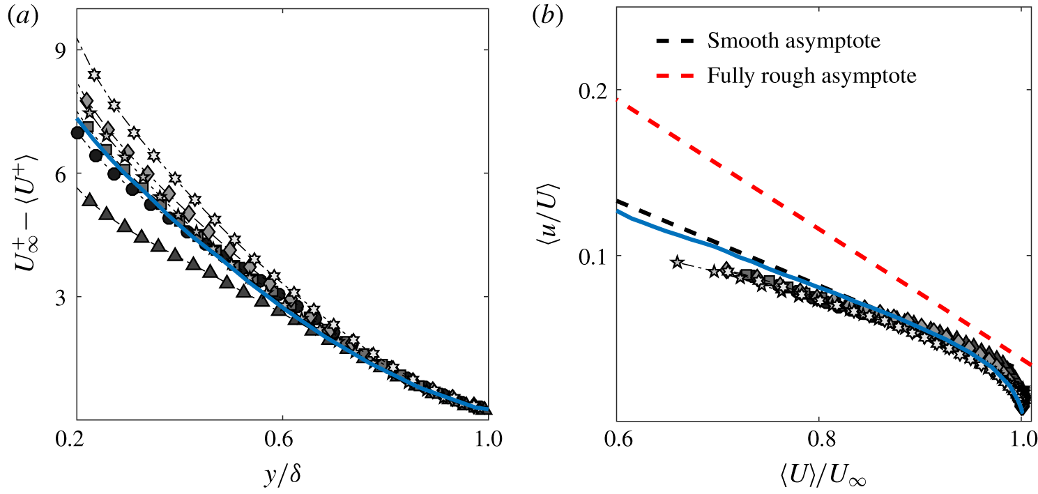
The impact of the secondary flows on the outer-layer similarity is examined in figure 10. Figure 10(a) shows the spanwise-averaged mean velocity profiles in defect form scaled with the friction velocity taken from the total shear-stress plateau. On the other hand, figure 10(b) highlights the spanwise-averaged streamwise turbulence intensity profiles plotted in the diagnostic form introduced by Alfredsson, Segalini & Örlü (Reference Alfredsson, Segalini and Örlü2011). There is marginal lack of collapse in the velocity deficit for all the different surfaces when compared to the smooth-wall data. The absence of collapse extends up to  $y=0.6\unicode[STIX]{x1D6FF}$, whose recovery seems to occur when the dispersive stresses decay faster as shown in figure 8. The turbulence intensity profiles are even more affected by the presence of these large secondary motions, with a recovery only occurring at the edge of the boundary layer (not shown here for brevity). The above observations are consistent with previous results from both ridge-type and roughness-type studies of Chan et al. (Reference Chan, MacDonald, Chung, Hutchins and Ooi2018) and Chung et al. (Reference Chung, Monty and Hutchins2018), respectively. They essentially showed that for spanwise wavelengths comparable to the dominant length scale of the flow, the secondary flows occupy a large portion of the primary flow, leading to strong dispersive stresses (extended roughness sublayer) which results in the breakdown of both global and local outer-layer similarity.
A good collapse is observed for the variance profiles as shown in figure 10(b), not only between the cases, but also with the smooth wall. This suggest that regardless of the changes in the secondary flow circulation, the streamwise turbulence intensity along with the mean flow change proportionally in the outer region. Moreover, the collapse of the profiles with the smooth wall irrespective of a non-zero roughness function  $\unicode[STIX]{x0394}U^{+}$ (representative of the drag changes shown in figure 3) does not seem to be captured in the diagnostic plot. This observation is somewhat inconsistent with the conclusions of Castro, Segalini & Alfredsson (Reference Castro, Segalini and Alfredsson2013) who demonstrated that increasing
 $\unicode[STIX]{x0394}U^{+}$ leads to a higher slope in
 $u/U$ until reaching the fully rough trend (represented by the red dashed line in figure 10b). One possible reason for the current behaviour is that the value of the roughness function is small (
 $\unicode[STIX]{x0394}U^{+}\leqslant 4$). Additionally as discussed in § 3.1, the absence of form drag contribution to
 $\unicode[STIX]{x0394}U^{+}$ due to lack of streamwise rough protrusions can inhibit the increase of the streamwise turbulence level relative to the mean flow. Similar results were also reported in our previous study regarding local profiles across the spanwise direction (Medjnoun et al. Reference Medjnoun, Vanderwel and Ganapathisubramani2018).
Effect of different heterogeneous surfaces on (a) spanwise-averaged mean velocity profiles in the defect form normalised with the friction velocity determined from the total shear stress. (b) Outer scaling of spanwise-averaged streamwise turbulence intensity in the diagnostic-plot form. The blue solid line represents the smooth-wall data from Medjnoun et al. (Reference Medjnoun, Vanderwel and Ganapathisubramani2018). See table 1 for definitions of the symbols.

3.5 Effect on the coherent structures in the outer region
To further investigate the influence of the surface heterogeneity on the characteristics of the turbulence structures, the two-point correlation function of the velocity fluctuations is examined. This allows qualitative and quantitative characterisation of the spatial structures at different critical locations such as the HMPs and LMPs that characterise this flow (Wu & Christensen Reference Wu and Christensen2010; Yang & Anderson Reference Yang and Anderson2017; Bai et al. Reference Bai, Kevin, Hutchins and Monty2018; Kevin et al. Reference Kevin, Monty and Hutchins2019). The two-point correlation coefficient tensor  $\unicode[STIX]{x1D619}_{u_{i}u_{j}}$ in the
 $(y,z)$ plane is defined as
 $$\begin{eqnarray}\unicode[STIX]{x1D619}_{u_{i}u_{j}}(y_{ref},z_{ref})=\frac{\overline{u_{i}(y_{ref},z_{ref})u_{j}(y,z)}}{\unicode[STIX]{x1D70E}_{u_{i}}(y_{ref},z_{ref})\unicode[STIX]{x1D70E}_{u_{j}}(y,z)},\end{eqnarray}$$
where  $y_{ref}$ and
 $z_{ref}$ are the reference wall-normal and spanwise locations at which the correlation is examined. Here
 $\unicode[STIX]{x1D70E}_{u_{i}}(y_{ref},z_{ref})$ is the standard deviation of
 $u_{i}$ at
 $y_{ref}$ and
 $z_{ref}$ and
 $\unicode[STIX]{x1D70E}_{u_{j}}(y,z)$ is the standard deviation of
 $u_{j}$ in the
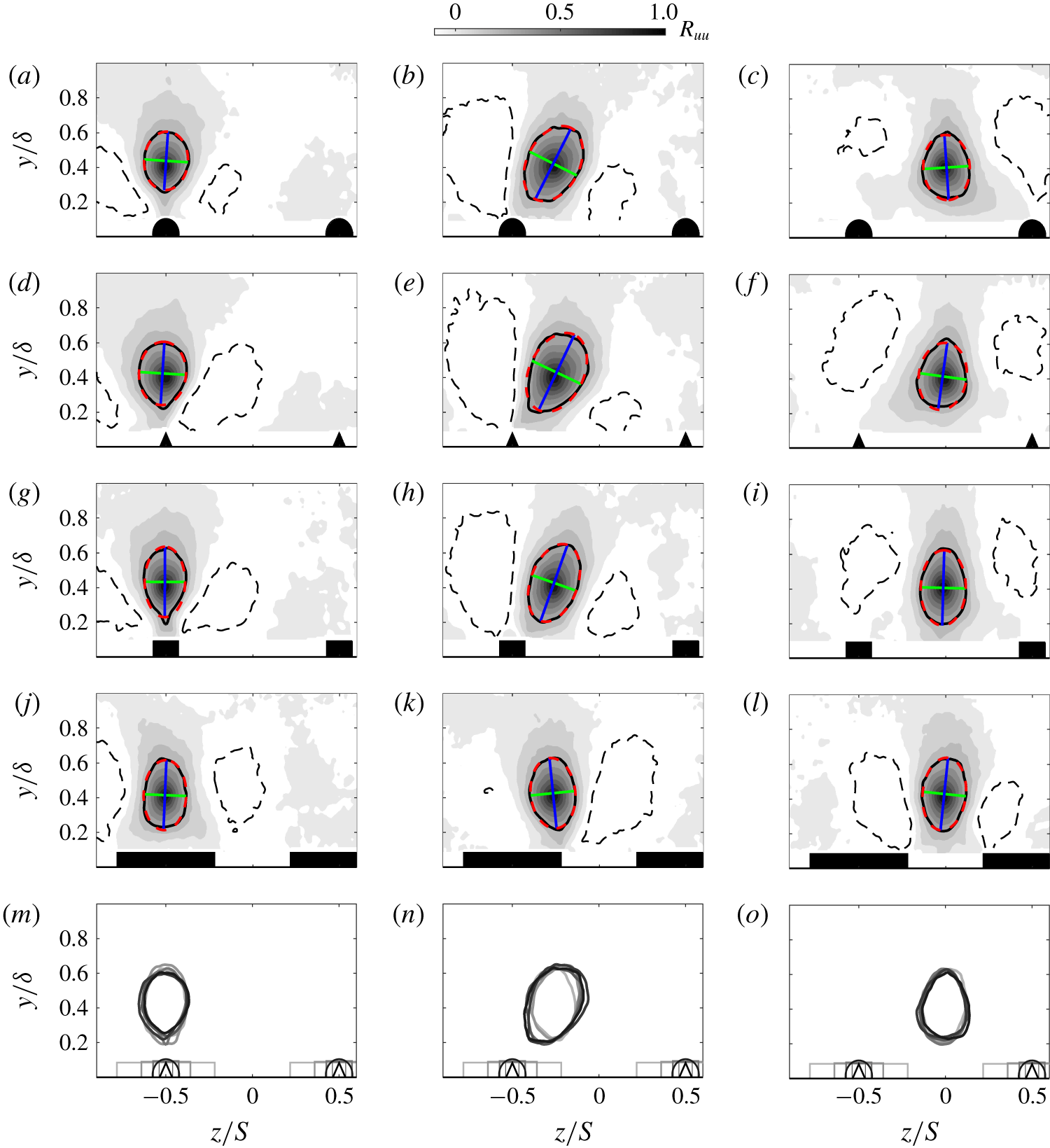
 $(y,z)$ plane. Figure 11 illustrates the two-dimensional autocorrelation maps of the streamwise velocity fluctuation
 $\unicode[STIX]{x1D619}_{uu}$ at
 $y/\unicode[STIX]{x1D6FF}=0.4$ determined at three different spanwise reference locations (
 $z/S=-0.5,-0.25$ and 0 from left to right) for four different heterogeneous surfaces (HS1, HS2, HS4 and HS6). The wall-normal location was chosen to show representative presence or absence of structural similarity in the outer layer while the spanwise locations are chosen to investigate structural changes in the spanwise direction.
Significant changes in the spatial coherence in both the wall-normal and spanwise directions are observed for the different locations. The correlation maps indicate that at the LMPs (figure 11a,d,g,j,m), the structures are skewed in the wall-normal direction, but symmetric in the spanwise direction. They also highlight the emergence of negatively correlated regions shown as the black dashed contour flanking either sides of the ridges. Their spanwise extent appears to extend away from the wall while they shrink when closer to the ridge. In contrast, the structures observed at the HMPs show an opposite behaviour with a much larger spatial coherence near the wall (figure 11c,f,i,l,o) as opposed to a narrower correlation away from the wall. Two negatively correlated regions exist in the spanwise direction with a larger distance away from their main lobe compared to the LMP structure. The asymmetric nature in the horizontal plane of these structures seems to link with the presence of the large-scale secondary motions. In fact, if we pick a point near the wall ( $y=0.2\unicode[STIX]{x1D6FF}$), strong inward radial motions are expected above the ridge, whereas outward radial motions occur at the valley. Likewise, at a location away from the wall (
 $y=0.6\unicode[STIX]{x1D6FF}$), the opposite behaviour is expected to occur. Hence the non-symmetric aspect of the coherent structures observed above the peaks and valleys.
Spatial autocorrelation maps of the fluctuating streamwise velocity  $\unicode[STIX]{x1D619}_{uu}$ in the cross-plane at
 $y_{ref}=0.4\unicode[STIX]{x1D6FF}$ over three spanwise locations: (a,d,g,j,m) peak, (b,e,h,k,n) mid-peak–valley distance and (c,f,i,l,o) valley. (a–c) HS1, (d–f) HS2, (g–h) HS4, (j–l) HS6 and (m–o) a selected contour level of all the cases superimposed. The black contour level represents
 $\unicode[STIX]{x1D619}_{uu}=0.3$. The corresponding ellipsoid fit is represented in red dashed contour with its major and minor axes in blue and green lines, respectively. The dashed black contour level represents
 $\unicode[STIX]{x1D619}_{uu}=-0.1$.

Spanwise variation of (a) the normalised autocorrelation length scale determined at  $\unicode[STIX]{x1D619}_{uu}=0.3$ and (b) the corresponding structure inclination subjected to different surface heterogeneities. Positive and negative angles above and below the blue dashed line refer to clockwise and anticlockwise inclination of the structure. See table 1 for definitions of the symbols.

The correlation maps in the mid-plane between HMPs and LMPs (figure 11b,e,h,k,n) indicate that both their spatial extent as well as their orientations are affected. A significant increase in the coherence of the structures accompanied by a substantial tilt is shown through the black contour level, along with the rise of two non-symmetric negative correlation regions. This inclination is believed to be caused by the strong radial motions induced by the presence of these large-scale secondary flows, which result in the spanwise mean shear flow. In fact, their inclination angles seem to line up reasonably well with the normal to the isolines of the streamwise velocity map (as shown in the figure 4). This is more evident with the observation made for the HS6 case which showed a reversal in the direction of the tilt similar to the swap in the LMP and HMP locations reported for the same surface. Qualitative similarities across cases are observed when comparing the extent of the coherent structure at the peaks and valleys as shown in figure 11(m,o). The exception remains the HS6 case, where the turbulence structure seems to have been altered due to the swap of the LMP and HMP locations.
Quantitative changes in the turbulence structures (coherence inclination angles and length scales) are computed from the  $\unicode[STIX]{x1D619}_{uu}$ map in the
 $(y,z)$ plane. This is done by fitting an ellipsoid to a given contour level (shown with a black solid curve in figure 11 at
 $\unicode[STIX]{x1D619}_{uu}=0.3$). The parameters of this fitted ellipse (red dashed curve) include the two orthogonal axes with a major axis (shown in blue) and a minor axis (shown in green) representing the characteristic length scales in the wall-normal and spanwise directions. An overall length
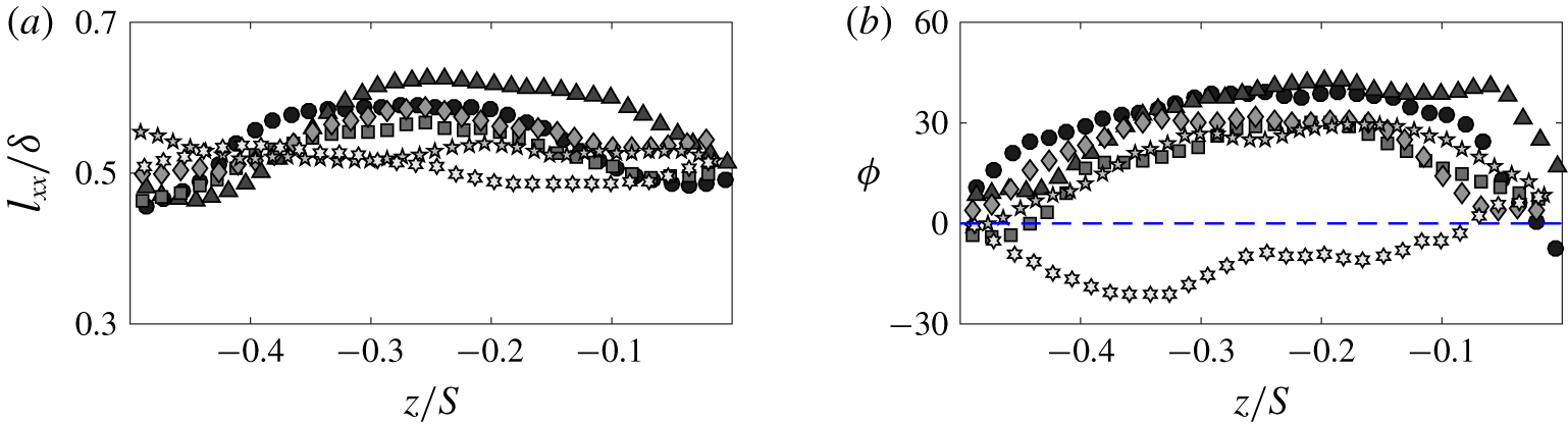
 $l_{xx}$ shown in figure 12(a) is estimated by taking the square root of the sum of the squares of the minor and major axes of the ellipse, while the inclination angle
 $\unicode[STIX]{x1D6F7}$ is just the major axis clockwise rotation from the wall-normal direction as shown in figure 12(b). Both these values seem to have been affected by the surface heterogeneities. The length scale
 $l_{xx}$ seems to grow between the HMP and LMP especially where the spanwise mean shear flow is the highest. This is accompanied by a modification in the turbulence structure shapes which show elongated oblique coherence characterised by their inclination.
These observations are also in agreement with other recent studies of strip-type surfaces from Bai et al. (Reference Bai, Kevin, Hutchins and Monty2018) and Kevin et al. (Reference Kevin, Monty and Hutchins2019). The results from the wall-parallel SPIV performed in the logarithmic region by Bai et al. (Reference Bai, Kevin, Hutchins and Monty2018) revealed that near the surface discontinuity, the coherent structures presented a yawed coherence due to the lateral inflow. This region, which is home to strong wall-normal vortices, induces the high- and low-speed streaks to be arranged above the high roughness (HMPs) and low roughness (LMPs), respectively. This is furthermore supported by the study of Kevin et al. (Reference Kevin, Monty and Hutchins2019) who investigated the characteristics of these coherent structures in multiple streamwise, spanwise as well as wall-parallel planes in the herringbone converging–diverging riblet roughness. They found that between the HMPs and LMPs, the region is home to an appearing ‘detached’ coherent structure which is characterised by a tilt in the wall-normal and streamwise directions that enhances lateral momentum transfer. This is a further evidence that structural similarity has been altered by the secondary flows.
3.6 Effect on the wake intermittency
The turbulent/non-turbulent interface (TNTI) has been widely explored in many flows, such as in wakes, jets and turbulent boundary layers (Bisset, Hunt & Rogers Reference Bisset, Hunt and Rogers2002; Westerweel et al. Reference Westerweel, Fukushima, Pedersen and Hunt2005; Laskari et al. Reference Laskari, de Kat, Hearst and Ganapathisubramani2018). The TNTI represents an instantaneous thin layer that isolates regions of turbulent motions from regions of non-turbulent flow (Corrsin & Kistler Reference Corrsin and Kistler1955). The interface is characterised by a simultaneous occurrence of small- and large-scale processes termed ‘nibbling’ and ‘engulfment’, representative of viscous and inertial mechanisms, inducing turbulence-free fluid entrainment towards the turbulent flow (Chauhan et al. Reference Chauhan, Philip, de Silva, Hutchins and Marusic2014). In the presence of surface spanwise heterogeneity, both the inner and outer regions were shown to be affected by the large-scale secondary motions, which rearrange the structural organisation of the turbulence (Kevin et al. Reference Kevin, Monty, Bai, Pathikonda, Nugroho, Barros, Christensen and Hutchins2017; Yang & Anderson Reference Yang and Anderson2017; Bai et al. Reference Bai, Kevin, Hutchins and Monty2018; Kevin et al. Reference Kevin, Monty and Hutchins2019). Therefore, this raises the question as to how the wake intermittency re-adapts to the structural changes observed before.
Effect of different threshold levels on the tortuosity parameter for the different heterogeneous surfaces. The vertical red dashed line represents the selected threshold  $\tilde{k}_{th}/\tilde{k}_{\infty }=4$ for the TNTI analysis. See table 1 for definitions of the symbols.

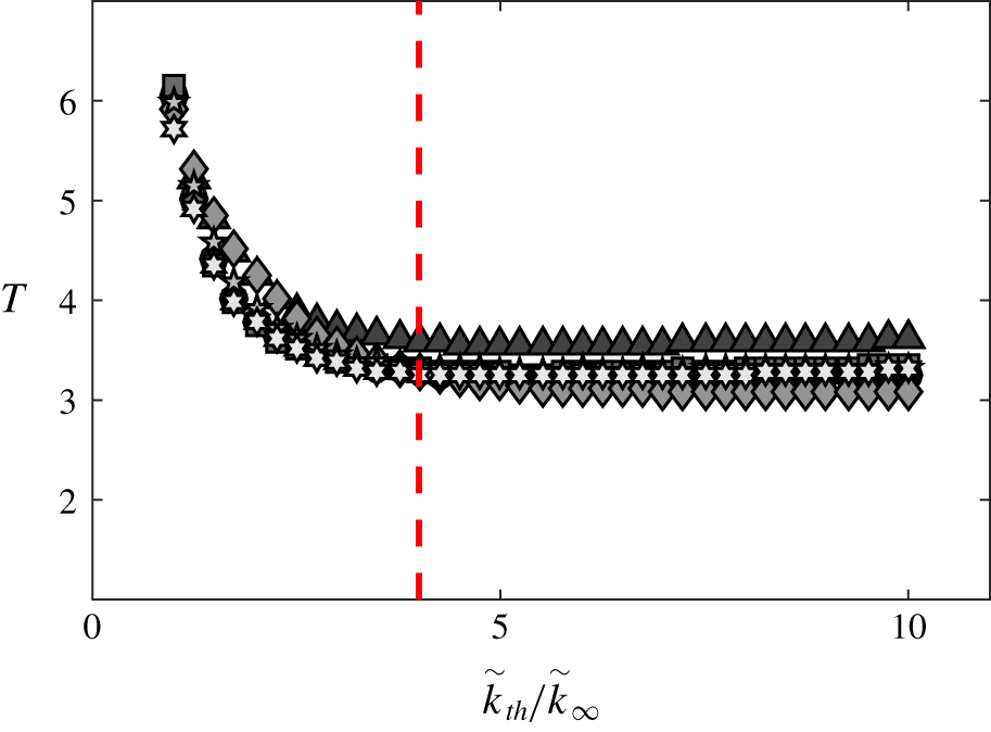
The interface detection method currently employed is similar to that defined by Chauhan et al. (Reference Chauhan, Philip, de Silva, Hutchins and Marusic2014), based on a local turbulent kinetic energy deficit detector  $\tilde{k}_{th}$, of a given threshold that separates the instantaneous flow into a turbulent and non-turbulent flow. However, the threshold selection is shown to be specific to each experiment and can be influenced by the turbulence level in the free stream, the measurement systematic and statistical uncertainties. Consequently, in order to have a consistent way of defining suitable thresholds for the different cases, a variable
 $T$ defined as the ‘tortuosity’ is determined for different levels of thresholds. The tortuosity essentially represents the arc length of the interface
 $l_{i}$ within a given unit distance, herein defined as
 $T=l_{i}/S$. Figure 13 illustrates the variation of the tortuosity as a function of the threshold level
 $\tilde{k}_{th}$ normalised by the turbulent kinetic energy deficit in the free stream
 $\tilde{k}_{\infty }$. The results indicate that beyond a certain level, the tortuosity becomes constant irrespective of changes in the threshold level
 $\tilde{k}_{th}/\tilde{k}_{\infty }$. The value
 $\tilde{k}_{th}/\tilde{k}_{\infty }=4$ was found to correspond to a reasonable threshold level that yields a consistent comparison between cases. In this case,
 $4\tilde{k}_{\infty }$ ranges between 0.12 and 0.25, which are between a factor one and two of the value used by Chauhan et al. (Reference Chauhan, Philip, de Silva, Hutchins and Marusic2014). However, as mentioned above, these values are not expected to remain constant from one experiment to another.
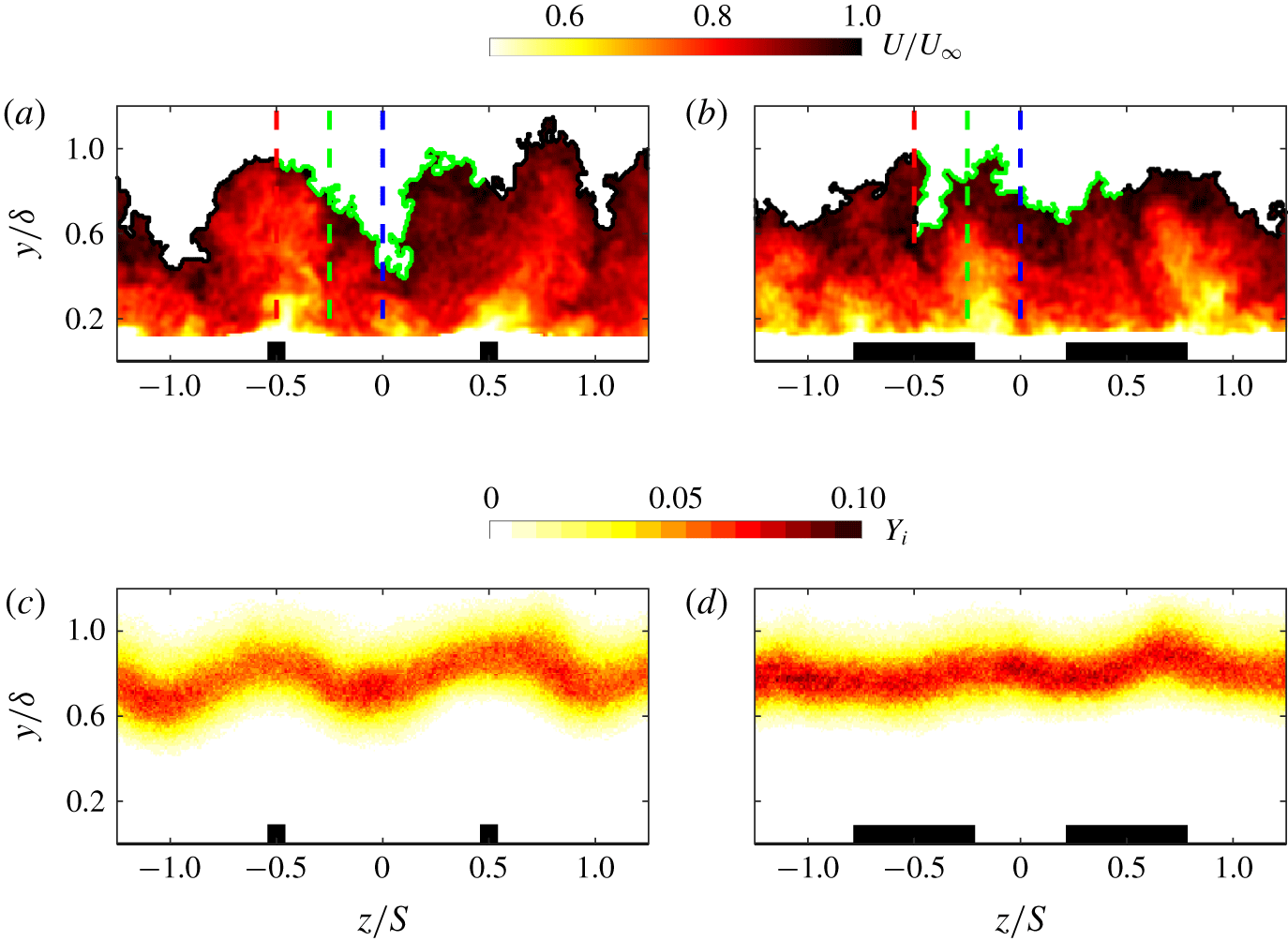
To demonstrate the effect of the surface heterogeneity on the interface, two examples for HS3 and HS6 are highlighted in figures 14(a) and 14(b), respectively. The TNTI is shown in figure 14(a,b) as the black contour delineating two distinct regions in the instantaneous streamwise velocity map: turbulence-free stream above and turbulent regions below the interface outline. The arc length of the TNTI within a spanwise unit distance used to determine the tortuosity is highlighted in green. Figure 14(a) clearly indicates that substantial distortions are present at the interface outline, with alternating large-scale bulges and valleys above the elevated and recessed surfaces, respectively. This observation remains consistent for all cases except HS6 as shown in figure 14(b), which showed the occurrence of the opposite behaviour.
Example of the application of the turbulent kinetic energy deficit criterion to an instantaneous streamwise velocity map for (a) HS3 and (b) HS6. The TNTI outline is highlighted with a black line. The arc length used to determined the tortuosity in figure 13 is shown inside one wavelength in green. The colour-coded vertical dashed lines are the spanwise locations over which the local intermittency profiles are evaluated as shown in figure 15(a,b). The ensemble averages of the spatial occurrence on the TNTI in the  $(y,z)$ plane for (c) HS3 and (d) HS6.

In order to get a quantitative assessment of these differences, the TNTIs of all the snapshots are superimposed to obtain an ensemble average as illustrated in figure 14(c,d). As expected, the wall-normal location of the TNTI appears to undergo a similar periodicity to the mean flow in the spanwise direction, with alternating high and low TNTI locations above the elevated and recessed surface, respectively. Furthermore, the changes observed in the mean and the turbulent characteristics for HS6 are also reflected in figure 14(d), which is characterised by a swapping of the high and low TNTI locations. The spanwise variation of the interface seems to also have a subtle dependence on the strength of secondary flows. In fact, the maps of the TNTI height  $Y_{i}$ indicate that the peak-to-peak for HS3 is higher than that for HS6. However, this is not completely clear when the tortuosity of the interface is examined as shown in figure 13. It appears that the most tortuous interface is HS2, which was shown to be the most heterogeneous flow. Nevertheless, the rest of the cases seem to have relatively similar values of
 $T$ which range between 3.2 and 3.6 for the different cases.
It is perhaps also interesting to point out that the values of  $T$ are in reasonable agreement with the predicted value of Chauhan et al. (Reference Chauhan, Philip, de Silva, Hutchins and Marusic2014) for a smooth-wall turbulent boundary layer. They hypothesised that based on the fractal nature of the TNTI, its length in the spanwise direction is expected to be three times the distance on where it sits, similar to that in the streamwise direction. In the present study, the induced cross-plane secondary motions caused by the surface heterogeneity have effectively altered the interface, hence the slightly larger values of the tortuosity. Similar findings have also been recently reported by Kevin et al. (Reference Kevin, Monty, Bai, Pathikonda, Nugroho, Barros, Christensen and Hutchins2017), who observed strong spanwise waviness of the TNTI. Their analysis was based on the identification of ‘pockets’ of turbulence-free fluid within the turbulent flow below the interface outline. After looking at both the spatial distribution of these non-turbulent pockets as well as their frequency of occurrence, they observed that their manifestation is two times more probable over the downwash than the upwash regions. They showed that this was due to large-scale free-stream engulfment occurring close to the wall, in contrast to less recurrent pockets over the upwash regions which appeared far from the wall.
Wall-normal distribution of the local intermittency profiles  $\unicode[STIX]{x1D6FE}$ for (a) HS3 and (b) HS6 at
 $z/S=-0.5,-0.25$ and
 $0$ for the red, green and blue markers, respectively. (c) The corresponding probability density function
 ${\mathcal{P}}(y_{i})$ for HS3 with the inset comparing the profile at
 $z/S=-0.5$ (red squares) to a Gaussian distribution (dashed line) normalised with the variance. (d) The global probability density function of the TNTI
 ${\mathcal{P}}(Y_{i})$ locations for the different cases. The left-hand and right-hand insets of (d) highlight the profile of HS3 (solid line) compared with a Gaussian distribution (dashed line) normalised by the variance, and the profiles of all the cases colour-coded as shown by the symbol definitions in table 1.

The intermittency  $\unicode[STIX]{x1D6FE}$ indicates the proportion of time a flow is turbulent at a given point in the
 $(y,z)$ plane. Consequently,
 $\unicode[STIX]{x1D6FE}$ tends to 1 near the wall whereas it tends to 0 near the free stream. The local intermittency profiles are shown for three different spanwise locations for HS3 and HS6 in figures 15(a) and 15(b), respectively. The different colours highlight the three spanwise locations illustrated with vertical coloured dashed lines in figure 14(a,b). The profiles indicate the intermittency to have a constant upper bound beyond which the flow remains statistically laminar, when the wall-normal distance is scaled with the local boundary layer thickness. On the other hand, the insets of figure 15(a,b) reveal that the lower bound changes according to the spanwise location. For example, figure 15(a) indicates that the intermittency extent is wider at the valley (
 $z/S=0$ and
 $-0.25$) than over the ridge (
 $z/S=-0.5$) which correspond to the downwash and upwash regions, respectively. This result is in fact not surprising since the ridges give rise to high-turbulence fluxes, which are then advected vertically, causing the reduction in the wake intermittent activity at the ridge. Conversely, the recessed regions are dominated by downwash motions transporting low-turbulence fluxes towards the near wall rendering the intermittent region larger. As expected, these results are shown to be valid for all the cases with the exception of HS6. This is demonstrated in figure 15(b) which highlights the occurrence of an opposite behaviour, where the profiles above the ridge appear to have an extended intermittent region, although the differences being weaker. These changes between HS6 and HS3 (as well as the rest of the cases) are expected to take place since we previously observed the HMPs and LMPs to have swapped locations. This wake behaviour means that the HMPs (downwash) will always induce larger intermittency extents, while the LMPs (upwash) will generate shorter intermittency extents.
Finally, the probability density function of the local TNTIs,  ${\mathcal{P}}(y_{i})$, is examined in figure 15(c) for HS3. The profiles reveal that the local mean heights of the TNTI
 $\overline{y_{i}}$ vary marginally in the spanwise direction. This is also highlighted by the vertical and horizontal black dashed lines which correspond to
 $\unicode[STIX]{x1D6FE}=0.5$ in figure 15(a,b). The structural modifications in the outer region also appear to have affected the Gaussian nature of the TNTIs, specifically at the LMP. This is illustrated in the inset of figure 15(c) which compares the local profile at the upwash region (red squares) against a Gaussian distribution (black dashed line), which shows a degree of skewness towards the free stream. This observation, however, is only true in the local sense. Globally, the profiles are shown to remain Gaussian regardless of the surface heterogeneity. This is depicted in figure 15(d) which inspects the global probability density function
 ${\mathcal{P}}(Y_{i})$ across cases. Despite the differences in the mean TNTI height
 $\overline{Y_{i}}$ which is in the range
 $0.77\leqslant \overline{Y_{i}}/\unicode[STIX]{x1D6FF}\leqslant 0.86$, the distributions appear to have a good degree of symmetry. As a matter of fact,
 ${\mathcal{P}}(Y_{i})$ for HS3 is presented in the left-hand inset of figure 15(d), and shows an excellent degree of collapse with the Gaussian distribution (black dashed line). This indicates that, in spite of the presence of large-scale secondary flows, the Gaussian nature of the TNTI globally remains unaffected. The secondary flows are shown to mainly induce changes in the extent of the intermittent regions. The right-hand inset of figure 15(d) displays that the TNTI extent becomes larger for cases that exhibit stronger secondary motions. This is shown by the changes in the standard deviation of the interface which is in the range
 $0.11\leqslant \unicode[STIX]{x1D70E}_{Y_{i}}/\unicode[STIX]{x1D6FF}\leqslant 0.19$ from the least to most heterogeneous case.
Overall, the results highlighted from the TNTI analysis are consistent with the recently observed changes in the wake strength parameter  $\unicode[STIX]{x1D6F1}$ reported by Medjnoun et al. (Reference Medjnoun, Vanderwel and Ganapathisubramani2018). In fact, by measuring directly the local friction velocity and the corresponding velocity profile across different spanwise locations, they showed the wake strength parameter to be affected by the surface spanwise heterogeneity (hence the flow heterogeneity). They found that the elevated and recessed regions of the surface (corresponding to the LMPs and HMPs, respectively) resulted in low and high values of
 $\unicode[STIX]{x1D6F1}$, respectively. As indicated by Krug, Philip & Marusic (Reference Krug, Philip and Marusic2017), the wake strength parameter stems from a dual effect of the velocity jump across the TNTI as well as the uniform momentum zones. Therefore, the previously observed changes in the wake parameter are probably due to the changes in the intermittent activity across the span. While the current results highlight the effect of the large-scale secondary motions on the wake intermittency, further studies remain necessary to also examine their impact on the uniform momentum zones.
4 Discussion
Two questions that have drawn the attention of researchers are the prediction of the HMPs and LMPs for various wall conditions and the identification of important surface features that can scale the secondary flows. Based on existing literature, we found two main categories of surfaces that seemingly exhibit similar flow attributes, yet have different triggering mechanisms of secondary flows.
Sketch illustrating the effect of the ridge/roughness width for (a) ridge-type and (b) strip-type heterogeneities. The secondary motions and mean flow curvature are highlighted as clockwise/anticlockwise red/blue circles and black dashed lines.

For the skin-friction-based heterogeneity whose surface alternates between high and low wall shear stress (due to surface roughness or superhydrophobic surfaces etc.), both the width of the high/low skin friction and the characteristic spanwise wavelength were shown to be relevant. Willingham et al. (Reference Willingham, Anderson, Christensen and Barros2014) showed that by keeping the spanwise wavelength constant, increasing the high drag width produced stronger mean flow heterogeneity. They showed that the HMPs and LMPs systematically occurred above the high and low wall shear stress, respectively. On the other hand, Stroh et al. (Reference Stroh, Hasegawa, Kriegseis and Frohnapfel2016) varied both the spanwise wavelength and the low shear-stress width and reported their important influence on the flow topology. They showed that for a relatively thin strip of high shear stress, HMPs and LMPs occurred above the low and high wall shear stress, respectively. For increased strip widths, the opposite behaviour occurred. Chung et al. (Reference Chung, Monty and Hutchins2018) have also showed by keeping the high to low roughness widths constant and just increasing the spanwise wavelength, the HMPs and LMPs are always observed above the high and low wall shear stress, respectively. The exception being that for very large wavelengths (both large high/low skin-friction widths), the HMPs and LMPs appeared above the low and high skin friction, respectively. This is confirmation that local homogeneity of the flow can be recovered (away from the discontinuity), with high and low roughness producing thicker and thinner boundary layer thickness. Hence, the different studies indicate that perhaps more than one length scale should be considered for characterising the surface heterogeneity.
Most of the previous studies of the ridge-type heterogeneous surfaces showed that the spanwise wavelength is relevant for the presence of the secondary flows (Nezu & Nakagawa Reference Nezu and Nakagawa1984; Vanderwel & Ganapathisubramani Reference Vanderwel and Ganapathisubramani2015; Yang & Anderson Reference Yang and Anderson2017; Hwang & Lee Reference Hwang and Lee2018). Analogous to the study of Willingham et al. (Reference Willingham, Anderson, Christensen and Barros2014), the current results highlighted the importance of an additional surface feature depicted by the ratio of the recessed and elevated regions in addition to the spanwise wavelength. This analogy between the two wall conditions is sketched in figures 16(a) and 16(b) for the ridge- and roughness-type heterogeneities, respectively, for a fixed wavelength  $S$. By drawing on the results from the current and previous studies, we can identify notable differences in the two types. Considering a generic shape such as a rectangle of a given height and varying widths to represent the ridge-type heterogeneity, we can observe manifestations of secondary motions in the form of large-scale streamwise rollers flanking the ridges, and perhaps tertiary structures as shown in this and many other studies. For very thin ridges, strong secondary motions are expected (similar to HS2) with upwash and downwash occurring above and between the ridges. Increasing the width results in the appearance of the tertiary structures competing with the large secondary structures above the ridge, thereby weakening the mean flow heterogeneity. Increasing the width beyond a certain limit results in the swap of HMPs and LMPs, albeit with a lower level of the flow heterogeneity, until the flow reaches homogeneity again. In the case of roughness-type heterogeneity, the secondary flows are expected to remain confined in the vicinity of the stress discontinuity for the limits of very wide/narrow strips. This results in a weak Reynolds shear-stress heterogeneity causing the base flow to remain homogeneous. Between these two limits, the secondary flows reach their full potential over a range of widths, then will decrease eventually when increasing/decreasing above/below a certain limit.
In view of these results, it is clear that the spanwise wavelength is not sufficient on its own to describe the flow heterogeneity. A surface heterogeneity parameter  ${\mathcal{H}}$ can be considered as a combination of
 $S$ and an additional surface parameter
 $\unicode[STIX]{x1D709}$:
 $$\begin{eqnarray}{\mathcal{H}}=F\left(\frac{S}{\unicode[STIX]{x1D6FF}},\unicode[STIX]{x1D709}\right).\end{eqnarray}$$
In the case of a ridge-type heterogeneity, we have shown in this study that  $\unicode[STIX]{x1D709}$ can be expressed as a ratio of the area/perimeter of the elevated and recessed regions. This was shown to capture both the shape and width variations of the ridges. In the case of a roughness-type heterogeneity,
 $\unicode[STIX]{x1D709}$ can be related to a ratio of the high to low roughness (or high to low shear stress) weighted by the respective widths. Overall, the spanwise heterogeneity can be thought of as a combination of at least two parameters: first, a spanwise characteristic wavelength (
 $S/\unicode[STIX]{x1D6FF}$), which represents an onset condition necessary to trigger large-scale spanwise fluctuations; second, a geometrical parameter (represented herein as the ratio of the recessed and elevated areas (
 $\unicode[STIX]{x1D709}$) necessary to amplify or reduce these radial motions. Therefore, one can influence the secondary motions by varying
 $S/\unicode[STIX]{x1D6FF}$ while keeping
 $\unicode[STIX]{x1D709}$ constant (see e.g. Chan et al. (Reference Chan, MacDonald, Chung, Hutchins and Ooi2018)), alternatively by keeping
 $S/\unicode[STIX]{x1D6FF}$ constant and changing
 $\unicode[STIX]{x1D709}$ (such as in the present investigation). For the ridge-type surfaces considered here, the relationship between the secondary flow circulation and
 $\unicode[STIX]{x1D709}$ appears to be linear for a fixed
 $S/\unicode[STIX]{x1D6FF}$ over the range of
 $\unicode[STIX]{x1D709}$ examined here.
The second question that has garnered attention is the spanwise locations of the HMPs and LMPs for the ridge-type heterogeneity. Several studies reported similar findings to ours when  $S/\unicode[STIX]{x1D6FF}\approx O(1)$ (Nezu & Nakagawa Reference Nezu and Nakagawa1984; Colombini Reference Colombini1993; Wang & Cheng Reference Wang and Cheng2006; Vanderwel & Ganapathisubramani Reference Vanderwel and Ganapathisubramani2015; Hwang & Lee Reference Hwang and Lee2018; Vanderwel et al. Reference Vanderwel, Stroh, Kriegseis, Frohnapfel and Ganapathisubramani2019). Contrastingly, other recent investigations showed that the opposite scenario can occur (Mejia-Alvarez & Christensen Reference Mejia-Alvarez and Christensen2013; Barros & Christensen Reference Barros and Christensen2014; Yang & Anderson Reference Yang and Anderson2017; Awasthi & Anderson Reference Awasthi and Anderson2018). However, one of the key differences between these two sets of studies is the presence/absence of streamwise homogeneity of the surface. In fact, all the studies that reported the upwash above the surface elevations used streamwise continuous ridges, in contrast with the studies that reported downwash to occur above the elevated regions. The highly irregular roughness of Mejia-Alvarez & Christensen (Reference Mejia-Alvarez and Christensen2013) and Barros & Christensen (Reference Barros and Christensen2014) and the highly ordered roughness of Yang & Anderson (Reference Yang and Anderson2017) and Awasthi & Anderson (Reference Awasthi and Anderson2018) clearly exhibit wake-producing protrusions, which induce form-drag contributions. Therefore, despite these surfaces being topographically heterogeneous, they appear to act more like high/low wall-shear-stress-producing surfaces, in contrast with the previous ones which are predominantly viscous-drag-producing surfaces. The exception was the surface studied by Vanderwel & Ganapathisubramani (Reference Vanderwel and Ganapathisubramani2015) which also contained form-drag-producing pins. However these protrusions were homogeneously distributed over the surface, meaning that their overall contributions remained uniform as opposed to Yang & Anderson (Reference Yang and Anderson2017) and Awasthi & Anderson (Reference Awasthi and Anderson2018) which were localised only at the surface elevations. Although this explanation may seem plausible following the rule of ‘high’ and ‘low’ roughness generating downwash and upwash, respectively, this is clearly not the case for the staggered sinusoidal roughness investigated by Chan et al. (Reference Chan, MacDonald, Chung, Hutchins and Ooi2018). In fact, they reported the HMPs and LMPs to be located between the peaks and valleys of the topography, corresponding to regions of low and high wall shear stress. Consequently, the differences between the driving mechanisms behind the direction of the secondary flows for staggered and non-staggered roughness need further exploration.
Finally, the utility of outer-layer similarity in flows with secondary motions has been questioned and examined. Based on the experimental work of Wu & Christensen (Reference Wu and Christensen2007, Reference Wu and Christensen2010) and Pathikonda & Christensen (Reference Pathikonda and Christensen2017), both mean flow and structural similarity were shown to exist despite the emergence of secondary flows. This is in contrast to other investigations that showed outer-layer similarity to be affected in first- and second-order moments as well as spectra (Yang & Anderson Reference Yang and Anderson2017; Chung et al. Reference Chung, Monty and Hutchins2018; Medjnoun et al. Reference Medjnoun, Vanderwel and Ganapathisubramani2018). Chan et al. (Reference Chan, MacDonald, Chung, Hutchins and Ooi2018) provided useful insight onto the conditions of validity of the similarity hypothesis, based on the quantification of the dispersive stresses. They showed that as long as these form-induced stresses remained only prominent near the canopy layer, the turbulent structures in the outer region remain unaffected by the secondary flows. However, this only occurs for very small spanwise wavelengths. As soon as the wavelength is comparable to the dominant length scale of the flow, the secondary motions occupy a large portion of the flow, which induce dispersive stresses that extend farther in the outer region. Our current findings also corroborate these observations such that the cases presenting strong secondary motions showed lack of outer-layer similarity. It is also important to recall that the primary condition for outer-layer similarity is a substantial separation between large- and small-scale separation (Jiménez Reference Jiménez2004; Castro Reference Castro2007; Flack & Schultz Reference Flack and Schultz2014; Squire et al. Reference Squire, Morrill-Winter, Hutchins, Schultz, Klewicki and Marusic2016). In the case of the study by Barros & Christensen (Reference Barros and Christensen2014), their surface roughness exhibited a wide range of multiscale features as opposed to the other studies. These roughness features are likely to enhance near-wall mixing and increase the overall drag and the scale separation. This combined with perhaps relatively mild dispersive stresses can result in the validity of outer-layer similarity.
5 Conclusions
A turbulent boundary layer flow over smooth heterogeneous surfaces has been experimentally studied. We specifically looked at the influence of different surface heterogeneities on the secondary flows that developed under these conditions. Oil-film interferometry along with SPIV measurements allowed us to evaluate the impact of these heterogeneous surfaces on the skin friction and the mean and turbulent flow properties.
In the presence of a ridge-type surface heterogeneity, the spanwise distribution of the skin friction varies as a consequence of the mean flow heterogeneity. As a result, strong spanwise skin-friction gradients are observed, and are located near regions of high spanwise mean shear. The average frictional drag was directly assessed and was shown to be a function of both Reynolds number as well as the surface heterogeneity. It is speculated that these surfaces do not allow the flow to transition to a ‘fully’ rough regime, as the roughness function is entirely driven by the viscous drag and has no form drag due to lack of streamwise roughness protrusion.
The mean vertical velocity component emphasised the importance of both the ridge shape and width. It is shown that beyond a given value of width, a swap between the HMPs and LMPs can occur. For  $(S-W)/\unicode[STIX]{x1D6FF}>0.5$, the HMPs and LMPs were consistently shown to occur above the recessed and elevated regions of the surface. The modifications were also evident in the streamwise vorticity highlighted by the swirling strength, revealing marked changes in the secondary flow structures. Strong secondary motions occurred above thin ridges when
 $(S-W)/\unicode[STIX]{x1D6FF}\approx O(1)$, whose extent is shown to scale with the valley width, while their strength scales with the ridge curvature. For rectangular ridges, a pair of new small counter-rotating vortices of opposed sign emerge above the ridges forming tertiary structures. For
 $(S-W)/\unicode[STIX]{x1D6FF}\leqslant 0.5$, an imbalance in favour of the tertiary vortices occurs which take over the secondary ones, leading to the swap of the LMP and HMP locations. The results also indicated that the spanwise spacing alone is insufficient to characterise the surface heterogeneity. An additional parameter based on the ratio of perimeters of recessed and elevated regions,
 $\unicode[STIX]{x1D709}$, was adopted. It adequately captured the changes in shapes and widths of the ridges highlighting the effects of the heterogeneity on drag and the streamwise circulation in the outer layer.
Triple decomposition of the velocity components allowed the examination of the surface heterogeneity through the dispersive stresses. We determined qualitatively and quantitatively the contributions of the form-induced stresses to the total shear stress, which varied from  $15\,\%$ to
 $55\,\%$, proportional to the strength of the secondary motions. The total shear-stress estimates were subsequently used to examine outer-layer similarity in the mean and turbulence statistics. The results indicated lack of similarity in the mean flow; however, a collapse with the smooth wall is observed in the diagnostic form. This observation indicates that the secondary motions affect proportionally the mean flow and the turbulent structure in the outer region.
The two-point correlation maps of the streamwise velocity fluctuations  $\unicode[STIX]{x1D619}_{uu}$ allowed the examination of the turbulence structures in the outer region. The structures exhibit spanwise symmetry above the LMPs and HMPs, while they are asymmetric in the wall-normal direction due to the intense inward/outward radial motions. In the mid-distance between the LMPs and HMPs, the turbulent structures exhibited a higher coherence accompanied by a substantial inclination towards the HMPs, which is consistent with previous studies. The analysis of the TNTI revealed the impact of the secondary flows on the wake intermittency. Instantaneous snapshots showed the existence of strong bulges and valleys in the interface outline, which is translated in TNTI undergoing a spanwise modulation. The extent of the intermittency is shown to vary across the spanwise direction with shorter and larger intermittency extents at the upwash and downwash regions, respectively. The global probability density function of the TNTI indicated that the main impact of the secondary flows is the change in the intermittency extent, with stronger secondary flows inducing a larger extent.
Acknowledgements
The authors acknowledge financial support of the Engineering and Physical Sciences Research Council of the United Kingdom (EPSRC grant nos EP/L006383/1 and EP/P021476/1). C.V. is supported by a Marie Curie fellowship (project no. 656081). T.M. is also partially supported by the Faculty of Engineering and Physical Sciences at the University of Southampton. The authors would like to also acknowledge the insightful comments and pertinent observations of the referees during the review process of the manuscript. All data supporting this study are openly available from the University of Southampton repository at https://doi.org/10.5258/SOTON/D1155.
Declaration of interests
The authors report no conflict of interest.