2. Near-axis expansion

In this section, we introduce the near-axis expansion using the direct coordinate approach first derived by Mercier (Reference Mercier1964). We denote the magnetic axis as the curve $\boldsymbol {r}_0(s)$ having total length $L$, with $s$ as the arclength. The tangent $\boldsymbol {t}(s) = \boldsymbol {r}_0'(s)$, the normal $\boldsymbol {n}(s) = \boldsymbol {t}'(s)/\kappa$ and the binormal $\boldsymbol {b}(s) = \boldsymbol {t} \times \boldsymbol {n}$ unit vectors form the orthogonal Frenet–Serret frame (Spivak Reference Spivak1999), which satisfy the first-order Frenet–Serret equations $\boldsymbol {t'}(s) = \kappa \boldsymbol {n}$, $\boldsymbol {n'}(s) = -\kappa \boldsymbol {t} + \tau \boldsymbol {b}$ and $\boldsymbol {b'}(s) = -\tau \boldsymbol {n}$. The curvature $\kappa$ and the torsion $\tau$ are found using

(2.1)\begin{equation} \kappa(t) = \frac{\lvert \boldsymbol{r}_0'(t) \times \boldsymbol{r}_0''(t)\rvert}{\lvert \boldsymbol{r}_0'(t)\rvert^2}, \end{equation}

and

(2.2)\begin{equation} \tau(t) = \frac{[\boldsymbol{r}_0'(t) \times \boldsymbol{r}_0''(t)] \boldsymbol{\cdot} \boldsymbol{r}_0'''(t)}{\lvert \boldsymbol{r}_0'(t) \times \boldsymbol{r}_0''(t)\rvert^2}, \end{equation}

with $t$ as any quantity that parameterizes $\boldsymbol {r}_0$. Finally, we note that the triad $(\boldsymbol {t},\boldsymbol {n},\boldsymbol {b})$ is uniquely determined by the Frenet–Serret equations above.

To describe a point outside the magnetic axis, we consider a plane between an arbitrary point $\boldsymbol {r}$ and a point on the magnetic axis $\boldsymbol {r}_0$ such that the axis is normal to that plane. The position vector $\boldsymbol {r}$ can then be written as

(2.3)\begin{equation} \boldsymbol{r} = \boldsymbol{r}_0(s) + \rho\cos\theta\boldsymbol{n}(s) + \rho\sin\theta\boldsymbol{b}(s), \end{equation}

with $\rho$ as the distance between $\boldsymbol {r}$ and $\boldsymbol {r}_0$, and $\theta$ is the angle between the normal and $\boldsymbol {r}-\boldsymbol {r}_0$. Alternatively, this plane can be visualized as a Cartesian plane mapped onto the $(\boldsymbol {n},\boldsymbol {b})$ plane with $x = \rho \cos \theta$ and $y = \rho \sin \theta$. We now introduce the angle $\omega = \theta + \gamma (s)$, where $\gamma$ is the integrated torsion $\gamma (s) = \int _0^s \tau (s') \,\textrm {d}s'$, which renders the coordinates $(\rho ,w,s)$ orthogonal. The Jacobian in $(\rho ,\omega ,s)$ coordinates is then given by $\sqrt {g} = \rho h_s = \rho (1-\kappa \rho \cos ({\omega - \gamma (s)})$.

We decompose the magnetic field as $\boldsymbol {B} = B_\rho \boldsymbol {e}_\rho + B_\omega \boldsymbol {e}_\omega + B_s\boldsymbol {e}_s$, with $\boldsymbol {e}_\rho = \cos \theta \boldsymbol {n} + \sin \theta \boldsymbol {b}$, $\boldsymbol {e}_\omega = -\sin \theta \boldsymbol {n} + \cos \theta \boldsymbol {b}$, and $\boldsymbol {e}_s = \boldsymbol {t}$, and similarly for the current density $\boldsymbol {J} = \boldsymbol {\nabla } \times \boldsymbol {B}$. Each scalar function is then expanded in a power series in terms of $\epsilon \rho$, i.e.

(2.4)\begin{equation} B_\rho = \sum_{n=0}^{\infty} B_{\rho n}(\omega,s)\epsilon^n \rho^n. \end{equation}

We note that in a vacuum, as the current density vanishes, $\boldsymbol {B}$ is a curl-free field, i.e. $\boldsymbol {\nabla } \times \boldsymbol {B} = 0$. In this case, a scalar potential function $\phi$ with $\boldsymbol {B} = \boldsymbol {\nabla }\phi$ satisfying Laplace's equation can be used. In orthogonal Mercier's coordinates $(\rho , \omega , s)$, Laplace's equation can be written as

(2.5)\begin{equation} \nabla^2\phi = \frac{1}{\epsilon^2\rho}\frac{\partial}{\partial\rho}\left(h_s\rho\frac{\partial \phi}{\partial\rho}\right) + \frac{1}{\epsilon^2\rho^2}\frac{\partial}{\partial\omega}\left(h_s\frac{\partial\phi}{\partial\omega}\right) + \frac{\partial}{\partial s}\left(\frac{1}{h_s}\frac{\partial\phi}{\partial s}\right) = 0. \end{equation}

A more detailed treatment of (2.5) can be found in the paper by Jorge et al. (Reference Jorge, Sengupta and Landreman2020b).

To simplify the derivation and reduce the number of scalar functions to compute, we write the magnetic field using a Clebsch representation (Helander Reference Helander2014)

(2.6)\begin{equation} \boldsymbol{B} = \boldsymbol{\nabla}\psi \times \boldsymbol{\nabla}\alpha, \end{equation}

where $\alpha$ is a field line label and $\psi$ is the magnetic toroidal flux

(2.7)\begin{equation} \psi = \frac{1}{L}\int(\boldsymbol{B} \boldsymbol{\cdot} \boldsymbol{\nabla} s)\,\textrm{d}V. \end{equation}

Both $\psi$ and $\alpha$ are expanded in powers of $\epsilon \rho$ similarly to (2.4). An equation for the toroidal flux $\psi$ can be found by writing the constraint $\boldsymbol {B} \boldsymbol {\cdot } \boldsymbol {\nabla } \psi = 0$ in Mercier's coordinates, which yields

(2.8)\begin{equation} B_\rho\frac{\partial\psi}{\partial\rho} + B_\omega\frac{1}{\rho^2}\frac{\partial\psi}{\partial\omega} + B_s\frac{\epsilon}{h_s}\frac{\partial\psi}{\partial s} = 0. \end{equation}

Assuming that $\psi$ is analytic close to the magnetic axis (see Kuo-Petravic & Boozer (Reference Kuo-Petravic and Boozer1987) and Jorge et al. (Reference Jorge, Sengupta and Landreman2020b) equations (2.12)–(2.14) for more details on the Fourier series expansion of analytic functions near the axis in the Frenet–Serret frame), we write each component of $\psi$ as

(2.9)\begin{equation} \psi_n(\omega,s) = \sum_{p=0}^{n} \psi_{np}^{c}(\omega,s)\cos p\theta + \psi_{np}^{s}(\omega,s)\sin p\theta, \end{equation}

where the angle $\theta =\omega -\gamma (s)$ is used as all physical quantities must be periodic in $\theta$ (but not necessarily in $\omega$). Noting that $\psi = O(\rho ^2)$ from the constraint in (2.7), we write its lowest order components as

(2.10)\begin{equation} \psi_2 = \frac{B_0{\rm \pi}}{\sqrt{1-\mu^2}}(1 + \mu\cos 2u), \end{equation}

and

(2.11)\begin{equation} \psi_3(\omega,s) = \psi_{31}^{c}\cos u + \psi_{31}^{s}\sin u + \psi_{33}^{c}\cos 3u + \psi_{33}^{s}\sin 3u, \end{equation}

where $B_0$ is the on-axis magnetic field, $u = \theta + \delta (s)$, and $\delta (s)$ is chosen such that there is no $\sin 2u$ term in (2.10). In (2.10), $\mu$ represents the eccentricity (Solov'ev & Shafranov Reference Solov'ev and Shafranov1970). We remark that the analyticity condition in (2.9) also applies for non-vacuum cases, so the forms of $\psi _2$ and $\psi _3$ are the same for finite $\beta$.

The divergence-free condition associated with the plasma current, $\boldsymbol {\nabla } \boldsymbol {\cdot } \boldsymbol {J} = 0$, allows us to write $\boldsymbol {J}$ using a Clebsch representation similar to (2.6),

(2.12)\begin{equation} \boldsymbol{J} = \boldsymbol{\nabla} \psi \times \boldsymbol{\nabla} k, \end{equation}

where $k$ is the current field line label, which is expanded in powers of $\epsilon \rho$ similar to $\psi$ and $\alpha$. To obtain the lowest order coefficients of $\alpha$ and $k$, we start by noting that, to the lowest order in $\epsilon$, the magnetic field and the current density vectors are tangent to the magnetic axis, which yields

(2.13)\begin{equation} \boldsymbol{B} = B_0(s)\boldsymbol{e}_s + O(\epsilon), \end{equation}

and

(2.14)\begin{equation} \boldsymbol{J} = J_0(s)\boldsymbol{e}_s + O(\epsilon), \end{equation}

where $J_0$ is the on-axis current density.

We now set the lowest order components of $\boldsymbol {B}$ and $\boldsymbol {J}$ equal to their equivalent Clebsch representations, which yields

(2.15)\begin{equation} \dot{\alpha_0} = \frac{B_0}{2\psi_2}, \end{equation}

and

(2.16)\begin{equation} \dot{k_0} = \frac{J_0}{2\psi_2}, \end{equation}

where dots represent derivatives with respect to $\omega$. Similarly, setting the lowest order component of $\boldsymbol {J} = \boldsymbol {\nabla } \times \boldsymbol {B}$ equal to (2.14), we find that

(2.17)\begin{equation} \alpha_0' ={-}\frac{B_0' \dot{\psi_2}+2 J_0 \psi_2- B_0 \dot{\psi_2}'}{2 \ddot{\psi_2} \psi_2+8 \psi_2^2}, \end{equation}

where primes denote derivatives with respect to $s$.

Next, we write the fields $\boldsymbol {B}$ and $\boldsymbol {J}$ in the ideal MHD equation (1.1) using the Clebsch representation together with (2.15) and (2.16). This allows us to determine a set of equations for $k_0'$ and $\alpha _1$ needed to find the on-axis magnetic well. Additionally, we express the pressure gradient as $\boldsymbol {\nabla } p = p'(\psi ) \boldsymbol {\nabla } \psi$, where $p'(\psi )$ is expanded as $p'(\psi ) \simeq p_2$ and it is assumed that the higher order terms are small. This yields

(2.18)\begin{equation} k_0' = \frac{-p_2 + J_0\alpha_0'}{B_0}. \end{equation}

The same procedure using the expression $\boldsymbol {J} = \boldsymbol {\nabla } \times \boldsymbol {B}$ instead of the Clebsch representation for $\boldsymbol {J}$ yields

(2.19)\begin{equation} 2\frac{\partial}{\partial \omega}\left(\frac{\alpha_1}{\sqrt{\psi_2}}\right)\psi_2^{3/2} = \kappa\cos\theta B_0 - \frac{3}{2}\frac{B_0\psi_3}{\psi_2}. \end{equation}

We note that because the on-axis magnetic field and current density are parallel to the axis, they are related by $J_0 = \lambda B_0$ for some $\lambda = \lambda (s)$. Furthermore, because $\boldsymbol {\nabla } \boldsymbol {\cdot } \boldsymbol {J} = 0$, this implies that $\partial \lambda /\partial s = 0$, which shows that $\lambda$ is a constant. Consequently, from (2.18), we find that $k_0 = \lambda \alpha _0 - p_2\int \textrm {d}s/B_0$.

3. Magnetic well

The magnetic well, written as $V''(\psi )$, is a commonly employed metric for stability against interchange modes in magnetic confinement fusion devices. A more detailed analysis of the role of $V''(\psi )$ in Mercier's criterion is discussed in Appendix A. To derive an expression for the magnetic well in Mercier's coordinates, we start by expressing the volume $V$ enclosed by a toroidal surface in a $(\rho ,\theta ,s)$ coordinate system as

(3.1)\begin{equation} V = \int_0^\rho\int_0^{2{\rm \pi}}\int_0^L \frac{\textrm{d}\rho\, \textrm{d}\theta \,\textrm{d}s}{\boldsymbol{\nabla}\rho\times\boldsymbol{\nabla}\theta\boldsymbol{\cdot}\boldsymbol{\nabla} s}, \end{equation}

where $\boldsymbol {\nabla }\rho \times \boldsymbol {\nabla }\theta \boldsymbol {\cdot }\boldsymbol {\nabla } s = 1/[\rho (1-\kappa \rho \cos \theta )]$ is the inverse of the Jacobian. Assuming the existence of nested flux surfaces, we can express $V$ in terms of $\psi$ by moving from Mercier's coordinates to $(\psi ,\theta ,s)$ coordinates, which yields

(3.2)\begin{equation} V = \int_0^\psi\int_0^{2{\rm \pi}}\int_0^L \,\textrm{d}\psi \,\textrm{d}\theta \,\textrm{d}s \, \frac{\rho(1-\kappa\rho\cos\theta)}{\partial\psi/\partial\rho}. \end{equation}

The magnetic well can then be written as

(3.3)\begin{equation} V''(\psi) = \int_0^{2{\rm \pi}}\int_0^L \,\textrm{d}\theta \,\textrm{d}s\, \frac{\partial}{\partial\psi}\left[ \frac{\rho(1-\kappa\rho\cos \theta)}{\partial\psi/\partial\rho}\right]. \end{equation}

We now compute the lowest order component of the integrand in (3.2). Starting with the power series of $\psi$ in terms of $\rho$

(3.4)\begin{equation} \psi = \psi_2\rho^2 + \psi_3\rho^3 + \psi_4\rho^4 + O(\rho^5), \end{equation}

we can then find the inverse series for $\rho$, which yields

(3.5)\begin{equation} \rho = \frac{\psi^{{1}/{2}}}{(\psi_2)^{{1}/{2}}} - \frac{\psi_3\psi}{2(\psi_2)^{2}} + \frac{[5(\psi_3)^2-4\psi_2\psi_4]\psi^{3/2}}{8(\psi_2)^{7/2}} + O(\psi^2). \end{equation}

We then substitute (3.5) into (3.3). Taylor expanding the denominator of (3.3), simplifying and keeping only the terms linear with $\psi$ yield the lowest order magnetic well

(3.6)\begin{equation} V''(0) = \int_0^L \int_0^{2{\rm \pi}} \,\textrm{d}\theta \,\textrm{d}s \left[\frac{3(\psi_3)^2}{2(\psi_2)^4} + \frac{\kappa\psi_3\cos \theta}{(\psi_2)^3} - \frac{\psi_4}{(\psi_2)^3}\right]. \end{equation}

This expression is equivalent to equation (56) in Chapter 3 of Mercier & Luc (Reference Mercier and Luc1974). However, we note that Mercier & Luc (Reference Mercier and Luc1974) denotes the poloidal flux as $\psi$, which yields extra conversion factors between the toroidal and poloidal fluxes described in the same chapter.

To simplify (3.6) and rewrite it in terms of $\psi _2$ and $\psi _3$ only, we subtract the $\rho$ component of the ideal MHD equation in the form $\boldsymbol {J} \times \boldsymbol {B} - \boldsymbol {\nabla } p = 0$ from (3.6) together with the total derivatives $\partial /\partial \omega (\alpha _2/B_0\psi _2)$, $-\partial /\partial s(\alpha _0'\dot {\psi _2}/4B_0\psi _2^2)$, $-\partial /\partial \omega (\alpha _1\psi _3/2B_0\psi _2^2)$ and $\partial /\partial s(\psi _2'/\psi _2^3)$. Because these terms are derivatives of functions that are either periodic over $\theta$ or $s$, their integrals over $\theta$ and $s$ in (3.6) vanish. Using the integral formulas derived in Appendix B to perform the integration over $\theta$, our expression for the magnetic well reads

(3.7)\begin{align} V''(0) &= \int_0^L \frac{\textrm{d}s}{4{\rm \pi}^2B_0^4(1-\mu^2)^{5/2}} [3{\rm \pi}({-}1+\mu^2)^2B_0'^2 \nonumber\\ &\quad +{\rm \pi} B_0^2[-({-}1+\mu^2)^2(-\lambda^2 + 2\kappa^2 (1-\mu\cos 2\delta) + \mu^2[\lambda^2 - 4(\tau^2 - \delta'^2)] ) \nonumber\\ &\quad+ \mu'^2] + 4B_0({-}1 + \mu^2)(-\sqrt{-1-\mu^2}({\rm \pi}^2p_2 + 2\kappa\psi_{3\delta} ) \nonumber\\ &\quad + \mu^2\psi_{3\kappa}\sqrt{1-\mu^2} + \mu[3\kappa \sqrt{1-\mu^2}(\psi_c\cos\delta + \psi_s\sin\delta ) + {\rm \pi}B_0' \mu'] )], \end{align}

where $\psi _c = \psi ^c_{31} + \psi ^c_{33}$, $\psi _s = -\psi ^s_{31} + \psi ^s_{33}$, $\psi _{3\delta } = \psi _{31}^c \cos \delta +\psi _{31}^s \sin \delta$, and $\psi _{3\kappa } = -\kappa [ (\psi _{31}^c+3 \psi _{33}^c)\cos \delta - (\psi _{31}^s-3 \psi _{33}^s)\sin \delta ] +{\rm \pi} ^2 p_2$.

We note that $\psi _3$ and $\psi _4$, which are are higher order terms in the near-axis expansion, both appear in (3.6). However, only $\psi _3$ is needed in the final expression for the magnetic well as $\psi _4$ can be expressed in terms of $\psi _2$ and $\psi _3$ using the ideal MHD equation (1.1). As shown by Jorge et al. (Reference Jorge, Sengupta and Landreman2020b), the differential equation for $\psi _3$ has source terms proportional to the lower order quantities $\mu$, $\delta$ and $\psi _{20}$. Therefore, we conclude that although lower order $\psi _2$ components are sufficient to describe the surfaces near the axis, we need higher order $\psi _3$ terms to accurately compute the magnetic well.

Finally, we mention here a separate way of deriving the magnetic well for the vacuum case, i.e. when the magnetic field is obtained using Laplace's equation, (2.5), and the surface shapes are obtained using $\boldsymbol {\nabla } \phi \boldsymbol {\cdot }\boldsymbol { \nabla } \psi = 0$. While the on-axis magnetic well is still given by (3.6) for both vacuum and non-vacuum cases, the term proportional to $\psi _4$ is cast in terms of $\psi _2$ and $\psi _3$ differently, namely, using the definition for the toroidal flux in (2.7). Indeed, replacing the magnetic field with $\boldsymbol {B} = \boldsymbol {\nabla } \phi$ with (Jorge, Sengupta & Landreman Reference Jorge, Sengupta and Landreman2020a; Jorge et al. Reference Jorge, Sengupta and Landreman2020b)

(3.8)\begin{equation} \phi = \int B_0 \,\textrm{d}s + \rho^2\frac{B_0}{2}\left[(\ln B_0^{{-}1/2})'+\mu u' \sin 2u-\frac{\eta'}{2}\cos 2 u\right]+O(\epsilon^3), \end{equation}

and $\mu =\tanh \eta$, the third-order component of (3.6) yields

(3.9)\begin{align} &\frac{3(\psi_3)^2}{2(\psi_2)^4} + \frac{\kappa\psi_3\cos \theta}{(\psi_2)^3} - \frac{\psi_4}{(\psi_2)^3}\nonumber\\ &\quad =\frac{1}{8 B_0 (\psi_2)^2}[B_0'(2 \mu \sin 2 u (\delta''-\tau)-\eta' \cos 2u)+4 \cos \theta^2 \kappa^2\nonumber\\ &\qquad -B_0''+B_0(2 \sin 2u[(2-\mu^2)\eta'(\delta'-\tau)+\mu(\delta''-\tau')]\nonumber\\ &\qquad +\cos 2u [4\mu (\tau - \delta')^2-\eta''] )]+2\frac{\kappa\psi_3\cos \theta}{(\psi_2)^3}. \end{align}

Using the integration rules derived in Appendix B, we can integrate (3.9) over $s$ and $\theta$, which retrieves the vacuum ($\lambda =p_2=0$) form of the magnetic well expression in (3.7).

We note that, with respect to Solov'ev & Shafranov (Reference Solov'ev and Shafranov1970), we have generalized the formula for the magnetic well to the realistic case of finite current density. Additionally, we have derived the formula for the magnetic well in terms of surface quantities $\psi _2$ and $\psi _3$, while the final criterion derived by Mercier & Luc (Reference Mercier and Luc1974) does not isolate the magnetic well and is not explicitly written in terms of surface quantities.

4. Mercier's criterion

Mercier's criterion states that the plasma will be approximately stable against interchange perturbations around rational surfaces if the following criterion is satisfied

(4.1)\begin{equation} \left[\frac{1}{2}\frac{\textrm{d}\iota}{\textrm{d}\psi} + \int \frac{\boldsymbol{B}\boldsymbol{\cdot}\boldsymbol{\varXi} \,\textrm{d}S}{|\boldsymbol{\nabla} \psi|^3}\right]^2 + \int \frac{B^2 \,\textrm{d}S}{|\boldsymbol{\nabla} \psi|^3}\left[\frac{\textrm{d}p}{\textrm{d}\psi}\frac{\textrm{d}^2V}{\textrm{d}\psi^2}-\int\frac{|\boldsymbol{\varXi}|^2 \,\textrm{d}S}{|\boldsymbol{\nabla} \psi|^3}\right] \geqslant 0, \end{equation}

where $\iota$ is the rotational transform, $I = (1/L)[\int (\boldsymbol {J} \boldsymbol {\cdot } \boldsymbol {\nabla } s)\,\textrm {d}V]$ is the total toroidal current and

(4.2)\begin{equation} \boldsymbol{\varXi} = \boldsymbol{J} - \frac{\textrm{d}I}{\textrm{d}\psi}\boldsymbol{B}, \end{equation}

with $I'(\psi ) = \lambda + O(\epsilon )$. As discussed in Appendix A, to the lowest order, the Mercier criterion reduces to the sum of the magnetic well term and the surface integral of $\varXi ^2$

(4.3)\begin{equation} p_2 V'' - \int \frac{|\boldsymbol{\varXi}|^2 \,\textrm{d}S}{|\boldsymbol{\nabla} \psi|^3}\geqslant 0. \end{equation}

We first note that the zeroth-order $\boldsymbol {\varXi }$ vector vanishes as $\boldsymbol {\varXi }_0 = (J_0 - \lambda B_0)\boldsymbol {e}_s = 0$. To simplify its first-order component and write it using Mercier's coordinates, because $\boldsymbol {\nabla }\boldsymbol {\cdot } \boldsymbol {\varXi } = 0$, we rewrite $\boldsymbol {\varXi }$ as

(4.4)\begin{equation} \boldsymbol{\varXi} = \boldsymbol{\nabla} \psi \times \boldsymbol{\nabla} G, \end{equation}

where $G$ is defined as

(4.5)\begin{equation} G = k - I'(\psi)\alpha. \end{equation}

We additionally expand $G$ as a power series in $\epsilon \rho$ similar to (2.4). To the lowest order, we find that $G_0 = -p_2\int \,\textrm {d}s/B_0$. To the first order, $G_1$ is given by

(4.6)\begin{equation} G_1 = k_1 - \lambda\alpha_1. \end{equation}

We use as an ansantz for $G_1$, the following expression (Mercier & Luc Reference Mercier and Luc1974)

(4.7)\begin{equation} G_1= \sqrt{B_0}[G_{1c}(s)\,\textrm{e}^{\eta/2}\cos u+ G_{1s}(s)\,\textrm{e}^{-\eta/2}\sin u], \end{equation}

where $\mu = \tanh \eta$. We note that the parameters $G_{1c}$ and $G_{1s}$ are related to the first-order parallel plasma current $J_{1s}$ via

(4.8)\begin{equation} J_{1s}={-}\kappa \lambda \cos \theta+\frac{2{\rm \pi} B_0^{3/2}}{\sqrt{1-\mu^2}}[(1-\mu)\,\textrm{e}^{\eta/2} G_{1c} \sin u - (1+\mu)\,\textrm{e}^{-\eta/2} G_{1s} \cos u]. \end{equation}

Substituting (4.7) into the $\omega$ component of the ideal MHD equation and equating the resulting coefficients of the $\cos u$ and $\sin u$ terms, we obtain the first-order ordinary differential equations for $G'_{1c}(s)$ and $G'_{1s}(s)$

(4.9)\begin{equation} G'_{1c} = \frac{2 p_2 \kappa \,\textrm{e}^{-{\eta}/{2}} \cos \delta }{B_0^{3/2}}-\frac{1}{2} G_{1s} \textrm{sech} \eta (\lambda +2 \delta'-2 \tau), \end{equation}

and

(4.10)\begin{equation} G'_{1s} = \frac{2 p_2 \kappa \,\textrm{e}^{{\eta}/{2}} \sin \delta}{B_0^{3/2}}+\frac{1}{2} G_{1c} \textrm{sech}\eta (\lambda +2 \delta'-2 \tau). \end{equation}

We find that the same differential equations as (4.9) and (4.10) are obtained by equating $\cos 3u$ and $\sin 3u$. This suggests that the third harmonics do not yield any additional information, and our ansantz is indeed a solution of $\boldsymbol {J} \times \boldsymbol {B} = \boldsymbol {\nabla } p$. The first-order solution of $\boldsymbol {\varXi }$ can then be written as

(4.11)\begin{gather} \varXi_\rho = 4{\rm \pi} p_2 \cos u \sin u \sinh \eta, \end{gather}

(4.12)\begin{gather}\varXi_\omega = 2{\rm \pi} p_2 (\cosh \eta + \cos 2u \sinh \eta), \end{gather}

and

(4.13)\begin{equation} \varXi_s = 2 {\rm \pi}B_0^{3/2} \,\textrm{e}^{-{\eta}/{2}} G_{1cs}, \end{equation}

where $G_{1cs} = \textrm {e}^{\eta } G_{1s} \cos u-G_{1c} \sin u$. The resulting $\varXi ^2$ quantity entering Mercier's criterion is given by

(4.14)\begin{equation} \varXi^2 = 4 {\rm \pi}^2 \,\textrm{e}^{{-}2 \eta} [B_0^3 \,\textrm{e}^{\eta} G_{1cs}^2+p_2^2 (\textrm{e}^{4 \eta} \cos ^2 u\sin ^2 u)]. \end{equation}

Noting that $\textrm {d}S = |\boldsymbol {\nabla } \psi |\sqrt {g} \,\textrm {d}\theta \,\textrm {d}s$, the surface integral of $\varXi ^2$ in (4.1) can be written as

(4.15)\begin{align} \int_s \frac{|\boldsymbol{\varXi}|^2 \,\textrm{d}S}{|\boldsymbol{\nabla} \psi|^3} = \int_0^L\int_0^{2{\rm \pi}} \,\textrm{d}\theta \,\textrm{d}s \,\frac{\varXi^2 \rho(1-\kappa\rho\cos\theta)}{\partial\psi/\partial\rho |\boldsymbol{\nabla} \psi|^2} = \int_0^L \textrm{d}s \left(\frac{p_2^2}{B_0^3} + \frac{\textrm{e}^{\eta}G_{1c}^2 + G_{1s}^2}{1 + \textrm{e}^{\eta}}\right) + O(\epsilon). \end{align}

The quantities in (4.15) can be evaluated for a particular toroidal current $\lambda$, pressure gradient $p_2$ and elliptical surface $\psi _2$ by solving the system of equations in (4.9) and (4.10). We note that when we set $p_2 = 0$, solving (4.9) and (4.10) with periodic boundary conditions yields $G_{1c} = G_{1s} = 0$. Therefore, in the limit of vanishing pressure gradient, (4.15) evaluates to $0$, and the magnetic well becomes the dominant term in the criterion.

Finally, following similar reasoning, but using the on-axis magnetic field, it can be shown that, to the lowest order,

(4.16)\begin{equation} \int \frac{B^2 \,\textrm{d}S}{|\boldsymbol{\nabla} \psi|^3} = \frac{L}{4{\rm \pi}}. \end{equation}

5. Tokamak with a circular cross-section

We now apply (3.7) for the case of a tokamak with a circular cross-section. The resulting expression is compared with its counterpart in the inverse coordinate approach as derived by Landreman & Jorge (Reference Landreman and Jorge2020).

5.1. Direct approach

For an axisymmetric design with a circular cross-section, the quantities $\mu$, $\delta$ and $\tau$, together with the derivatives with respect to $s$ (primed quantities) in (3.7) are 0. However, $\psi _3$ may still be finite owing to the presence of a Shafranov shift. An equation for $\psi _3$ is obtained by first noting that, in this case, (4.9) and (4.10) simplify to

(5.1)\begin{equation} G_{1s} = \frac{4p_2\kappa}{\lambda B_0^{3/2}}, \end{equation}

and

(5.2)\begin{equation} G_{1c} = 0, \end{equation}

respectively. Plugging (5.1) and (5.2) into the the Clebsch representation of $\boldsymbol {J}$, and equating its $\boldsymbol {e}_s$ component to $\boldsymbol {J} = \boldsymbol {\nabla } \times \boldsymbol {B}$, we find that

(5.3)\begin{equation} \psi^c_{31} = \frac{\kappa}{4}\left(\frac{16{\rm \pi} p_2}{\lambda^2} - B_0\right), \end{equation}

together with $\psi ^s_{31} = \psi ^c_{33} = \psi ^s_{33} = 0$. Using (2.15) and (2.17), in addition to (5.6) of Jorge et al. (Reference Jorge, Sengupta and Landreman2020b), it can also be shown that in axisymmetry with circular cross-sections, $\lambda = 2\iota _0\kappa$ with $\iota _0$ as the rotational transform on-axis. Substituting this expression and (5.3) into (3.7), integrating over a circular axis with $\kappa = 1/R$, where R is the major radius, and taking a low $\beta$ limit so that the remaining terms proportional to $p_2$ can be neglected, yields

(5.4)\begin{equation} V'' = \frac{2({-}1+\iota^2)}{B_0^2R}. \end{equation}

Therefore, this configuration is stable if $\iota < 1$. For tokamaks, the safety factor $q = 1/\iota$ is more commonly used, recovering the Kruskal–Shafranov limit $q > 1$ (Freidberg Reference Freidberg2014).

5.2. Inverse approach

The magnetic well in the inverse approach for quasisymmetry reads (Landreman & Jorge Reference Landreman and Jorge2020)

(5.5)\begin{equation} V''= \frac{|G_0|}{B_0^3} \left(3 \bar{\eta}^2 - \frac{4 B_{20}}{B_0} - \frac{2 p_{2I}}{B_0^2}\right), \end{equation}

where, in axisymmetry (which is a special case of quasisymmetry), $G_0=B_0R$. In axisymmetry, $B_{20}$ is found from (A27) and (A28) of Garren & Boozer (Reference Garren and Boozer1991), and can be written as

(5.6)\begin{align} \frac{B_{20}}{B_0}&={-}\frac{p_{2I}}{B_0^2}+\frac{1}{3-\bar \eta^4 R_{00}^4+3\sigma^2}\left[-\frac{p_{2I}F^2}{2 I_2^2 R_{00}^2}+3(\bar \eta^4 R_{00}^4-1-3\sigma^2)\frac{B_{2c}}{B_0}\right.\nonumber\\ &\quad \left.+\,6\sigma(\bar \eta ^4 R_{00}^4+\sigma^2)\frac{B_{2s}}{B_0}+\frac{\bar{\eta}^2}{2}(7-2\bar \eta^4 R_{00}^4+4 \sigma^2)+\frac{4 I_2^2 \bar{\eta}^6 R_{00}^6(F-3)}{B_0^2 F^2}\right], \end{align}

where $F=\bar {\eta }^4 R_{00}^4 + \sigma ^2+1$, $I_2 = \iota _0B_0\kappa$ and $p_{2I} = B_0p_2/2$. Furthermore, in up-down symmetric geometries, $\sigma = 0$, and for circular cross-sections, $\bar {\eta }=1/R$. Finally, in the low $\beta$ limit, $B_{20}/B_0$ reduces to

(5.7)\begin{equation} \frac{B_{20}}{B_0} = \frac{5\bar{\eta}^2}{4} - \frac{I_2^2}{2B_0^2}. \end{equation}

The magnetic well is then given by

(5.8)\begin{equation} V'' = \frac{2({-}1+\iota^2)}{B_0^2R}, \end{equation}

which is equivalent to (5.4).

6. Numerical results

Numerical verification for a near-axis analytical expression for Mercier's criterion and the magnetic well has only been done very recently using the inverse coordinate approach (Landreman & Jorge Reference Landreman and Jorge2020), albeit for only quasisymmetric devices. A numerical study is a crucial step needed to verify the formula for Mercier's criterion on-axis. In this work, we perform a preliminary analysis for the magnetic well and the lowest order criterion. We note that near the axis of low $\beta$ systems, the magnetic well becomes the dominant term. Indeed, previous stellarator optimization studies have mainly focused on the magnetic well as a proxy for MHD stability (Beidler et al. Reference Beidler, Grieger, Herrnegger, Harmeyer, Kisslinger, Lotz, Maassberg, Merkel, Nuehrenberg and Rau1990; Anderson et al. Reference Anderson, Almagri, Anderson, Matthews, Talmadge and Shohet1995; Drevlak et al. Reference Drevlak, Beidler, Geiger, Helander and Turkin2019). However, we numerically verify the lowest order Mercier's criterion for a case where the $\varXi ^2$ term is also significant.

To verify the expression for the magnetic well, (3.7), we apply it to the optimized stellarator design of Wendelstein 7-X, as well as two quasisymmetric stellarators of Landreman & Sengupta (Reference Landreman and Sengupta2019). In particular, for W7-X, we choose the A configuration of Geiger et al. (Reference Geiger, Beidler, Feng, Maaßberg, Marushchenko and Turkin2015) in a vacuum. For the quasisymmetric stellarators, we choose the quasi-axisymmetric hybrid tokamak–stellarator of § 5.3 of Landreman & Jorge (Reference Landreman and Jorge2020) in finite $\beta$ and the quasi-helical symmetric stellarator of § 5.4 in a vacuum. For both quasisymmetric configurations, we specifically choose to focus on a surface with $\psi \sim 0.002\ \textrm {T}\ \textrm {m}^{2}$, $\bar {B} = 1$ T and $R = 1$ m, which renders the expansion parameter $\epsilon \rho \sim \sqrt {\psi /\bar {B}R^2} \sim 0.04$. For W7-X, we focus on a surface with $\psi \sim 0.001\ \textrm {T}\ \textrm {m}^{2}$, $\bar {B} \sim 3 \ \textrm {T}$ and $R \sim 5.5 \ \textrm {m}$, which renders $\epsilon \rho \sim 0.01$.

To generate the equilibria, we use the VMEC code (Hirshman Reference Hirshman1983). The VMEC code uses a cylindrical coordinate system, with the position vector given by

(6.1)\begin{equation} \boldsymbol{r} = R\boldsymbol{e}_R(\varPhi) + Z\boldsymbol{e}_Z, \end{equation}

where $(R,\varPhi ,Z)$ are the standard cylindrical coordinates and $(\boldsymbol {e}_R,\boldsymbol {e}_\varPhi ,\boldsymbol {e}_Z)$ are the corresponding unit basis vectors. The VMEC surfaces are parametrized by a poloidal angle $\theta _v$ and the standard toroidal angle $\varPhi$. In a stellarator-symmetric configuration such as those used here, $R$ and $Z$ can be written as

(6.2)\begin{equation} R = \sum_{m,n} R_{mn}\cos(m\theta_v - n\varPhi) \end{equation}

and

(6.3)\begin{equation} Z = \sum_{m,n} Z_{mn}\sin(m\theta_v - n\varPhi). \end{equation}

The magnetic axis is parametrized via $\varPhi _a$, with $0 \leqslant \varPhi _a < 2{\rm \pi}$. For W7-X, we write its magnetic axis as

(6.4)\begin{align} \boldsymbol{r}_0(\varPhi_a) &= [5.56 + 0.37\cos(5\varPhi_a) + 0.02\cos(10\varPhi_a)]\boldsymbol{e}_R \nonumber\\ &\quad - [0.31\sin(5\varPhi_a) + 0.02\sin(10\varPhi_a)] \boldsymbol{e}_Z, \end{align}

which is the same axis as in (7.4) in Jorge et al. (Reference Jorge, Sengupta and Landreman2020a). The magnetic axis of the quasi-axisymmetric and quasi-helical symmetric stellarators are

(6.5)\begin{equation} \boldsymbol{r}_0(\varPhi_a) = [1 + 0.09\cos(2\varPhi_a)]\boldsymbol{e}_R - [0.09\sin(2\varPhi_a)]\boldsymbol{e}_Z \end{equation}

and

(6.6)\begin{align} \boldsymbol{r}_0(\varPhi_a) &= [1 + 0.17\cos(4\varPhi_a) + 0.01804\cos(8\varPhi_a) + 0.001409\cos(12\varPhi_a)]\boldsymbol{e}_R \nonumber\\ &\quad - [0.1583\cos(4\varPhi_a) + 0.01820\cos(8\varPhi_a) + 0.001548\cos(12\varPhi_a)]\boldsymbol{e}_Z, \end{align}

respectively. We note that terms in (6.6) with coefficients less than $10^{-3}$ are neglected in this text, but are included in the numerical calculations. Finally, we perform a change of variables from $s$ in Mercier's coordinates to $\varPhi _a$ in VMEC coordinates using the fact that $\textrm {d}s/\textrm {d}\varPhi _a = \lvert \textrm {d}\boldsymbol {r}_0/\textrm {d}\varPhi _a\rvert$.

Using the SENAC code (Jorge Reference Jorge2019), we perform a nonlinear least-squares fit to derive the Fourier coefficients for $\mu$, $\delta$, $B_0$ and $\psi _3$. Using these coefficients, we write the magnetic field on-axis as $B_0 = \sum _{n} B_{0n}\cos (nN_{fp}\varPhi _a)$, $\mu = \sum _{n} \mu _n\cos (nN_{fp}\varPhi _a)$ and $\delta = -N_{fp}\varPhi _a/2 + \sum _{n} \delta _n\sin (nN_{fp}\varPhi _a)$, with $N_{fp}$ as the number of field periods of the device. For W7-X, $N_{fp} = 5$. For the quasi-axisymmetric and quasi-helical symmetric stellarators, $N_{fp} = 2$ and 4, respectively. To satisfy stellarator symmetry, $\psi _3$ is written as

(6.7)\begin{equation} \psi_3 = \sum_{m,n} \psi_3^{mn}\cos(m\theta - nN_{fp}\varPhi_a), \end{equation}

which can be expanded to calculate $\psi _{31}^c$, $\psi _{31}^s$, $\psi _{33}^c$ and $\psi _{33}^s$. The Fourier coefficients for these functions obtained from the W7-X fit are shown in table 1. We note that a fitting algorithm is used here because we are using equilibria generated by VMEC. Because VMEC uses a cylindrical coordinate system to represent the boundary surface in a discrete set of points, there is no exact elliptical or triangular representation of the surface. Therefore, we need a fitting algorithm to an elliptical or triangular function to calculate values of $\mu$ or $\psi _3$.

Table 1.

Fitting results of the W7-X surface $\psi \sim 0.01\ \textrm {T}\ \textrm {m}^{-2}$ to the values in (3.7). Only the parameters with an absolute value greater than $0.01$ are shown.

The resulting magnetic wells as a function of the normalized toroidal flux $\psi _N$ calculated for the quasisymmetric stellarators and W7-X are shown in figure 1. In particular, the lines shown are the magnetic wells calculated using VMEC. Because VMEC uses a uniform radial grid in terms of $\psi$, it is typically most accurate at the boundary surface. Owing to the fact that the quasisymmetric stellarators have small expansion parameters at the boundary, we choose to make fits at the boundary to calculate the magnetic well. Because the boundary surface is near the axis, there is little variation of the magnetic well. However, because the W7-X VMEC file has a boundary surface far from the axis, we choose the innermost surface. In all cases, we calculate a near-axis magnetic well within a few hundredths in magnitude of the VMEC magnetic well, thereby verifying (3.7) for both quasisymmetric and arbitrary stellarator designs.

Figure 1.

The magnetic wells calculated from (3.7) and VMEC for a quasi-axisymmetric, quasi-helical symmetric and W7-X stellarators with $\psi _b$ as the value of $\psi$ at the plasma boundary. The quasisymmetric stellarators are fitted at the boundary, while W7-X is fitted at its innermost surface.

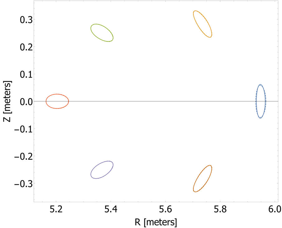
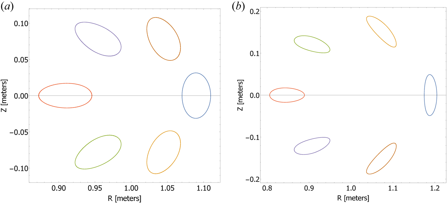
The accuracy of the fit is evident from the plot of the poloidal cross-sections. As seen in figure 2, there are only very slight differences between the VMEC and fitted cross-sections. These differences are negligible for the plots of the poloidal cross-sections of the quasisymmetric stellarators shown in figure 3.

Figure 2.

The poloidal cross-sections of W7-X. There are dashed and solid lines for the near-axis and VMEC cross-sections, respectively, but the differences are nearly indistinguishable.

Figure 3.

(a) The poloidal cross-sections of the fitted quasi-axisymmetric stellarator. (b) The poloidal cross-sections of the fitted quasi-helically symmetric stellarator. There are dashed and solid lines for the near-axis and VMEC cross-sections, respectively, but the differences are almost indistinguishable.

While there are very few visual discrepancies between the VMEC surfaces and the near-axis fits, we again note that near the axis, only $\psi _2$ is needed to accurately describe the surface (Jorge et al. Reference Jorge, Sengupta and Landreman2020b). Because $\psi _3$ is in (3.7), slight visual discrepancies in the third-order fit may lead to larger discrepancies in the magnetic well. This motivates the need for a more direct way to calculate higher order surface coefficients.

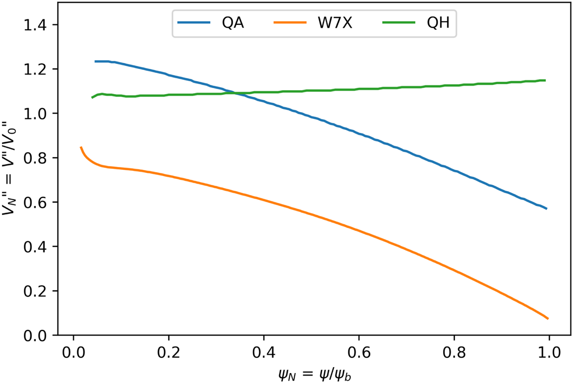
In figure 4, we plot the quantity $V_N'' = V''/V_0''$ as a function of the normalized toroidal flux, where $V''$ is the magnetic well calculated by VMEC and $V_0''$ is the magnetic well calculated from (3.7). The W7-X equilibrium is the same, but for the two quasisymmetric stellarators, we choose boundary surfaces further from the axis, with $\psi _b \sim 0.003\ \textrm {T} \ \textrm {m}^{2}$. For the quasisymmetric stellarators, even further from the axis ($\psi _N = 0.5$), the near-axis magnetic well remains approximately within 20 % of the VMEC magnetic well. We note that these surfaces represent a minor radius of approximately 0.1 m, and that similar discrepancies are found in figure 1 of Landreman & Jorge (Reference Landreman and Jorge2020). The discrepancies are larger for the W7-X equilibrium because its boundary surface is significantly further from the axis. Finally, the first several VMEC surfaces for each design were excluded because the magnetic well calculated by VMEC changed very rapidly near the axis and so are more inaccurate.

Figure 4.

The ratio of the VMEC and near-axis magnetic well $V_N'' = V''/V_0''$ plotted over the normalized toroidal flux. The W7-X equilibrium is the same as in figure 1, but the quasisymmetric equilibria have boundary surfaces further from the axis.

Finally, after fitting the plasma parameters describing the quasi-axisymmetric stellarator equilibrium from figure 1 for several of its surfaces, we numerically solve the system of equations in (4.9) and (4.10), and then evaluate the integral in (4.15). We then calculate the magnetic well and use (4.16) to sum all the terms to calculate Mercier's criterion to the lowest order. In figure 5, we compare our results for the lowest order criterion to the value of $D_{\textrm {Merc}}$ from VMEC. We can see that at smaller minor radii, the two results are very similar, but they diverge at larger radii. We note that at the largest radii $a = 0.1\ \textrm {m}$, the expansion parameter $\epsilon \sim 0.18$.

Figure 5.

The lowest order criterion calculated from the near-axis expansion and the value of $D_{\textrm {Merc}}$ from VMEC. Each point represents a configuration evaluated at the boundary at different aspect ratios.