1 Introduction
The accumulation of woody debris around bridge piers in rivers has long been the object of significant concerns among engineers and scientists. Debris jams modify the flow field around the piers, leading to deeper and larger scour holes (Melville and Dongol Reference Melville and Dongol1992; Pagliara and Carnacina Reference Pagliara and Carnacina2011), increased hydrodynamic loadings exerted onto the pier structure and increased upstream water levels. The first two effects have been widely held responsible for the collapse of many bridges around the world (Diehl Reference Diehl1997), while the third is often acknowledged as a key factor influencing the risk of flooding. In the past few decades, much research has been devoted towards determining the influence of debris accumulations on the above effects (Melville and Dongol Reference Melville and Dongol1992; Pagliara and Carnacina Reference Pagliara and Carnacina2011; Schmocker and Hager Reference Schmocker and Hager2013; Gschnitzer et al. Reference Gschnitzer, Gems, Mazzorana and Aufleger2017; Ebrahimi et al. Reference Ebrahimi, Kripakaran, Prodanovic, Kahraman, Riella, Tabor, Arthur and Djordević2018). Numerous field observations have also been made, which have generically described the typical shape of debris jams as an inverted half-cone (Abbe and Montgomery Reference Abbe and Montgomery1996; Diehl Reference Diehl1997). However, less attention has been given to understanding the processes governing the actual formation of these debris accumulations, or their subsequent removal from a pier by the flow. Such an understanding is key for improving our ability to model the effects of debris on the stability of bridges and flooding. In particular, predicting the dimensions and shape of woody debris jams that can possibly be formed at given bridges is an essential step towards this goal.
Debris accumulations are formed by large trees being trapped at bridge piers (Diehl Reference Diehl1997; Lagasse et al. Reference Lagasse, Colopper, Zevenbergen, Spitz and Girard2010), and previous studies indicated that the entrapment of individual debris elements depends on the approach flow velocity (Bocchiola, Rulli & Rosso Reference Bocchiola, Rulli and Rosso2008). This obstruction initiates a process of self-assembly whereby other floating debris elements transported by the flow build a framework that collects debris of various sizes, leading to the gradual growth of the accumulation (Manners, Doyle & Small Reference Manners, Doyle and Small2007; Manners and Doyle Reference Manners and Doyle2008). A recent study by Panici and de Almeida (Reference Panici and de Almeida2018) reproduced the processes of formation and growth of woody debris accumulations at bridge piers in a laboratory flume under turbulent flow ( $Re$ ranging from
 $5\times 10^{4}$ to
 $3\times 10^{5}$). These experiments showed that after the successive collection of individual debris pieces, all debris accumulations reach a critical stage at which point they rotate en masse about the pier and are dislodged by the flow (a condition hereafter referred to as failure). In many instances, an oscillatory rotational motion was observed prior to the dislodgement. These experiments also confirmed previous field observations by Diehl (Reference Diehl1997) and Lagasse et al. (Reference Lagasse, Colopper, Zevenbergen, Spitz and Girard2010) that debris jams formed at piers take the shape of half-conical porous bodies. Data from Panici and de Almeida (Reference Panici and de Almeida2018) showed that prior to failure, all debris accumulations display a certain degree of asymmetry relative to the vertical pivot axis. The maximum jam size, expressed by width
 $W$, height
 $H$ and length
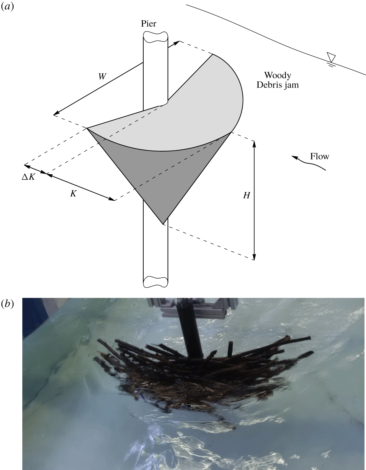
 $K$ (as shown in figure 1), is of primary importance for engineering design. Data from Panici and de Almeida (Reference Panici and de Almeida2018) showed that these maximum dimensions typically coincide with the onset of the final oscillatory or rotational stage leading to failure. Despite the extensive experimental observations, the underlying physical processes responsible for jam failure have not been systematically investigated.
(a) Sketch of a debris jam at a bridge pier, including its geometrical characteristics and (b) an example of a woody debris jam from experiments by Panici and de Almeida (Reference Panici and de Almeida2018) – view from upstream of the pier.

In this paper, we test the hypothesis that the main characteristics of the motion of debris jams observed by Panici and de Almeida (Reference Panici and de Almeida2018) can be captured by a simple fluid–debris interaction model based on shifts of the point of application of drag. The derivation of the model describing the fluid–debris interaction is detailed in § 2, which results in a set of ordinary differential equations. The fixed points of this system are analysed in § 3, which provides insights into the main parameters governing the stability of debris jams. A phase-plane analysis of the model is presented in § 4. A comparison against laboratory observations is provided in § 5.
2 Model construction
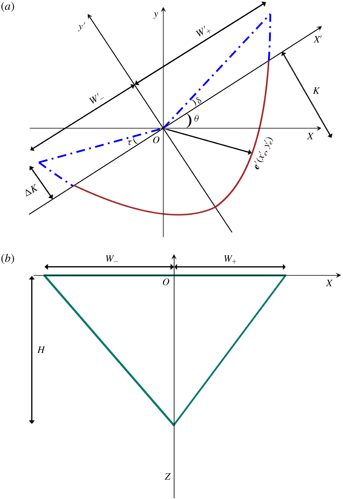
Consider the problem of the rotational motion of a porous half-conical body, assumed of uniform porosity, about a cylinder immersed in a predominantly unidirectional free-surface turbulent flow field. Further, we assume that the diameter of the cylinder is negligible compared to the size of the body, so that the position of the pivot point is assumed not to change with the motion of the body (i.e. the contact between the body and the cylinder occurs along a vertical line). The geometry of the body, which generically reproduces the main characteristics observed by Panici and de Almeida (Reference Panici and de Almeida2018), is described by the width  $W$ in the direction normal to the main flow, a longitudinal length
 $K$ and a depth
 $H$ below the water surface, as shown in figure 2. In addition, the dimension
 $\unicode[STIX]{x0394}K$ is introduced to represent the downstream extension beyond the pivot point (hereafter referred to as the tail). For simplicity, the tail length
 $\unicode[STIX]{x0394}K$ is assumed equal on both sides.
Conceptualised geometry of a debris jam at a pier. (a) The plan view and (b) the maximum projected area of the jam for a given angle of rotation  $\unicode[STIX]{x1D703}$.

To describe the motion of the solid, we adopt two Cartesian frames of reference. In the first frame,  $x$,
 $y$ and
 $z$ denote the transverse, streamwise and vertical coordinates, respectively. The second frame is defined by the coordinates
 $x^{\prime }$,
 $y^{\prime }$ and
 $z^{\prime }$ and is used to describe a rotation
 $\unicode[STIX]{x1D703}$ of the first frame about the vertical axis (
 $z=z^{\prime }$). The coordinates of the edge of the debris body are denoted by
 $x_{e}$,
 $y_{e}$ and
 $z_{e}$ (or
 $x_{e}^{\prime }$,
 $y_{e}^{\prime }$ and
 $z_{e}^{\prime }$ for the second frame of reference). A shape asymmetry is introduced by the condition
 $W_{-}^{\prime }<W_{+}^{\prime }$ (figure 2). The rotational motion of the debris jam about the vertical axis can be modelled by the principle of conservation of angular momentum
 $I\ddot{\unicode[STIX]{x1D703}}=\unicode[STIX]{x1D6E4}$, where
 $I$ is the moment of inertia of the debris body with respect to the axis of rotation
 $z$ (which must include the added mass effect) and
 $\unicode[STIX]{x1D6E4}$ is the torque of all external forces applied to the debris body. The proposed model assumes that drag
 $F_{D}=0.5\unicode[STIX]{x1D70C}C_{D}Av^{2}$, which is also assumed parallel to the streamwise direction, is the dominant force governing the rotational motion, where
 $\unicode[STIX]{x1D70C}$ is the water density,
 $A$ is the frontal area of the solid projected onto the
 $x{-}z$ plane,
 $v$ is a time-averaged characteristic velocity (e.g. free-stream mean velocity) and
 $C_{D}$ is the corresponding coefficient of drag, which may depend on several geometric, fluid or flow properties. Since the diameter of the cylinder is assumed negligible, it follows that the torque of the force due to friction between the body and the cylinder is zero. Other forces that take part in this process, such as the hydrostatic force difference between the upstream and downstream sides of the solid or the lift force, are neglected in the proposed model. Whilst flow in rivers is inherently turbulent, the model does not include fluctuations of the hydrodynamic force due to turbulence. In addition, it is assumed that drag is applied at the centroid of the cross-sectional area
 $A$. In essence, it is therefore postulated that the rotational motion is mainly governed by variations of the torque of drag induced by changes in
 $A$ and the
 $x$ position of its centroid
 $x_{c}$, which occur as a function of
 $\unicode[STIX]{x1D703}$ and the geometry of the solid (e.g.
 $W_{+}^{\prime }$,
 $W_{-}^{\prime }$,
 $K$,
 $\unicode[STIX]{x0394}K$), which yields
 $$\begin{eqnarray}I\ddot{\unicode[STIX]{x1D703}}=F_{D}x_{c}={\textstyle \frac{1}{2}}\unicode[STIX]{x1D70C}C_{D}Av^{2}x_{c}.\end{eqnarray}$$
Equation (2.1) implies that for  $\unicode[STIX]{x1D703}=0$, a perfectly symmetric solid (
 $W_{-}^{\prime }=W_{+}^{\prime }$) would remain static (
 $\unicode[STIX]{x1D6E4}=0$). From this stable condition, any asymmetry (i.e.
 $W_{-}^{\prime }<W_{+}^{\prime }$) or small rotation
 $\unicode[STIX]{x1D703}$ would lead to
 $x_{c}\neq 0$ and initiate a flow–solid dynamic interaction.
The geometry of the debris body (figure 2b) is modelled by a piecewise second-order polynomial describing the position  $e^{\prime }=[x_{e}^{\prime },y_{e}^{\prime }]$ of the leading (i.e. upstream) boundary of the body at the free surface:
 $$\begin{eqnarray}\displaystyle \left.\begin{array}{@{}c@{}}y_{e}^{\prime }={\displaystyle \frac{K+\unicode[STIX]{x0394}K}{W_{-}^{\prime 2}}}x_{e}^{\prime 2}-K,\quad \text{for}~x_{e}^{\prime }\in \left(0,~\pm W_{-}^{\prime }\right),\\ y_{e}^{\prime }={\displaystyle \frac{K+\unicode[STIX]{x0394}K}{W_{+}^{\prime 2}}}x_{e}^{\prime 2}-K,\quad \text{for}~x_{e}^{\prime }\in \left(0,~\pm W_{+}^{\prime }\right),\end{array}\right\} & & \displaystyle\end{eqnarray}$$
To account for the effect of asymmetry, we introduce the asymmetry factor defined as
 $$\begin{eqnarray}\unicode[STIX]{x1D713}=\frac{W_{+}^{\prime }}{W_{-}^{\prime }}.\end{eqnarray}$$
Therefore, horizontal planar asymmetry (i.e.  $W_{+}^{\prime }>W_{-}^{\prime }$) implies
 $\unicode[STIX]{x1D713}>1$. Considering that
 $W_{+}^{\prime }+W_{-}^{\prime }=W$,
 $W_{-}^{\prime }=W/(1+\unicode[STIX]{x1D713})$ and
 $W_{+}^{\prime }=W\unicode[STIX]{x1D713}/(1+\unicode[STIX]{x1D713})$, yields
 $$\begin{eqnarray}\displaystyle \left.\begin{array}{@{}c@{}}y_{e}^{\prime }={\displaystyle \frac{\left(K+\unicode[STIX]{x0394}K\right)\left(1+\unicode[STIX]{x1D713}\right)^{2}}{W^{2}}}{x^{\prime }}_{e}^{2}-K,\quad \text{for}~x_{e}^{\prime }\in \left(0,~\pm W_{-}^{\prime }\right),\\ y_{e}^{\prime }={\displaystyle \frac{\left(K+\unicode[STIX]{x0394}K\right)\left(1+\unicode[STIX]{x1D713}\right)^{2}}{W^{2}\unicode[STIX]{x1D713}^{2}}}{x^{\prime }}_{e}^{2}-K,\quad \text{for}~x_{e}^{\prime }\in \left(0,~\pm W_{+}^{\prime }\right).\end{array}\right\} & & \displaystyle\end{eqnarray}$$
Two dimensionless variables  $\unicode[STIX]{x1D6FC}=W/K$ and
 $\unicode[STIX]{x1D6FD}=\unicode[STIX]{x0394}K/K$ are introduced to describe the shape of the debris body and the relative size of the tail. Substituting
 $\unicode[STIX]{x1D6FC}$ and
 $\unicode[STIX]{x1D6FD}$ into (2.4) yields
 $$\begin{eqnarray}\displaystyle \left.\begin{array}{@{}c@{}}y_{e}^{\prime }={\displaystyle \frac{\left(1+\unicode[STIX]{x1D6FD}\right)\left(1+\unicode[STIX]{x1D713}\right)^{2}}{\unicode[STIX]{x1D6FC}W}}{x^{\prime }}_{e}^{2}-{\displaystyle \frac{W}{\unicode[STIX]{x1D6FC}}},\quad \text{for}~x_{e}^{\prime }\in \left(0,~\pm W_{-}^{\prime }\right),\\ y_{e}^{\prime }={\displaystyle \frac{\left(1+\unicode[STIX]{x1D6FD}\right)\left(1+\unicode[STIX]{x1D713}\right)^{2}}{\unicode[STIX]{x1D6FC}W\unicode[STIX]{x1D713}^{2}}}{x^{\prime }}_{e}^{2}-{\displaystyle \frac{W}{\unicode[STIX]{x1D6FC}}},\quad \text{for}~x_{e}^{\prime }\in \left(0,~\pm W_{+}^{\prime }\right).\end{array}\right\} & & \displaystyle\end{eqnarray}$$
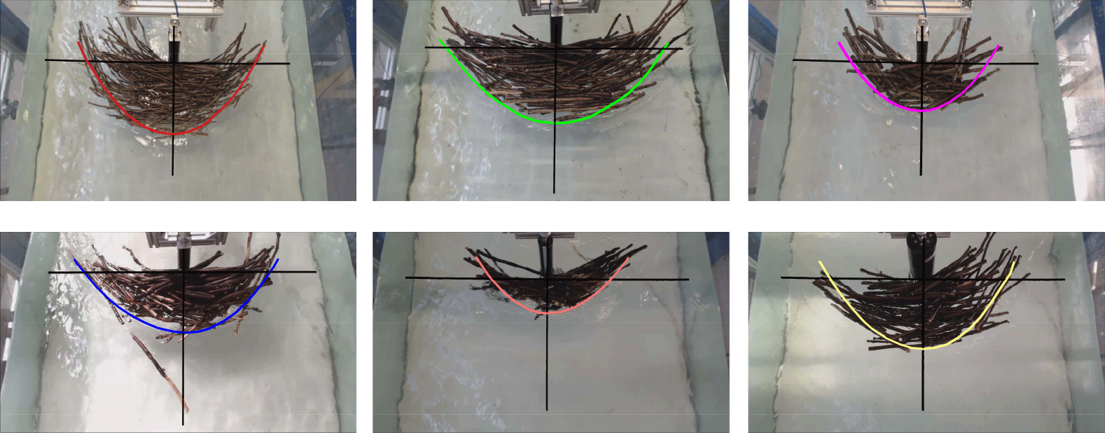
Examples of the curves used to model the shapes of the accumulations. Each background image shows debris accumulation obtained during the experiments by Panici and de Almeida (Reference Panici and de Almeida2018). The pier–jam contact point represents the origin of the  $x$ and
 $y$ axes (solid black lines) as sketched in figure 2.

Figure 3 shows examples of how (2.5) can model the top geometry of debris jams formed at the laboratory scale. Equation (2.5) is here used to define the expressions for the area  $A$, centroid
 $x_{c}$ and moment of inertia
 $I$. Since
 $A$ and
 $x_{c}$ depend on the projection of
 $\boldsymbol{e}^{\prime }$ onto the
 $x{-}z$ plane (see figure 2), they change with the rotation of the debris body. These expressions are given by (details of the derivations are provided in appendix A)
 $$\begin{eqnarray}A=\left\{\begin{array}{@{}ll@{}}{\displaystyle \frac{WH}{2}}\!\left[{\displaystyle \frac{\unicode[STIX]{x1D6FC}}{4\left(\unicode[STIX]{x1D713}+1\right)^{2}\left(1+\unicode[STIX]{x1D6FD}\right)}}{\displaystyle \frac{\cos ^{2}\unicode[STIX]{x1D703}}{\text{sin}\unicode[STIX]{x1D703}}}+{\displaystyle \frac{\text{sin}\unicode[STIX]{x1D703}}{\unicode[STIX]{x1D6FC}}}+{\displaystyle \frac{\unicode[STIX]{x1D713}}{\unicode[STIX]{x1D713}+1}}{\displaystyle \frac{\cos \left(\unicode[STIX]{x1D703}+\unicode[STIX]{x1D6FF}\right)}{\cos \left(\unicode[STIX]{x1D6FF}\right)}}\right],\quad & \!\!\!\text{for }-{\displaystyle \frac{\unicode[STIX]{x03C0}}{2}}\leqslant \unicode[STIX]{x1D703}<\unicode[STIX]{x1D703}_{t}^{-},\\ {\displaystyle \frac{WH}{2\left(\unicode[STIX]{x1D713}+1\right)}}\left[\unicode[STIX]{x1D713}{\displaystyle \frac{\cos \left(\unicode[STIX]{x1D703}+\unicode[STIX]{x1D6FF}\right)}{\cos \left(\unicode[STIX]{x1D6FF}\right)}}+{\displaystyle \frac{\cos \left(\unicode[STIX]{x1D703}-\unicode[STIX]{x1D70F}\right)}{\cos \left(\unicode[STIX]{x1D70F}\right)}}\right],\quad & \!\!\!\text{for }\unicode[STIX]{x1D703}_{t}^{-}\leqslant \unicode[STIX]{x1D703}\leqslant \unicode[STIX]{x1D703}_{t}^{+},\\ {\displaystyle \frac{WH}{2}}\left[{\displaystyle \frac{\unicode[STIX]{x1D6FC}\unicode[STIX]{x1D713}^{2}}{4\left(\unicode[STIX]{x1D713}+1\right)^{2}\left(1+\unicode[STIX]{x1D6FD}\right)}}{\displaystyle \frac{\cos ^{2}\unicode[STIX]{x1D703}}{\text{sin}\unicode[STIX]{x1D703}}}+{\displaystyle \frac{\text{sin}\unicode[STIX]{x1D703}}{\unicode[STIX]{x1D6FC}}}+{\displaystyle \frac{1}{\unicode[STIX]{x1D713}+1}}{\displaystyle \frac{\cos \left(\unicode[STIX]{x1D703}-\unicode[STIX]{x1D70F}\right)}{\cos \left(\unicode[STIX]{x1D70F}\right)}}\right],\quad & \!\!\!\text{for }\unicode[STIX]{x1D703}_{t}^{+}<\unicode[STIX]{x1D703}\leqslant {\displaystyle \frac{\unicode[STIX]{x03C0}}{2}}\end{array}\right.\end{eqnarray}$$
and
 $$\begin{eqnarray}x_{c}=\left\{\begin{array}{@{}ll@{}}{\displaystyle \frac{W}{3}}\left[{\displaystyle \frac{\unicode[STIX]{x1D713}}{\unicode[STIX]{x1D713}+1}}{\displaystyle \frac{\cos \left(\unicode[STIX]{x1D703}+\unicode[STIX]{x1D6FF}\right)}{\cos \left(\unicode[STIX]{x1D6FF}\right)}}-{\displaystyle \frac{\unicode[STIX]{x1D6FC}}{4\left(\unicode[STIX]{x1D713}+1\right)^{2}\left(1+\unicode[STIX]{x1D6FD}\right)}}{\displaystyle \frac{\cos ^{2}\unicode[STIX]{x1D703}}{\text{sin}\unicode[STIX]{x1D703}}}-{\displaystyle \frac{\text{sin}\unicode[STIX]{x1D703}}{\unicode[STIX]{x1D6FC}}}\right],\quad & \text{for }-{\displaystyle \frac{\unicode[STIX]{x03C0}}{2}}\leqslant \unicode[STIX]{x1D703}<\unicode[STIX]{x1D703}_{t}^{-},\\ {\displaystyle \frac{W}{3\left(\unicode[STIX]{x1D713}+1\right)}}\left[\unicode[STIX]{x1D713}{\displaystyle \frac{\cos \left(\unicode[STIX]{x1D703}+\unicode[STIX]{x1D6FF}\right)}{\cos \left(\unicode[STIX]{x1D6FF}\right)}}-{\displaystyle \frac{\cos \left(\unicode[STIX]{x1D703}-\unicode[STIX]{x1D70F}\right)}{\cos \left(\unicode[STIX]{x1D70F}\right)}}\right],\quad & \text{for }\unicode[STIX]{x1D703}_{t}^{-}\leqslant \unicode[STIX]{x1D703}\leqslant \unicode[STIX]{x1D703}_{t}^{+},\\ {\displaystyle \frac{W}{3}}\left[{\displaystyle \frac{\unicode[STIX]{x1D6FC}\unicode[STIX]{x1D713}^{2}}{4\left(\unicode[STIX]{x1D713}+1\right)^{2}\left(1+\unicode[STIX]{x1D6FD}\right)}}{\displaystyle \frac{\cos ^{2}\unicode[STIX]{x1D703}}{\text{sin}\unicode[STIX]{x1D703}}}+{\displaystyle \frac{\text{sin}\unicode[STIX]{x1D703}}{\unicode[STIX]{x1D6FC}}}-{\displaystyle \frac{1}{\unicode[STIX]{x1D713}+1}}{\displaystyle \frac{\cos \left(\unicode[STIX]{x1D703}-\unicode[STIX]{x1D70F}\right)}{\cos \left(\unicode[STIX]{x1D70F}\right)}}\right],\quad & \text{for }\unicode[STIX]{x1D703}_{t}^{+}<\unicode[STIX]{x1D703}\leqslant {\displaystyle \frac{\unicode[STIX]{x03C0}}{2}},\end{array}\right.\end{eqnarray}$$
where  $\unicode[STIX]{x1D6FF}$ and
 $\unicode[STIX]{x1D70F}$ are the angles between the tail edge and the
 $x^{\prime }$ axis, as shown in figure 2, and
 $\unicode[STIX]{x1D703}_{t}^{+}$ and
 $\unicode[STIX]{x1D703}_{t}^{-}$ (defined in appendix A) are angles defining the sub-domains of the piecewise functions above. The moment of inertia
 $I$ also includes the added mass effect, as outlined in appendix A. For simplicity, some terms that are assumed independent of time (which include the dimensions of the solid and the time-averaged characteristic velocity) are grouped into a single parameter:
 $$\begin{eqnarray}\unicode[STIX]{x1D712}=\frac{1}{12}\frac{\unicode[STIX]{x1D70C}C_{D}W^{2}Hv^{2}}{I}.\end{eqnarray}$$
The dependency of the coefficient of drag on the orientation of the body is neglected here (although it may be readily included for problems in which the relation is known), so that  $C_{D}$ is assumed independent of time in (2.8). Substituting equations (2.6), (2.7) and (2.8) into (2.1) and defining
 $\unicode[STIX]{x1D714}=\dot{\unicode[STIX]{x1D703}}$, yields the following system of equations:
 $$\begin{eqnarray}\displaystyle & & \displaystyle \displaystyle \qquad \quad \dot{\unicode[STIX]{x1D703}}=\unicode[STIX]{x1D714},\nonumber\\ \displaystyle & & \displaystyle \displaystyle \dot{\unicode[STIX]{x1D714}}=\left\{\begin{array}{@{}l@{}}\unicode[STIX]{x1D712}\left[\left({\displaystyle \frac{\unicode[STIX]{x1D713}}{\unicode[STIX]{x1D713}+1}}{\displaystyle \frac{\cos \left(\unicode[STIX]{x1D703}+\unicode[STIX]{x1D6FF}\right)}{\cos \unicode[STIX]{x1D6FF}}}\right)^{2}-\left({\displaystyle \frac{\unicode[STIX]{x1D6FC}}{4\left(1+\unicode[STIX]{x1D6FD}\right)\left(1+\unicode[STIX]{x1D713}\right)^{2}}}{\displaystyle \frac{\cos ^{2}\unicode[STIX]{x1D703}}{\text{sin}\unicode[STIX]{x1D703}}}+{\displaystyle \frac{\text{sin}\unicode[STIX]{x1D703}}{\unicode[STIX]{x1D6FC}}}\right)^{2}\right],\quad \\ \qquad \qquad \text{for }-{\displaystyle \frac{\unicode[STIX]{x03C0}}{2}}\leqslant \unicode[STIX]{x1D703}<\unicode[STIX]{x1D703}_{t}^{-},\quad \\ {\displaystyle \frac{\unicode[STIX]{x1D712}}{\left(\unicode[STIX]{x1D713}+1\right)^{2}}}\left[\unicode[STIX]{x1D713}^{2}{\displaystyle \frac{\cos ^{2}\left(\unicode[STIX]{x1D703}+\unicode[STIX]{x1D6FF}\right)}{\cos ^{2}\left(\unicode[STIX]{x1D6FF}\right)}}-{\displaystyle \frac{\cos ^{2}\left(\unicode[STIX]{x1D703}-\unicode[STIX]{x1D70F}\right)}{\cos ^{2}\left(\unicode[STIX]{x1D70F}\right)}}\right],\quad \\ \qquad \qquad \text{for }\unicode[STIX]{x1D703}_{t}^{-}\leqslant \unicode[STIX]{x1D703}\leqslant \unicode[STIX]{x1D703}_{t}^{+},\quad \\ \unicode[STIX]{x1D712}\left[\left({\displaystyle \frac{\unicode[STIX]{x1D6FC}\unicode[STIX]{x1D713}^{2}}{4\left(1+\unicode[STIX]{x1D6FD}\right)\left(1+\unicode[STIX]{x1D713}\right)^{2}}}{\displaystyle \frac{\cos ^{2}\unicode[STIX]{x1D703}}{\text{sin}\unicode[STIX]{x1D703}}}+{\displaystyle \frac{\text{sin}\unicode[STIX]{x1D703}}{\unicode[STIX]{x1D6FC}}}\right)^{2}-\left({\displaystyle \frac{1}{1+\unicode[STIX]{x1D713}}}{\displaystyle \frac{\cos \left(\unicode[STIX]{x1D703}-\unicode[STIX]{x1D70F}\right)}{\cos \unicode[STIX]{x1D70F}}}\right)^{2}\right],\quad \\ \qquad \qquad \text{for }\unicode[STIX]{x1D703}_{t}^{+}<\unicode[STIX]{x1D703}\leqslant {\displaystyle \frac{\unicode[STIX]{x03C0}}{2}}.\quad \end{array}\right.\nonumber\\ \displaystyle & & \displaystyle\end{eqnarray}$$
Equations (2.9) will be used to model the rotational motion of the solid in the range  $-\unicode[STIX]{x03C0}/2\leqslant \unicode[STIX]{x1D703}\leqslant \unicode[STIX]{x03C0}/2$. The phase-plane object of the following analysis has coordinates
 $\unicode[STIX]{x1D703}$,
 $\unicode[STIX]{x1D714}$.
3 Analysis of fixed points
3.1 Non-tailed accumulation
This section analyses the fixed points of equation (2.9) for the particular condition given by  $\unicode[STIX]{x1D6FD}=0$ (that is, a half-cone body with no tails, i.e.
 $\unicode[STIX]{x0394}K=0$). Under this condition, equation (2.9) simplifies to
 $$\begin{eqnarray}\displaystyle & & \displaystyle \displaystyle \qquad \quad \dot{\unicode[STIX]{x1D703}}=\unicode[STIX]{x1D714},\nonumber\\ \displaystyle & & \displaystyle \displaystyle \dot{\unicode[STIX]{x1D714}}=\left\{\begin{array}{@{}l@{}}\unicode[STIX]{x1D712}\left[\left({\displaystyle \frac{\unicode[STIX]{x1D713}}{1+\unicode[STIX]{x1D713}}}\cos \unicode[STIX]{x1D703}\right)^{2}-\left({\displaystyle \frac{\unicode[STIX]{x1D6FC}}{4\left(1+\unicode[STIX]{x1D713}\right)^{2}}}{\displaystyle \frac{\cos ^{2}\unicode[STIX]{x1D703}}{\text{sin}\unicode[STIX]{x1D703}}}+{\displaystyle \frac{\text{sin}\unicode[STIX]{x1D703}}{\unicode[STIX]{x1D6FC}}}\right)^{2}\right],\quad \\ \qquad \qquad \text{for }-\unicode[STIX]{x03C0}/2\leqslant \unicode[STIX]{x1D703}<\unicode[STIX]{x1D703}_{t}^{-},\quad \\ \unicode[STIX]{x1D712}{\displaystyle \frac{\unicode[STIX]{x1D713}-1}{\unicode[STIX]{x1D713}+1}}\cos ^{2}\unicode[STIX]{x1D703}\quad \text{for }\unicode[STIX]{x1D703}_{t}^{-}\leqslant \unicode[STIX]{x1D703}\leqslant \unicode[STIX]{x1D703}_{t}^{+},\quad \\ \unicode[STIX]{x1D712}\left[\left({\displaystyle \frac{\unicode[STIX]{x1D6FC}\unicode[STIX]{x1D713}^{2}}{4\left(1+\unicode[STIX]{x1D713}\right)^{2}}}{\displaystyle \frac{\cos ^{2}\unicode[STIX]{x1D703}}{\text{sin}\unicode[STIX]{x1D703}}}+{\displaystyle \frac{\text{sin}\unicode[STIX]{x1D703}}{\unicode[STIX]{x1D6FC}}}\right)^{2}-\left({\displaystyle \frac{1}{1+\unicode[STIX]{x1D713}}}\cos \unicode[STIX]{x1D703}\right)^{2}\right],\quad \\ \qquad \qquad \text{for }\unicode[STIX]{x1D703}_{t}^{+}<\unicode[STIX]{x1D703}\leqslant {\displaystyle \frac{\unicode[STIX]{x03C0}}{2}}.\quad \end{array}\right.\end{eqnarray}$$
We first determine the fixed points of the system (3.1). Within the sub-domain  $\unicode[STIX]{x1D703}_{t}^{-}\leqslant \unicode[STIX]{x1D703}\leqslant \unicode[STIX]{x1D703}_{t}^{+}$, equation (3.1) only admits one fixed point at (
 $\unicode[STIX]{x03C0}/2$, 0). This is, however, outside the sub-domain within which the function is defined (i.e.
 $\unicode[STIX]{x1D703}_{t}^{+}$ is always less than
 $\unicode[STIX]{x03C0}/2$). Therefore no fixed points are found within this region of the phase plane. Regarding the sub-domain
 $\unicode[STIX]{x1D703}_{t}^{+}<\unicode[STIX]{x1D703}\leqslant \unicode[STIX]{x03C0}/2$, four solutions for (3.1) set equal to zero are found at
 $\unicode[STIX]{x1D714}=0$ and
 $\unicode[STIX]{x1D703}=\text{arctan}(\unicode[STIX]{x1D6FC}(\pm 1\pm \sqrt{1-\unicode[STIX]{x1D713}^{2}}/2(1+\unicode[STIX]{x1D713})))$. However, none of these points are real, since
 $\unicode[STIX]{x1D713}>1$ by definition. It follows that no fixed points are found in the interval
 $\unicode[STIX]{x1D703}_{t}^{+}<\unicode[STIX]{x1D703}\leqslant \unicode[STIX]{x03C0}/2$.
In the sub-domain  $-\unicode[STIX]{x03C0}/2\leqslant \unicode[STIX]{x1D703}<\unicode[STIX]{x1D703}_{t}^{-}$,
 $[\dot{\unicode[STIX]{x1D703}},\dot{\unicode[STIX]{x1D714}}]=0$ (from (3.1)) admits four solutions given by
 $\unicode[STIX]{x1D714}=0$ and
 $\unicode[STIX]{x1D703}=\text{arctan}(\unicode[STIX]{x1D6FC}(\pm \unicode[STIX]{x1D713}\pm \sqrt{\unicode[STIX]{x1D713}^{2}-1}/2(1+\unicode[STIX]{x1D713})))$. Two of these solutions cannot be accepted as they would result in a positive value of
 $\unicode[STIX]{x1D703}$, and hence outside of the sub-domain of study, being
 $\unicode[STIX]{x1D703}_{t}^{-}<0$ (i.e. from (A 7)) for any conditions. For the other two solutions, one of them will always be larger than
 $\unicode[STIX]{x1D703}_{t}^{-}$ and cannot be accepted for the domain of study. Within the sub-domain
 $-\unicode[STIX]{x03C0}/2\leqslant \unicode[STIX]{x1D703}<\unicode[STIX]{x1D703}_{t}^{-}$, only one fixed point is found at
 $\unicode[STIX]{x1D714}=0$ and
 $$\begin{eqnarray}\unicode[STIX]{x1D703}_{nt}=\text{arctan}\left(-\unicode[STIX]{x1D6FC}\frac{\unicode[STIX]{x1D713}+\sqrt{\unicode[STIX]{x1D713}^{2}-1}}{2\left(1+\unicode[STIX]{x1D713}\right)}\right).\end{eqnarray}$$
The nature of this fixed point can be determined by analysing the eigenvalues  $\unicode[STIX]{x1D706}_{nt}$ of the Jacobian
 $J_{nt}$ of (3.1) at the fixed point
 $\unicode[STIX]{x1D703}_{nt}$ (where the subscript
 $nt$ is used to denote the specific condition of a non-tailed body):
 $$\begin{eqnarray}\displaystyle & \displaystyle J_{nt}=\left[\begin{array}{@{}cc@{}}0 & 1\\ 2\unicode[STIX]{x1D712}\!\left[-\text{sin}\left(2\unicode[STIX]{x1D703}_{nt}\right){\displaystyle \frac{\unicode[STIX]{x1D713}^{2}}{\left(\unicode[STIX]{x1D713}+1\right)^{2}}}-{\displaystyle \frac{2\left(1+\!\left({\displaystyle \frac{\unicode[STIX]{x1D6FC}^{2}}{4\left(\unicode[STIX]{x1D713}+1\right)^{2}}}-1\right)\cos ^{2}\unicode[STIX]{x1D703}_{nt}\right)^{2}}{\unicode[STIX]{x1D6FC}^{2}\text{sin}^{3}\unicode[STIX]{x1D703}_{nt}}}\right] & 0\end{array}\right],\qquad & \displaystyle\end{eqnarray}$$
 $$\begin{eqnarray}\displaystyle & \displaystyle \unicode[STIX]{x1D706}_{nt}=\pm \sqrt{2\unicode[STIX]{x1D712}}\sqrt{-\text{sin}\left(2\unicode[STIX]{x1D703}_{nt}\right)\frac{\unicode[STIX]{x1D713}^{2}}{\left(\unicode[STIX]{x1D713}+1\right)^{2}}-\frac{2\left(1+\!\left({\displaystyle \frac{\unicode[STIX]{x1D6FC}^{2}}{4\left(\unicode[STIX]{x1D713}+1\right)^{2}}}-1\right)\cos ^{2}\unicode[STIX]{x1D703}_{nt}\right)^{2}}{\unicode[STIX]{x1D6FC}^{2}\text{sin}^{3}\unicode[STIX]{x1D703}_{nt}}}.\qquad & \displaystyle\end{eqnarray}$$
Since  $\unicode[STIX]{x1D703}_{nt}$ is always negative, the term inside the square root of (3.4) must be positive, resulting in real and distinct eigenvalues. Thus, the fixed point
 $\unicode[STIX]{x1D703}_{nt}$ is a saddle. Saddle nodes are surrounded by open trajectories except along the stable manifold. Therefore, considering the original real-world problem of a body immersed in a turbulent flow where instantaneous fluctuations in the magnitude and point of application of the drag force occur, the problem of a non-tailed accumulation can be practically assumed as inherently unstable.
3.2 Tailed accumulations
In this section we show that other fixed points emerge for values of  $\unicode[STIX]{x1D6FD}>0$ by analysing the system (2.9). A fixed point for the sub-domain
 $\unicode[STIX]{x1D703}_{t}^{-}\leqslant \unicode[STIX]{x1D703}\leqslant \unicode[STIX]{x1D703}_{t}^{+}$ of (2.9) occurs at
 $\unicode[STIX]{x1D714}=0$ and
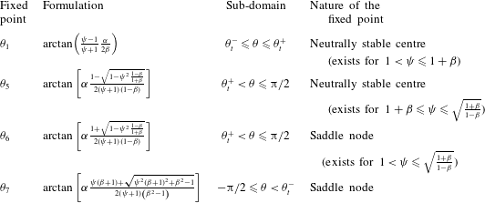
 $$\begin{eqnarray}\unicode[STIX]{x1D703}_{1}=\text{arctan}\left(\frac{\unicode[STIX]{x1D713}-1}{\unicode[STIX]{x1D713}+1}\frac{\unicode[STIX]{x1D6FC}}{2\unicode[STIX]{x1D6FD}}\right).\end{eqnarray}$$
Since  $\unicode[STIX]{x1D703}_{1}\leqslant \unicode[STIX]{x1D703}_{t}^{+}$ and considering (A 7), it follows that for
 $\unicode[STIX]{x1D703}_{1}$ to exist a necessary condition is
 $$\begin{eqnarray}\unicode[STIX]{x1D713}\leqslant 1+\unicode[STIX]{x1D6FD}.\end{eqnarray}$$
A second solution of (2.9) equal to 0 at  $\unicode[STIX]{x1D703}_{2}=\unicode[STIX]{x03C0}/2$ is omitted as it falls outside the sub-domain considered here. It is now possible to analyse the nature of the fixed point
 $\unicode[STIX]{x1D703}_{1}$. The Jacobian of (2.9) for
 $\unicode[STIX]{x1D703}_{t}^{-}\leqslant \unicode[STIX]{x1D703}\leqslant \unicode[STIX]{x1D703}_{t}^{+}$ and at the fixed point
 $\unicode[STIX]{x1D703}=\unicode[STIX]{x1D703}_{1}$ is given by
 $$\begin{eqnarray}J_{1}=\left[\begin{array}{@{}cc@{}}0 & 1\\ -{\displaystyle \frac{2\unicode[STIX]{x1D712}}{\left(\unicode[STIX]{x1D713}+1\right)^{2}}}\left[\unicode[STIX]{x1D713}^{2}{\displaystyle \frac{\text{sin}\left(2\left(\unicode[STIX]{x1D703}_{1}+\unicode[STIX]{x1D6FF}\right)\right)}{\cos ^{2}\unicode[STIX]{x1D6FF}}}-{\displaystyle \frac{\text{sin}\left(2\left(\unicode[STIX]{x1D703}_{1}-\unicode[STIX]{x1D70F}\right)\right)}{\cos ^{2}\unicode[STIX]{x1D70F}}}\right] & 0\\ \end{array}\right],\end{eqnarray}$$
the eigenvalues of which are
 $$\begin{eqnarray}\unicode[STIX]{x1D706}_{1}=\pm \sqrt{-\frac{2\unicode[STIX]{x1D712}}{\left(\unicode[STIX]{x1D713}+1\right)^{2}}\left[\unicode[STIX]{x1D713}^{2}\frac{\text{sin}\left(2\left(\unicode[STIX]{x1D703}_{1}+\unicode[STIX]{x1D6FF}\right)\right)}{\cos ^{2}\unicode[STIX]{x1D6FF}}-\frac{\text{sin}\left(2\left(\unicode[STIX]{x1D703}_{1}-\unicode[STIX]{x1D70F}\right)\right)}{\cos ^{2}\left(\unicode[STIX]{x1D70F}\right)}\right]}.\end{eqnarray}$$
The sign of the terms inside the square brackets defines the nature of the fixed points in the phase plane. If positive,  $\unicode[STIX]{x1D706}_{1}$ is purely imaginary, and hence the fixed point is a neutrally stable centre; if negative,
 $\unicode[STIX]{x1D706}_{1}$ has two real and opposite values and the fixed point is a saddle (i.e. unstable node). For the case of
 $\unicode[STIX]{x1D706}_{1}$, the term within square brackets is always positive; hence, the eigenvalue is purely imaginary. As a result, the fixed point
 $\unicode[STIX]{x1D703}_{1}$ will always be a neutrally stable centre.
For the interval  $\unicode[STIX]{x1D703}_{t}^{+}<\unicode[STIX]{x1D703}\leqslant \unicode[STIX]{x03C0}/2$, the same analysis reveals four additional solutions of equation (2.9) set equal to zero at
 $\unicode[STIX]{x1D714}=0$ and
 $$\begin{eqnarray}\displaystyle \left.\begin{array}{@{}c@{}}\unicode[STIX]{x1D703}_{3}=-\text{arctan}\left[\unicode[STIX]{x1D6FC}{\displaystyle \frac{1-\sqrt{1-\unicode[STIX]{x1D713}^{2}}}{2\left(\unicode[STIX]{x1D713}+1\right)\left(1+\unicode[STIX]{x1D6FD}\right)}}\right],\\ \unicode[STIX]{x1D703}_{4}=-\text{arctan}\left[\unicode[STIX]{x1D6FC}{\displaystyle \frac{1+\sqrt{1-\unicode[STIX]{x1D713}^{2}}}{2\left(\unicode[STIX]{x1D713}+1\right)\left(1+\unicode[STIX]{x1D6FD}\right)}}\right],\\ \unicode[STIX]{x1D703}_{5}=\text{arctan}\left[\unicode[STIX]{x1D6FC}{\displaystyle \frac{1-\sqrt{1-\unicode[STIX]{x1D713}^{2}{\displaystyle \frac{1-\unicode[STIX]{x1D6FD}}{1+\unicode[STIX]{x1D6FD}}}}}{2\left(\unicode[STIX]{x1D713}+1\right)\left(1-\unicode[STIX]{x1D6FD}\right)}}\right],\\ \unicode[STIX]{x1D703}_{6}=\text{arctan}\left[\unicode[STIX]{x1D6FC}{\displaystyle \frac{1+\sqrt{1-\unicode[STIX]{x1D713}^{2}{\displaystyle \frac{1-\unicode[STIX]{x1D6FD}}{1+\unicode[STIX]{x1D6FD}}}}}{2\left(\unicode[STIX]{x1D713}+1\right)\left(1-\unicode[STIX]{x1D6FD}\right)}}\right].\end{array}\right\} & & \displaystyle\end{eqnarray}$$
Since  $\unicode[STIX]{x1D713}>1$,
 $\unicode[STIX]{x1D703}_{3}$ and
 $\unicode[STIX]{x1D703}_{4}$ are not real and cannot be fixed points of (2.9). On the other hand,
 $\unicode[STIX]{x1D703}_{5}$ and
 $\unicode[STIX]{x1D703}_{6}$ are real only if
 $1-\unicode[STIX]{x1D713}^{2}(1-\unicode[STIX]{x1D6FD})/(1+\unicode[STIX]{x1D6FD})\geqslant 0$. As a result, the fixed points
 $\unicode[STIX]{x1D703}_{5}$ and
 $\unicode[STIX]{x1D703}_{6}$ can only exist in the phase plane if
 $$\begin{eqnarray}\unicode[STIX]{x1D6FD}\geqslant \frac{\unicode[STIX]{x1D713}^{2}-1}{\unicode[STIX]{x1D713}^{2}+1}\end{eqnarray}$$
or, alternatively,
 $$\begin{eqnarray}1<\unicode[STIX]{x1D713}^{2}\leqslant \frac{1+\unicode[STIX]{x1D6FD}}{1-\unicode[STIX]{x1D6FD}}.\end{eqnarray}$$
In other words,  $\unicode[STIX]{x1D703}_{5}$ and
 $\unicode[STIX]{x1D703}_{6}$ can only exist for values of
 $\unicode[STIX]{x1D6FD}<1$ (i.e.
 $\unicode[STIX]{x0394}K<K$). In addition, the fixed points
 $\unicode[STIX]{x1D703}_{5}$ and
 $\unicode[STIX]{x1D703}_{6}$ must satisfy the condition
 $\unicode[STIX]{x1D703}_{5,6}\geqslant \unicode[STIX]{x1D703}_{t}^{+}$. First,
 $\unicode[STIX]{x1D703}_{t}^{+}\leqslant \unicode[STIX]{x1D703}_{6}$ can be simplified as
 $$\begin{eqnarray}\frac{1}{\unicode[STIX]{x1D713}}\unicode[STIX]{x1D713}^{2}\frac{1-\unicode[STIX]{x1D6FD}}{1+\unicode[STIX]{x1D6FD}}\leqslant 1+\sqrt{1-\unicode[STIX]{x1D713}^{2}\frac{1-\unicode[STIX]{x1D6FD}}{1+\unicode[STIX]{x1D6FD}}}.\end{eqnarray}$$
The second term on the right-hand side of (3.12) is real only if  $\unicode[STIX]{x1D713}^{2}(1-\unicode[STIX]{x1D6FD})/(1+\unicode[STIX]{x1D6FD})\leqslant 1$. Therefore, the left-hand side is always less than 1 (since, by definition,
 $\unicode[STIX]{x1D713}>1$), while the right-hand side must be greater than 1; hence,
 $\unicode[STIX]{x1D703}_{6}>\unicode[STIX]{x1D703}_{t}^{+}$ in any case. The condition
 $\unicode[STIX]{x1D703}_{5}\geqslant \unicode[STIX]{x1D703}_{t}^{+}$ leads to
 $\unicode[STIX]{x1D713}\geqslant 1+\unicode[STIX]{x1D6FD}$. As
 $\unicode[STIX]{x1D703}_{1}$ is only defined for
 $\unicode[STIX]{x1D713}\leqslant \unicode[STIX]{x1D6FD}+1$, it follows that
 $\unicode[STIX]{x1D703}_{1}$ and
 $\unicode[STIX]{x1D703}_{5}$ cannot coexist in the phase plane, resulting in a maximum of two fixed points (i.e.
 $\unicode[STIX]{x1D703}_{6}$ and either
 $\unicode[STIX]{x1D703}_{5}$ or
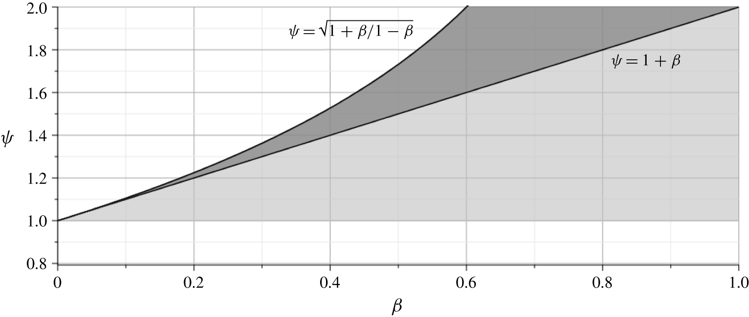
 $\unicode[STIX]{x1D703}_{1}$) in the positive domain. Figure 4 shows the region of existence of
 $\unicode[STIX]{x1D703}_{5}$ and
 $\unicode[STIX]{x1D703}_{6}$ for values of
 $\unicode[STIX]{x1D713}$ and
 $\unicode[STIX]{x1D6FD}$. When conditions in (3.10) or (3.11) are not satisfied, neither
 $\unicode[STIX]{x1D703}_{5}$ nor
 $\unicode[STIX]{x1D703}_{6}$ exists in the phase plane, and thus there will only be open trajectories. Practically, this implies that a small tail or a very large asymmetry factor would lead to a rotation that eventually causes the failure of the debris body. On the right-hand end of the figure, for values of
 $\unicode[STIX]{x1D6FD}>1$, neither
 $\unicode[STIX]{x1D703}_{5}$ nor
 $\unicode[STIX]{x1D703}_{6}$ exists, and there will only be
 $\unicode[STIX]{x1D703}_{1}$ which (if neutrally stable) would result in a highly stable situation for any condition.
Region of existence for  $\unicode[STIX]{x1D703}_{5}$ and
 $\unicode[STIX]{x1D703}_{6}$: the former is found only in the darker area (which corresponds to the non-existence of
 $\unicode[STIX]{x1D703}_{1}$), while the latter is defined for both darker and lighter shaded areas. Values of
 $\unicode[STIX]{x1D713}$ and
 $\unicode[STIX]{x1D6FD}$ outside of this region would result in no fixed points
 $\unicode[STIX]{x1D703}_{5}$ and
 $\unicode[STIX]{x1D703}_{6}$.

To understand the nature of  $\unicode[STIX]{x1D703}_{5}$ and
 $\unicode[STIX]{x1D703}_{6}$, we analyse the eigenvalues of the Jacobian matrix of (2.9) within the sub-domain
 $\unicode[STIX]{x1D703}_{t}^{+}<\unicode[STIX]{x1D703}\leqslant \unicode[STIX]{x03C0}/2$:
 $$\begin{eqnarray}J_{2}=\left[\begin{array}{@{}cc@{}}0 & 1\\ 2\unicode[STIX]{x1D712}\left[{\displaystyle \frac{\text{sin}\left(2\left(\unicode[STIX]{x1D703}_{5,6}-\unicode[STIX]{x1D70F}\right)\right)}{\cos ^{2}\unicode[STIX]{x1D70F}\left(\unicode[STIX]{x1D713}+1\right)^{2}}}+{\displaystyle \frac{2\left(1+\left({\displaystyle \frac{\unicode[STIX]{x1D6FC}^{2}\unicode[STIX]{x1D713}^{2}}{4\left(1+\unicode[STIX]{x1D6FD}\right)\left(\unicode[STIX]{x1D713}+1\right)^{2}}}-1\right)\cos ^{2}\unicode[STIX]{x1D703}_{5,6}\right)^{2}}{\unicode[STIX]{x1D6FC}^{2}\text{sin}^{3}\unicode[STIX]{x1D703}_{5,6}}}\right] & 0\\ \end{array}\right],\end{eqnarray}$$
for which case  $\unicode[STIX]{x1D703}$ can be either
 $\unicode[STIX]{x1D703}_{5}$ or
 $\unicode[STIX]{x1D703}_{6}$. The resulting eigenvalues are
 $$\begin{eqnarray}\unicode[STIX]{x1D706}_{2}=\pm \sqrt{2\unicode[STIX]{x1D712}}\sqrt{\frac{\text{sin}\left(2\left(\unicode[STIX]{x1D703}_{5,6}-\unicode[STIX]{x1D70F}\right)\right)}{\cos ^{2}\unicode[STIX]{x1D70F}\left(\unicode[STIX]{x1D713}+1\right)^{2}}+\frac{2\left(1+\left({\displaystyle \frac{\unicode[STIX]{x1D6FC}^{2}\unicode[STIX]{x1D713}^{2}}{4\left(1+\unicode[STIX]{x1D6FD}\right)\left(\unicode[STIX]{x1D713}+1\right)^{2}}}-1\right)\cos ^{2}\unicode[STIX]{x1D703}_{5,6}\right)^{2}}{\unicode[STIX]{x1D6FC}^{2}\text{sin}^{3}\unicode[STIX]{x1D703}_{5,6}}}.\end{eqnarray}$$
Equation (3.14) shows that  $\unicode[STIX]{x1D706}_{2}$ can be either real or imaginary, depending on the sign of
 $\text{sin}(2(\unicode[STIX]{x1D703}_{5,6}-\unicode[STIX]{x1D70F}))$. For values of
 $\unicode[STIX]{x1D703}_{5,6}$ sufficiently large (e.g.
 $\unicode[STIX]{x1D703}_{5,6}\geqslant \unicode[STIX]{x1D70F}$),
 $\unicode[STIX]{x1D706}_{2}$ could be real, resulting in a saddle point, otherwise a neutrally stable centre is observed. This results in the alternation between a centre and a saddle, as will be observed in the phase-plane analysis presented in § 4, whereby
 $\unicode[STIX]{x1D703}_{1}$ (or
 $\unicode[STIX]{x1D703}_{5}$ depending on
 $\unicode[STIX]{x1D6FD}$) provides a centre, while
 $\unicode[STIX]{x1D703}_{6}$ is a saddle.
Finally, for the interval  $-\unicode[STIX]{x03C0}/2\leqslant \unicode[STIX]{x1D703}<\unicode[STIX]{x1D703}_{t}^{-}$, solutions to (2.9) set equal to zero occur at
 $\unicode[STIX]{x1D714}=0$ and
 $$\begin{eqnarray}\displaystyle \left.\begin{array}{@{}c@{}}\displaystyle \unicode[STIX]{x1D703}_{7}=\text{arctan}\left[\unicode[STIX]{x1D6FC}\frac{\unicode[STIX]{x1D713}\left(\unicode[STIX]{x1D6FD}+1\right)+\sqrt{\unicode[STIX]{x1D713}^{2}\left(\unicode[STIX]{x1D6FD}+1\right)^{2}+\unicode[STIX]{x1D6FD}^{2}-1}}{2\left(\unicode[STIX]{x1D713}+1\right)\left(\unicode[STIX]{x1D6FD}^{2}-1\right)}\right],\\ \displaystyle \unicode[STIX]{x1D703}_{8}=\text{arctan}\left[\unicode[STIX]{x1D6FC}\frac{\unicode[STIX]{x1D713}\left(\unicode[STIX]{x1D6FD}+1\right)-\sqrt{\unicode[STIX]{x1D713}^{2}\left(\unicode[STIX]{x1D6FD}+1\right)^{2}+\unicode[STIX]{x1D6FD}^{2}-1}}{2\left(\unicode[STIX]{x1D713}+1\right)\left(\unicode[STIX]{x1D6FD}^{2}-1\right)}\right],\\ \displaystyle \unicode[STIX]{x1D703}_{9}=\text{arctan}\left[\unicode[STIX]{x1D6FC}\frac{\unicode[STIX]{x1D713}-\sqrt{\unicode[STIX]{x1D713}^{2}-1}}{2\left(\unicode[STIX]{x1D713}+1\right)\left(1+\unicode[STIX]{x1D6FD}\right)}\right],\\ \displaystyle \unicode[STIX]{x1D703}_{10}=\text{arctan}\left[\unicode[STIX]{x1D6FC}\frac{\unicode[STIX]{x1D713}+\sqrt{\unicode[STIX]{x1D713}^{2}-1}}{2\left(\unicode[STIX]{x1D713}+1\right)\left(1+\unicode[STIX]{x1D6FD}\right)}\right].\end{array}\right\} & & \displaystyle\end{eqnarray}$$
The two results for  $\unicode[STIX]{x1D703}_{9}$ and
 $\unicode[STIX]{x1D703}_{10}$ will be positive; hence, these will not be part of the sub-domain. On the other hand, both
 $\unicode[STIX]{x1D703}_{7}$ and
 $\unicode[STIX]{x1D703}_{8}$ will be negative for
 $\unicode[STIX]{x1D6FD}<1$. Comparing
 $\unicode[STIX]{x1D703}_{7}$ with
 $\unicode[STIX]{x1D703}_{t}^{-}$, the former will always be smaller than the latter, and thus a fixed point of the system; conversely,
 $\unicode[STIX]{x1D703}_{8}$ will always be greater than
 $\unicode[STIX]{x1D703}_{t}^{-}$, and thus not included in the sub-domain. This is the analogous situation to the non-tailed case analysed in the previous section. In order to understand the nature of the only fixed point
 $\unicode[STIX]{x1D703}_{7}$, we analyse the Jacobian of (2.9) within the sub-domain
 $-\unicode[STIX]{x03C0}/2\leqslant \unicode[STIX]{x1D703}<\unicode[STIX]{x1D703}_{t}^{+}$:
 $$\begin{eqnarray}J_{3}=\left[\begin{array}{@{}cc@{}}0 & 1\\ 2\unicode[STIX]{x1D712}\left[-{\displaystyle \frac{\text{sin}\left(2\left(\unicode[STIX]{x1D703}_{7}+\unicode[STIX]{x1D6FF}\right)\right)}{\cos ^{2}\unicode[STIX]{x1D6FF}}}{\displaystyle \frac{\unicode[STIX]{x1D713}^{2}}{\left(\unicode[STIX]{x1D713}+1\right)^{2}}}-{\displaystyle \frac{2\left(1+\left({\displaystyle \frac{\unicode[STIX]{x1D6FC}^{2}}{4\left(1+\unicode[STIX]{x1D6FD}\right)\left(\unicode[STIX]{x1D713}+1\right)^{2}}}-1\right)\cos ^{2}\unicode[STIX]{x1D703}_{7}\right)^{2}}{\unicode[STIX]{x1D6FC}^{2}\text{sin}^{3}\unicode[STIX]{x1D703}_{7}}}\right] & 0\end{array}\right].\end{eqnarray}$$
The resulting eigenvalues are
 $$\begin{eqnarray}\unicode[STIX]{x1D706}_{3}=\pm \sqrt{2\unicode[STIX]{x1D712}}\sqrt{-\frac{\text{sin}\left(2\left(\unicode[STIX]{x1D703}_{7}+\unicode[STIX]{x1D6FF}\right)\right)}{\cos ^{2}\unicode[STIX]{x1D6FF}}\frac{\unicode[STIX]{x1D713}^{2}}{\left(\unicode[STIX]{x1D713}+1\right)^{2}}-\frac{2\left(\!1+\left({\displaystyle \frac{\unicode[STIX]{x1D6FC}^{2}}{4\left(1+\unicode[STIX]{x1D6FD}\right)\left(\unicode[STIX]{x1D713}+1\!\right)^{2}}}-1\!\right)\cos ^{2}\unicode[STIX]{x1D703}_{7}\!\right)^{2}}{\unicode[STIX]{x1D6FC}^{2}\text{sin}^{3}\unicode[STIX]{x1D703}_{7}}}.\end{eqnarray}$$
In consideration that  $\unicode[STIX]{x1D703}_{7}$ is always negative, the term inside the square root in (3.17) will always be positive, and thus the eigenvalues are distinct and real, which will result in a saddle in the phase plane.
Table 1 provides a summary of the fixed points discussed above for the model of a tailed accumulation.
Summary of fixed points for the model of the tailed accumulation.

4 Phase-plane analysis
In this section, we analyse the phase plane of the system of differential equations discussed in the previous section to provide further insights into the behaviour of the proposed model.
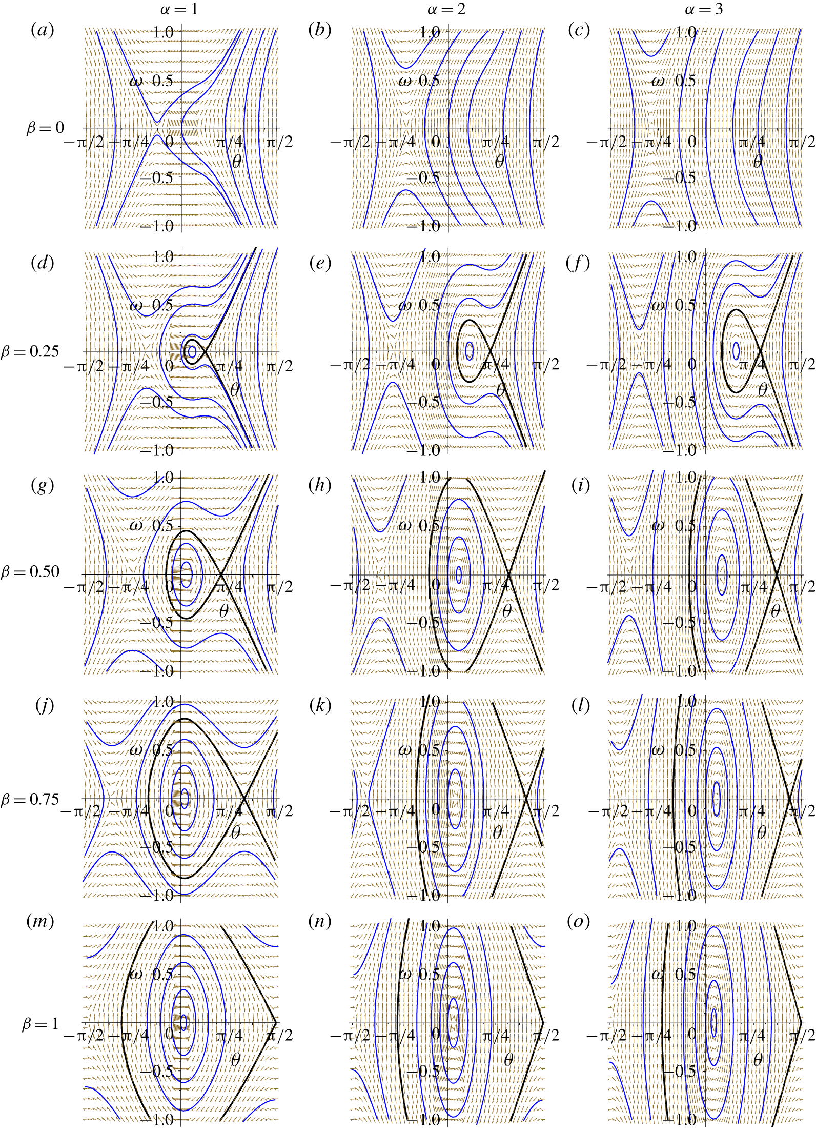
Phase portraits for constant  $\unicode[STIX]{x1D713}=1.20$ and varying
 $\unicode[STIX]{x1D6FC}$ and
 $\unicode[STIX]{x1D6FD}$. Horizontally,
 $\unicode[STIX]{x1D6FC}$ takes values of 1.0 (
 $a$,
 $d$,
 $g$,
 $j$,
 $m$), 2.0 (
 $b$,
 $e$,
 $h$,
 $k$,
 $n$) and 3.0 (
 $c$,
 $f$,
 $i$,
 $l$,
 $o$) from left to right. Vertically,
 $\unicode[STIX]{x1D6FD}$ takes values of 0 (
 $a$,
 $b$,
 $c$), 0.25 (
 $d$,
 $e$,
 $f$), 0.50 (
 $g$,
 $h$,
 $i$), 0.75 (
 $j$,
 $k$,
 $l$) and
 $1$ (
 $m$,
 $n$,
 $o$) from top to bottom.

Figure 5 shows different phase portraits plotted for a constant value of the asymmetry factor  $\unicode[STIX]{x1D713}=1.2,1\leqslant \unicode[STIX]{x1D6FC}\leqslant 3$ and
 $0\leqslant \unicode[STIX]{x1D6FD}\leqslant 1$. The blue lines in this figure represent arbitrary trajectories, whereas the black solid line is the boundary between stable (i.e. orbits around the first fixed point) and unstable (i.e. open trajectories) solutions. These phase portraits were plotted for particular values of other intervening parameters, namely
 $W=0.6~\text{m}$,
 $H=0.15~\text{m}$,
 $\unicode[STIX]{x1D70C}_{j}=800~\text{kg}~\text{m}^{-3}$,
 $C_{D}=1.5$ and
 $v=0.4~\text{m}~\text{s}^{-1}$. These values are within the range tested in the experiments by Panici and de Almeida (Reference Panici and de Almeida2018), and are adopted here in order to enable an analysis of the proposed model under conditions for which evidence is available. The value of
 $\unicode[STIX]{x1D70C}_{j}$ adopted here was approximated using the value of the coefficient of added mass of
 $C_{M}=1.0$. Panels in the top row of figure 5 depict the condition analysed in § 3.1, where
 $\unicode[STIX]{x1D6FD}=0$ and only open trajectories are possible, except for the stable manifold of the saddle in the negative domain. For
 $\unicode[STIX]{x1D6FD}>0$, two fixed points emerge in the positive domain (namely a centre and a saddle), as also discussed previously. The size of closed orbits about the neutrally stable centre increases with the value of
 $\unicode[STIX]{x1D6FD}$, which translates into increased stability of the system. Furthermore, for increasing
 $\unicode[STIX]{x1D6FD}$ the distance on the
 $\unicode[STIX]{x1D703}$ axis between these two fixed points increases: the first fixed point (i.e. the neutrally stable centre) is shifted towards the origin, whilst the second fixed point (i.e. the saddle) moves towards higher values of
 $\unicode[STIX]{x1D703}$. This increases the chances of an oscillatory motion being stable even when the values of the angular displacements are large. At the highest range of
 $\unicode[STIX]{x1D6FD}$, very large angles and/or angular velocities would be needed in order to reach open trajectories leading to the failure of the debris jam. The value of
 $\unicode[STIX]{x1D6FD}=1$ is used to illustrate the extreme case of a jam with a very large tail, in which case a strong stability is observed. Indeed, the model implies that for
 $\unicode[STIX]{x1D6FD}=1$, it would be possible to observe a rotation approaching
 $\unicode[STIX]{x1D703}=\unicode[STIX]{x03C0}/2$ that would remain in oscillatory motion about the pier. The figure also shows that when
 $\unicode[STIX]{x1D6FD}>0$, the stable area of the phase plane increases with
 $\unicode[STIX]{x1D6FC}$.
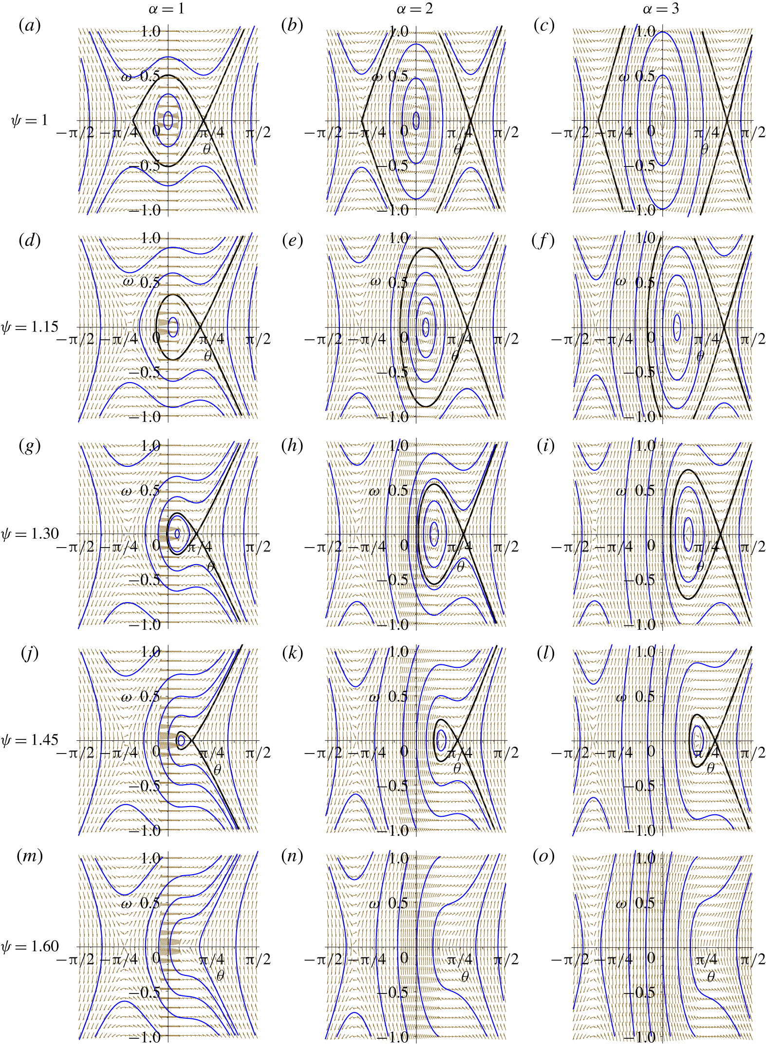
Figure 6 shows the phase portrait of the system (2.9) for a constant value of  $\unicode[STIX]{x1D6FD}=0.40$, and
 $\unicode[STIX]{x1D6FC}$ and
 $\unicode[STIX]{x1D713}$ varying within the ranges
 $1\leqslant \unicode[STIX]{x1D6FC}\leqslant 3$ and
 $1\leqslant \unicode[STIX]{x1D713}\leqslant 1.60$ (values of
 $W$,
 $H$,
 $\unicode[STIX]{x1D70C}_{j}$,
 $C_{D}$ and
 $v$ in this figure are the same as those used in figure 5). The panels in different rows are used to highlight the influence of asymmetry on the stability of the system. The top row shows the phase portrait for a perfectly symmetric body (
 $\unicode[STIX]{x1D713}=1$). Under this condition the stable centre is located at the origin, and it is observed that a large perturbation would need to be introduced to induce failure. In addition, the required perturbation from
 $\unicode[STIX]{x1D703}=0$ increases significantly with
 $\unicode[STIX]{x1D6FC}$, as has also been previously pointed out in figure 5. As
 $\unicode[STIX]{x1D713}$ increases, the two fixed points approach each other, reducing the region of the domain where closed orbits are possible. For
 $\unicode[STIX]{x1D713}=1.6$ the system is intrinsically unstable; no fixed points are observed and any small perturbation would eventually lead to a non-periodic motion. This occurs because
 $\unicode[STIX]{x1D713}$ is larger than the critical condition as observed in (3.11), which for
 $\unicode[STIX]{x1D6FD}=0.4$ is
 $\unicode[STIX]{x1D713}=1.53$.
The phase planes shown in figures 5 and 6 also reveal a saddle point in the negative side of the domain. This implies that, in theory, the body could reach an open trajectory towards negative values of  $\unicode[STIX]{x1D703}$, although this would require relatively large initial displacements, compared to those required for open trajectories along the positive side of the domain.
Phase portraits for constant  $\unicode[STIX]{x1D6FD}=0.40$ and varying
 $\unicode[STIX]{x1D713}$ and
 $\unicode[STIX]{x1D6FC}$. Horizontally,
 $\unicode[STIX]{x1D6FC}$ takes values of 1.0 (
 $a$,
 $d$,
 $g$,
 $j$,
 $m$), 2.0 (
 $b$,
 $e$,
 $h$,
 $k$,
 $n$) and 3.0 (
 $c$,
 $f$,
 $i$,
 $l$,
 $o$) from left to right. Vertically,
 $\unicode[STIX]{x1D713}$ takes values of 1 (
 $a$,
 $b$,
 $c$), 1.15 (
 $d$,
 $e$,
 $f$), 1.30 (
 $g$,
 $h$,
 $i$), 1.45 (
 $j$,
 $k$,
 $l$) and 1.60 (
 $m$,
 $n$,
 $o$) from top to bottom.

5 Comparison against experimental observations
In this section we compare the model predictions of stability against previous laboratory observations obtained at different stages during the growth of debris accumulations at a vertical cylinder immersed in a turbulent free-surface flow.
5.1 Impossibility of stability of non-tailed accumulations
We first test the ability of the proposed model to capture the impossibility of an accumulation remaining stable under the hypothetical condition of a non-tailed shape. During the 570 experiments of Panici and de Almeida (Reference Panici and de Almeida2018), such a shape was never observed, neither during a stable nor during a critical (i.e. immediately prior to failure) condition. The results of the analysis presented in § 3.1 confirm that the model agrees with these laboratory observations. Namely, no fixed points are possible in the positive domain of the phase plane. The only fixed point occurs for negative values of  $\unicode[STIX]{x1D703}$ and is a saddle node. While in theory stability occurs along the stable manifold of the saddle, in the real world any small disturbance from this state – e.g. induced by turbulence – would result in open trajectories. Therefore, in practical terms, such a system is always unstable, and any small perturbation (i.e. planar asymmetry
 $\unicode[STIX]{x1D713}\neq 1$) would result in large rotations ultimately leading to the removal of the jam from the pier. In this case, the force exerted by drag would neither establish a rotation that is periodical nor tend to a static equilibrium.
5.2 Shape characteristics of stable accumulations
Experimental datasets of Panici and de Almeida (Reference Panici and de Almeida2018) provide the opportunity to compare the shape characteristics (i.e.  $\unicode[STIX]{x1D6FC}$,
 $\unicode[STIX]{x1D6FD}$ and
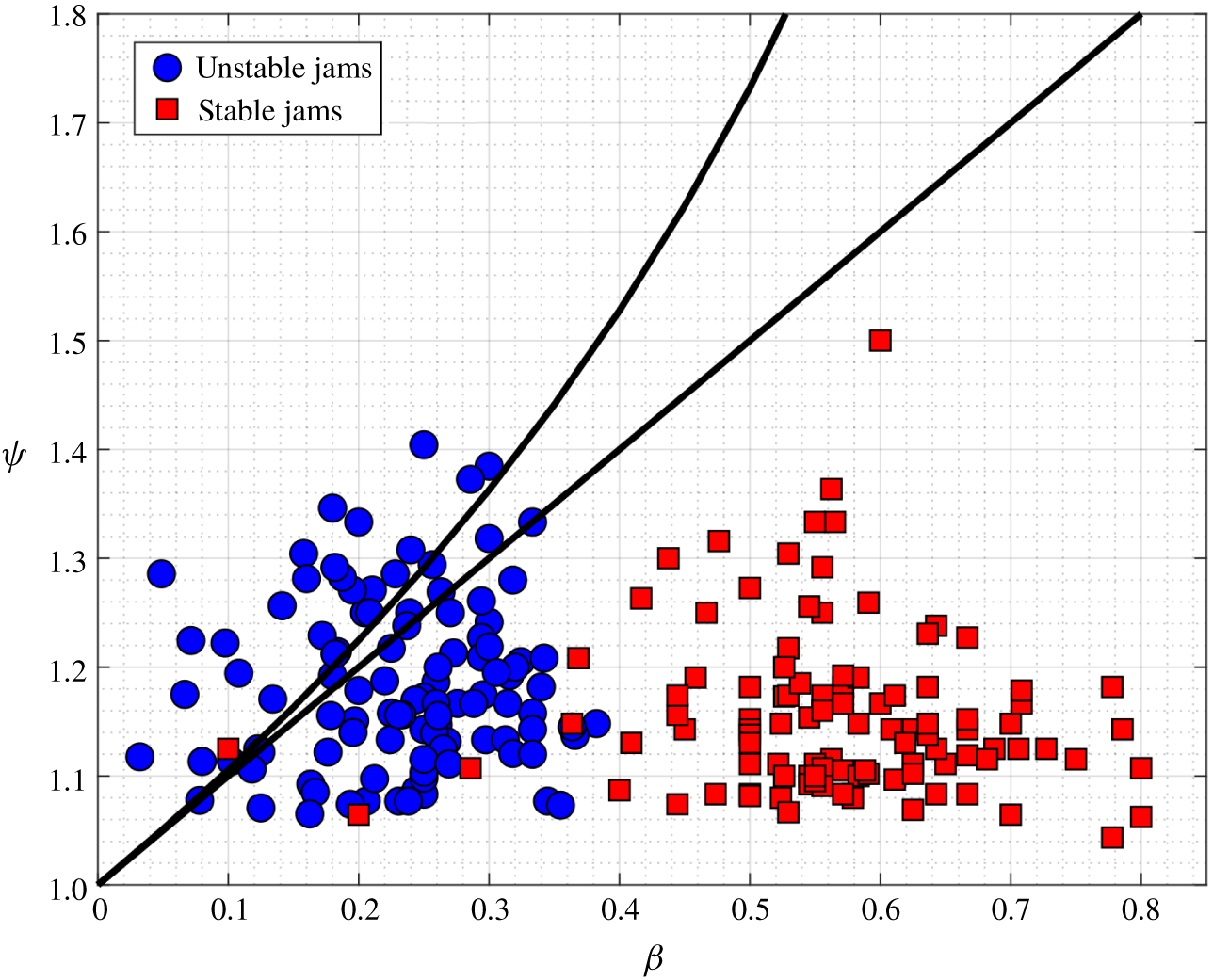
 $\unicode[STIX]{x1D713}$) of debris accumulations formed in the laboratory against the model’s predictions. Figure 7 shows the values of
 $\unicode[STIX]{x1D713}$ and
 $\unicode[STIX]{x1D6FD}$ observed during 105 different experiments, along with the curves defining the limits of existence of fixed points (as previously defined in figure 4). In this figure, the blue circles represent values of
 $\unicode[STIX]{x1D6FD}$ and
 $\unicode[STIX]{x1D713}$ at time
 $T$ immediately before the failure of the accumulation (that is, the elapsed time between the first piece of debris being entrapped and the beginning of the dislodgement of the whole debris jam), whereas the red squares represent the same values measured at
 $T/3$, when the body can be assumed stable (i.e. when very small or negligible periodical rotations were observed). The figure shows a clear distinction between the two groups. Stable jams are observed on the right-hand side of the graph, where the model predicts that both
 $\unicode[STIX]{x1D703}_{1}$ and
 $\unicode[STIX]{x1D703}_{6}$ exist and
 $\unicode[STIX]{x1D703}_{1}$ (i.e. the neutrally stable centre) is closer to the origin of the phase plane, which translates into high stability. On the other hand, unstable jams are found on the left-hand side of the graph, very close to the boundaries that define the existence of
 $\unicode[STIX]{x1D703}_{1}$ and
 $\unicode[STIX]{x1D703}_{5}$ and in many instances above the upper boundary, in which case no fixed points are found and only open trajectories are possible.
Region of existence of fixed points according to figure 4 overlapped with experimental data of Panici and de Almeida (Reference Panici and de Almeida2018).

5.3 Repeatability of observed dimensions at failure
The experiments of Panici and de Almeida (Reference Panici and de Almeida2018) showed that all debris piles, formed by the successive accumulation of individual debris elements, fail upon reaching maximum values of  $W$,
 $K$ and
 $H$. In addition, repeated experiments conducted under the same flow conditions showed that the dimensions at failure display a relatively small variation. At first, this last observation is somewhat puzzling, since the process of collection of debris elements is inherently stochastic. We here argue that such a behaviour can be explained based on the proposed model, as follows.
Section 4 has shown that the model predicts increasing stability with increasing values of  $\unicode[STIX]{x1D6FC}$ and
 $\unicode[STIX]{x1D6FD}$. This is in agreement with the process of accumulation of debris pieces observed in the laboratory by Panici and de Almeida (Reference Panici and de Almeida2018). Shortly after the first mesh of debris is formed, only a few debris elements are collected on the upstream side of the pier. The orientation of these elements is such that the initial values of
 $\unicode[STIX]{x0394}K$ and
 $W$ are large compared to the longitudinal dimension
 $K$, resulting in the maximum values for
 $\unicode[STIX]{x1D6FC}$ and
 $\unicode[STIX]{x1D6FD}$. Under these conditions, the model predicts a debris jam that is very stable, and experimental observations show that indeed no failure is observed during these initial stages. As other debris elements accumulate upstream, the growth rate of
 $K$ is faster than the corresponding growth of
 $W$ and
 $\unicode[STIX]{x0394}K$, and thus both
 $\unicode[STIX]{x1D6FC}$ and
 $\unicode[STIX]{x1D6FD}$ gradually decrease. Eventually, when the values of
 $\unicode[STIX]{x1D6FC}$ and
 $\unicode[STIX]{x1D6FD}$ are very low the jam is removed from the pier. The model predicts that low values of
 $\unicode[STIX]{x1D6FC}$ and
 $\unicode[STIX]{x1D6FD}$ result in a significant reduction of the stable region of the phase plane, thus increasing the probability of failure. This indicates that the condition in which failure occurs, while influenced by processes that are inherently stochastic, also has a strong deterministic component, which agrees with the repeatability of dimensions observed in various experiments.
5.4 Direction of failure
The phase portraits presented in § 4 show that open trajectories leading to a rotation towards the negative direction can be observed in the phase plane. For the body to follow this open trajectory, it must rotate by a certain negative value of  $\unicode[STIX]{x1D703}$ that depends on
 $\unicode[STIX]{x1D6FC}$,
 $\unicode[STIX]{x1D6FD}$ and
 $\unicode[STIX]{x1D713}$ (i.e.
 $\unicode[STIX]{x1D703}<\unicode[STIX]{x1D703}_{t}^{-}$). However, if the body is to reach these trajectories, it must first pass through a region of the domain filled with open positive trajectories, which would lead to a positive failure. In other words, failure by a rotation towards the side of the lowest semi-width is, in practice, virtually impossible. This agrees with the observations by Panici and de Almeida (Reference Panici and de Almeida2018), which show that all failures observed in 570 experiments occurred through a rotation towards the positive (i.e. widest side) direction.
6 Conclusions
In this paper we have proposed a modelling framework to analyse the interactions between flow and an immersed body that is free to rotate about a static vertical solid cylinder also immersed in the flow. The analysis was motivated by recent experiments performed by the authors to simulate the process of the collection of woody debris transported in rivers around bridge piers. In these experiments it was observed that formed jams can display an oscillatory rotational motion about the vertical cylinder, and that they are always ultimately removed from the cylinder by the flow. The proposed model was developed in order to understand these and other aspects of the observed behaviour. The development of the model was also aimed at improving our ability to describe the main parameters governing the formation of debris jams that can remain stable while exposed to flow over long periods. The model was built upon the assumption that the motion of the immersed body is primarily driven by dynamic changes of the point where drag force is applied, which in addition is assumed to depend on the geometry of the body and its orientation only. The geometry analysed in the paper, which aims to model the observed geometry of debris jams, was defined as an asymmetric half-cone with extensions that in the paper are referred to as tails.
The main geometrical variables of the model, namely the jam width  $W$, length
 $K$ and tail extension
 $\unicode[STIX]{x0394}K$, defined two dimensionless shape parameters
 $\unicode[STIX]{x1D6FC}=W/K$ and
 $\unicode[STIX]{x1D6FD}=\unicode[STIX]{x0394}K/K$, which along with an asymmetry factor
 $\unicode[STIX]{x1D713}$ were found to govern much of the observed behaviour. A nonlinear system of ordinary differential equations resulted from the application of conservation of angular momentum of the immersed body subject to the moment of the drag force. The system was analysed on the phase plane. For a tailed, asymmetric solid, three fixed points can be observed in the phase plane, which typically show alternation between a neutrally stable centre node and saddles. The dimensionless variables previously defined play key roles in the stability of the system (that is, the periodic rotation around the first fixed point). First, the tail factor
 $\unicode[STIX]{x1D6FD}$ is pivotal in order to provide stability. The model predicts that a non-tailed body (i.e.
 $\unicode[STIX]{x1D6FD}=0$) is inherently unstable, leading to open trajectories (i.e. a failure) even if it is almost perfectly symmetric. On the other hand, increasing values of
 $\unicode[STIX]{x1D6FD}$ produce more stable conditions by shifting the neutrally stable node towards the origin and the saddle towards higher values of
 $\unicode[STIX]{x1D703}$ (thus increasing the area of the phase plane corresponding to closed orbits). The asymmetry factor
 $\unicode[STIX]{x1D713}$ is also key to the stability of the system. For symmetric bodies (i.e.
 $\unicode[STIX]{x1D713}=1$), the neutrally stable node lies on the origin and only a very large perturbation could lead to a failure. On the other hand, if
 $\unicode[STIX]{x1D713}$ is greater than a threshold value (which also depends on
 $\unicode[STIX]{x1D6FD}$), the system is unconditionally unstable.
A comparison between experimental observations and model predictions confirmed the ability of the proposed model to capture the main characteristics of the motion of debris jams observed in the laboratory. This includes (i) the model’s prediction of the impossibility of a non-tailed body (which was never observed to form during 570 experiments) remaining stable; (ii) its ability to capture key differences in the shape of stable and unstable jams related to the values of  $\unicode[STIX]{x1D6FC}$,
 $\unicode[STIX]{x1D6FD}$ and
 $\unicode[STIX]{x1D713}$; (iii) an explanation for the repeatability of debris jam dimensions at failure; and (iv) the model’s prediction of the direction towards which the rotational motion leading to failure should occur, which agrees with all experimental data available. Whilst further validation of the proposed model for rotational oscillations of immersed bodies would require a detailed set of accurate experiments, the results obtained from our comparison against existing laboratory experiments are encouraging.
Acknowledgements
The authors are grateful for the financial support of the UK Engineering and Physical Sciences Research Council (EPSRC) through the Centre for Doctoral Training in Sustainable Infrastructure Systems (CDT-SIS), grant EP/L01582X/1.
Declaration of interests
The authors report no conflict of interest.
Appendix A
The area  $A$ and the position of its centroid
 $x_{c}$ are obtained by determining the maximum values of the projection
 $\boldsymbol{e}=\boldsymbol{R}\boldsymbol{e}^{\prime }$ of
 $\boldsymbol{e}^{\prime }$ onto the
 $x$ axis (herein referred to as
 $W_{-}$ and
 $W_{+}$, respectively) within the domain
 $-\unicode[STIX]{x03C0}/2\leqslant \unicode[STIX]{x1D703}\leqslant \unicode[STIX]{x03C0}/2$, where
 $\boldsymbol{R}$ is the rotation matrix and
 $\boldsymbol{e}^{\prime }$ is defined by (2.5). Since we are only interested in the first component of
 $\boldsymbol{e}$:
 $$\begin{eqnarray}x_{e}(x_{e}^{\prime },\unicode[STIX]{x1D703})=\left\{\begin{array}{@{}ll@{}}{x^{\prime }}_{e}\cos \unicode[STIX]{x1D703}-{\displaystyle \frac{\left(1+\unicode[STIX]{x1D6FD}\right)\left(1+\unicode[STIX]{x1D713}\right)^{2}}{\unicode[STIX]{x1D6FC}W}}{x^{\prime }}_{e}^{2}\text{sin}\unicode[STIX]{x1D703}+{\displaystyle \frac{W}{\unicode[STIX]{x1D6FC}}}\text{sin}\unicode[STIX]{x1D703},\quad & \text{for}~{x^{\prime }}_{e}\in \left(0,~\pm W_{-}^{\prime }\right),\\ {x^{\prime }}_{e}\cos \unicode[STIX]{x1D703}-{\displaystyle \frac{\left(1+\unicode[STIX]{x1D6FD}\right)\left(1+\unicode[STIX]{x1D713}\right)^{2}}{\unicode[STIX]{x1D6FC}W\unicode[STIX]{x1D713}^{2}}}{x^{\prime }}_{e}^{2}\text{sin}\unicode[STIX]{x1D703}+{\displaystyle \frac{W}{\unicode[STIX]{x1D6FC}}}\text{sin}\unicode[STIX]{x1D703},\quad & \text{for}~{x^{\prime }}_{e}\in \left(0,~\pm W_{+}^{\prime }\right).\end{array}\right.\end{eqnarray}$$
For low absolute values of the angle of rotation ( $\unicode[STIX]{x1D703}_{t}^{-}\leqslant \unicode[STIX]{x1D703}\leqslant \unicode[STIX]{x1D703}_{t}^{+}$), the optima of (A 1) given by
 $[W_{-},W_{+}]=[x_{e}(W_{-}^{\prime },\unicode[STIX]{x1D703}),x_{e}(W_{+}^{\prime },\unicode[STIX]{x1D703})]$, which for
 $W_{-}^{\prime }<W_{+}^{\prime }$ yields
 $$\begin{eqnarray}\displaystyle \left.\begin{array}{@{}c@{}}\displaystyle W_{-}(\unicode[STIX]{x1D703})=\frac{W}{\left(1+\unicode[STIX]{x1D713}\right)\cos \left(\unicode[STIX]{x1D70F}\right)}\cos \left(\unicode[STIX]{x1D703}-\unicode[STIX]{x1D70F}\right),\quad \text{for }\unicode[STIX]{x1D703}_{t}^{-}\leqslant \unicode[STIX]{x1D703}\leqslant \unicode[STIX]{x03C0}/2,\\ \displaystyle W_{+}(\unicode[STIX]{x1D703})=\frac{W\unicode[STIX]{x1D713}}{\left(1+\unicode[STIX]{x1D713}\right)\cos \left(\unicode[STIX]{x1D6FF}\right)}\cos \left(\unicode[STIX]{x1D703}+\unicode[STIX]{x1D6FF}\right),\quad \text{for }-\unicode[STIX]{x03C0}/2\leqslant \unicode[STIX]{x1D703}\leqslant \unicode[STIX]{x1D703}_{t}^{+},\end{array}\right\} & & \displaystyle\end{eqnarray}$$
where
 $$\begin{eqnarray}\displaystyle \left.\begin{array}{@{}c@{}}\displaystyle \unicode[STIX]{x1D70F}=\text{arctan}\left(\frac{\unicode[STIX]{x1D6FD}\left(1+\unicode[STIX]{x1D713}\right)}{\unicode[STIX]{x1D6FC}}\right),\\ \displaystyle \unicode[STIX]{x1D6FF}=\text{arctan}\left(\frac{\unicode[STIX]{x1D6FD}\left(1+\unicode[STIX]{x1D713}\right)}{\unicode[STIX]{x1D6FC}\unicode[STIX]{x1D713}}\right),\end{array}\right\} & & \displaystyle\end{eqnarray}$$
are the angles formed by the two tails of the jam with the  $x^{\prime }$ axis, as shown in figure 2.
On the other hand, if  $\unicode[STIX]{x1D703}>\unicode[STIX]{x1D703}_{t}^{+}$ or
 $\unicode[STIX]{x1D703}<\unicode[STIX]{x1D703}_{t}^{-}$, the optima of (A 1) may occur within the interval
 $-W_{-}^{\prime }<{x^{\prime }}_{e}<W_{+}^{\prime }$, in which case they can be defined by
 $$\begin{eqnarray}\frac{\text{d}x_{e}}{\text{d}x_{e}^{\prime }}=\left\{\begin{array}{@{}ll@{}}\displaystyle \cos \unicode[STIX]{x1D703}-\frac{2\left(1+\unicode[STIX]{x1D6FD}\right)\left(1+\unicode[STIX]{x1D713}\right)^{2}}{\unicode[STIX]{x1D6FC}W}x_{e}^{\prime }\text{sin}\unicode[STIX]{x1D703}=0,\quad & \text{for}~x_{e}^{\prime }\in \left(0,~\pm W_{-}^{\prime }\right),\\ \displaystyle \cos \unicode[STIX]{x1D703}-\frac{2\left(1+\unicode[STIX]{x1D6FD}\right)\left(1+\unicode[STIX]{x1D713}\right)^{2}}{\unicode[STIX]{x1D6FC}W\unicode[STIX]{x1D713}^{2}}x_{e}^{\prime }\text{sin}\unicode[STIX]{x1D703}=0,\quad & \text{for}~x_{e}^{\prime }\in \left(0,~\pm W_{+}^{\prime }\right)\!.\end{array}\right.\end{eqnarray}$$
Solving (A 4) for  $x_{e}^{\prime }$ yields
 $$\begin{eqnarray}x_{e}^{\prime }=\left\{\begin{array}{@{}ll@{}}\displaystyle \frac{1}{\tan \unicode[STIX]{x1D703}}\frac{\unicode[STIX]{x1D6FC}W}{2\left(1+\unicode[STIX]{x1D6FD}\right)\left(1+\unicode[STIX]{x1D713}\right)^{2}},\quad & \text{for}~x_{e}^{\prime }\in \left(0,~\pm W_{-}^{\prime }\right),\\ \displaystyle \frac{1}{\tan \unicode[STIX]{x1D703}}\frac{\unicode[STIX]{x1D6FC}W\unicode[STIX]{x1D713}^{2}}{2\left(1+\unicode[STIX]{x1D6FD}\right)\left(1+\unicode[STIX]{x1D713}\right)^{2}},\quad & \text{for}~x_{e}^{\prime }\in \left(0,~\pm W_{+}^{\prime }\right).\end{array}\right.\end{eqnarray}$$
Substituting (A 5) into (A 1) yields
 $$\begin{eqnarray}\displaystyle \left.\begin{array}{@{}c@{}}\displaystyle W_{-}(\unicode[STIX]{x1D703})=\frac{\cos ^{2}\unicode[STIX]{x1D703}}{\text{sin}\unicode[STIX]{x1D703}}\frac{\unicode[STIX]{x1D6FC}W}{4\left(1+\unicode[STIX]{x1D6FD}\right)\left(1+\unicode[STIX]{x1D713}\right)^{2}}+\frac{W}{\unicode[STIX]{x1D6FC}}\text{sin}\unicode[STIX]{x1D703},\\ \displaystyle W_{+}(\unicode[STIX]{x1D703})=\frac{\cos ^{2}\unicode[STIX]{x1D703}}{\text{sin}\unicode[STIX]{x1D703}}\frac{\unicode[STIX]{x1D6FC}W\unicode[STIX]{x1D713}^{2}}{4\left(1+\unicode[STIX]{x1D6FD}\right)\left(1+\unicode[STIX]{x1D713}\right)^{2}}+\frac{W}{\unicode[STIX]{x1D6FC}}\text{sin}\unicode[STIX]{x1D703}.\end{array}\right\} & & \displaystyle\end{eqnarray}$$
At  $\unicode[STIX]{x1D703}=\unicode[STIX]{x1D703}_{t}^{-}$ and
 $\unicode[STIX]{x1D703}=\unicode[STIX]{x1D703}_{t}^{+}$, the values of, respectively,
 $W_{-}$ and
 $W_{+}$, given by (A 6) and (A 2), must coincide. Combining these equations yields
 $$\begin{eqnarray}\displaystyle \left.\begin{array}{@{}c@{}}\displaystyle \unicode[STIX]{x1D703}_{t}^{-}=-\text{arctan}\left[\frac{\unicode[STIX]{x1D6FC}}{2\left(1+\unicode[STIX]{x1D6FD}\right)\left(1+\unicode[STIX]{x1D713}\right)}\right],\\ \displaystyle \unicode[STIX]{x1D703}_{t}^{+}=\text{arctan}\left[\frac{\unicode[STIX]{x1D6FC}\unicode[STIX]{x1D713}}{2\left(1+\unicode[STIX]{x1D6FD}\right)\left(1+\unicode[STIX]{x1D713}\right)}\right].\end{array}\right\} & & \displaystyle\end{eqnarray}$$
The geometrical variables  $x_{c}$ and
 $A$ can now be obtained from (A 6) and (A 2). The projected area
 $A$ is a triangle of height
 $H$ and base
 $W_{+}(\unicode[STIX]{x1D703})+W_{-}(\unicode[STIX]{x1D703})$; thus, from (A 2) and (A 6):
 $$\begin{eqnarray}A(\unicode[STIX]{x1D703})=\left\{\begin{array}{@{}l@{}}\displaystyle \frac{WH}{2}\left[\frac{\unicode[STIX]{x1D6FC}}{4\left(\unicode[STIX]{x1D713}+1\right)^{2}\left(1+\unicode[STIX]{x1D6FD}\right)}\frac{\cos ^{2}\unicode[STIX]{x1D703}}{\text{sin}\unicode[STIX]{x1D703}}+\frac{\text{sin}\unicode[STIX]{x1D703}}{\unicode[STIX]{x1D6FC}}+\frac{\unicode[STIX]{x1D713}}{\unicode[STIX]{x1D713}+1}\frac{\cos \left(\unicode[STIX]{x1D703}+\unicode[STIX]{x1D6FF}\right)}{\cos \left(\unicode[STIX]{x1D6FF}\right)}\right],\quad \\ \qquad \qquad \displaystyle \text{for }-\frac{\unicode[STIX]{x03C0}}{2}\leqslant \unicode[STIX]{x1D703}<\unicode[STIX]{x1D703}_{t}^{-},\quad \\ \displaystyle \frac{WH}{2\left(\unicode[STIX]{x1D713}+1\right)}\left[\unicode[STIX]{x1D713}\frac{\cos \left(\unicode[STIX]{x1D703}+\unicode[STIX]{x1D6FF}\right)}{\cos \left(\unicode[STIX]{x1D6FF}\right)}+\frac{\cos \left(\unicode[STIX]{x1D703}-\unicode[STIX]{x1D70F}\right)}{\cos \left(\unicode[STIX]{x1D70F}\right)}\right],\quad \\ \qquad \qquad \displaystyle \text{for }\unicode[STIX]{x1D703}_{t}^{-}\leqslant \unicode[STIX]{x1D703}\leqslant \unicode[STIX]{x1D703}_{t}^{+},\quad \\ \displaystyle \frac{WH}{2}\left[\frac{\unicode[STIX]{x1D6FC}\unicode[STIX]{x1D713}^{2}}{4\left(\unicode[STIX]{x1D713}+1\right)^{2}\left(1+\unicode[STIX]{x1D6FD}\right)}\frac{\cos ^{2}\unicode[STIX]{x1D703}}{\text{sin}\unicode[STIX]{x1D703}}+\frac{\text{sin}\unicode[STIX]{x1D703}}{\unicode[STIX]{x1D6FC}}+\frac{1}{\unicode[STIX]{x1D713}+1}\frac{\cos \left(\unicode[STIX]{x1D703}-\unicode[STIX]{x1D70F}\right)}{\cos \left(\unicode[STIX]{x1D70F}\right)}\right],\quad \\ \qquad \qquad \displaystyle \text{for }\unicode[STIX]{x1D703}_{t}^{+}<\unicode[STIX]{x1D703}\leqslant \frac{\unicode[STIX]{x03C0}}{2}.\quad \end{array}\right.\end{eqnarray}$$
Since the projected cross-section is a triangle, the centroid in the  $x$ coordinate is defined as
 $$\begin{eqnarray}x_{c}=\frac{W_{+}(\unicode[STIX]{x1D703})-W_{-}(\unicode[STIX]{x1D703})}{3}.\end{eqnarray}$$
Substituting (A 2) and (A 6) into (A 9), the  $x$ coordinate of the centroid may be written as
 $$\begin{eqnarray}x_{c}(\unicode[STIX]{x1D703})=\left\{\begin{array}{@{}l@{}}\displaystyle \frac{W}{3}\left[\frac{\unicode[STIX]{x1D713}}{\unicode[STIX]{x1D713}+1}\frac{\cos \left(\unicode[STIX]{x1D703}+\unicode[STIX]{x1D6FF}\right)}{\cos \left(\unicode[STIX]{x1D6FF}\right)}-\frac{\unicode[STIX]{x1D6FC}}{4\left(\unicode[STIX]{x1D713}+1\right)^{2}\left(1+\unicode[STIX]{x1D6FD}\right)}\frac{\cos ^{2}\unicode[STIX]{x1D703}}{\text{sin}\unicode[STIX]{x1D703}}-\frac{\text{sin}\unicode[STIX]{x1D703}}{\unicode[STIX]{x1D6FC}}\right],\quad \\ \qquad \qquad \displaystyle \text{for }-\frac{\unicode[STIX]{x03C0}}{2}\leqslant \unicode[STIX]{x1D703}<\unicode[STIX]{x1D703}_{t}^{-},\quad \\ \displaystyle \frac{W}{3\left(\unicode[STIX]{x1D713}+1\right)}\left[\unicode[STIX]{x1D713}\frac{\cos \left(\unicode[STIX]{x1D703}+\unicode[STIX]{x1D6FF}\right)}{\cos \left(\unicode[STIX]{x1D6FF}\right)}-\frac{\cos \left(\unicode[STIX]{x1D703}-\unicode[STIX]{x1D70F}\right)}{\cos \left(\unicode[STIX]{x1D70F}\right)}\right],\quad \\ \qquad \qquad \displaystyle \text{for }\unicode[STIX]{x1D703}_{t}^{-}\leqslant \unicode[STIX]{x1D703}\leqslant \unicode[STIX]{x1D703}_{t}^{+},\quad \\ \displaystyle \frac{W}{3}\left[\frac{\unicode[STIX]{x1D6FC}\unicode[STIX]{x1D713}^{2}}{4\left(\unicode[STIX]{x1D713}+1\right)^{2}\left(1+\unicode[STIX]{x1D6FD}\right)}\frac{\cos ^{2}\unicode[STIX]{x1D703}}{\text{sin}\unicode[STIX]{x1D703}}+\frac{\text{sin}\unicode[STIX]{x1D703}}{\unicode[STIX]{x1D6FC}}-\frac{1}{\unicode[STIX]{x1D713}+1}\frac{\cos \left(\unicode[STIX]{x1D703}-\unicode[STIX]{x1D70F}\right)}{\cos \left(\unicode[STIX]{x1D70F}\right)}\right],\quad \\ \qquad \qquad \displaystyle \text{for }\unicode[STIX]{x1D703}_{t}^{+}<\unicode[STIX]{x1D703}\leqslant \frac{\unicode[STIX]{x03C0}}{2}.\quad \end{array}\right.\end{eqnarray}$$
The moment of inertia of a body as sketched in figure 2 with respect to the axis of rotation  $z$ can be found by applying the perpendicular axis theorem to a horizontal disc of infinitesimal thickness
 $\text{d}z$, and then integrating along the
 $z$ axis. The density of the debris jam is defined here as
 $\unicode[STIX]{x1D70C}_{j}=\unicode[STIX]{x1D719}\left(\unicode[STIX]{x1D70C}_{w}+C_{M}\unicode[STIX]{x1D70C}\right)$, where
 $C_{M}$ is the coefficient of added mass,
 $\unicode[STIX]{x1D719}$ is the fraction of jam volume occupied by the solid (in this case wood) and
 $\unicode[STIX]{x1D70C}_{w}$ is the density of wood.
From (2.2), the two moments of inertia with respect to the  $x^{\prime }$ and
 $y^{\prime }$ axes are
 $$\begin{eqnarray}\displaystyle \left.\begin{array}{@{}l@{}}\displaystyle I_{x^{\prime }}=\unicode[STIX]{x1D70C}_{j}W\int _{-W/\unicode[STIX]{x1D6FC}}^{W(\unicode[STIX]{x1D6FD}/\unicode[STIX]{x1D6FC})}y^{\prime 2}\left(\sqrt{\frac{1+y^{\prime }{\displaystyle \frac{\unicode[STIX]{x1D6FC}}{W}}}{1+\unicode[STIX]{x1D6FD}}}\right)\,\text{d}y^{\prime }-\unicode[STIX]{x1D70C}_{j}\int _{0}^{W(\unicode[STIX]{x1D6FD}/\unicode[STIX]{x1D6FC})}y^{\prime 2}\left(y^{\prime }\frac{\unicode[STIX]{x1D6FC}}{\unicode[STIX]{x1D6FD}}\right)\,\text{d}y^{\prime },\\ \displaystyle I_{y^{\prime }}=\unicode[STIX]{x1D70C}_{j}\int _{-W/1+\unicode[STIX]{x1D713}}^{0}x^{\prime 2}\left[-x^{\prime 2}\frac{\left(1+\unicode[STIX]{x1D6FD}\right)\left(1+\unicode[STIX]{x1D713}\right)^{2}}{\unicode[STIX]{x1D6FC}W}+\frac{W}{\unicode[STIX]{x1D6FC}}-x^{\prime }\left(1+\unicode[STIX]{x1D713}\right)\frac{\unicode[STIX]{x1D6FD}}{\unicode[STIX]{x1D6FC}}\right]\,\text{d}x^{\prime }\\ \displaystyle \qquad +\,\unicode[STIX]{x1D70C}_{j}\int _{0}^{W\unicode[STIX]{x1D713}/1+\unicode[STIX]{x1D713}}x^{\prime 2}\left[-x^{\prime 2}\frac{\left(1+\unicode[STIX]{x1D6FD}\right)}{\unicode[STIX]{x1D6FC}W}\frac{\left(1+\unicode[STIX]{x1D713}\right)^{2}}{\unicode[STIX]{x1D713}^{2}}+\frac{W}{\unicode[STIX]{x1D6FC}}+x^{\prime }\frac{\left(1+\unicode[STIX]{x1D713}\right)}{\unicode[STIX]{x1D713}}\frac{\unicode[STIX]{x1D6FD}}{\unicode[STIX]{x1D6FC}}\right]\,\text{d}x^{\prime }.\end{array}\right\} & & \displaystyle\end{eqnarray}$$
The resulting integrals are
 $$\begin{eqnarray}\displaystyle \left.\begin{array}{@{}c@{}}\displaystyle I_{x^{\prime }}=\unicode[STIX]{x1D70C}_{j}\frac{W^{4}}{420\unicode[STIX]{x1D6FC}^{3}}\left(15\unicode[STIX]{x1D6FD}^{3}+24\unicode[STIX]{x1D6FD}^{2}-32\unicode[STIX]{x1D6FD}+64\right),\\ \displaystyle I_{y^{\prime }}=\unicode[STIX]{x1D70C}_{j}\frac{W^{4}\left(\unicode[STIX]{x1D713}^{2}-\unicode[STIX]{x1D713}+1\right)\left(8+3\unicode[STIX]{x1D6FD}\right)}{60\left(1+\unicode[STIX]{x1D713}\right)^{2}}.\end{array}\right\} & & \displaystyle\end{eqnarray}$$
The moment of inertia of the disc  $I_{z^{\prime }}=I_{x^{\prime }}+I_{y^{\prime }}$ can now be integrated along the
 $z$ axis, yielding
 $$\begin{eqnarray}I=\int _{-H}^{0}\left(I_{x^{\prime }}+I_{y^{\prime }}\right)\left(1+\frac{z}{H}\right)^{4}\,\text{d}z=\frac{\left(I_{x^{\prime }}+I_{y^{\prime }}\right)H}{5}.\end{eqnarray}$$
Replacing (A 12) into (A 13) yields the moment of inertia about the  $z$ axis:
 $$\begin{eqnarray}I=\frac{\unicode[STIX]{x1D70C}_{j}W^{4}H}{300\unicode[STIX]{x1D6FC}}\left[\frac{\left(\unicode[STIX]{x1D713}^{2}-\unicode[STIX]{x1D713}+1\right)\left(8+3\unicode[STIX]{x1D6FD}\right)}{\left(1+\unicode[STIX]{x1D713}\right)^{2}}+\frac{15\unicode[STIX]{x1D6FD}^{3}+24\unicode[STIX]{x1D6FD}^{2}-32\unicode[STIX]{x1D6FD}+64}{7\unicode[STIX]{x1D6FC}^{2}}\right].\end{eqnarray}$$