


I. Introduction
Wildfire smoke events have impacted wine production in recent years (Kropp and De Andrade, Reference Kropp and De Andrade2022) as the severity and frequency of wildfires worsen across the planet (Jolly et al., Reference Jolly, Cochrane, Freeborn, Holden, Brown, Williamson and Bowman2015). Oregon is no exception: the 2020 Willamette Valley fires affected more than 60% of wineries in the state (Oregon Wine Board and Institute for Policy Research & Engagement, 2021; Wine History Tours, 2024).Footnote 1
Industry analysis conducted shortly after the 2020 fires estimated $3.7 billion in West Coast losses, with damages expected to accumulate well beyond the fire season itself (Adams, Reference Adams2021). Yet despite the scale of these events, the localized economic consequences of wildfire smoke on individual wine producers remain underexplored. Survey-based industry assessments, while useful for capturing snapshots of the industry at a given time, cannot isolate the causal effect of smoke exposure from confounding factors. This paper fills that gap by providing causally identified estimates of wildfire smoke impacts on Oregon wineries across two distinct economic channels over multiple years.
The impacts of smoke events are particularly consequential for wine producers because of the industry's reliance on “terroir” (Cross et al., Reference Cross, Plantinga and Stavins2017; Ramirez, Reference Ramirez2008; Whitnall and Alston, Reference Whitnall and Alston2025) and its exposure through multiple distinct economic channels. Smoke-tainted grapes directly affect wine quality since grape skins absorb compounds from wildfire smoke that persist through processing and alter the sensory profile of the finished wine (Krstic et al., Reference Krstic, Johnson and Herderich2015; Tomasino et al., Reference Tomasino, Cerrato, Aragon, Fryer, Garcia, Ashmore and Collins2023), but smoke events also impact tasting rooms and hospitality operations of wineries by deterring visitors from visiting the wine region. These two channels operate on very different timescales: hospitality losses materialize within weeks of a smoke event, while retail market consequences could unfold over years as affected vintages enter distribution.
In order to capture the smoke impacts from both channels, we use two datasets for our econometric analysis: (1) annual retail wine sales and price data from approximately 300 wine brands sold in Oregon, of which 171 are Oregon wineries, and (2) monthly data from selected wineries on tasting room sales, visitor counts, and wine club membership. We find that a one-standard-deviation increase in September 2020 PM2.5 is associated with estimated retail sales volume declines of 15%–23% over the following three years, with the largest effects concentrated in Pinot Noir and Pinot Grigio. Smoke also directly reduces tasting room visits and on-site revenue in the month following a smoke event. Estimated retail sales losses peak in 2023, three years after the smoke event, consistent with early industry forecasts that damages would accumulate well beyond the fire season (Adams, Reference Adams2021).
Our contribution to the economics literature is threefold. First, we contribute to the literature on climate and its impact on wine by providing causally identified empirical evidence of smoke impacts on wineries’ retail market and hospitality operations (Ashenfelter and Storchmann, Reference Ashenfelter and Storchmann2010; Kumar et al., Reference Kumar, Meriluoto and Watt2023; Oczkowski, Reference Oczkowski2016; Parker et al., Reference Parker, Zhang, Abatzoglou, Kisekka, McElrone and Ostoja2024; Roehrdanz and Hannah, Reference Roehrdanz and Hannah2016; Van Leeuwen and Darriet, Reference Van Leeuwen and Darriet2016; Whitnall and Alston, Reference Whitnall and Alston2025).Footnote 2 While Kropp and De Andrade (Reference Kropp and De Andrade2022) examine wildfire impacts on California crop insurance usage, we extend this literature by highlighting economic consequences across multiple sales channels. Second, we contribute to the empirical literature on wildfire impacts on economic activity (Borgschulte et al., Reference Borgschulte, Molitor and Zou2024; Dundas et al., Reference Dundas, Capalbo, Sterns and Fleishman2023; Han et al., Reference Han, Li and Wang2024; Liao and Kousky, Reference Liao and Kousky2022; Nielsen-Pincus et al., Reference Nielsen-Pincus, Moseley and Gebert2014) by identifying a distinct multi-year lag mechanism through which smoke damages accumulate in the wine industry. Third, our results highlight a fundamental limitation of contemporaneous damage assessments: because the smoke impact on retail sales materializes two to three years after a smoke event, any economic impact evaluations that do not consider future impact could substantially underestimate the true economic cost.
II. Background and motivation
The wine industry is a central component of Oregon's agricultural economy, with a statewide economic impact of \$8.1 billion in 2022 and agri-tourism contributions estimated at \$758 million (Oregon Wine Board and Institute for Policy Research & Engagement, 2021). What makes the industry particularly vulnerable to regional shocks is its reliance on collective reputation: the majority of Oregon's approximately 850 active wineries are located within American Viticultural Areas (AVAs), shown in Figure 1, which tie wine quality signals to a shared place of production (Castriota and Delmastro, Reference Castriota and Delmastro2015; Costanigro et al., Reference Costanigro, McCluskey and Goemans2010; Winfree and McCluskey, Reference Winfree and McCluskey2005). When a smoke event affects a large share of producers within an AVA, the reputational consequences extend beyond directly affected wineries to the region as a whole, which makes the estimation of economic impacts of wildfire smoke challenging.
Map of Oregon showing AVA polygons and geocoded winery locations. The blue points represent geocoded locations, and the green polygons represent AVA boundaries.

Figure 1 Long description
The distribution of wineries and American Viticultural Areas (AVAs) in Oregon. Wineries are marked with blue dots, primarily concentrated in the western part of the state. AVAs are highlighted in green, covering various regions. The map outlines the state boundaries and shows the spatial relationship between wineries and AVAs, with clusters of wineries within AVAs, especially in the northwest and southwest regions.
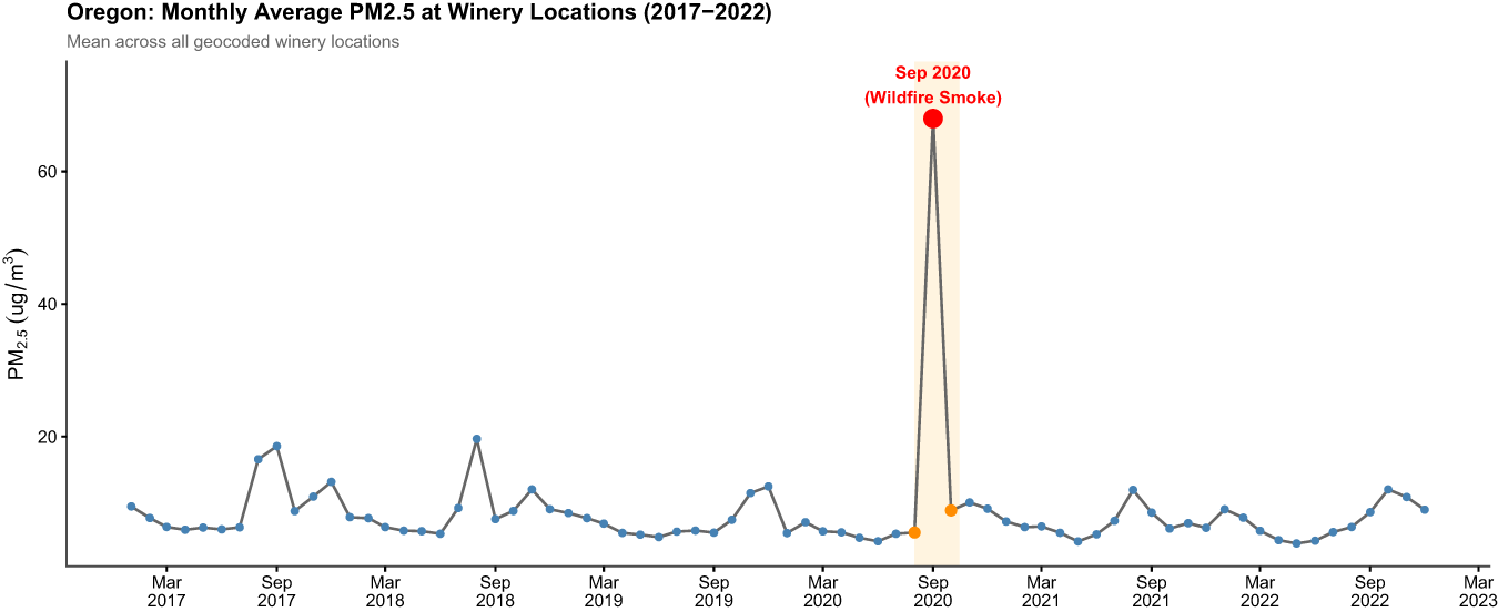
Even though wildfires have been a recurring feature of the West Coast landscape (Liu et al., Reference Liu, Stanturf and Goodrick2010), the 2020 Oregon fire season was unprecedented in its severity. As Figure 2 shows, PM2.5 concentrations at Oregon winery locations spiked dramatically in September 2020, dwarfing levels recorded in any prior year. The timing was especially damaging: grapes are most susceptible to smoke exposure in the weeks immediately before harvest, when absorbed smoke compounds alter the sensory profile of the finished wine in ways that persist through processing (Dungey et al., Reference Dungey, Hayasaka and Wilkinson2011; Tomasino et al., Reference Tomasino, Cerrato, Aragon, Fryer, Garcia, Ashmore and Collins2023). More than 60% of Oregon wineries reported being directly affected by smoke from wildfires, rising to 76% in the Willamette Valley (Oregon Wine Board and Institute for Policy Research & Engagement, 2021).
Monthly mean PM2.5 measurements at Oregon Wineries (2017–2022).

The economic consequences of these events affect wineries through two distinct channels that unfold on very different timescales. The first is a retail market channel: smoke exposure in the pre-harvest period may affect the wines that enter the retail market in subsequent years, impacting sales volumes as smoke-affected vintages reach consumers. The second is a hospitality channel: poor air quality may deter visitors from visiting wine country in the months immediately following a smoke event, directly reducing tasting room revenue and on-site sales. Separating those two channels, and how large and persistent their effects are, motivates our research question.
III. Data
We combine several data sources for this research.
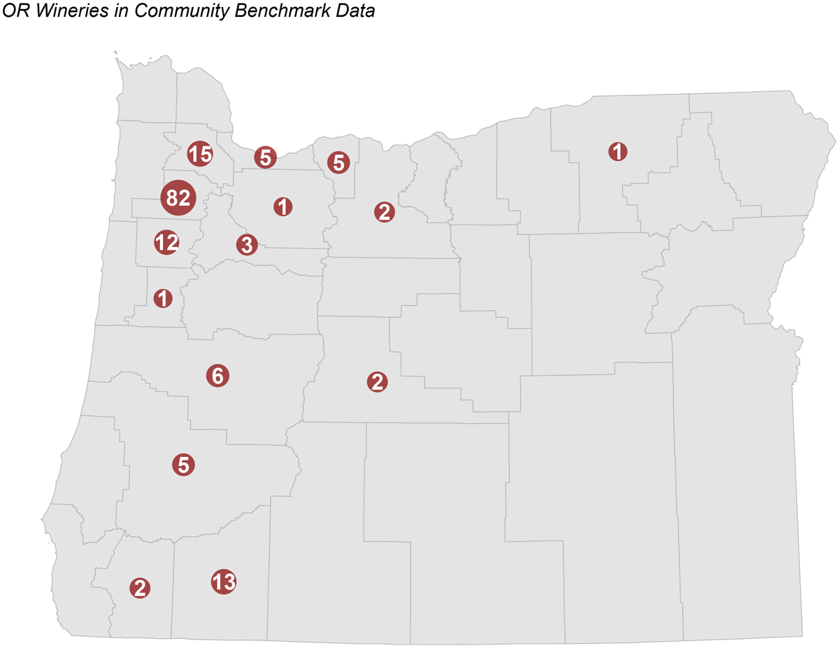
First, we purchased a proprietary dataset that contains visitation and sales data for approximately 160 wineries in Oregon between 2019 and 2024 from Community Benchmark. To protect the identities of those wineries, the names of the wineries are anonymized, and only their zip codes and county names are known to the researchers. This dataset includes key financial performance metrics such as visitation number, tasting room sales, and wine club membership. Figure 3 indicates the approximate locations of wineries for which we have access to this information. We present the full summary of this dataset in Table 1 in the Tables and Figures section.
Map of Oregon winery locations in the Community Benchmark dataset. The number in each circle represents the total number of existing wineries in the dataset.

Summary statistics

Table 1 Long description
Summary statistics are reported as Mean, SD, Min, Max, and N for two panels: Retail Panel and Tasting Room Panel for 2019 to 2024. Panel A lists four retail measures, each with N 3,745: retail sales volume in cases has mean 1,610.193, SD 6,239.530, min 0.100, max 75,186.400; retail price in USD per case has mean 245.923, SD 125.362, min 20.000, max 2,192.000; log retail price has mean 5.414, SD 0.409, min 2.996, max 7.693; September 2020 PM 2.5 in micrograms per cubic meter has mean 68.057, SD 11.513, min 43.493, max 110.936. Panel B lists ten measures with varying N: tasting room sales in USD has mean 45,412.575, SD 57,031.579, min 0.000, max 718,079.000, N 7,021; log tasting room sales has mean 10.162, SD 1.243, min 1.609, max 13.484, N 6,864. Visitors has mean 650.134, SD 888.477, min 0.000, max 14,661.000, N 6,876; log visitors has mean 5.855, SD 1.294, min 0.000, max 9.593, N 6,698. DTC total sales in USD has mean 112,908.455, SD 236,283.912, min 0.000, max 5,937,174.000, N 7,260; log DTC total sales has mean 10.809, SD 1.354, min 3.912, max 15.597, N 7,183. Monthly PM 2.5 raw in micrograms per cubic meter has mean 5.775, SD 5.781, min 1.842, max 177.235, N 11,232; monthly PM 2.5 winsorized p99 has mean 5.596, SD 3.640, min 1.842, max 31.145, N 11,232. Mean temperature in C PRISM has mean 11.282, SD 6.110, min minus 3.726, max 24.597, N 9,920; precipitation in mm PRISM has mean 91.785, SD 80.699, min 0.000, max 412.566, N 9,920.
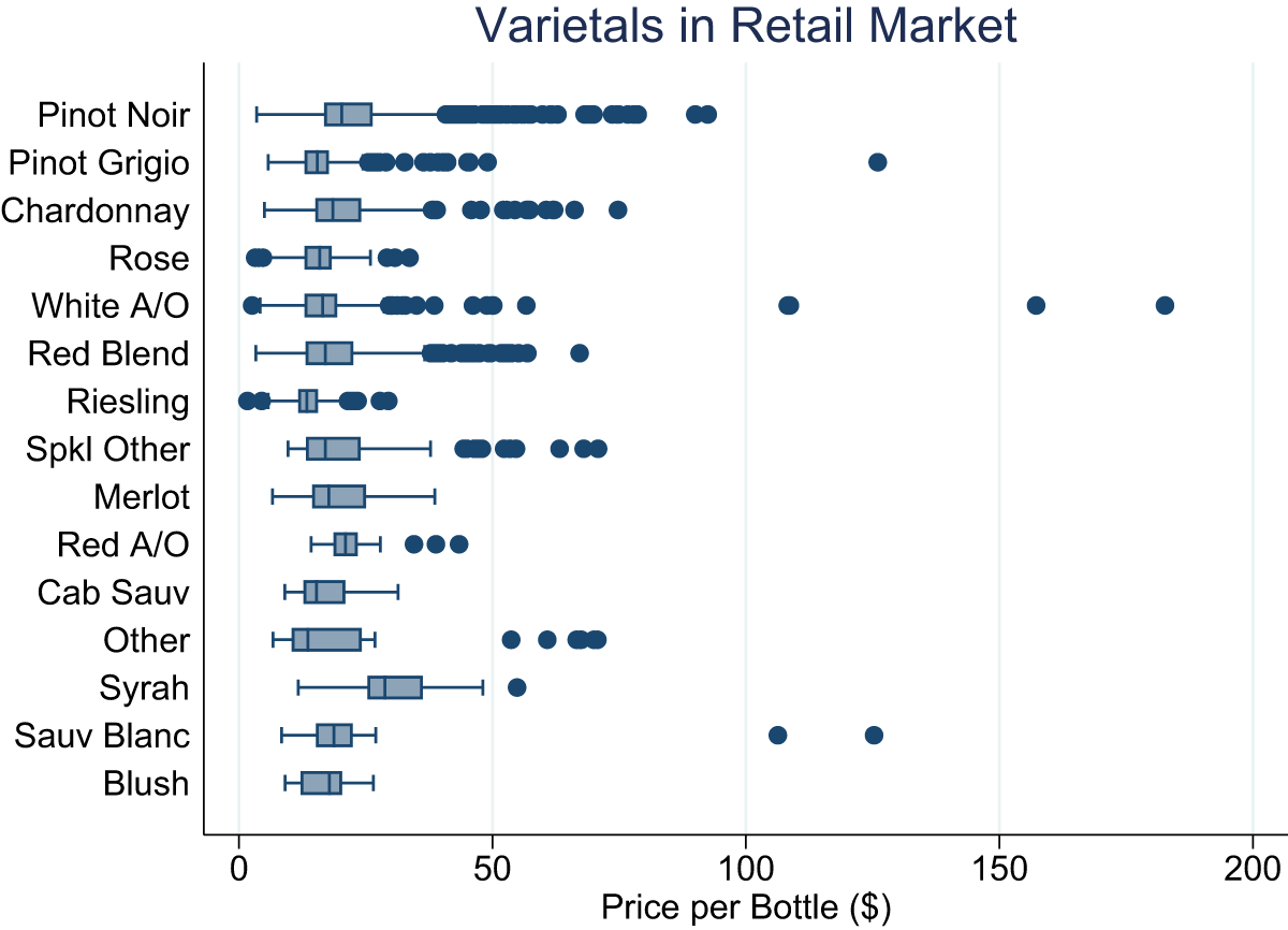
Next, we purchased retail, varietal-specific wine annual sales data between 2018 and 2024 from Gomberg, Fredrikson & Associates.Footnote 3 While this data is coarser and only measures the bottle price and the sales volume of each varietal at the end of each year, this dataset is more representativeFootnote 4 and includes all Oregon wineries that have a presence in the retail market. One limitation of the retail data is that sales volumes are recorded at the brand-varietal-year level without information on the vintage year of wines sold, meaning we cannot directly observe which vintage is driving sales in a given calendar year. Figure 4 details the price range of each varietal in the dataset. In contrast, the data provided by Community Benchmark only includes the clients of the company and is therefore less likely to be representative of the Oregon wine industry. Nevertheless, together, these two datasets allow us to examine the wider impacts of smoke across different consumer populations, from core market participants such as wine club members and tasting room regulars, to more casual wine drinkers reached through the retail channel.
Retail wine sales price by varietal (Source: Retail scanner data).

Figure 4 Long description
Varietals in Retail Market. The horizontal axis is labeled, Price per Bottle (dollar). The range shown is 0 to 200, with tick labels at 0, 50, 100, 150 and 200. The vertical axis lists categories: Pinot Noir, Pinot Grigio, Chardonnay, Rose, White A slash O, Red Blend, Riesling, Spkl Other, Merlot, Red A slash O, Cab Sauv, Other, Syrah, Sauv Blanc, Blush. Each category is shown as a horizontal box and whisker plot with individual points. Pinot Noir: box and whiskers span roughly from about 5 to about 35, with many points extending from about 35 to about 85 and additional points near about 95 and about 125. Pinot Grigio: box and whiskers span roughly from about 5 to about 25, with points extending to about 45 and one point near about 125. Chardonnay: box and whiskers span roughly from about 5 to about 35, with points extending to about 80. Rose: box and whiskers span roughly from about 0 to about 25, with points extending to about 30. White A slash O: box and whiskers span roughly from about 0 to about 30, with points extending to about 60 and isolated points near about 110, about 155 and about 185. Red Blend: box and whiskers span roughly from about 5 to about 35, with many points extending to about 55 and a point near about 70. Riesling: box and whiskers span roughly from about 0 to about 25, with points extending to about 30. Spkl Other: box and whiskers span roughly from about 10 to about 40, with points extending to about 75. Merlot: box and whiskers span roughly from about 10 to about 40. Red A slash O: box and whiskers span roughly from about 15 to about 25, with points near about 35 to about 45. Cab Sauv: box and whiskers span roughly from about 10 to about 30. Other: box and whiskers span roughly from about 10 to about 30, with points near about 55 to about 70. Syrah: box and whiskers span roughly from about 15 to about 55, with a point near about 55. Sauv Blanc: box and whiskers span roughly from about 10 to about 30, with points near about 110 and about 125. Blush: box and whiskers span roughly from about 10 to about 30.
The list of wineries in Oregon, their addresses, and the scale of their operations is provided by Wine Business Analytics. The list includes detailed business information for approximately 850 wineries that are listed as businesses in Oregon. We geocode each winery using its street address and spatially match winery locations to the gridded pollution data using the sf and tidygeocoder packages in R. Figure 1 showcases all wineries in Oregon, and Figure 3 shows county-level locations of wineries for which we have access to monthly metrics.
Additionally, we utilize gridded daily pollution data, specifically GHAP (Global High Air Pollutants). As described in Wei et al. (Reference Wei, Li, Lyapustin, Wang, Dubovik, Schwartz, Sun, Li, Liu and Zhu2023), GHAP is the first dataset of its kind to provide gapless daily PM ${_{2.5}}$ pollution at 1 km resolution at the global level. We use PM
 ${_{2.5}}$ measurements from September 2020 in Oregon to identify the severity of smoke events before the harvesting season. For the tasting room analysis, we assign each winery the mean monthly PM
 ${_{2.5}}$ from the Shen et al. (Reference Shen, Li, Van Donkelaar, Jacobs, Wang and Martin2024) V6GL.03 satellite product, aggregated to the winery's ZIP code. We additionally obtain monthly temperature and precipitation data from PRISM at 4 km resolution (PRISM Climate Group, Oregon State University, 2020), aggregated to the zip code level, and merge these as climate controls with the Community Benchmark dataset.
Combining the data sources described above, we created the following novel datasets. The first is a monthly panel of selected Oregon wineries that measures performance metrics and monthly PM ${_{2.5}}$ levels at the zip code level for the years 2019–2024. The second panel dataset includes annual sales volume and average bottle price alongside the severity of 2020 fires recorded in the GHAP dataset, covering all Oregon wineries present in the retail market for the years 2018–2024. We summarize all datasets in Table 1.
IV. Empirical strategy
a. Retail wine sales
Our primary empirical goal is to estimate how exposure to severe wildfire smoke in the weeks immediately preceding harvest impacts future retail wine sales. We exploit the fact that wildfire activity in the 2020 Oregon fire season varied substantially across space. Some wineries experienced intense late-season smoke events while others, even within the Willamette Valley, did not. This cross-sectional variation in smoke exposure, combined with multiple pre-treatment years (2018–2019) and multiple post-treatment years (2021–2024), forms the basis of our identification strategy.
Rather than collapsing treatment into a binary indicator, we use each winery's mean September PM ${_{2.5}}$ concentration in 2020 as a continuous measure of smoke exposure. Given that the impact of smoke on wine quality is incremental (Jiang et al., Reference Jiang, Bilogrevic, Parker, Francis, Leske, Hayasaka, Barter and Herderich2022; Kennison et al., Reference Kennison, Wilkinson, Pollnitz, Williams and Gibberd2009), this allows us to estimate the dose-response relationship between smoke intensity and sales outcomes while retaining full cross-sectional variation in treatment intensity. We consider the following Two-way Fixed Effects Event Study framework:
 \begin{equation}\text{ln}\left( \text{Volum}{\text{e}_{ivt}} \right) = \sum \limits_{k \neq 2019}{\delta_k}\left( \text{PM2}{\text{5}_i}\times 1\left[ t = k \right] \right)+{\mu_{iv}}+{\gamma_t}+{\varepsilon_{ivt}},\end{equation}
where  $\text{ln}\left( \text{Volum}{\text{e}_{ivt}} \right)$ is the natural log of retail sales volume for brand-varietal
 $iv$ in year
 $t$. The unit of observation is a brand-varietal-year cell, which reflects the structure of the retail scanner data.
 $\text{PM2}{\text{5}_i}$ is the standardized September 2020 mean PM
 ${_{2.5}}$ concentration (in
 $\mu$g/m
 ${^3}$, scaled by a factor of 0.1 from raw GHAP units) at winery
 $i$’s location, extracted from the Global High-resolution PM
 ${_{2.5}}$ (GHAP) satellite product at 1 km resolution. The year indicators
 $1\left[ t = k \right]$ span 2018–2024, with 2019 normalized to zero as the reference year. A one-unit increase in
 $\text{PM2}{\text{5}_i}$ corresponds to a one-standard-deviation increase in winery-level smoke exposure (approximately 11.5
 $\mu$g/m
 ${^3}$), placing all estimates on a comparable scale across specifications.
Our treatment variable is assigned based on each winery's registered business address rather than the location of its vineyards, which may introduce measurement error where the vineyard and the listed business facility locations differ. To the extent this introduces classical measurement error, our estimates are likely attenuated toward zero and should be interpreted as conservative lower bounds; we assess this directly in Section e. While assigning exposure at the AVA level, as in Whitnall and Alston (Reference Whitnall and Alston2025), would reduce this measurement error, it would come at the cost of the within-AVA variation in smoke exposure that underlies our identification strategy.
The coefficients  ${\delta_k}$ estimate the year-by-year impact of smoke events in 2020: values near zero for
 $k \in \left\{ 2018 \right\}$ support the parallel trends assumption, while negative and growing
 ${\delta_k}$ for post-2020 years would indicate persistent smoke-induced sales losses. Brand-varietal fixed effects
 ${\mu_{iv}}$ absorb all time-invariant heterogeneity at the product level, including winery terroir and other winery-specific characteristics. Year fixed effects
 ${\gamma_t}$ absorb macroeconomic shocks on the region common to all wineries. Standard errors are clustered at the winery level. Although the 2020 wildfire season coincided with the COVID-19 pandemic, our identification relies solely on cross-sectional variation in smoke exposure across winery locations rather than on the timing of the 2020 shock. Any COVID impact that affects the entire state is absorbed by year fixed effects.
i. Robustness checks
We report several robustness checks for the retail specification, presented in full in Section VI. Briefly, we re-estimate equation 1 across four alternative specifications varying the fixed effects structure (brand-varietal vs. brand) and clustering level (winery vs. brand). We also examine alternative PM ${_{2.5}}$ treatment measures (September maximum, August–September cumulative) and the assignment of exposure to business addresses.
b. Tasting room and direct-to-consumer sales
Our second analysis examines a distinct economic channel: the direct effect of smoke on winery hospitality operations. Smoky conditions can deter visitors from traveling to wine country, reducing foot traffic at tasting rooms and suppressing on-site and direct-to-consumer (DTC) sales independently of any vintage quality effects. To study this mechanism, we use monthly winery-level data from the Community Benchmark panel, which tracks tasting room revenue, visitor counts, and DTC sales for 158 Oregon wineries from January 2019 through December 2024. This analysis captures the impacts of smoke events throughout the six-year period and adds robustness to our analysis.
Because the tasting room wineries are anonymized, we cannot match them to winery-level GHAP coordinates as in the retail analysis. Instead, we assign each winery the mean monthly PM ${_{2.5}}$ from the Shen et al. (Reference Shen, Li, Van Donkelaar, Jacobs, Wang and Martin2024) V6GL.03 satellite product, aggregated to the winery's ZIP code. We estimate the following specification:
 \begin{equation}\text{ln}\left( {Y_{it}} \right) = \beta \text{}\text{PM2}{\text{5}_{z,t-1}}+{\alpha_i}+{\delta_t}+{\varepsilon_{it}},\end{equation}
where  ${Y_{it}}$ is the outcome for winery
 $i$ in month
 $t$ (tasting room sales, visitor counts, or DTC total sales),
 $\text{PM2}{\text{5}_{z,t-1}}$ is the standardized mean PM
 ${_{2.5}}$ in ZIP code
 $z$ in the previous month,
 ${\alpha_i}$ are winery fixed effects that absorb all time-invariant winery heterogeneity, and
 ${\delta_t}$ are month-by-year fixed effects that absorb aggregate seasonal and macroeconomic shocks. Standard errors are clustered at the winery level. We winsorize PM
 ${_{2.5}}$ at the 99th percentile prior to standardization to limit the influence of extreme outlier observations in ZIP codes directly adjacent to fire zones.
The one-month lag specification reflects the primary channel through which smoke affects tasting room business: prospective visitors who observe or anticipate smoky conditions in a given month cancel or reschedule planned visits, with the effect materializing in the following month's revenue and foot traffic. This timing is consistent with typical booking horizons for wine country visits, where reservations are commonly made days to weeks in advance. We verify this timing interpretation by also estimating a specification that includes the contemporaneous PM ${_{2.5}}$ alongside the lag; the contemporaneous coefficient is uniformly small and statistically indistinguishable from zero across all outcomes, while the lagged coefficient is unchanged, supporting the lag-only specification as the preferred estimating equation.
While the COVID-19 pandemic also disrupted tasting room operations in our study period, month-by-year fixed effects absorb all aggregate shocks common to the sample. Winery fixed effects absorb time-invariant differences across wineries but not differential timing, so we cannot rule out that wineries in higher-smoke ZIP codes resumed normal operations on a different schedule. We address this partially by re-estimating on the 2022 sample alone.
V. Results
a. Retail wine sales
i. Sales volume
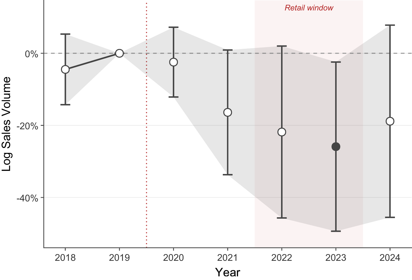
Figure 5 presents the pooled event study estimates from equation 1. The pre-treatment coefficient for 2018 is small and statistically indistinguishable from zero ( ${\hat{\delta}_{2018}} = -0.045$, p = 0.37), providing no evidence of differential pre-existing trends across wineries with different levels of smoke exposure. Following the smoke shock, the estimated coefficients are negative in every post-treatment year and grow in magnitude through 2023, though only the 2023 estimate is significant at the 5% level. The point estimates move from
 ${\hat{\delta}_{2021}} = -0.164$ (
 $p = 0.063$) to
 ${\hat{\delta}_{2022}} = -0.218$ (
 $p = 0.072$) and
 ${\hat{\delta}_{2023}} = -0.259$ (
 $p = 0.031$), corresponding to sales losses of approximately 15%, 20%, and 23%, respectively relative to the 2019 baseline. The effect attenuates in 2024 (
 ${\hat{\delta}_{2024}} = -0.188$,
 $p = 0.165$), suggesting the shock is largely, though not fully, absorbed by the end of the sample period. This pattern is consistent with the 2020 harvest entering the retail market with a two-to-three-year lag, with the peak effect observed in 2023 when 2020 vintage wines are likely to be more prominent on retail shelves.
Effect of wildfire smoke on retail wine sales: all varietals. Coefficients  ${\hat{\delta}_k}$ from equation 1, all varietals pooled. Treatment variable is September 2020 mean PM
 ${_{2.5}}$ (standardized; 1 SD
 $\approx$ 11.6
 $\mu$g/m
 ${^3}$). Filled circles indicate
 $p \lt 0.05$; hollow circles indicate
 $p \ge 0.05$. Shaded band = 95% confidence interval. Reference year is 2019. Shaded region denotes the primary retail window (2022–23). Brand-varietal and year fixed effects; standard errors clustered at the winery level.

To economically motivate the magnitude, a one-standard-deviation difference in September PM ${_{2.5}}$ exposure corresponds to approximately 11.6
 $\mu$g/m
 ${^3}$ of smoke particulates in the air. The difference in exposure between the median and 75th percentile wineries corresponds to a retail sales loss of approximately 14% in 2023.
ii. Heterogeneity by varietal
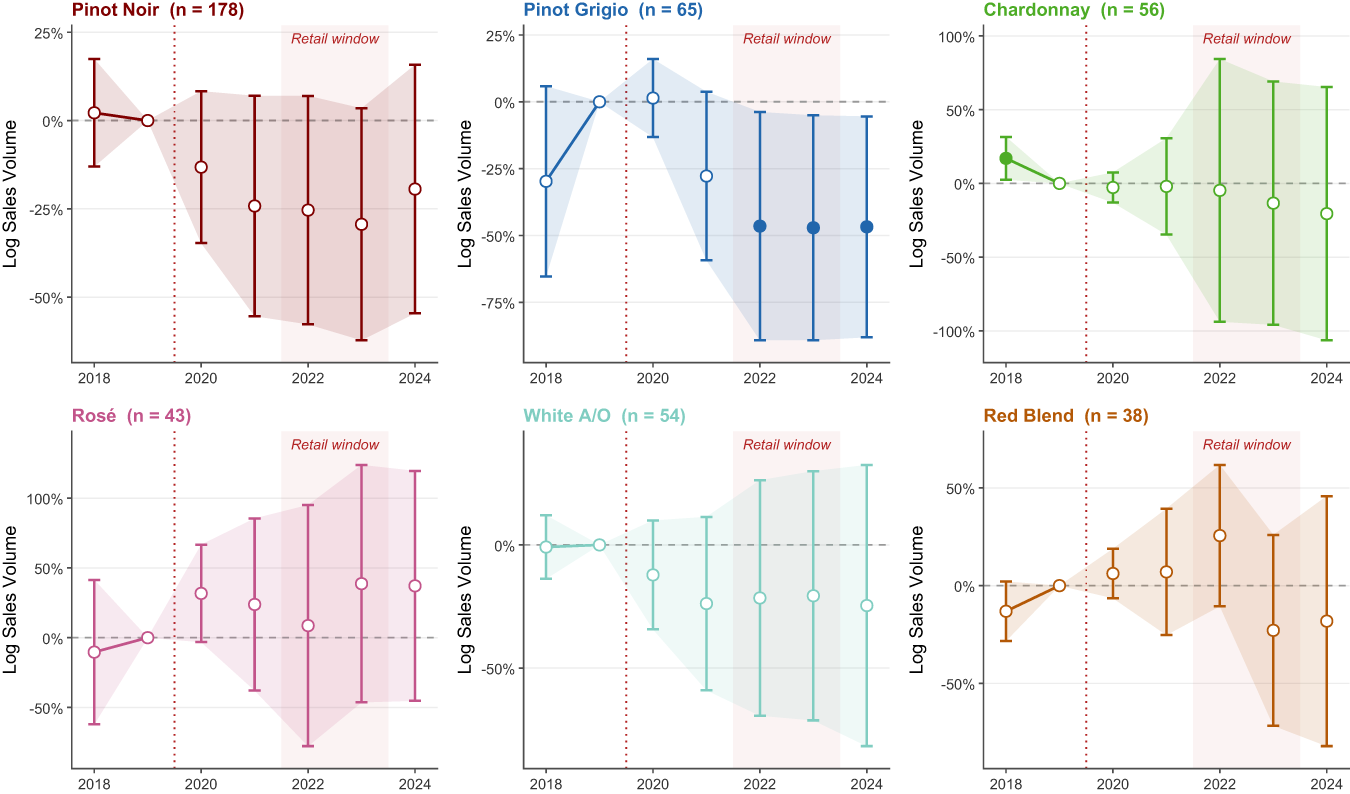
Figure 6 further disaggregates the pooled result by varietal. The effects are far from uniform across the six varietals we examine, and the heterogeneity has a clear economic interpretation.
Effect of wildfire smoke on retail wine sales: By varietal. Each panel re-estimates equation 1 on the relevant varietal subsample.  $n$ denotes the number of brand-varietal units. Filled circles indicate
 $p \lt 0.05$; hollow circles indicate
 $p \ge 0.05$. Shaded band = 95% confidence interval. Reference year is 2019. Chardonnay exhibits a significant pre-trend coefficient in 2018 and post-period estimates for this varietal should be interpreted with caution. Brand-varietal and year fixed effects; standard errors clustered at the winery level.

Figure 6 Long description
Six line graphs titled Pinot Noir, Pinot Grigio, Chardonnay, Rose, White A slash O and Red Blend, each with n shown in parentheses. Common axes and markings across all six graphs: The horizontal axis shows years 2018, 2020, 2022 and 2024. The vertical axis label is Log Sales Volume. Each graph includes a horizontal dashed line at 0 percent and a vertical dotted line at 2019. Each graph includes the text, Retail window, over a shaded vertical band spanning the later years. Pinot Noir, n equals 178: Vertical axis tick labels are 25 percent, 0 percent, negative 25 percent and negative 50 percent. Plotted points are shown for 2018 through 2024 with vertical error bars and a shaded band. The point at 2018 is slightly above 0 percent. The point at 2019 is at about 0 percent. The point at 2020 is below 0 percent. The points for 2021, 2022 and 2023 are below 0 percent, near the negative 25 percent line. The point at 2024 is below 0 percent. Pinot Grigio, n equals 65: Vertical axis tick labels are 25 percent, 0 percent, negative 25 percent, negative 50 percent and negative 75 percent. Plotted points are shown for 2018 through 2024 with vertical error bars and a shaded band. The point at 2018 is below 0 percent, near negative 25 percent. The point at 2019 is at about 0 percent. The point at 2020 is slightly above 0 percent. The point at 2021 is below 0 percent, near negative 25 percent. The points for 2022, 2023 and 2024 are below 0 percent, near negative 50 percent. Chardonnay, n equals 56: Vertical axis tick labels are 100 percent, 50 percent, 0 percent, negative 50 percent and negative 100 percent. Plotted points are shown for 2018 through 2024 with vertical error bars and a shaded band. The point at 2018 is above 0 percent. The point at 2019 is at about 0 percent. The points at 2020 and 2021 are near 0 percent. The points at 2022, 2023 and 2024 are below 0 percent. Rose, n equals 43: Vertical axis tick labels are 100 percent, 50 percent, 0 percent and negative 50 percent. Plotted points are shown for 2018 through 2024 with vertical error bars and a shaded band. The point at 2018 is below 0 percent. The point at 2019 is at about 0 percent. The points at 2020 and 2021 are above 0 percent. The point at 2022 is above 0 percent. The points at 2023 and 2024 are above 0 percent. White A slash O, n equals 54: Vertical axis tick labels are 0 percent and negative 50 percent. Plotted points are shown for 2018 through 2024 with vertical error bars and a shaded band. The point at 2018 is near 0 percent. The point at 2019 is near 0 percent. The point at 2020 is below 0 percent. The points at 2021, 2022, 2023 and 2024 are below 0 percent. Red Blend, n equals 38: Vertical axis tick labels are 50 percent, 0 percent and negative 50 percent. Plotted points are shown for 2018 through 2024 with vertical error bars and a shaded band. The point at 2018 is below 0 percent. The point at 2019 is at about 0 percent. The points at 2020 and 2021 are above 0 percent. The point at 2022 is above 0 percent. The points at 2023 and 2024 are below 0 percent.
Pinot Grigio is the most strongly and consistently affected varietal. Estimated sales losses grow from  $-$24% in 2021 to
 $-$37% to
 $-$38% in 2022–2024, with all post-treatment coefficients statistically significant at least at the 10% level (and 5% level from 2022 onward). The 2018 pre-trend coefficient for Pinot Grigio is marginally significant at the 10% level, which warrants some caution in interpreting the post-treatment estimates. Notably however, the pre-trend is positive while the post-treatment effects are negative and growing in magnitude.
Pinot Noir, which accounts for approximately 49% of retail sales in our sample, shows a consistently negative trajectory throughout 2021–2023, with estimated losses of approximately 21%–25%. The 2023 coefficient ( ${\hat{\delta}_{2023}} = -0.294$) is statistically significant at the 10% level (
 $p = 0.077$). While the significance is marginal, the directional consistency across all posttreatment years and the economic magnitude are notable. Together, Pinot Noir and Pinot Grigio account for approximately 75% of total retail volume in the sample, and a back-of-the-envelope decomposition confirms that their combined contribution accounts for nearly all of the pooled
 $-$23% effect: Pinot Noir contributes roughly 12 percentage points (49% share
 $\times$
 $-$25% effect) and Pinot Grigio roughly 9 percentage points (26% share
 $\times$
 $-$35% effect).
Chardonnay exhibits a large and significant pre-trend coefficient ( ${\hat{\delta}_{2018}} = -0.297$,
 $p = 0.093$), indicating that treated and control Chardonnay producers were on divergent trajectories before the 2020 fires. Unlike Pinot Grigio, where the pre-trend runs opposite to the posttreatment effects, the Chardonnay pre-trend runs in the same direction as the post-period estimates, meaning we cannot rule out that the posttreatment decline reflects a continuation of preexisting trends rather than a smoke effect. We therefore exclude Chardonnay from our headline conclusions, though we retain it in Figure 6 for completeness and note that the post-period estimates should be interpreted with caution.
Rosé, White A/OFootnote 5, and Red Blend show no statistically significant post-treatment effects in either direction, with coefficients close to zero and wide confidence intervals throughout the post-treatment period. The absence of significant effects for these varietals is consistent with their more limited regional identity in the Oregon market. Unlike Pinot Noir and Pinot Grigio, these varietals have not carried a strong Oregon appellation branding and may therefore face less reputational exposure from a smoke event. Table 2 presents the full results.
Effect of wildfire smoke on retail wine sales volume

Table 2 Long description
Coefficients and clustered standard errors are reported for interaction terms by year relative to 2019, with columns for All varietals, Pinot Noir, Pinot Grigio, Chardonnay, Rose, White A O, and Red Blend. For delta 2018, coefficients are minus 0.045 for All varietals, 0.022 for Pinot Noir, minus 0.297 with one star for Pinot Grigio, 0.170 with two stars for Chardonnay, minus 0.104 for Rose, minus 0.009 for White A O, and minus 0.131 with one star for Red Blend, with standard errors 0.050, 0.077, 0.177, 0.072, 0.256, 0.064, and 0.075. For delta 2021, coefficients are minus 0.164 with one star, minus 0.242, minus 0.278 with one star, minus 0.020, 0.238, minus 0.238, and 0.070, with standard errors 0.088, 0.158, 0.157, 0.162, 0.304, 0.175, and 0.159. For delta 2022, coefficients are minus 0.218 with one star, minus 0.254, minus 0.465 with two stars, minus 0.047, 0.086, minus 0.215, and 0.256, with standard errors 0.121, 0.164, 0.213, 0.443, 0.427, 0.238, and 0.178. For delta 2023, coefficients are minus 0.259 with two stars, minus 0.294 with one star, minus 0.471 with two stars, minus 0.134, 0.387, minus 0.207, and minus 0.229, with standard errors 0.119, 0.166, 0.210, 0.410, 0.420, 0.252, and 0.240. For delta 2024, coefficients are minus 0.188, minus 0.194, minus 0.468 with two stars, minus 0.205, 0.371, minus 0.246, and minus 0.182, with standard errors 0.135, 0.178, 0.206, 0.427, 0.407, 0.284, and 0.315. Observations are 3745 for All varietals, 1246 for Pinot Noir, 455 for Pinot Grigio, 392 for Chardonnay, 301 for Rose, 378 for White A O, and 266 for Red Blend, and both Brand varietal FE and Year FE are Yes in every column.
Note: Dependent variable is log retail sales volume. Treatment is September 2020 mean PM ${_{2.5}}$ (standardized; 1 SD = 11.6
 $\mu$g/m
 ${^3}$). Standard errors clustered at the winery level in parentheses.
 ${\delta_k}$ = interaction coefficient for year
 $k$ relative to 2019. *
 $p \lt 0.10$, **
 $p \lt 0.05$, ***
 $p \lt 0.01$.
iii. Price effects
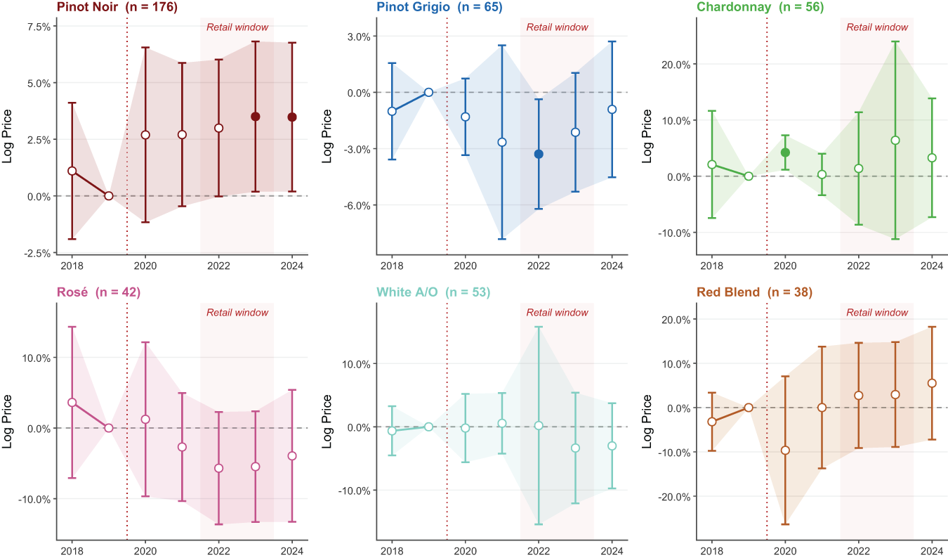
Table 3 and Figure 7 report the corresponding estimates from equation 1 with log retail price as the outcome. The pooled price effect is negligible and statistically indistinguishable from zero across all post-treatment years. Separating impacts by varietal, however, reveals heterogeneity in price responses.
Effect of wildfire smoke on retail wine prices

Table 3 Long description
Interaction coefficients by year relative to 2019 are reported for log retail price per unit across seven columns: All varietals, Pinot Noir, Pinot Grigio, Chardonnay, Rose, White A O, and Red Blend, with standard errors in parentheses. For delta 2018, coefficients are minus 0.003 for All varietals, 0.011 for Pinot Noir, minus 0.010 for Pinot Grigio, 0.021 for Chardonnay, 0.036 for Rose, minus 0.006 for White A O, and minus 0.032 for Red Blend. For delta 2021, coefficients are 0.003 for All varietals, 0.027 with one star for Pinot Noir, minus 0.027 for Pinot Grigio, 0.003 for Chardonnay, minus 0.027 for Rose, 0.006 for White A O, and 0.000 for Red Blend. For delta 2022, coefficients are minus 0.002 for All varietals, 0.030 with one star for Pinot Noir, minus 0.033 with two stars for Pinot Grigio, 0.014 for Chardonnay, minus 0.057 for Rose, 0.002 for White A O, and 0.027 for Red Blend. For delta 2023, coefficients are 0.003 for All varietals, 0.035 with two stars for Pinot Noir, minus 0.021 for Pinot Grigio, 0.064 for Chardonnay, minus 0.055 for Rose, minus 0.034 for White A O, and 0.029 for Red Blend. For 2024, coefficients are 0.011 for All varietals, 0.035 with two stars for Pinot Noir, minus 0.009 for Pinot Grigio, 0.033 for Chardonnay, minus 0.039 for Rose, minus 0.030 for White A O, and 0.055 for Red Blend. Observations are 2541 for All varietals, 861 for Pinot Noir, 392 for Pinot Grigio, 239 for Chardonnay, 200 for Rose, 237 for White A O, and 161 for Red Blend, and both Brand varietal FE and Year FE are Yes in every column.
Note: Dependent variable is log retail price per unit. Treatment is the September 2020 mean PM ${_{2.5}}$ (standardized; 1 SD = 11.6
 $\mu$g/m
 ${^3}$). Standard errors clustered at the winery level in parentheses.
 ${\delta_k}$ = interaction coefficient for year
 $k$ relative to 2019. *
 $p \lt 0.10$, **
 $p \lt 0.05$, ***
 $p \lt 0.01$.
Effect of wildfire smoke on retail wine prices: By varietal. Each panel re-estimates equation 1 with log retail price as the outcome on the relevant varietal subsample.  $n$ denotes the number of brand-varietal units. Filled circles indicate
 $p \lt 0.05$; hollow circles indicate
 $p \ge 0.05$. Shaded band = 95% confidence interval. Reference year is 2019. Brand-varietal and year fixed effects; standard errors clustered at the winery level.

Figure 7 Long description
A showing Pinot Noir, n equals 176. The horizontal axis is labeled 2018, 2020, 2022, 2024. The vertical axis is labeled Log Price, with tick labels minus 2.5, 0.0, 2.5, 5.0, 7.5. Text inside the plot reads, Retail window. A vertical dotted line is at 2020. A horizontal dashed line is at 0.0. Circular markers are connected by a line. Each marker has a vertical error bar. A shaded band surrounds the line. Data points as coordinate pairs: (2018, 1.0), (2019, 0.0), (2020, 2.5), (2021, 2.5), (2022, 3.0), (2023, 3.5), (2024, 3.5). B showing Pinot Grigio, n equals 65. The horizontal axis is labeled 2018, 2020, 2022, 2024. The vertical axis is labeled Log Price, with tick labels minus 6.0, minus 3.0, 0.0, 3.0. Text inside the plot reads, Retail window. A vertical dotted line is at 2020. A horizontal dashed line is at 0.0. Circular markers are connected by a line. Each marker has a vertical error bar. A shaded band surrounds the line. Data points as coordinate pairs: (2018, minus 1.0), (2019, 0.0), (2020, minus 1.5), (2021, minus 2.5), (2022, minus 3.0), (2023, minus 2.0), (2024, minus 1.0). C showing Chardonnay, n equals 56. The horizontal axis is labeled 2018, 2020, 2022, 2024. The vertical axis is labeled Log Price, with tick labels minus 10.0, 0.0, 10.0, 20.0. Text inside the plot reads, Retail window. A vertical dotted line is at 2020. A horizontal dashed line is at 0.0. Circular markers are connected by a line. Each marker has a vertical error bar. A shaded band surrounds the line. Data points as coordinate pairs: (2018, 2.0), (2019, 0.0), (2020, 4.0), (2021, 0.0), (2022, 1.0), (2023, 6.0), (2024, 3.0). D showing Rose, n equals 42. The horizontal axis is labeled 2018, 2020, 2022, 2024. The vertical axis is labeled Log Price, with tick labels minus 10.0, 0.0, 10.0. Text inside the plot reads, Retail window. A vertical dotted line is at 2020. A horizontal dashed line is at 0.0. Circular markers are connected by a line. Each marker has a vertical error bar. A shaded band surrounds the line. Data points as coordinate pairs: (2018, 4.0), (2019, 0.0), (2020, 1.0), (2021, minus 3.0), (2022, minus 6.0), (2023, minus 6.0), (2024, minus 4.0). E showing White A/O, n equals 53. The horizontal axis is labeled 2018, 2020, 2022, 2024. The vertical axis is labeled Log Price, with tick labels minus 10.0, 0.0, 10.0. Text inside the plot reads, Retail window. A vertical dotted line is at 2020. A horizontal dashed line is at 0.0. Circular markers are connected by a line. Each marker has a vertical error bar. A shaded band surrounds the line. Data points as coordinate pairs: (2018, minus 1.0), (2019, 0.0), (2020, 0.0), (2021, 0.0), (2022, 0.0), (2023, minus 3.0), (2024, minus 3.0). F showing Red Blend, n equals 38. The horizontal axis is labeled 2018, 2020, 2022, 2024. The vertical axis is labeled Log Price, with tick labels minus 20.0, minus 10.0, 0.0, 10.0, 20.0. Text inside the plot reads, Retail window. A vertical dotted line is at 2020. A horizontal dashed line is at 0.0. Circular markers are connected by a line. Each marker has a vertical error bar. A shaded band surrounds the line. Data points as coordinate pairs: (2018, minus 3.0), (2019, 0.0), (2020, minus 10.0), (2021, 0.0), (2022, 3.0), (2023, 3.0), (2024, 6.0).
Pinot Grigio exhibits declining prices alongside declining volumes. The 2022 price coefficient ( ${\hat{\delta}_{2022}} = -0.033$,
 $p = 0.028$) indicates a 3.2% price reduction relative to control wineries, with both price and quantity moving in the same direction.
Pinot Noir, by contrast, shows rising prices post-2020, with coefficients of approximately  $+$2.7% to
 $+$3.6% throughout 2021–2024, significant at the 5%–10% level. We briefly discuss these contrasting price responses across varietals in Section VII.
b. Tasting room and direct-to-consumer sales
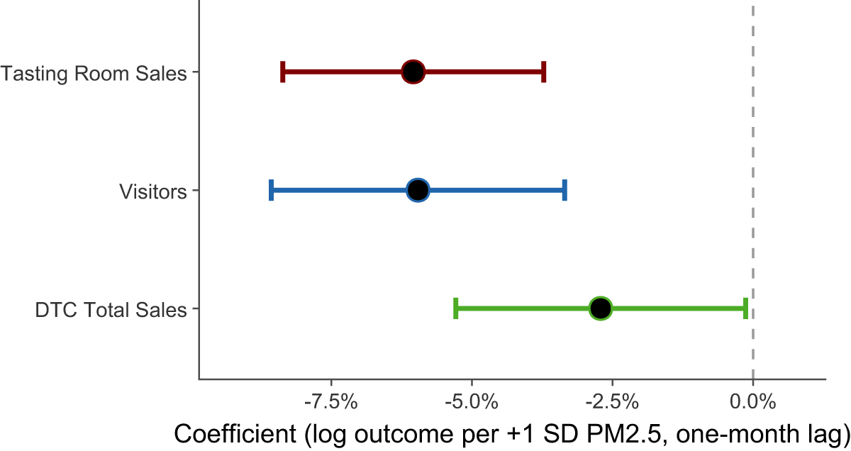
Figure 8 presents the main results from equation 2 under our preferred specification (PM ${_{2.5}}$ winsorized at the 99th percentile, standard errors clustered at the winery level). A one-standard-deviation increase in lagged ZIP-code PM
 ${_{2.5}}$ is associated with a 5.8% decline in tasting room sales (
 $p \lt 0.01$), a 5.8% decline in visitor counts (
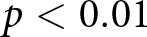 $p \lt 0.01$), and a 2.7% decline in DTC total sales (
 $p \lt 0.05$). The effect is statistically significant and economically meaningful across all three outcomes; the somewhat smaller magnitude for DTC sales is consistent with the nature of that channel, since online and phone orders are less sensitive to local air quality than in-person visits.
Effect of wildfire smoke on tasting room operations. Coefficients  $\hat{\beta}$ from equation 2 under the preferred specification (PM
 ${_{2.5}}$ winsorized at the 99th percentile; 1 SD
 $\approx$ 3.6
 $\mu$g/m
 ${^3}$ after winsorizing). Filled circles indicate
 $p \lt 0.05$; hollow circles indicate
 $p \ge 0.05$. Horizontal bars denote 95% confidence intervals. Winery and month-by-year fixed effects; standard errors clustered at the winery level.
 $N = 158$ wineries.

The timing of the effect is informative about the underlying mechanism. Smoke in month  $t$ reduces visits and sales in month
 $t+1$, consistent with a booking and cancellation channel: prospective visitors who observe smoky conditions cancel or reschedule planned trips, with the impact registering in the following month's revenue. The contemporaneous coefficient is uniformly small and statistically indistinguishable from zero across all three outcomes, ruling out a purely same-month air quality channel as the primary driver.Footnote 6
These estimates should be interpreted as conservative lower bounds on the true effect. The tasting room wineries are anonymized and can only be located to the ZIP code level, so the PM treatment variable is aggregated from winery-level to ZIP-code-level. This geographic aggregation introduces classical measurement error that attenuates our estimates toward zero. The true winery-level effect is likely larger in magnitude than what we estimate here.
The tasting room findings complement the retail results in an informative way. The retail analysis captures the reduced-form effect of smoke exposure on market quantities and prices in the retail market, with results suggesting that there is a several-year lag between smoke events and their impacts on retail sales. The tasting room analysis captures a simpler mechanism, with smoky conditions directly discouraging in-person visits to wineries regardless of vintage quality. Together they document two economically distinct channels through which wildfire smoke affects Oregon wineries: retail market outcomes in subsequent years, and hospitality revenue in the months immediately following a smoke exposure.
i. Robustness
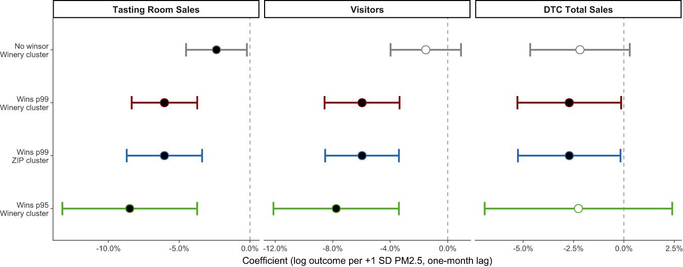
Figure 9 in Section VI reports the tasting room estimates across four alternative specifications varying the winsorizing threshold and clustering level. The negative effect on tasting room sales and visitors is consistent across all specifications, with significance strengthening under the p99 winsorizing specifications. The raw (unwinsorized) estimates are attenuated toward zero, reflecting the influence of extreme PM outliers in ZIP codes adjacent to fire zones; visitor counts in particular lose significance without winsorizing. The p99 winsorized result is therefore our preferred specification.
Tasting room results: robustness to winsorizing and clustering. Each panel shows  $\hat{\beta}$ from equation 2 for the indicated outcome across four specifications. Filled circles indicate
 $p \lt 0.05$; hollow circles indicate
 $p \ge 0.05$. Horizontal bars denote 95% confidence intervals. Winery and month-by-year fixed effects. ZIP cluster
 $n = 53$; winery cluster
 $n = 158$.

Figure 9 Long description
Tasting Room Sales. The x-axis is labeled, Coefficient, open parenthesis log outcome per plus 1 standard deviation PM2.5, one month lag close parenthesis. The x-axis shows tick labels at minus 10.0 percent, minus 5.0 percent and 0.0 percent. Four horizontal confidence intervals with point markers are shown at the y-axis categories, No winsor, Winery cluster; Wins p99, Winery cluster; Wins p99, ZIP cluster; Wins p95, Winery cluster. The point markers are positioned between minus 10.0 percent and 0.0 percent, with the right ends of the intervals near 0.0 percent. Visitors. The x-axis is labeled, Coefficient, open parenthesis log outcome per plus 1 standard deviation PM2.5, one month lag close parenthesis. The x-axis shows tick labels at minus 12.0 percent, minus 8.0 percent, minus 4.0 percent and 0.0 percent. Four horizontal confidence intervals with point markers are shown at the y-axis categories, No winsor, Winery cluster; Wins p99, Winery cluster; Wins p99, ZIP cluster; Wins p95, Winery cluster. The point markers are positioned between minus 12.0 percent and 0.0 percent, with the right ends of the intervals near 0.0 percent. DTC Total Sales. The x-axis is labeled, Coefficient, open parenthesis log outcome per plus 1 standard deviation PM2.5, one month lag close parenthesis. The x-axis shows tick labels at minus 5.0 percent, minus 2.5 percent, 0.0 percent and 2.5 percent. Four horizontal confidence intervals with point markers are shown at the y-axis categories, No winsor, Winery cluster; Wins p99, Winery cluster; Wins p99, ZIP cluster; Wins p95, Winery cluster. The point markers are positioned between minus 5.0 percent and 0.0 percent, with one interval extending to the right of 0.0 percent toward 2.5 percent.
As a further check, we re-estimate equation 2 restricting the sample to 2022, a year in which Oregon's COVID-related restrictions had been fully lifted. Point estimates remain negative across all three outcomes and are comparable in magnitude to the full-sample results, though precision is reduced given the substantially smaller sample. We also note that lingering COVID-related changes in visitor behavior may have compounded the smoke deterrent effect in the full sample.
VI. Robustness checks
a. Alternative fixed effects and clustering: retail
Table 4 reports the pooled event study estimates across four alternative specifications that vary the fixed effects structure and clustering level. Columns (1) and (2) use brand-varietal fixed effects with winery and brand clustering, respectively; columns (3) and (4) replace brand-varietal with brand fixed effects under the same two clustering choices. Across all four columns, point estimates are identical to three decimal places. Standard errors are marginally wider under brand-level clustering, reflecting the unbalanced cluster structure that arises because 78% of brands in our sample consist of a single winery, a pattern that favors winery-level clustering as the preferred choice. The pre-trend coefficient remains small and insignificant throughout. The pooled result is significant at the 5% level in 2023 across all specifications, and at the 10% level in 2021 and 2022 in all four columns.
Robustness: FE and clustering—all varietals

Table 4 Long description
Regression coefficients are reported for delta 2018, delta 2021, delta 2022, delta 2023, and delta 2024 across four columns: BV FE Winery cluster, BV FE Brand cluster, Brand FE Winery cluster, and Brand FE Brand cluster. For delta 2018, the coefficient is minus 0.045 in all four columns, with standard errors 0.050, 0.049, 0.050, and 0.049. For delta 2021, the coefficient is minus 0.164 in all four columns, with a single star in the two Winery cluster columns and two stars in the two Brand cluster columns; standard errors are 0.088, 0.080, 0.088, and 0.080. For delta 2022, the coefficient is minus 0.218 with one star in all four columns; standard errors are 0.121, 0.124, 0.121, and 0.124. For delta 2023, the coefficient is minus 0.259 with two stars in all four columns; standard errors are 0.119, 0.124, 0.119, and 0.124. For delta 2024, the coefficient is minus 0.188 in all four columns with no stars; standard errors are 0.135, 0.143, 0.135, and 0.143. Observations are 3745 in every column; brand varietal fixed effects are Yes in the two BV FE columns and No in the two Brand FE columns, while brand fixed effects are No in the BV FE columns and Yes in the Brand FE columns; year fixed effects are Yes in all columns; cluster level is Winery for the first and third columns and Brand for the second and fourth columns.
Note: Dependent variable is log retail sales volume. Treatment is the September 2020 mean PM ${_{2.5}}$ (standardized; 1 SD = 11.6
 $\mu$g/m
 ${^3}$). Columns differ in fixed effects and clustering choice. BV FE = brand-varietal fixed effects; Brand FE = brand fixed effects. Standard errors in parentheses. *
 $p \lt 0.10$, **
 $p \lt 0.05$, ***
 $p \lt 0.01$.
Tables 5 and 6 replicate this exercise for Pinot Noir and Pinot Grigio, respectively. For Pinot Noir, the 2023 coefficient is significant at the 10% level under winery clustering but falls just short of this threshold under brand clustering, consistent with the cluster structure discussion above. For Pinot Grigio, the 2022–2024 coefficients are significant at the 5% level across all four specifications, reinforcing the robustness of this finding.
Robustness: FE and clustering—Pinot Noir

Table 5 Long description
Regression coefficients are reported for delta 2018, delta 2021, delta 2022, delta 2023, and delta 2024 across four columns: BV FE Winery cluster, BV FE Brand cluster, Brand FE Winery cluster, and Brand FE Brand cluster. Delta 2018 is 0.022 in all columns, with standard errors 0.077 for winery clustering and 0.084 for brand clustering. Delta 2021 is minus 0.242 in all columns, with standard errors 0.158 for winery clustering and 0.156 for brand clustering. Delta 2022 is minus 0.254 in all columns, with standard errors 0.164 for winery clustering and 0.174 for brand clustering. Delta 2023 is minus 0.294 in all columns, with a star in the two winery cluster columns and no star in the two brand cluster columns; standard errors are 0.166 for winery clustering and 0.184 for brand clustering. Delta 2024 is minus 0.194 in all columns, with standard errors 0.178 for winery clustering and 0.193 for brand clustering. Observations are 1246 in every column; brand varietal fixed effects are Yes only in the two BV FE columns, brand fixed effects are Yes only in the two Brand FE columns, year fixed effects are Yes in all columns, and the cluster level is Winery for the first and third columns and Brand for the second and fourth columns.
Note: Dependent variable is log retail sales volume. Treatment is September 2020 mean PM ${_{2.5}}$ (standardized; 1 SD = 11.6
 $\mu$g/m
 ${^3}$). Columns differ in fixed effects and clustering choice. BV FE = brand-varietal fixed effects; Brand FE = brand fixed effects. Standard errors in parentheses. *
 $p \lt 0.10$, **
 $p \lt 0.05$, ***
 $p \lt 0.01$.
Robustness: FE and clustering—Pinot Grigio

Table 6 Long description
Regression coefficients are reported for year indicators labeled delta 2018, delta 2021, delta 2022, delta 2023, and delta 2024 across four specifications: BV FE Winery cluster, BV FE Brand cluster, Brand FE Winery cluster, and Brand FE Brand cluster. For delta 2018, the coefficient is minus 0.297 with a star in the two Winery cluster columns and minus 0.297 without a star in the two Brand cluster columns; standard errors are 0.177 for Winery cluster and 0.179 for Brand cluster. For delta 2021, the coefficient is minus 0.278 with a star in all four columns; standard errors are 0.157 for Winery cluster and 0.160 for Brand cluster. For delta 2022, delta 2023, and delta 2024, coefficients are minus 0.465, minus 0.471, and minus 0.468, each with two stars in all four columns; standard errors are 0.213 and 0.212 for delta 2022, 0.210 for delta 2023, and 0.206 for delta 2024. Observations are 455 in every column. Fixed effects rows indicate brand varietal fixed effects are Yes in the two BV FE columns and No in the two Brand FE columns, while brand fixed effects are No in the BV FE columns and Yes in the Brand FE columns; year fixed effects are Yes in all columns. Cluster level is Winery for the first and third columns and Brand for the second and fourth columns.
Note: Dependent variable is log retail sales volume. Treatment is the September 2020 mean PM ${_{2.5}}$ (standardized; 1 SD = 11.6
 $\mu$g/m
 ${^3}$). Columns differ in fixed effects and clustering choice. BV FE = brand-varietal fixed effects; Brand FE = brand fixed effects. Standard errors in parentheses. *
 $p \lt 0.10$, **
 $p \lt 0.05$, ***
 $p \lt 0.01$.
b. Alternative smoke exposure measures
As a further check on the sensitivity of results to the choice of smoke treatment variable, we replace the September mean PM ${_{2.5}}$ with (1) the September maximum single-day PM
 ${_{2.5}}$ concentration and (2) the August–September cumulative sum. The September maximum captures the intensity of the worst smoke event experienced by each winery, while the cumulative measure captures total exposure over a greater portion of the fire season. Both alternatives are highly correlated with the September mean (Pearson
 $r = 0.79$ and
 $r = 0.99$, respectively). Across all three measures, the pooled event study coefficients are stable in sign, similar in magnitude, and consistent in their pattern of post-treatment decline. The September mean remains our preferred specification as it most directly captures the sustained exposure relevant to the pre-harvest quality damage mechanism.
c. Tasting room robustness
Figure 9 reports the tasting room estimates across four specifications: (1) no winsorizing with winery clustering, (2) PM ${_{2.5}}$ winsorized at the 99th percentile with winery clustering, (3) PM
 ${_{2.5}}$ winsorized at the 99th percentile with ZIP-code clustering, and (4) PM
 ${_{2.5}}$ winsorized at the 95th percentile with winery clustering.
The negative effect on tasting room sales and visitor counts is consistent across all four specifications. The unwinsorized estimates are attenuated toward zero relative to the winsorized specifications, reflecting the influence of the extreme outlier observations. ZIP codes adjacent to active fire zones in September 2020 recorded PM ${_{2.5}}$ values as high as 177
 $\mu$g/m
 ${^3}$, nearly six times the 99th percentile threshold. Winsorizing at the 99th percentile (31.1
 $\mu$g/m
 ${^3}$) removes these outliers while retaining the substantial 2020 fire season variation. The p99 winsorized results are significant at the 1% level for tasting room sales and visitors under both clustering choices, and the p95 specification produces even larger point estimates, consistent with a dose-response relationship. The visitor count estimate loses significance in the unwinsorized specification, underscoring the importance of winsorizing for this outcome. DTC sales, while somewhat smaller in magnitude, are significant at the 5% level under both p99 specifications.
d. Heterogeneous impacts by winery size
We test whether winery scale contributes to mitigating the impact of smoke events. The Wine Business Analytics data contains information on production size (measured by the number of cases produced annually), and we categorize wineries into three groups: small (fewer than 5,000 cases), medium (5,000–10,000 cases), and large (more than 10,000 cases). We interact our treatment variable with these size categories to examine whether large-scale wineries, which may have access to on-site testing equipment or reverse osmosis treatment, are better able to mitigate smoke damage. We find no statistically meaningful difference in the smoke effect across size categories, suggesting that access to mitigation technology does not substantially buffer larger producers from the retail market consequences of smoke exposure.
e. Business address and exposure assignment
Our exposure measure is assigned at each winery's registered business address as listed in the Wine Business Analytics registry, which may differ from the location of its vineyards. To assess how much this matters, we geocode each address and identify wineries falling within one of Oregon's five largest urban areas, as defined by the 2020 Census: Portland, Salem, Eugene, Medford and Bend. For these wineries, the listed address is most likely a tasting room or corporate office rather than a production site, so the assigned exposure is least likely to reflect conditions at the vineyard. Twenty-two of the 171 wineries in our retail sample fall into this category.
These wineries record higher September 2020 PM ${_{2.5}}$ than the remainder of the sample (73.1 against 67.3
 $\mu$g/m
 ${^3}$,
 $p = 0.005$). Because their fruit is likely to originate elsewhere, they enter the estimation as heavily exposed while their true exposure is unobserved, and their inclusion should bias the estimated effect toward zero.
Table 7 reports the pooled event study with these wineries excluded. The 2023 estimate moves from  $-0.259$ to
 $-0.295$ and remains significant at the 5% level. The 2024 coefficient, insignificant in the full sample, reaches the 10% level and the 2018 pre-treatment coefficient remains small and insignificant. Overall, the pattern is consistent with attenuation arising from address-based exposure assignment and supports interpreting our main estimates as conservative.
Robustness: excluding wineries with metropolitan business addresses

Table 7 Long description
Regression coefficients are reported for year interaction terms relative to 2019, with two columns labeled, Full sample and, Excl. metro addresses. For delta 2018, coefficients are minus 0.045 with standard error 0.050 and minus 0.038 with standard error 0.053. For delta 2021, coefficients are minus 0.164 with one star and standard error 0.088, and minus 0.166 with one star and standard error 0.095. For delta 2022, coefficients are minus 0.218 with one star and standard error 0.121, and minus 0.247 with one star and standard error 0.128. For delta 2023, coefficients are minus 0.259 with two stars and standard error 0.119, and minus 0.295 with two stars and standard error 0.126. For delta 2024, coefficients are minus 0.188 with standard error 0.135, and minus 0.241 with one star and standard error 0.142. Observations are 3745 and 3255, and wineries are 171 and 149. Brand varietal fixed effects and year fixed effects are, Yes, in both columns.
Note: Dependent variable is log retail sales volume. Treatment is the September 2020 mean PM ${_{2.5}}$ (standardized; 1 SD = 11.6
 $\mu$g/m
 ${^3}$). Column (2) excludes 22 wineries whose registered business address falls within the Portland, Salem, Eugene, Medford, or Bend urban areas as defined by the 2020 Census. Standard errors clustered at the winery level in parentheses.
 ${\delta_k}$ = interaction coefficient for year
 $k$ relative to 2019. *
 $p \lt 0.10$, **
 $p \lt 0.05$, ***
 $p \lt 0.01$
VII. Discussion and conclusion
In this paper, we investigate the impacts of the 2020 wildfire smoke events in Oregon on the retail wine market and winery hospitality operations in the state. We find that smoke exposure reduces retail sales volumes and tasting room activity, with the pattern of price and quantity responses varying across varietals. The retail effect is clearest in 2023, three years after the smoke event, while the intervening years are estimated less precisely.
The price responses differ across the two dominant varietals: Pinot Grigio prices fall alongside volumes, while Pinot Noir prices rise even as volumes decline.Footnote 7
To provide a rough sense of economic magnitude, we calculate implied losses using winery-level revenue data from our retail sample. The median Oregon winery in the sample generated approximately \$56,000 in annual retail revenue in the pretreatment period, so our peak estimate of a 23% retail sales loss implies a loss on the order of \$13,000 per winery in 2023.Footnote 8
Industry analysis published shortly after the 2020 fires estimated losses of $3.7 billion across the West Coast wine industry, with damages expected to peak in 2023 as smoke-affected vintages reached the market (Adams, Reference Adams2021). Our regression results are consistent with this projection: estimated retail sales losses in our Oregon sample peak in 2023, with a 23% decline relative to the 2019 baseline. Beyond corroborating this forecast, our findings underscore a broader methodological point: the full economic cost of wildfire smoke must include lagged effects years after the time of the event. Any damage evaluation conducted in 2020 or 2021 would miss the largest share of retail market losses entirely. As wildfire events become more frequent across wine-producing regions, our results highlight the need for multi-year longitudinal studies that track the complete trajectory of smoke impacts well beyond the fire season itself. While this research estimates the average impact of the 2020 smoke events on Oregon wineries in our sample, it does not capture the broader collective impacts on the Oregon wine industry as a whole. The existing literature suggests that the wine industry has been a beneficiary of collective reputation (Castriota and Delmastro, Reference Castriota and Delmastro2015; Chandra and Moschini, Reference Chandra and Moschini2022; Costanigro et al., Reference Costanigro, McCluskey and Goemans2010), as the shared branding of an appellation or region can amplify the reputational consequences of a quality shock beyond what individual winery-level estimates capture. Future research could explore how natural shocks such as wildfire events affect the wine industry collectively, a question with growing relevance as the frequency and severity of such events increase.
VIII. AI statement
During the preparation of this work, the authors used Claude for LaTeX coding, formatting figures and tables, and copyediting the text. After using the tools, we reviewed and edited the content as needed and take full responsibility for the content of the published article.
Acknowledgements
We also thank an anonymous reviewer, the editor, and participants at the 18th Annual Conference of the American Association of Wine Economists in Perth, Australia, for helpful comments and suggestions that improved the content of this article. Additionally, Amod Sugiyama thanks Katherine McCool for her professional input regarding the 2020 wildfire events in Oregon.
Funding statement
The authors gratefully acknowledge funding from USDA Agricultural Research Service, Sponsor Award Number 58-2072-2-051. This work is also supported, in part, by the Oregon Agricultural Experiment Station with funding from the Hatch Act capacity funding program, award numbers NI25HFPXXXXXG022 and NI25HMFPXXXXG029, from the USDA National Institute of Food and Agriculture.












 Open access

