1 Introduction
The interface separating two fluid streams of different densities can experience the well-known classical Rayleigh–Taylor (RT) instability, in which a denser fluid over a lighter fluid is under the influence of downward gravitational force (Rayleigh 1883; Taylor Reference Taylor1950), or the Kelvin–Helmholtz (KH) instability, which occurs when there is shear across the interface of two fluids with different velocities and densities; see Chandrasekhar (Reference Chandrasekhar1981). These instabilities are of interest in both natural phenomena and technological applications, e.g. in inertial confinement fusion (Sharp Reference Sharp1984; Olson et al. Reference Olson, Larsson, Lele and Cook2011). Recently, Gat et al. (Reference Gat, Matheou, Chung and Dimotakis2016, Reference Gat, Matheou, Chung and Dimotakis2017) have investigated a baroclinically generated shear layer formed between vertically oriented streams with different densities using direct numerical simulation (DNS); see those references for more details on the genesis of this flow.
Generally, when the base flow is stationary (or weakly time-dependent), the linear stability analysis (LSA) leads to time-independent linear differential equations for the flow perturbations which can be solved as a superposition of Fourier modes (Drazin & Reid Reference Drazin and Reid1982). Furthermore, the classical analysis is very much simplified when the temporal evolution can also be written as a Fourier mode, and this leads to the well-known dispersion relation. Now, a Fourier mode in time is usually not the proper basis function to represent the temporal evolution when the base flow is time-dependent. Then, it is customary to formulate the problem as an initial-value problem (IVP); e.g. see Richtmyer (Reference Richtmyer1960). If the problem is sufficiently simple, the Laplace transform method may give the general solution of this IVP. If the problem is not amenable to Laplace transform, a differential equation for the interface amplitude may still be derived and solved by any means possible.
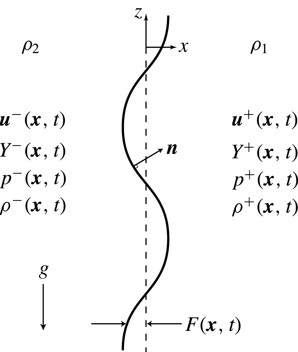
Here, we are interested in a variable-density linear inviscid instability where two vertical columns of different densities are accelerating due to the action of gravity. While one is tempted to think of the flow as an RT configuration, what we have is really a variable-density KH flow with accelerating free streams. Figure 1 illustrates the flow configuration and the Cartesian coordinate system used throughout the rest of this paper. A constant gravitational acceleration field
 $g$
is acting downwards (
 $-\hat{\boldsymbol{z}}$
direction), and the unperturbed interface is initially located along the
 $z$
-axis at
 $x=0$
. The densities of the left and right columns are
 $\unicode[STIX]{x1D70C}_{2}$
and
 $\unicode[STIX]{x1D70C}_{1}$
respectively. We define the following parameters for our subsequent discussion:
 $$\begin{eqnarray}R\equiv \frac{\unicode[STIX]{x1D70C}_{1}}{\unicode[STIX]{x1D70C}_{2}},\quad \bar{\unicode[STIX]{x1D70C}}\equiv \frac{\unicode[STIX]{x1D70C}_{1}+\unicode[STIX]{x1D70C}_{2}}{2},\end{eqnarray}$$
where
 $R$
is the density ratio of high- to low-density fluid and
 $\bar{\unicode[STIX]{x1D70C}}$
is the mean density. The analysis that follows explains the influence of discrete wavemodes and surface tension on the evolution of the interface amplitude and perturbation fields.
Planar sketch of the flow configuration in Cartesian coordinates (
 $y$
is perpendicular to the page).

2 Linear stability analysis
The flow obeys the Euler equations at each side of the interface,
 $$\begin{eqnarray}\displaystyle & \displaystyle \unicode[STIX]{x1D70C}\left(\frac{\unicode[STIX]{x2202}\boldsymbol{u}}{\unicode[STIX]{x2202}t}+\boldsymbol{u}\boldsymbol{\cdot }\unicode[STIX]{x1D735}\boldsymbol{u}\right)=-\unicode[STIX]{x1D735}p-(\unicode[STIX]{x1D70C}-\bar{\unicode[STIX]{x1D70C}})g\hat{\boldsymbol{z}}, & \displaystyle\end{eqnarray}$$
 $$\begin{eqnarray}\displaystyle & \displaystyle \frac{\unicode[STIX]{x2202}Y}{\unicode[STIX]{x2202}t}+\boldsymbol{u}\boldsymbol{\cdot }\unicode[STIX]{x1D735}Y=0, & \displaystyle\end{eqnarray}$$
 $$\begin{eqnarray}\displaystyle & \displaystyle \unicode[STIX]{x1D735}\boldsymbol{\cdot }\boldsymbol{u}=0, & \displaystyle\end{eqnarray}$$
where
 $\unicode[STIX]{x1D70C}$
is the density of the mixture,
 $\boldsymbol{u}=(u,v,w)$
is the velocity vector,
 $p$
is the pressure and
 $Y$
is the mass fraction of one of the species. There is no chemical reaction between the two streams. We note that the flow velocities are formulated in the frame of reference where the net vertical momentum is zero; see Gat et al. (Reference Gat, Matheou, Chung and Dimotakis2017). For a binary mixture in the zero-Mach-number limit (Sandoval Reference Sandoval1995), the density is related to the local mass fraction according to
 $$\begin{eqnarray}\frac{1}{\unicode[STIX]{x1D70C}(\boldsymbol{x},t)}=\left(\frac{1}{\unicode[STIX]{x1D70C}_{1}}-\frac{1}{\unicode[STIX]{x1D70C}_{2}}\right)Y(\boldsymbol{x},t)+\frac{1}{\unicode[STIX]{x1D70C}_{2}}\equiv \unicode[STIX]{x1D708}_{2}+\unicode[STIX]{x0394}\unicode[STIX]{x1D708}\,Y(\boldsymbol{x},t),\end{eqnarray}$$
where
 $$\begin{eqnarray}\unicode[STIX]{x0394}\unicode[STIX]{x1D708}=\left(\frac{1}{\unicode[STIX]{x1D70C}_{1}}-\frac{1}{\unicode[STIX]{x1D70C}_{2}}\right),\quad \unicode[STIX]{x1D708}_{i}=\frac{1}{\unicode[STIX]{x1D70C}_{i}}.\end{eqnarray}$$
We now introduce the following expansion for all flow fields:
 $$\begin{eqnarray}\displaystyle \unicode[STIX]{x1D6F9}(\boldsymbol{x},t)=\unicode[STIX]{x1D6F9}_{0}(x,t)+\unicode[STIX]{x1D716}\unicode[STIX]{x1D6F9}_{1}(\boldsymbol{x},t)+\unicode[STIX]{x1D716}^{2}\unicode[STIX]{x1D6F9}_{2}(\boldsymbol{x},t)+\cdots , & & \displaystyle\end{eqnarray}$$
where
 $\unicode[STIX]{x1D6F9}=\{u,v,w,Y,p\}$
and
 $\unicode[STIX]{x1D716}$
is small. The subscripts
 $0$
and
 $1$
denote the base flow and the first-order perturbation fields respectively.
The solution for the base flow is given by
 $$\begin{eqnarray}u_{0}=0,\quad v_{0}=0,\quad p_{0}=0,\end{eqnarray}$$
 $$\begin{eqnarray}\frac{\unicode[STIX]{x2202}Y_{0}}{\unicode[STIX]{x2202}t}=0,\quad \unicode[STIX]{x1D70C}_{0}=(\unicode[STIX]{x1D708}_{2}+\unicode[STIX]{x0394}\unicode[STIX]{x1D708}\,Y_{0})^{-1},\end{eqnarray}$$
 $$\begin{eqnarray}\frac{\unicode[STIX]{x2202}w_{0}}{\unicode[STIX]{x2202}t}=-\left(1-\frac{\bar{\unicode[STIX]{x1D70C}}}{\unicode[STIX]{x1D70C}_{0}}\right)g.\end{eqnarray}$$
From (2.8), we infer that
 $Y_{0}(x,t)=H(x)$
, where
 $H(x)$
denotes the Heaviside function, and subsequently from (2.4) and (2.9) we obtain
 $$\begin{eqnarray}\frac{\unicode[STIX]{x2202}w_{0}}{\unicode[STIX]{x2202}t}=-[1-\bar{\unicode[STIX]{x1D70C}}(\unicode[STIX]{x1D708}_{2}+\unicode[STIX]{x0394}\unicode[STIX]{x1D708}\,H(x))]g.\end{eqnarray}$$
Denoting
 $\pm$
as the right and left fields with respect to the interface respectively, we have from (2.10)
 $$\begin{eqnarray}w_{0}^{\pm }=\pm \frac{(1-R)}{2R^{\pm }}gt\equiv \mp 2a^{\pm }t,\end{eqnarray}$$
where
 $R^{+}=R$
and
 $R^{-}=1$
, and
 $$\begin{eqnarray}a^{\pm }\equiv \frac{(R-1)}{4R^{\pm }}g.\end{eqnarray}$$
Now, the equations for the first-order perturbation fields are
 $$\begin{eqnarray}\displaystyle & \displaystyle \frac{\unicode[STIX]{x2202}u_{1}}{\unicode[STIX]{x2202}t}+w_{0}(t)\frac{\unicode[STIX]{x2202}u_{1}}{\unicode[STIX]{x2202}z}=-\frac{1}{\unicode[STIX]{x1D70C}_{0}}\frac{\unicode[STIX]{x2202}p_{1}}{\unicode[STIX]{x2202}x}, & \displaystyle\end{eqnarray}$$
 $$\begin{eqnarray}\displaystyle & \displaystyle \frac{\unicode[STIX]{x2202}v_{1}}{\unicode[STIX]{x2202}t}+w_{0}(t)\frac{\unicode[STIX]{x2202}v_{1}}{\unicode[STIX]{x2202}z}=-\frac{1}{\unicode[STIX]{x1D70C}_{0}}\frac{\unicode[STIX]{x2202}p_{1}}{\unicode[STIX]{x2202}y}, & \displaystyle\end{eqnarray}$$
 $$\begin{eqnarray}\displaystyle & \displaystyle \frac{\unicode[STIX]{x2202}w_{1}}{\unicode[STIX]{x2202}t}+w_{0}(t)\frac{\unicode[STIX]{x2202}w_{1}}{\unicode[STIX]{x2202}z}=-\frac{1}{\unicode[STIX]{x1D70C}_{0}}\frac{\unicode[STIX]{x2202}p_{1}}{\unicode[STIX]{x2202}z}+\unicode[STIX]{x0394}\unicode[STIX]{x1D708}\,g\bar{\unicode[STIX]{x1D70C}}Y_{1}, & \displaystyle\end{eqnarray}$$
 $$\begin{eqnarray}\displaystyle & \displaystyle \frac{\unicode[STIX]{x2202}Y_{1}}{\unicode[STIX]{x2202}t}+w_{0}(t)\frac{\unicode[STIX]{x2202}Y_{1}}{\unicode[STIX]{x2202}z}=0, & \displaystyle\end{eqnarray}$$
 $$\begin{eqnarray}\displaystyle & \displaystyle \frac{\unicode[STIX]{x2202}u_{1}}{\unicode[STIX]{x2202}x}+\frac{\unicode[STIX]{x2202}v_{1}}{\unicode[STIX]{x2202}y}+\frac{\unicode[STIX]{x2202}w_{1}}{\unicode[STIX]{x2202}z}=0, & \displaystyle\end{eqnarray}$$
valid on both the left and the right of the interface. The fields obey different equations because
 $w_{0}(t)=w_{0}^{\pm }(t)$
is different on each side of the interface.
We now introduce Fourier modes along the homogeneous directions, according to
 $$\begin{eqnarray}(u_{1},v_{1},w_{1},Y_{1},p_{1})=(\hat{u} (x,t),\hat{v}(x,t),{\hat{w}}(x,t),{\hat{Y}}(x,t),\hat{p}(x,t))\text{e}^{\text{i}(ky+mz)}+\text{c.c.},\end{eqnarray}$$
where
 $k$
and
 $m$
are the wavenumbers of the disturbances in the
 $y$
- and
 $z$
-directions respectively. Equations (2.13)–(2.17) become
 $$\begin{eqnarray}\displaystyle & \displaystyle \frac{\unicode[STIX]{x2202}\hat{u} }{\unicode[STIX]{x2202}t}+\text{i}mw_{0}(t)\hat{u} =-\frac{1}{\unicode[STIX]{x1D70C}_{0}}\frac{\unicode[STIX]{x2202}\hat{p}}{\unicode[STIX]{x2202}x}, & \displaystyle\end{eqnarray}$$
 $$\begin{eqnarray}\displaystyle & \displaystyle \frac{\unicode[STIX]{x2202}\hat{v}}{\unicode[STIX]{x2202}t}+\text{i}mw_{0}(t)\hat{v}=-\frac{1}{\unicode[STIX]{x1D70C}_{0}}\text{i}k\hat{p}, & \displaystyle\end{eqnarray}$$
 $$\begin{eqnarray}\displaystyle & \displaystyle \frac{\unicode[STIX]{x2202}{\hat{w}}}{\unicode[STIX]{x2202}t}+\text{i}mw_{0}(t){\hat{w}}=-\frac{1}{\unicode[STIX]{x1D70C}_{0}}\text{i}m\hat{p}+\unicode[STIX]{x0394}\unicode[STIX]{x1D708}\,g\bar{\unicode[STIX]{x1D70C}}{\hat{Y}}, & \displaystyle\end{eqnarray}$$
 $$\begin{eqnarray}\displaystyle & \displaystyle \frac{\unicode[STIX]{x2202}{\hat{Y}}}{\unicode[STIX]{x2202}t}+\text{i}mw_{0}(t){\hat{Y}}=0, & \displaystyle\end{eqnarray}$$
 $$\begin{eqnarray}\displaystyle & \displaystyle \frac{\unicode[STIX]{x2202}\hat{u} }{\unicode[STIX]{x2202}x}+\text{i}k\hat{v}+\text{i}m{\hat{w}}=0. & \displaystyle\end{eqnarray}$$
The scalar equation (2.22) can be integrated immediately using (2.11)–(2.12) to
 $$\begin{eqnarray}{\hat{Y}}^{\pm }(x,t)={\hat{Y}}_{o}^{\pm }(x)\exp (\pm \text{i}ma^{\pm }t^{2}),\end{eqnarray}$$
and in order for
 ${\hat{Y}}$
to decay to zero at infinity, we must have
 ${\hat{Y}}_{o}^{\pm }(x)=0$
. A pressure equation can be derived by combining (2.19)–(2.21) with (2.23), giving
 $$\begin{eqnarray}-\frac{\unicode[STIX]{x2202}}{\unicode[STIX]{x2202}x}\left(\frac{1}{\unicode[STIX]{x1D70C}_{0}}\frac{\unicode[STIX]{x2202}\hat{p}}{\unicode[STIX]{x2202}x}\right)+\frac{k^{2}+m^{2}}{\unicode[STIX]{x1D70C}_{0}}\hat{p}=-\text{i}m\unicode[STIX]{x0394}\unicode[STIX]{x1D708}\,g\bar{\unicode[STIX]{x1D70C}}{\hat{Y}}.\end{eqnarray}$$
Using
 ${\hat{Y}}^{\pm }=0$
, equation (2.25) becomes
 $$\begin{eqnarray}-\frac{\text{d}^{2}\hat{p}^{\pm }}{\text{d}x^{2}}+(k^{2}+m^{2})\hat{p}^{\pm }=0,\end{eqnarray}$$
whose solution is
 $$\begin{eqnarray}\hat{p}^{\pm }=C_{0}^{\pm }(t)\text{e}^{\mp Kx},\end{eqnarray}$$
where
 $$\begin{eqnarray}K^{2}=k^{2}+m^{2},\end{eqnarray}$$
in which we have used the fact that
 $\hat{p}$
has to remain finite as
 $|x|\rightarrow \infty$
.
Now, the pressure and scalar fields are introduced into the momentum equations (2.19)–(2.21), showing that the general structure of the solutions is of the form
 $$\begin{eqnarray}\frac{\unicode[STIX]{x2202}\hat{\unicode[STIX]{x1D719}}^{\pm }}{\unicode[STIX]{x2202}t}\mp 2\text{i}ma^{\pm }t\hat{\unicode[STIX]{x1D719}}^{\pm }=C_{0}^{\pm }(t),\end{eqnarray}$$
where
 $$\begin{eqnarray}\hat{u} ^{\pm }=\pm \frac{K}{\unicode[STIX]{x1D70C}^{\pm }}\hat{\unicode[STIX]{x1D719}}^{\pm }\text{e}^{\mp Kx},\quad \hat{v}^{\pm }=-\frac{\text{i}k}{\unicode[STIX]{x1D70C}^{\pm }}\hat{\unicode[STIX]{x1D719}}^{\pm }\text{e}^{\mp Kx},\quad {\hat{w}}^{\pm }=-\frac{\text{i}m}{\unicode[STIX]{x1D70C}^{\pm }}\hat{\unicode[STIX]{x1D719}}^{\pm }\text{e}^{\mp Kx}.\end{eqnarray}$$
Equation (2.29) has the general solution
 $$\begin{eqnarray}\hat{\unicode[STIX]{x1D719}}^{\pm }(t)=\hat{\unicode[STIX]{x1D719}}_{0}^{\pm }\text{e}^{\pm \text{i}ma^{\pm }t^{2}}+\int _{0}^{t}C_{0}^{\pm }(t^{\prime })\text{e}^{\pm \text{i}ma^{\pm }(t^{2}-{t^{\prime }}^{2})}\,\text{d}t^{\prime },\end{eqnarray}$$
and in order for
 $\hat{\unicode[STIX]{x1D719}}^{\pm }$
to decay to zero at infinity, we must have
 $\hat{\unicode[STIX]{x1D719}}_{0}^{\pm }=0$
as before, which results finally in
 $$\begin{eqnarray}\hat{\unicode[STIX]{x1D719}}^{\pm }(t)=\int _{0}^{t}C_{0}^{\pm }(t^{\prime })\text{e}^{\pm \text{i}ma^{\pm }(t^{2}-{t^{\prime }}^{2})}\,\text{d}t^{\prime }.\end{eqnarray}$$
Subsequently, we consider the interface (see figure 1), here defined implicitly by
 $$\begin{eqnarray}F(x,y,z,t)=x-x_{f}(y,z,t)=0,\end{eqnarray}$$
where the subscript
 $f$
denotes interface quantities. From (2.33), we can calculate the normal, according to
 $$\begin{eqnarray}\boldsymbol{n}=\frac{\unicode[STIX]{x1D735}F}{|\unicode[STIX]{x1D735}F|}=\frac{1}{\sqrt{1+x_{f,y}^{2}+x_{f,z}^{2}}}(1,-x_{f,y},-x_{f,z}).\end{eqnarray}$$
Similarly, the velocity of the interface,
 $u_{f}$
, is given by
 $$\begin{eqnarray}\frac{\unicode[STIX]{x2202}F}{\unicode[STIX]{x2202}t}+u_{f}~\boldsymbol{n}\boldsymbol{\cdot }\unicode[STIX]{x1D735}F=\frac{\unicode[STIX]{x2202}F}{\unicode[STIX]{x2202}t}+u_{f}|\unicode[STIX]{x1D735}F|=0,\end{eqnarray}$$
which gives the normal velocity
 $$\begin{eqnarray}u_{f}=-\frac{\displaystyle \frac{\unicode[STIX]{x2202}F}{\unicode[STIX]{x2202}t}}{|\unicode[STIX]{x1D735}F|}=\frac{x_{f,t}}{\sqrt{1+x_{f,y}^{2}+x_{f,z}^{2}}}.\end{eqnarray}$$
The curvature of the interface is given by the standard formula
 $$\begin{eqnarray}\unicode[STIX]{x1D735}\boldsymbol{\cdot }\boldsymbol{n}=\frac{(x_{f,y}^{2}x_{f,yy}+x_{f,z}^{2}x_{f,zz})-(x_{f,yy}+x_{f,zz})(1+x_{f,y}^{2}+x_{f,z}^{2})}{(1+x_{f,y}^{2}+x_{f,z}^{2})^{3/2}}.\end{eqnarray}$$
The jump conditions at the interface are
 $$\begin{eqnarray}\displaystyle & \displaystyle -u_{f}[\unicode[STIX]{x1D70C}]+[\unicode[STIX]{x1D70C}u_{n}]=0, & \displaystyle\end{eqnarray}$$
 $$\begin{eqnarray}\displaystyle & \displaystyle -u_{f}[\unicode[STIX]{x1D70C}Y]+[\unicode[STIX]{x1D70C}Yu_{n}]=0, & \displaystyle\end{eqnarray}$$
 $$\begin{eqnarray}\displaystyle & \displaystyle -u_{f}[\unicode[STIX]{x1D70C}u_{n}]+[\unicode[STIX]{x1D70C}u_{n}^{2}+p]=-\unicode[STIX]{x1D70E}\unicode[STIX]{x1D735}\boldsymbol{\cdot }\boldsymbol{n}, & \displaystyle\end{eqnarray}$$
 $$\begin{eqnarray}\displaystyle & \displaystyle -u_{f}[\unicode[STIX]{x1D70C}u_{t1}]+[\unicode[STIX]{x1D70C}u_{n}u_{t1}]=0, & \displaystyle\end{eqnarray}$$
 $$\begin{eqnarray}\displaystyle & \displaystyle -u_{f}[\unicode[STIX]{x1D70C}u_{t2}]+[\unicode[STIX]{x1D70C}u_{n}u_{t2}]=0, & \displaystyle\end{eqnarray}$$
where
 $\unicode[STIX]{x1D70E}$
is the interfacial surface tension,
 $u_{n}$
,
 $u_{t1}$
and
 $u_{t2}$
are the normal and tangential velocity components respectively and square brackets denote the jump across the interface. We now introduce the expansions
 $$\begin{eqnarray}\left.\begin{array}{@{}c@{}}\displaystyle x_{f}=\unicode[STIX]{x1D716}\unicode[STIX]{x1D701}+O(\unicode[STIX]{x1D716}^{2}),\quad \boldsymbol{n}=(1,-\unicode[STIX]{x1D716}\unicode[STIX]{x1D701}_{y},-\unicode[STIX]{x1D716}\unicode[STIX]{x1D701}_{z})+O(\unicode[STIX]{x1D716}^{2}),\\ \displaystyle \boldsymbol{t}_{1}=(\unicode[STIX]{x1D716}\unicode[STIX]{x1D701}_{y},1,0)+O(\unicode[STIX]{x1D716}^{2}),\quad \boldsymbol{t}_{2}=(\unicode[STIX]{x1D716}\unicode[STIX]{x1D701}_{z},0,1)+O(\unicode[STIX]{x1D716}^{2}),\\ \displaystyle u_{f}=\unicode[STIX]{x1D716}\unicode[STIX]{x1D701}_{t}+O(\unicode[STIX]{x1D716}^{2}),\quad \unicode[STIX]{x1D735}\boldsymbol{\cdot }\boldsymbol{n}=-\unicode[STIX]{x1D716}(\unicode[STIX]{x1D701}_{yy}+\unicode[STIX]{x1D701}_{zz})+O(\unicode[STIX]{x1D716}^{2})\end{array}\right\}\end{eqnarray}$$
and
 $$\begin{eqnarray}\displaystyle & \displaystyle u_{n}=(\unicode[STIX]{x1D716}u_{1},\unicode[STIX]{x1D716}v_{1},w_{0}(t)+\unicode[STIX]{x1D716}w_{1})\cdot (1,-\unicode[STIX]{x1D716}\unicode[STIX]{x1D701}_{y},-\unicode[STIX]{x1D716}\unicode[STIX]{x1D701}_{z})=\unicode[STIX]{x1D716}(u_{1}-w_{0}(t)\unicode[STIX]{x1D701}_{z})+O(\unicode[STIX]{x1D716}^{2}), & \displaystyle\end{eqnarray}$$
 $$\begin{eqnarray}\displaystyle & \displaystyle u_{t_{1}}=(\unicode[STIX]{x1D716}u_{1},\unicode[STIX]{x1D716}v_{1},w_{0}(t)+\unicode[STIX]{x1D716}w_{1})\cdot (\unicode[STIX]{x1D716}\unicode[STIX]{x1D701}_{y},1,0)=\unicode[STIX]{x1D716}v_{1}+O(\unicode[STIX]{x1D716}^{2}), & \displaystyle\end{eqnarray}$$
 $$\begin{eqnarray}\displaystyle & \displaystyle u_{t_{2}}=(\unicode[STIX]{x1D716}u_{1},\unicode[STIX]{x1D716}v_{1},w_{0}(t)+\unicode[STIX]{x1D716}w_{1})\cdot (\unicode[STIX]{x1D716}\unicode[STIX]{x1D701}_{z},0,1)=w_{0}(t)+\unicode[STIX]{x1D716}w_{1}+O(\unicode[STIX]{x1D716}^{2}). & \displaystyle\end{eqnarray}$$
Introducing (2.43)–(2.46) into (2.38)–(2.42), expanding all quantities around
 $x=0$
and gathering terms up to first order in
 $\unicode[STIX]{x1D716}$
results in
 $$\begin{eqnarray}\displaystyle & \displaystyle [p_{1}]=\unicode[STIX]{x1D70E}(\unicode[STIX]{x1D701}_{yy}+\unicode[STIX]{x1D701}_{zz}), & \displaystyle\end{eqnarray}$$
 $$\begin{eqnarray}\displaystyle & \displaystyle u_{1}^{\pm }-w_{0}^{\pm }(t)\unicode[STIX]{x1D701}_{z}=\unicode[STIX]{x1D701}_{t}. & \displaystyle\end{eqnarray}$$
 $$\begin{eqnarray}C_{0}^{+}(t)=C_{0}^{-}(t)-\unicode[STIX]{x1D70E}K^{2}\hat{\unicode[STIX]{x1D701}},\end{eqnarray}$$
and, similarly, equation (2.47b ) becomes
 $$\begin{eqnarray}\frac{\unicode[STIX]{x2202}\hat{\unicode[STIX]{x1D701}}}{\unicode[STIX]{x2202}t}\mp 2\text{i}ma^{\pm }t\hat{\unicode[STIX]{x1D701}}=\hat{u} ^{\pm }(x=0)=\pm \frac{K}{\unicode[STIX]{x1D70C}^{\pm }}\left[\int _{0}^{t}C_{0}^{\pm }(t^{\prime })\text{e}^{\pm \text{i}ma^{\pm }(t^{2}-{t^{\prime }}^{2})}\,\text{d}t^{\prime }\right].\end{eqnarray}$$
At this point, we have three equations with three unknowns,
 $\hat{\unicode[STIX]{x1D701}}$
and
 ${\hat{C}}_{0}^{\pm }$
. Multiplying (2.49) by
 $\text{e}^{\mp \text{i}ma^{\pm }t^{2}}$
, taking the derivative with respect to time, cancelling exponential terms on both sides and eliminating
 $C_{0}^{\pm }$
using (2.48), we obtain
 $$\begin{eqnarray}\frac{\text{d}^{2}\hat{\unicode[STIX]{x1D701}}}{\text{d}t^{2}}+\left(\unicode[STIX]{x1D6FD}_{0}^{2}-\frac{\unicode[STIX]{x1D714}_{0}^{4}}{4}t^{2}\right)\hat{\unicode[STIX]{x1D701}}(t)=0,\end{eqnarray}$$
with
 $$\begin{eqnarray}\unicode[STIX]{x1D6FD}_{0}^{2}=\frac{K^{3}\unicode[STIX]{x1D70E}}{\unicode[STIX]{x1D70C}^{+}+\unicode[STIX]{x1D70C}^{-}},\quad \unicode[STIX]{x1D714}_{0}^{4}=g^{2}m^{2}\frac{(R-1)^{2}}{R}.\end{eqnarray}$$
Equation (2.50a
) can be non-dimensionalized by introducing
 $\unicode[STIX]{x1D70F}\equiv \unicode[STIX]{x1D714}_{0}t$
and defining a dimensionless parameter
 $$\begin{eqnarray}\unicode[STIX]{x1D708}=\frac{\unicode[STIX]{x1D6FD}_{0}^{2}}{\unicode[STIX]{x1D714}_{0}^{2}}=\frac{\sqrt{(k^{2}+m^{2})^{3}}\unicode[STIX]{x1D70E}\sqrt{R}}{(\unicode[STIX]{x1D70C}^{+}+\unicode[STIX]{x1D70C}^{-})(R-1)gm},\end{eqnarray}$$
giving
 $$\begin{eqnarray}\frac{\text{d}^{2}\hat{\unicode[STIX]{x1D701}}}{\text{d}\unicode[STIX]{x1D70F}^{2}}-\left(\frac{1}{4}\unicode[STIX]{x1D70F}^{2}-\unicode[STIX]{x1D708}\right)\hat{\unicode[STIX]{x1D701}}(\unicode[STIX]{x1D70F})=0.\end{eqnarray}$$
The general solution of (2.52) can be expressed, see Abramowitz & Stegun (Reference Abramowitz and Stegun1965), as
 $$\begin{eqnarray}\hat{\unicode[STIX]{x1D701}}(\unicode[STIX]{x1D70F})=C_{1}D_{\unicode[STIX]{x1D708}-1/2}(\unicode[STIX]{x1D70F})+C_{2}D_{-\unicode[STIX]{x1D708}-1/2}(\text{i}\unicode[STIX]{x1D70F}),\end{eqnarray}$$
where
 $D_{a}(z)$
denotes the parabolic cylinder function of order
 $a$
. (It should be noted that although an imaginary argument is used in the second term of (2.53), the complete result is real after the constants are determined.) By enforcing the initial conditions
 $\hat{\unicode[STIX]{x1D701}}=1$
and
 $\hat{\unicode[STIX]{x1D701}}_{\unicode[STIX]{x1D70F}}=0$
(obtained by setting
 $t=0$
in (2.49)), we get
 $$\begin{eqnarray}C_{1}=-\text{i}2^{-\unicode[STIX]{x1D708}}\frac{\unicode[STIX]{x1D6E4}\displaystyle \left(-\frac{\unicode[STIX]{x1D708}}{2}+\frac{1}{4}\right)}{\unicode[STIX]{x1D6E4}\displaystyle \left(\frac{\unicode[STIX]{x1D708}}{2}+\frac{1}{4}\right)}C_{2}\end{eqnarray}$$
and
 $$\begin{eqnarray}C_{2}=\frac{(1+\text{i})}{\unicode[STIX]{x03C0}}2^{-7/4-\unicode[STIX]{x1D708}/2}\text{e}^{-\text{i}\unicode[STIX]{x03C0}\unicode[STIX]{x1D708}/2}(1+\text{e}^{2\text{i}\unicode[STIX]{x03C0}\unicode[STIX]{x1D708}})\unicode[STIX]{x1D6E4}\left(-\frac{\unicode[STIX]{x1D708}}{2}+\frac{3}{4}\right)\unicode[STIX]{x1D6E4}\left(\unicode[STIX]{x1D708}+\frac{1}{2}\right).\end{eqnarray}$$
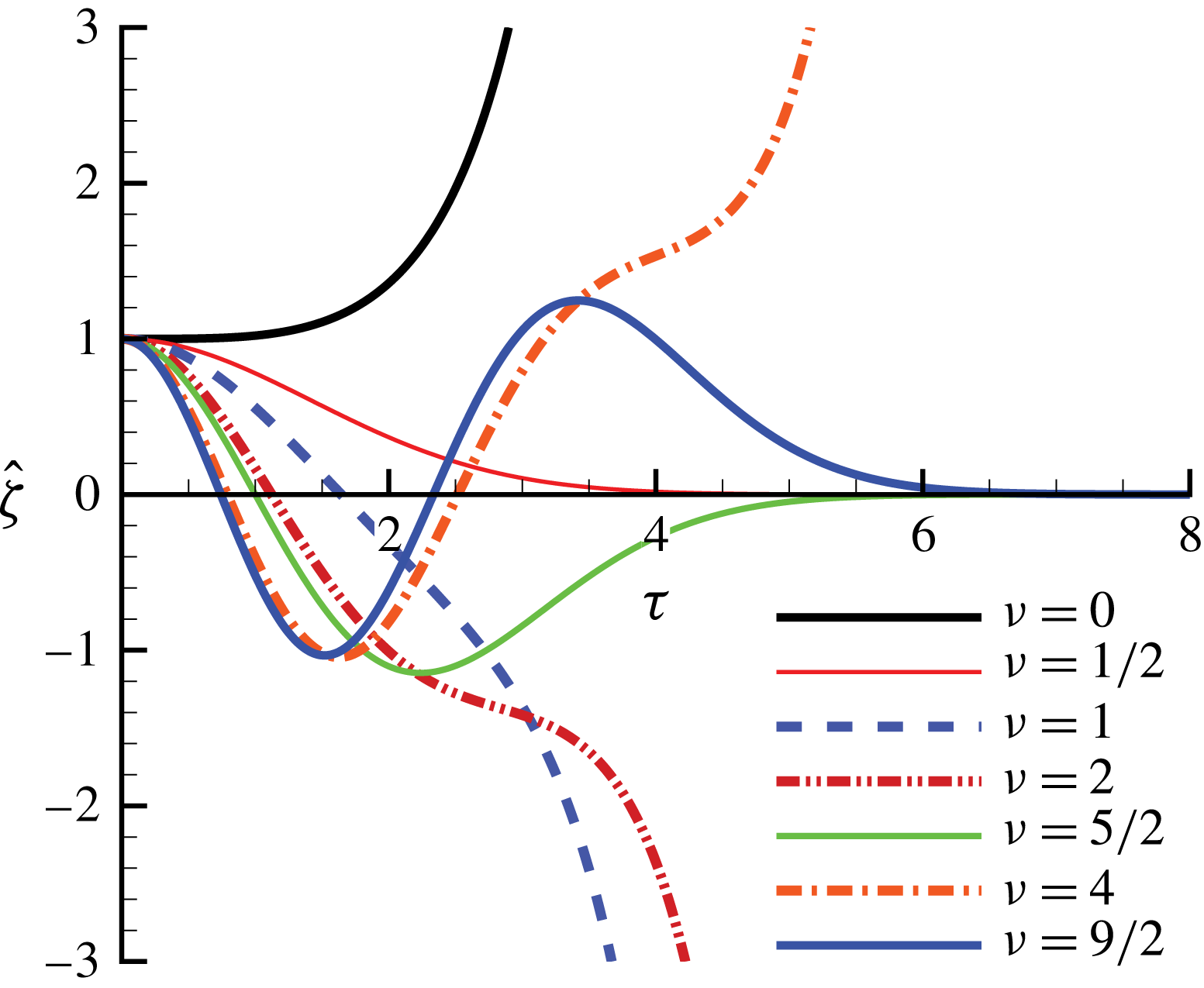
Evolution of the interface amplitude
 $\hat{\unicode[STIX]{x1D701}}$
for various values of
 $\unicode[STIX]{x1D708}$
.

We will discuss here the general behaviour of
 $\hat{\unicode[STIX]{x1D701}}(\unicode[STIX]{x1D70F})$
, and postpone to the next section a more detailed consideration of the asymptotic dependence for large
 $\unicode[STIX]{x1D70F}$
. Figure 2 shows
 $\hat{\unicode[STIX]{x1D701}}(\unicode[STIX]{x1D70F})$
obtained by plotting (2.53) for various values of
 $\unicode[STIX]{x1D708}$
; the results were also verified by direct numerical integration of (2.52). First, it is observed that the interface is unconditionally unstable, with the most unstable behaviour for
 $\unicode[STIX]{x1D708}=0$
(a result that is expected given the stabilizing effect that surface tension has on this type of flow). Second, we observe that
 $\hat{\unicode[STIX]{x1D701}}$
decays for the particular values
 $\unicode[STIX]{x1D708}_{n}=2n+1/2$
, where
 $n$
is an integer or zero, but this does not imply that the interface is stable. For these particular values, one arrives at a situation where the interface amplitude and its velocity both approach zero asymptotically for large
 $\unicode[STIX]{x1D70F}$
. In this hypothetical single-wavemode arrangement, the interface has been flattened and no further evolution is possible. Evidently, this behaviour will not arise if more wavemodes are present. The root of this unusual behaviour can be traced back to the time-dependent coefficient of (2.52), which generates solutions that have no counterpart in constant-coefficient ordinary differential equations. For example, this behaviour is not observed in LSA where harmonic solutions exist (normal modes). Third, one observes that
 $\hat{\unicode[STIX]{x1D701}}$
is not monotonically increasing (or decreasing). The amplitude magnitude generally shows an oscillatory behaviour (with a growing envelope). When
 $\unicode[STIX]{x1D70F}^{2}<4\unicode[STIX]{x1D708}$
, the coefficient multiplying
 $\hat{\unicode[STIX]{x1D701}}$
is negative and the solution is oscillatory-like. For large times,
 $\unicode[STIX]{x1D70F}^{2}>4\unicode[STIX]{x1D708}$
, the growth is exponential-like since the coefficient in the second term of the differential equation is positive. In addition, as happens in other shear flows, the most unstable growth happens for the two-dimensional mode (
 $k=0$
), suggesting similarity to Squire’s theorem (Squire Reference Squire1933) (although here we are concerned with a non-harmonic linear stability problem). Finally, the mismatch between the temporal phases of the fields on the two sides of the interface,
 $m(a^{+}+a^{-})t^{2}$
, grows with time quadratically, and there is no uniform phase-velocity translation where the interface appears fixed.
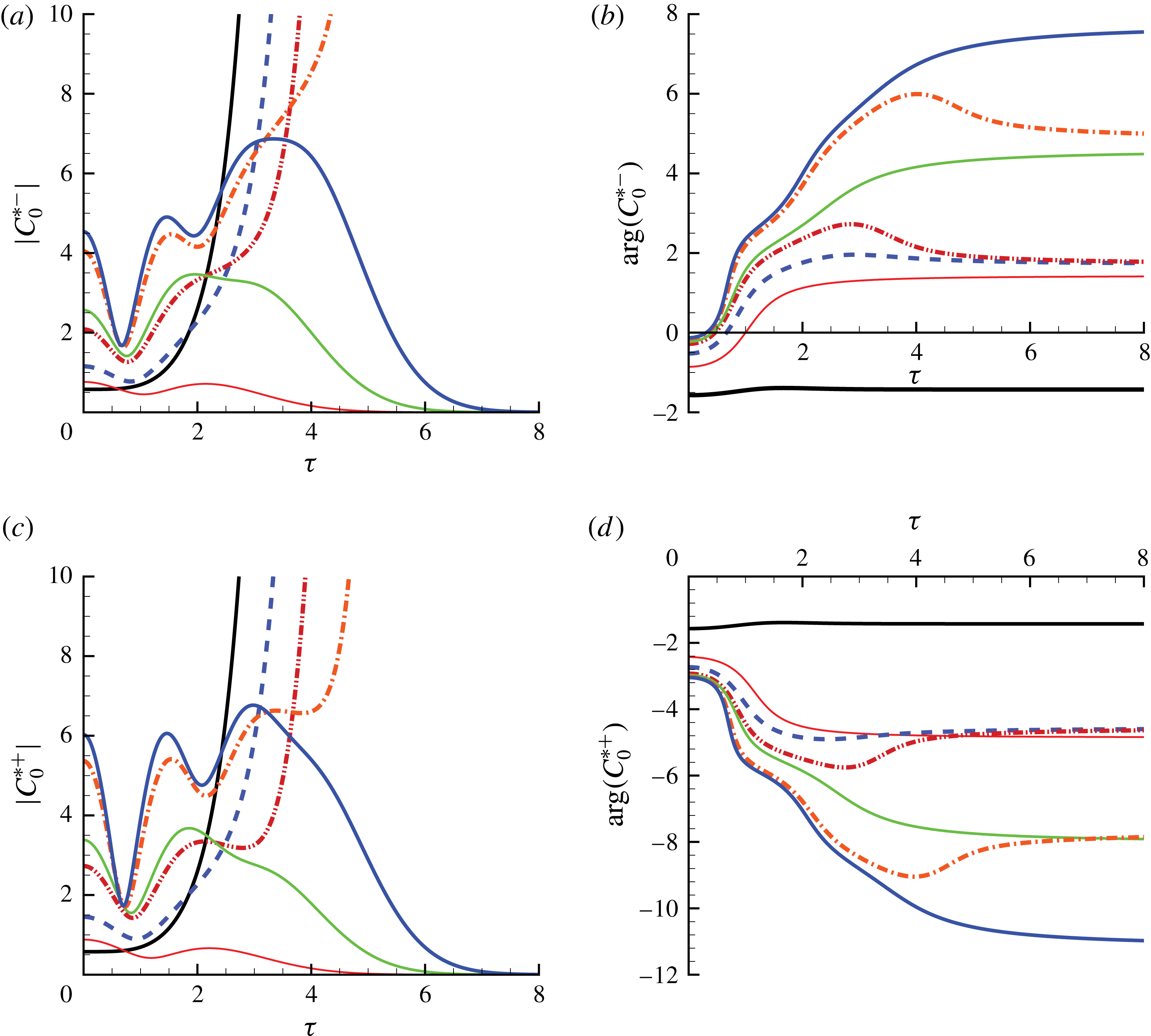
Magnitudes (a,c) and phases (b,d) of
 $C_{0}^{\ast -}$
and
 $C_{0}^{\ast +}$
for density ratio
 $R=4/3$
for various values of
 $\unicode[STIX]{x1D708}$
; legend as in figure 2.

Another quantity of interest is the pressure at the interface, which to leading order is equal to
 $C_{0}^{\pm }$
. Figure 3 shows the non-dimensional
 $$\begin{eqnarray}C_{0}^{\ast -}=\frac{KC_{0}^{-}(\unicode[STIX]{x1D70F})}{\unicode[STIX]{x1D714}_{0}^{2}\unicode[STIX]{x1D70C}^{-}}=\frac{\sqrt{R}}{4}\left[\left(\sqrt{R}\unicode[STIX]{x1D70F}^{2}-2\text{i}\right)\hat{\unicode[STIX]{x1D701}}(\unicode[STIX]{x1D70F})-4\text{i}\unicode[STIX]{x1D70F}\frac{\text{d}\hat{\unicode[STIX]{x1D701}}}{\text{d}\unicode[STIX]{x1D70F}}\right]-\frac{\text{d}^{2}\hat{\unicode[STIX]{x1D701}}}{\text{d}\unicode[STIX]{x1D70F}^{2}}\end{eqnarray}$$
and
 $C_{0}^{\ast +}(\unicode[STIX]{x1D70F})=C_{0}^{\ast -}(\unicode[STIX]{x1D70F})-\unicode[STIX]{x1D708}(R+1)\hat{\unicode[STIX]{x1D701}}$
, inferred from (2.48), as a function of time for different values of
 $\unicode[STIX]{x1D708}$
and density ratio
 $R=4/3$
(the behaviour is similar for other values of
 $R$
). Panels (a) and (c) show the magnitudes of the complex pressure intensities while panels (b) and (d) show their phases. It is observed that the pressure coefficient grows faster for
 $\unicode[STIX]{x1D708}=0$
, consistent with what is observed for
 $\hat{\unicode[STIX]{x1D701}}$
. The initial values can be determined analytically, giving
 $C_{0}^{\ast -}(0)=\unicode[STIX]{x1D708}-\text{i}\sqrt{R}/2$
and
 $C_{0}^{\ast +}(0)=-\unicode[STIX]{x1D708}R-\text{i}\sqrt{R}/2$
.
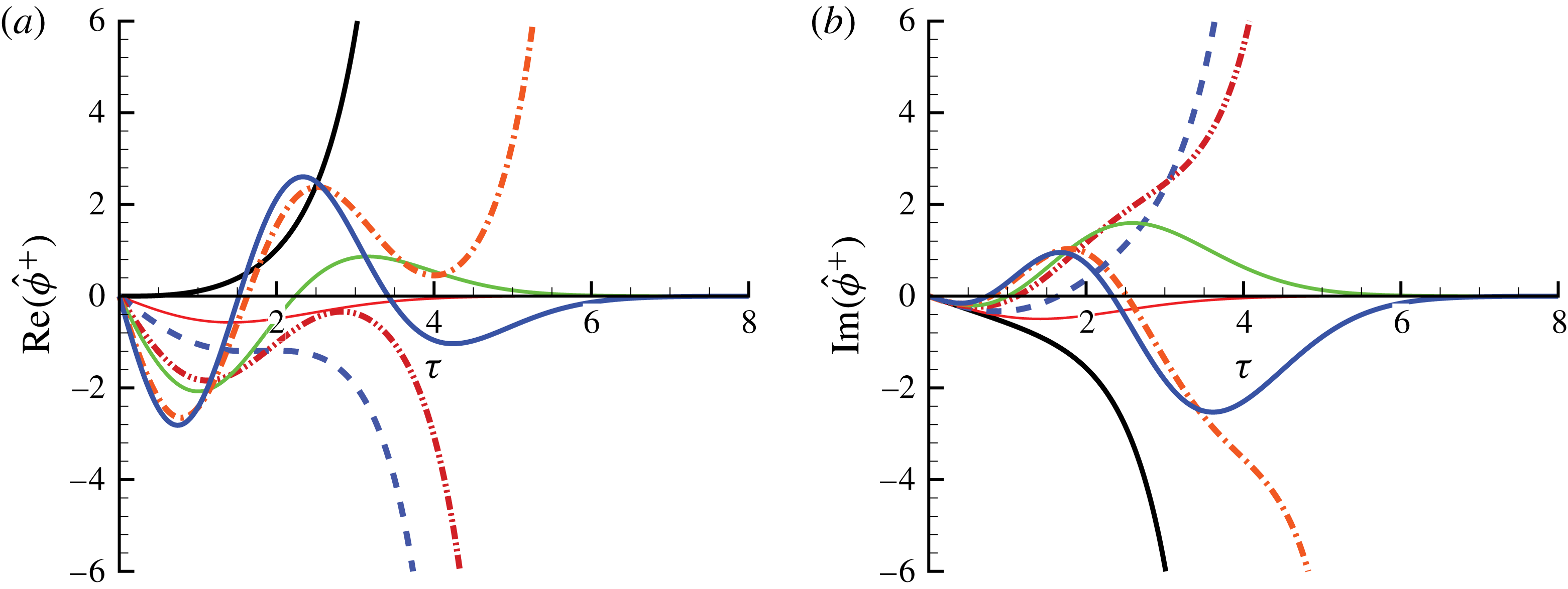
Finally, for completeness, figure 4 shows the real and imaginary parts of
 $\unicode[STIX]{x1D719}^{+}$
(
 $\unicode[STIX]{x1D719}^{-}$
is similar) as a function of time for different values of
 $\unicode[STIX]{x1D708}$
at
 $R=4/3$
. Evidently, these are also divergent functions of time.
Real and imaginary values of
 $\hat{\unicode[STIX]{x1D719}}^{+}$
for density ratio
 $R=4/3$
and various values of
 $\unicode[STIX]{x1D708}$
; legend as in figure 2.

3 Discussion
As discussed earlier, this flow is unconditionally unstable at all wavemodes, even in the presence of surface tension, because of the ever increasing (accelerating) momentum of the free streams. We did note that the interface amplitude can decay to zero for particular values of
 $\unicode[STIX]{x1D708}=\unicode[STIX]{x1D708}_{n}=2n+1/2$
, for
 $n=0,1,2,\ldots .$
It should first be noted that these particular values of
 $\unicode[STIX]{x1D708}$
are inconsequential because for given
 $\unicode[STIX]{x1D70E}$
there are always other wavemodes that are unstable. To clarify that this is the case in general, we can study the asymptotic behaviour of the solution for large
 $\unicode[STIX]{x1D70F}$
, using the known asymptotic expansions of the parabolic cylinder functions (see Abramowitz & Stegun Reference Abramowitz and Stegun1965), which results in
 $$\begin{eqnarray}\displaystyle \hat{\unicode[STIX]{x1D701}}(\unicode[STIX]{x1D70F}) & {\approx} & \displaystyle \text{}C_{1}\text{e}^{-\unicode[STIX]{x1D70F}^{2}/4}\unicode[STIX]{x1D70F}^{\unicode[STIX]{x1D708}-1/2}\left[1-\frac{(-\unicode[STIX]{x1D708}+\frac{1}{2})(-\unicode[STIX]{x1D708}+\frac{3}{2})}{2\unicode[STIX]{x1D70F}^{2}}\right.\nonumber\\ \displaystyle & & \displaystyle \left.+\,\frac{(-\unicode[STIX]{x1D708}+\frac{1}{2})(-\unicode[STIX]{x1D708}+\frac{3}{2})(-\unicode[STIX]{x1D708}+\frac{5}{2})(-\unicode[STIX]{x1D708}+\frac{7}{2})}{2\times 4\unicode[STIX]{x1D70F}^{4}}-\cdots \,\right]\nonumber\\ \displaystyle & & \displaystyle +\,C_{2}\text{e}^{\unicode[STIX]{x1D70F}^{2}/4}(\text{i}\unicode[STIX]{x1D70F})^{-\unicode[STIX]{x1D708}-1/2}\left[1+\frac{(\unicode[STIX]{x1D708}+\frac{1}{2})(\unicode[STIX]{x1D708}+\frac{3}{2})}{2\unicode[STIX]{x1D70F}^{2}}\right.\nonumber\\ \displaystyle & & \displaystyle \left.+\,\frac{(\unicode[STIX]{x1D708}+\frac{1}{2})(\unicode[STIX]{x1D708}+\frac{3}{2})(\unicode[STIX]{x1D708}+\frac{5}{2})(\unicode[STIX]{x1D708}+\frac{7}{2})}{2\times 4\unicode[STIX]{x1D70F}^{4}}+\cdots \,\right].\end{eqnarray}$$
Potential growth in the solution is only possible through the quadratic exponential term in the third and fourth lines of (3.1) which is multiplied by
 $C_{2}$
. Therefore, decay of the interface amplitude is only possible if
 $C_{2}=0$
. From (2.55), we see that this can only happen when
 $\text{e}^{\text{i}2\unicode[STIX]{x03C0}\unicode[STIX]{x1D708}}=-1$
, which explains the condition
 $\unicode[STIX]{x1D708}_{n}=2n+1/2$
. We also observe from the asymptotic behaviour that the dominant growth in time of
 $\hat{\unicode[STIX]{x1D701}}$
is of the form
 $$\begin{eqnarray}\hat{\unicode[STIX]{x1D701}}\sim \text{e}^{\unicode[STIX]{x1D70F}^{2}/4}\unicode[STIX]{x1D70F}^{-\unicode[STIX]{x1D708}-1/2}.\end{eqnarray}$$
4 Conclusion
The LSA of two fluid columns with different densities in a gravitational field has been carried out in the inviscid limit in the presence of surface tension. In this configuration, a uniform gravity field acts in the direction transverse to the density stratification, resulting in opposing constant acceleration of the free streams. The stability analysis is developed in the framework of an IVP, since the problem does not admit harmonic normal modes, and solved analytically. The results demonstrate that the flow is unconditionally unstable, due to the growing momentum of the free streams with time. Furthermore, the growth of the solution is quadratic in time exponential.
Acknowledgements
This work was supported in part by the Department of Energy, National Nuclear Security Administration, under award no. DE-NA0002382, and the California Institute of Technology. We are indebted to Professor P. E. Dimotakis for recommending that we study this problem.