INTRODUCTION
Determining the nature and timing of climatic and environmental changes across the Australian continent during the late last glacial stage (herein defined as 35,000–15,000 calendar years BP; 35–15 ka) has remained elusive. The timing of the coldest period during the last glacial stage, when global sea-level minimum and marine oxygen isotope maximum occurred (Hughes et al., Reference Hughes, Gibbard and Ehlers2013), is known as the last glacial maximum (LGM) (Clark et al., Reference Clark, Dyke, Shakun, Carlson, Clark, Wohlfarth and Mitrovica2009), within Marine Isotope Stage 2 (MIS 2) (29,000–14,000 years ago) (Lisiecki and Raymo, Reference Lisiecki and Raymo2005). Early definitions of the LGM suggested the global ice maximum and sea-level minimum occurred between 23–19 ka, during MIS 2 (Yokoyama et al., Reference Yokoyama, Lambeck, De Deckker, Johnston and Fifield2000; Mix, Bard and Schneider, Reference Mix, Bard and Schneider2001; Clark and Mix, Reference Clark and Mix2002). Increasingly, global evidence indicates that sea levels declined during late MIS 3 and global ice volume, including many mountain glaciers and continental ice sheets, reached their maximum extent prior to this period (Peltier and Fairbanks, Reference Peltier and Fairbanks2006; Clark et al., Reference Clark, Dyke, Shakun, Carlson, Clark, Wohlfarth and Mitrovica2009; Hughes et al., Reference Hughes, Gibbard and Ehlers2013; Lambeck et al., Reference Lambeck, Rouby, Purcell, Sun and Sambridge2014; Yokoyama et al., Reference Yokoyama, Esat, Thompson, Thomas, Webster, Miyairi and Sawada2018). This growing consensus has contributed to a widely accepted revision on the ice volume definition of the LGM as having occurred earlier, between 26.5–19 ka (Clark et al., Reference Clark, Dyke, Shakun, Carlson, Clark, Wohlfarth and Mitrovica2009; Hughes et al., Reference Hughes, Gibbard and Ehlers2013; Lambeck et al., Reference Lambeck, Rouby, Purcell, Sun and Sambridge2014). Whilst the timing of the occurrence of maximum global ice volume and minimum sea level has been refined, spatial variations in the occurrence of the coldest temperatures or maximum local glacial growth have been observed, particularly in the Southern Hemisphere. For Australia, the period of maximum environmental change has not been objectively defined.
Environmental changes during the LGM are characterised differently in Australia, where glacier development was a relatively minor component of the landscape, compared to the Northern Hemisphere. During the latter part of the last glacial stage and global sea-level minimum, various records from Australia document a period of low temperature, combined in many regions with more arid and highly variable climates (Miller et al., Reference Miller, Magee and Jull1997; Builth et al., Reference Builth, Kershaw, White, Roach, Hartney, McKenzie, Lewis and Jacobsen2008; Petherick et al., Reference Petherick, McGowan and Moss2008; Fletcher and Thomas, Reference Fletcher and Thomas2010; Fitzsimmons et al., Reference Fitzsimmons, Stern, Murray-Wallace, Truscott and Pop2015; Williams et al., Reference Williams, Veth, Steffen, Ulm, Turney, Reeves, Phipps and Smith2015; Miller et al., Reference Miller, Fogel, Magee and Gagan2016; Falster et al., Reference Falster, Tyler, Grant, Tibby, Turney, Löhr, Jacobsen and Kershaw2018). Temperatures in Australia during the last glacial stage are suggested to have been 4–8°C cooler than today (Miller et al., Reference Miller, Magee and Jull1997; Colhoun et al., Reference Colhoun, Pola, Barton and Heijnis1999; Colhoun, Reference Colhoun2000; Fletcher and Thomas, Reference Fletcher and Thomas2010; Woltering et al., Reference Woltering, Atahan, Grice, Heijnis, Taffs and Dodson2014; Chang et al., Reference Chang, Shulmeister, Woodward, Steinberger, Tibby and Barr2015). Temperature decreases of this magnitude are consistent with large changes to vegetation composition across the continent. Quantitative estimates of precipitation changes during the last glacial stage in Australia are limited; however, increased dust transport, sparse vegetation cover and the presence of sedimentary hiatuses in a range of lacustrine and palustrine sequences during this period (Supplementarly Figure 1; McKenzie, Reference McKenzie2002; Donders et al., Reference Donders, Wagner and Visscher2006; Williams et al., Reference Williams, Harle, Gale and Heijnis2006) may indicate a decrease in precipitation and thus an increase in aridity in some regions.
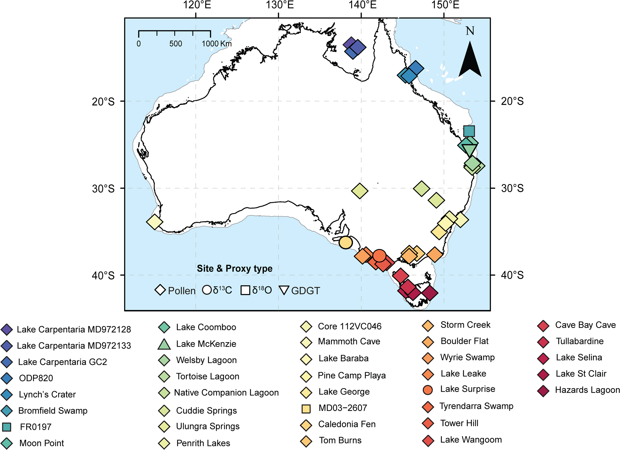
Map of Australia with sites indicated. Symbols show proxy type and colours indicate site locations. Colours change along a latitudinal gradient. Solid black line indicates the current extent of the Australian land mass and light grey line indicates the -130 m contour and the likely extent of exposed continental shelf during the global last glacial maximum. (For interpretation of the references to color in this figure legend, the reader is referred to the web version of this article.)

The spatial extent of such climate changes has remained a matter of debate, in part due to the geographic scale and range of climate regions across the Australian continent. The limited glacial activity and inferred increase in aridity during this period limits the number of high-resolution palaeoenvironmental archives across Australia, resulting in uncertainty in the interpretation and timing of climatic changes during the traditional LGM period. Whilst having experienced limited glacial activity, the Australian landmass and ensuing climates are strongly affected by variations in global temperature, sea level, pCO2 and Southern Ocean sea-ice extent. Therefore, major continental climate changes in Australia were likely to have been linked to changes in global ice volume through various teleconnections and feedbacks. In addition, the Australian land surface plays a poorly defined role in the global climate system, primarily via the production and export of dust and its role as a global sink/source of carbon, via soils and the terrestrial biosphere (De Deckker et al., Reference De Deckker, Norman, Goodwin, Wain and Gingele2010; Haverd et al., Reference Haverd, Raupach, Briggs, Canadell, Davis, Law and Meyer2013a; Haverd et al., Reference Haverd, Raupach, Briggs, Canadell, Isaac, Pickett-Heaps and Roxburgh2013b; Poulter et al., Reference Poulter, Frank, Ciais, Myneni, Andela, Bi and Broquet2014). The extent to which the Australian land surface exerted feedbacks on climate variability during the LGM remains a point of significant uncertainty.
Evidence for glacial and periglacial activity in Australia is restricted to high elevation sites in the Snowy Mountains of mainland southeastern Australia and in Tasmania (Barrows et al., Reference Barrows, Stone, Fifield and Cresswell2001, 2002; Mackintosh et al., Reference Mackintosh, Barrows, Colhoun and Fifield2006; Kiernan et al,, Reference Kiernan, Fink and McConnell2017). In the Snowy Mountains, the oldest moraines are most likely MIS 3 or MIS 4 in age, with later glacial advances occurring between 23 and 20 ka (recalcuated from Barrows et al., Reference Barrows, Stone, Fifield and Cresswell2001, 2002). Glaciation was more extensive in Tasmania, with evidence of numerous cirque, valley, and small ice sheet glaciations preserved at high elevation sites along the West Coast Range and the Central Plateau (Barrows et al., Reference Barrows, Stone, Fifield and Cresswell2002; Mackintosh et al., Reference Mackintosh, Barrows, Colhoun and Fifield2006). Exposure dating of moraines indicates that ice masses formed gradually from ca. 30 ka, with their maximum extent peaking at ca. 23–0 ka (Fink et al., Reference Fink, McKelvey, Hannan and Newsome2000; Barrows et al., Reference Barrows, Stone, Fifield and Cresswell2002; Kiernan et al, Reference Kiernan, Fifield and Chappell2004; Mackintosh et al., Reference Mackintosh, Barrows, Colhoun and Fifield2006; Kiernan et al., Reference Kiernan, Fink and McConnell2017). However, in several localities such as lower altitude sites in the West Coast Ranges, Mt. Field, and the Central Plateau, more extensive ice advances occurred during MIS 3 and MIS 4 (Fink et al., Reference Fink, McKelvey, Hannan and Newsome2000; Barrows et al., Reference Barrows, Stone, Fifield and Cresswell2002; Mackintosh et al., Reference Mackintosh, Barrows, Colhoun and Fifield2006). Deglaciation occurred rapidly after the global LGM, with the majority of ice cover disappearing between ca. 19–17 ka (Barrows et al., Reference Barrows, Stone, Fifield and Cresswell2002).
Continuous palaeoclimate records from lowland continental Australia during the last glacial stage are predominately based on qualitative proxy records, in particular pollen archived in lacustrine and palustrine sediments. Climate reconstructions from pollen records are rarely rigorously quantitative due to the low taxonomic resolution and large climatic envelopes of many Australian taxa. However, under present day CO2 and temperature conditions, vegetation in Australia is largely sensitive to water availability (Seddon et al., Reference Seddon, Macias-Fauria, Long, Benz and Willis2016). Biome distributions are strongly constrained by the timing and amount of annual/seasonal precipitation, and temperature (González-Orozco et al., Reference González-Orozco, Ebach, Laffan, Thornhill, Knerr, Schmidt-Lebuhn and Cargill2014). The most significant environmental variable in northern Australia is precipitation, while solar radiation and temperature are most significant in southern Australia (González-Orozco et al., Reference González-Orozco, Ebach, Laffan, Thornhill, Knerr, Schmidt-Lebuhn and Cargill2014). Although strongly influenced by climatic conditions, vegetation records may also be influenced by additional drivers, including fire and human impact. Disentangling the relative roles of rainfall, water balance, temperature, CO2, disturbance, and potential human modification on vegetation is inherently difficult, and can result in varying interpretations of the primary drivers at individual sites. An increasing number of quantitative approaches to reconstruct temperature and hydrological conditions have been applied to lacustrine and marine records across Australia, however few terrestrial records extend through the last glacial stage (Woltering et al., Reference Woltering, Atahan, Grice, Heijnis, Taffs and Dodson2014; Chang et al., Reference Chang, Shulmeister, Woodward, Steinberger, Tibby and Barr2015; Treble et al., Reference Treble, Baker, Ayliffe, Cohen, Hellstrom, Gagan and Frisia2017). Discontinuous records are also provided by periglacial, glacial, fluvial and dune deposits that reflect climatic processes and conditions at their time of formation (Barrows et al., Reference Barrows, Stone, Fifield and Cresswell2002; Nanson et al., Reference Nanson, Price, Jones, Maroulis, Coleman, Bowman and Cohen2008; Mueller et al., Reference Mueller, Jacobs, Cohen, Price, Reinfelds and Shulmeister2018).
Palaeoclimate interpretations based on palynological records typically suggest a decrease in precipitation and temperature during the last glacial stage, with regional climates largely considered to have been cooler and drier relative to the Holocene (Colhoun et al., Reference Colhoun, Pola, Barton and Heijnis1999; Moss and Kershaw, Reference Moss and Kershaw2000; Kershaw et al., Reference Kershaw, McKenzie, Porch, Roberts, Brown, Heijnis and Orr2007b; Kershaw et al., Reference Kershaw, Bretherton and van der Kaars2007a; Builth et al., Reference Builth, Kershaw, White, Roach, Hartney, McKenzie, Lewis and Jacobsen2008). Vegetation records from temperate southeastern Australia indicate largely treeless landscapes dominated by Asteraceae and Poaceae, with isolated pockets of mesic communities, particularly along the east coast (Dodson and Wright, Reference Dodson and Wright1989; Kershaw et al., Reference Kershaw, D'Costa, McEwen Mason and Wagstaff1991; McKenzie, Reference McKenzie1997; Builth et al., Reference Builth, Kershaw, White, Roach, Hartney, McKenzie, Lewis and Jacobsen2008; Williams et al., Reference Williams, Cook, van der Kaars, Barrows, Shulmeister and Kershaw2009; Ellerton et al., Reference Ellerton, Shulmeister, Woodward and Moss2017; Hope, Reference Hope and Hill2017; Mackenzie and Moss, Reference Mackenzie and Moss2017). Palynological records from tropical and subtropical Australia suggest arboreal and woody vegetation persisted through the last glacial stage, with vegetation changes marked by a decrease in rainforest elements and an increase in sclerophyllous and shrub taxa (Kershaw, Reference Kershaw1975; Kershaw et al., Reference Kershaw, Bretherton and van der Kaars2007a; Moss et al., Reference Moss, Tibby, Petherick, McGowan and Barr2013, Reference Moss, Dunbar, Thomas, Turney, Kershaw and Jacobsen2017). The mobilisation and growth of dune fields beyond the presently-defined arid region, and increased dust deposition in the Tasman Sea, have also been linked to more widespread sparse vegetative cover and increased wind strength (Hesse, Reference Hesse1994, Reference Hesse2016; Petherick et al., Reference Petherick, McGowan and Kamber2009; Fitzsimmons et al., Reference Fitzsimmons, Cohen, Hesse, Jansen, Nanson, May and Barrows2013; Falster et al., Reference Falster, Tyler, Grant, Tibby, Turney, Löhr, Jacobsen and Kershaw2018). These changes in vegetation composition, increased dust transport and retraction of mesic communities towards the coast may be driven by a reduction in temperature, available moisture and/or by low atmospheric CO2 reducing biological productivity and influencing competitive outcomes between different plant types (e.g., trees vs. grasses). Determining the magnitude and relative role of lower CO2 on vegetation growth during the last glacial stage is confounded by the complex feedbacks between vegetation, climate, and atmospheric CO2. Therefore, the changes in vegetation composition and cover observed during the last glacial stage may be the result of a wide range of climatic, edaphic and ecological drivers, and their feedbacks.
Fluvial and lake level records indicate intervals of high and often variable river discharge and lake levels, respectively, indicating increased available moisture, at least episodically, during the last glacial stage (Page et al, Reference Page, Kemp and Nanson2009; Kemp and Rhodes, Reference Kemp and Rhodes2010; Bowler et al., Reference Bowler, Gillespie, Johnston and Boljkovac2012; Fitzsimmons et al., Reference Fitzsimmons, Stern, Murray-Wallace, Truscott and Pop2015; Mueller et al., Reference Mueller, Jacobs, Cohen, Price, Reinfelds and Shulmeister2018; Barrows et al., Reference Barrows, Fitzsimmons, Mills, Tumney, Pappin and Stern2020). Increased fluvial activity has alternatively been suggested to represent increased run-off in response to reduced catchment vegetation cover and increased headwater snowmelt (Kemp and Rhodes, Reference Kemp and Rhodes2010; Reinfelds et al., Reference Reinfelds, Swanson, Cohen, Larsen and Nolan2014; Hesse et al., Reference Hesse, Williams, Ralph, Fryirs, Larkin, Westaway and Farebrother2018; Mueller et al., Reference Mueller, Jacobs, Cohen, Price, Reinfelds and Shulmeister2018). Geomorphic change in lowland reaches is also amplified by reduced vegetation cover.
Several authors (Colhoun et al., Reference Colhoun, Pola, Barton and Heijnis1999; Barrows et al., Reference Barrows, Stone, Fifield and Cresswell2001; Forbes et al., Reference Forbes, Bestland, Wells and Krull2007; Kershaw et al., Reference Kershaw, McKenzie, Porch, Roberts, Brown, Heijnis and Orr2007b; Builth et al., Reference Builth, Kershaw, White, Roach, Hartney, McKenzie, Lewis and Jacobsen2008; Petherick et al., Reference Petherick, McGowan and Moss2008) have argued that the establishment of the most extreme conditions commonly associated with the LGM in Australia began between 32–26 ka, earlier than the traditionally defined global LGM (23–19 ka; Yokoyama et al., Reference Yokoyama, Lambeck, De Deckker, Johnston and Fifield2000; Mix et al., Reference Mix, Bard and Schneider2001). This early onset appears to be consistent with records from other Southern Hemisphere landmasses, of decreased temperature and increased growth of montane glaciers at this time (Finch and Hill, Reference Finch and Hill2008; Hughes et al., Reference Hughes, Gibbard and Ehlers2013; Vandergoes et al., Reference Vandergoes, Newnham, Denton, Blaauw and Barrell2013; Stewart and Mitchell, Reference Stewart and Mitchell2018). In New Zealand, a variety of records suggest a reduction in the tree line, cooler conditions, and increased mountain glacier growth from ca. 30 ka (Hellstrom et al, Reference Hellstrom, McCulloch and Stone1998; Suggate and Almond, Reference Suggate and Almond2005; Alloway et al., Reference Alloway, Lowe, Barrell, Newnham, Almond, Augustinus, Bertler, Carter, Litchfield, McGlone, Shulmeister, Vandergoes and Williams2007; Newnham et al., Reference Newnham, Vandergoes, Hendy, Lowe and Preusser2007; Barrows et al., Reference Barrows, Almond, Rose, Keith Fifield, Mills and Tims2013; Vandergoes et al., Reference Vandergoes, Newnham, Denton, Blaauw and Barrell2013; Rother et al., Reference Rother, Fink, Shulmeister, Mifsud, Evans and Pugh2014; Hellstrom et al., Reference Hellstrom, Sniderman, Drysdale, Couchoud, Hartland, Pearson and Bajo2020). In South America, many mountain glaciers reached their maximum extent during late MIS 3 (ca. 34–29 ka) and persisted, in many cases, through to the late glacial (ca. 14 ka) (Hughes et al., Reference Hughes, Gibbard and Ehlers2013). In the Maloti-Drakensberg region of southern Africa, multiple proxy records suggest the period 30–28 ka was dominated by cold, periglacial conditions (Stewart and Mitchell, Reference Stewart and Mitchell2018) and the formation of niche glaciers (Mills et al., Reference Mills, Grab, Rea, Carr and Farrow2012). Precipitation records are regionally more variable, both in Australia and across the Southern Hemisphere more generally, perhaps reflecting the influence of regional topography and aspect on effective precipitation, or the proxies used to infer these patterns.
The occurrence of a simple unidirectional pattern of cool and dry conditions across Australia during the last glacial stage may be unlikely, due to the continent's geographical size and latitudinal diversity of climate regimes and drivers. The complexity and variability of interpreting Australian palaeoclimates from different archives during this period is demonstrated by the occurrence of speleothem growth and floodplain deposits in the Flinders Ranges (Haberlah et al., Reference Haberlah, Williams, Halverson, McTainsh, Hill, Hrstka and Jaime2010; Treble et al., Reference Treble, Baker, Ayliffe, Cohen, Hellstrom, Gagan and Frisia2017), speleothem growth in southwest Western Australia (Sniderman et al., Reference Sniderman, Hellstrom, Woodhead, Drysdale, Bajo, Archer and Hatcher2019), persistence of arboreal vegetation on the New South Wales tablelands (Shulmeister et al., Reference Shulmeister, Kemp, Fitzsimmons and Gontz2016; Ellerton et al., Reference Ellerton, Shulmeister, Woodward and Moss2017), oscillating lake levels in the Murray-Darling river system (Fitzsimmons et al., Reference Fitzsimmons, Stern and Murray-Wallace2014; Fitzsimmons et al., Reference Fitzsimmons, Stern, Murray-Wallace, Truscott and Pop2015; Barrows et al., Reference Barrows, Fitzsimmons, Mills, Tumney, Pappin and Stern2020), and increases in river discharge in eastern Australia (Kemp and Rhodes, Reference Kemp and Rhodes2010; Hesse et al., Reference Hesse, Williams, Ralph, Fryirs, Larkin, Westaway and Farebrother2018; Mueller et al., Reference Mueller, Jacobs, Cohen, Price, Reinfelds and Shulmeister2018). The existence of several climatic phases within the last glacial stage has been demonstrated in some high-resolution proxy records from southern and eastern Australia (Petherick et al., Reference Petherick, McGowan and Moss2008; Falster et al., Reference Falster, Tyler, Grant, Tibby, Turney, Löhr, Jacobsen and Kershaw2018). The variability implied by these records has raised questions about the potential synchroneity of environmental and climatic changes during the last glacial stage across Australia (Reeves et al., 2013).
Understanding the timing and nature of climates during the last glacial stage in Australia has been hampered by the small number of terrestrial records, the coarse taxonomic resolution of fossil pollen, low temporal proxy resolution, poor chronological constraints, and the limited application of age-depth modelling. Dating density in Australian palaeoclimate reconstructions has historically been low, both spatially and within single records, although recent advances in dating methodologies and age-depth modelling are helping to improve chronological control (Bøtter-Jensen et al., Reference Bøtter-Jensen, Bulur, Duller and Murray2000; Duller, Reference Duller2008; Blaauw et al., Reference Blaauw, Christen, Bennett and Reimer2018). The development of chronologies to determine the timing of events during the last glacial stage are principally based on radiocarbon dating. Many of the proxy records incorporated in this synthesis were developed before current radiocarbon dating methods were available and are based on sparse and imprecise radiocarbon ages. The precision and accuracy of individual chronologies can be influenced by the number of radiocarbon ages obtained and the type of material dated (i.e., bulk sediment, plant macrofossils and microfossils, or chemical fractions) (Martin et al., Reference Martin, Goff, Jacobsen and Mooney2019; Thomas et al., Reference Thomas, Turney, Hogg, Williams and Fogwill2019). Many factors, including poor preservation of organic materials, high costs, and access to radiocarbon laboratories are limitations for achieving dense and robustly dated records (Blaauw et al., Reference Blaauw, Christen, Bennett and Reimer2018). As a consequence of sparsely dated records and dating of sub-optimal materials, it is often difficult to determine the accuracy of ages and identify anomalous ages or depositional hiatuses (Blaauw et al., Reference Blaauw, Christen, Bennett and Reimer2018). Further, interpolating ages between dated layers becomes increasingly uncertain as the number of ages decreases (Blaauw et al., Reference Blaauw, Christen, Bennett and Reimer2018). Inter-site comparisons have also been inhibited by the relatively recent adoption of age-depth modelling, limiting our ability to identify coherent regional and continental climate changes. A more accurate and realistic estimation of the true timing of events may be possible through the objective use of selection criteria, application of consistent and up-to-date age modelling approaches, and recognition of the associated errors and uncertainties surrounding mean age-depth chronologies (Blaauw et al., Reference Blaauw, Christen, Bennett and Reimer2018; Blaauw et al. Reference Blaauw, Christen and Aquino-López2020; Martin et al., Reference Martin, Goff, Jacobsen and Mooney2019).
Regional syntheses of proxy records are important tools to understand the nature and scope of environmental and climate change during the last glacial stage. However, in regions where proxy records are sparse or of low or variable temporal resolution, data syntheses become increasingly challenging. The focus of this paper is to integrate all available continuous terrestrial proxy records to examine the timing and synchronicity of climate and environmental changes during the last glacial stage in Australia. In order to maximise the spatial and regional coverage, we have chosen to incorporate many low-resolution records, despite their large chronological uncertainties, because our application of consistent age modelling protocols across all records means that the relatively large errors associated with these records are made explicit.
To objectively identify the timing and spatial synchronicity of climatic changes associated within the last glacial stage, an integrated approach that treats all data consistently is required. Here we focus on the period 35–15 ka, a period broader than the globally defined LGM between 21–18 ka, and encompassing the Southern Hemisphere summer insolation minimum at 32 ka. We develop a multi-site, multi-regional comparison of all available proxy records that cover ≥10,000 years within the broader period 35–15 ka from Australia (Fig. 1). In doing so, we build on previous attempts to collate and interpret the wealth of existing proxy climate data (Turney et al., Reference Turney, Haberle, Fink, Kershaw, Barbetti, Barrows and Black2006a; Williams et al., Reference Williams, Cook, van der Kaars, Barrows, Shulmeister and Kershaw2009; Petherick et al., Reference Petherick, Bostock, Cohen, Fitzsimmons, Tibby, Fletcher and Moss2013; Reeves et al., Reference Reeves, Barrows, Cohen, Kiem, Bostock, Fitzsimmons and Jansen2013a; Reeves et al., Reference Reeves, Bostock, Ayliffe, Barrows, De Deckker, Devriendt and Dunbar2013b) by applying objective selection criteria and numerical analyses. Palynological records and carbon isotope data interpreted by the original authors to represent terrestrial vegetation changes and water stress account for 36 of the total 38 records examined. The remaining two records consist of an offshore Globigerinoides ruber oxygen isotope record interpreted by Bostock et al. (Reference Bostock, Opdyke, Gagan, Kiss and Fifield2006) to be dominated by changes in sea level, local sea-surface temperature (SST) and surface–ocean circulation patterns, and a terrestrial aquatic record of branched glycerol dialkyl glycerol tetraether (GDGT) methylation and cyclisation, interpreted by Woltering et al. (Reference Woltering, Atahan, Grice, Heijnis, Taffs and Dodson2014) as mean annual temperature. We reanalyse all records to determine the timing and potential synchroneity of the extreme conditions associated with the last glacial stage in Australia.
METHODS
This study aimed to collate and compare as many continuous terrestrial palaeoenvironmental proxy records as possible that cover much, or all, of the period 35–15 ka from Australia (Fig. 1). Published records were identified through references of previous review papers, data repositories (e.g., PANGEA: https://www.pangaea.de/), and previous data compilations. Additional records, including unpublished data, were identified through personal communications with authors.
Records were screened against the broad criteria of (1) having at least two radiometric age constraints throughout the entire record (most commonly radiocarbon dating), and (2) having an individual record that covered a continuous period of at least 10,000 years through the period 35–15 ka, inclusively. The choice to not use more restrictive criteria for inclusion of records is in part due to the relative lack of Australian palaeoclimate records covering this period, and the predominance of low-resolution proxy records.
Revised age-depth models were created for all records using Bayesian methods based on age determinations reported in original or updated publications. Recalibrated age-depth models were developed for each record using the Bacon (Blaauw and Christen, Reference Blaauw and Christen2011) software in R version 4.0.2 (R Core Team, 2017). All published radiocarbon dates were checked for accuracy in the original publications, and/or against radiocarbon laboratory records. Terrestrial radiocarbon dates were calibrated using the Southern Hemisphere calibration curve, SHCal20 (Hogg et al., Reference Hogg, Heaton, Hua, Palmer, Turney, Southon, Bayliss, Blackwell, Boswijk, Bronk Ramsey, Pearson, Petchey, Reimer, Reimer and Wacker2020). Radiocarbon dates from marine records were calibrated using SHCal20 for terrestrial macrofossil samples (Hogg et al., Reference Hogg, Heaton, Hua, Palmer, Turney, Southon, Bayliss, Blackwell, Boswijk, Bronk Ramsey, Pearson, Petchey, Reimer, Reimer and Wacker2020) and the Marine20 calibration curve (Heaton et al., Reference Heaton, Köhler, Butzin, Bard, Reimer, Austin and Bronk Ramsey2020) for dates obtained from marine organisms. An ensemble of 2000 age-depth model iterations, which fall within the margin of uncertainty, was extracted from the Bayesian age-depth model for each site, following the approach of Tibby et al. (Reference Tibby, Tyler and Barr2018).
For each pollen record, multivariate compositional pollen data were reduced to a single one-dimensional Principal Curve (PrC) to summarise the major patterns of change within the vegetation at each site. PrCs were estimated using percentage pollen data of terrestrial vegetation types in the analogue package (Simpson, Reference Simpson2007) in R. A PrC is a smooth, nonlinear, one-dimensional curve fitted through the n-dimensional proxy data (Hastie and Stuetzle, Reference Hastie and Stuetzle1989; Simpson, Reference Simpson2007). During optimisation, PrCs are initially determined using the first correspondence analysis axis. Successively, the PrC is fitted towards the data by projected n smooth splines to individual pollen taxa. The maximum number of iterations was set to 10. If the PrC did not converge sufficiently close to the previous iteration after 10 iterations, the 10th iteration was used. A generalised cross-validation was used to determine the smoothing of splines to each taxon within the PrC. A penalty of 1.4 was applied on the degrees of freedom to avoid overfitting.
Proxy records (pollen PrCs, δ13C, δ18O and mean annual air temperature (MAAT) inferred from branched GDGTs) were plotted vs. age using the weighted mean of the 2000 extracted age-depth model iterations. Temporal uncertainty was incorporated by plotting proxy records against all 2000 age-depth model iterations creating an uncertainty window of all potential age-depth and proxy relationships for each record between 35–15 ka.
Change point analyses were conducted on each iteration within the ensemble of records vs. age for each site using the changepoint package (Killick, Reference Killick and Eckley2014) in R (e.g., Sniderman et al., Reference Sniderman, Woodhead, Hellstrom, Jordan, Drysdale, Tyler and Porch2016; Tibby et al., Reference Tibby, Tyler and Barr2018). Change point analysis was used to determine statistically significant changes in the mean for each record using the binary segments method with a penalty of 2*log(n) (where n = the length of the original dataset). Depending on the temporal resolution of each proxy record, a minimum segment length (>3 data points) between change points was specified. A change point was identified as a significant change in mean values, and the timing of each change point was defined as the median age between the two bracketing data points. Additional change point methods were explored during analysis of datasets, including EnvCpt, with a model-selection approach (Beaulieu and Killick, Reference Beaulieu and Killick2018). However, given the low resolution and uneven nature of the datasets compiled, it was considered that a mean change point model would be a reasonable model for the time series analysed in this study. A more detailed analysis of individual time series, which is beyond the scope of this work, may reveal that other models (e.g., trend change points) are a better fit in individual cases.
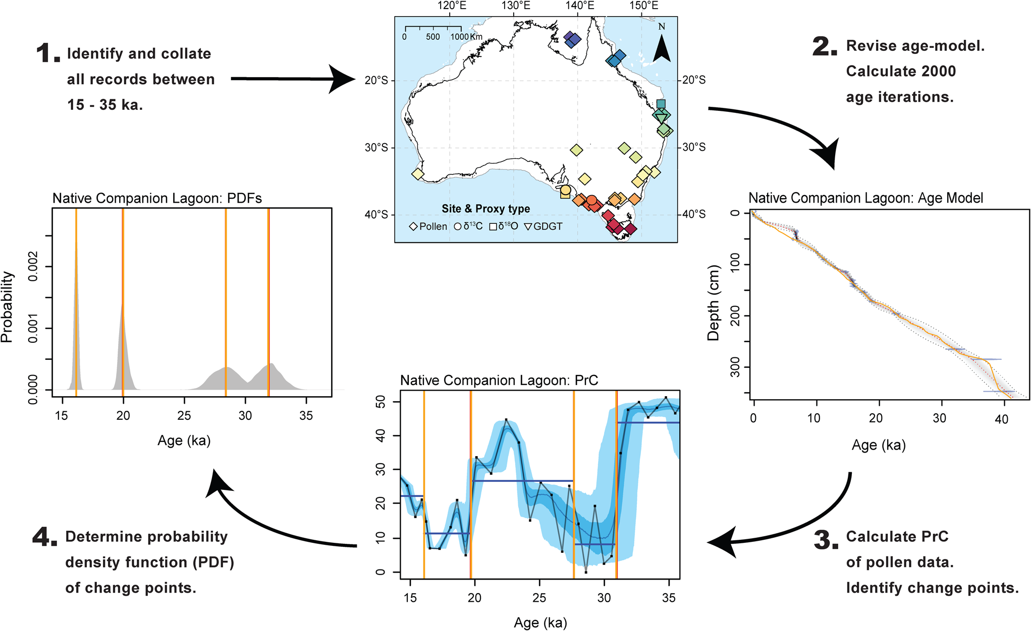
For each record ensemble, the frequency distribution of change points of each ensemble member was compiled and used to calculate the probabilistic age distribution of the timing of change. A probability density function (PDF) was derived for each change point, in all records, along with the weighted average and median values for each PDF. The height of individual peaks within the PDF indicates the probability of the statistically significant change point occurring. The width of the PDF is derived from the 2000 age ensembles and represents the associated age uncertainty for each change point. A visual demonstration of the methodological workflow undertaken in this study is presented in Figure 2.
Schematic of the analytical process used in this synthesis. Step 1: Records were identified and collated (see Table 1 and Figure 1). Step 2: An updated Bayesian age model was determined for each record using Bacon (Blaauw and Christen, Reference Blaauw and Christen2011) and the SH20 calibration curve for radiocarbon dates. 2000 age iterations were extracted from each age model. New age models were compared to original age-model, plotted as an orange line on age-model plot. Step 3: A Principal Curve was applied to compositional data (e.g., pollen spectra) to reduce the data to a single curve. Data for each record [pollen Principal Curves, δ13C, δ18O, and Branched glycerol dialkyl glycerol tetra-ethers (GDGTs)] was then plotted using the weighted mean age from the updated age model (black line). Individual proxy samples are indicated by black squares. Proxy data were plotted using the 2000 age iterations extracted in step 2 (blue shading; 95% and 68% CI). Change point analysis was conducted on each record to determine the timing of changes in the mean of proxy data. Step 4: Identified change points were extracted and each plotted as a Probability Distribution Function. The probability of change (height of peak) results from the likelihood of a change occurring at that time. The uncertainty associated with the timing of change (width of distribution) results from the spread of age iterations determined in step 2. This process was repeated for each identified site. Sites that met the broad criteria were incorporated into further analysis. (For interpretation of the references to color in this figure legend, the reader is referred to the web version of this article.)

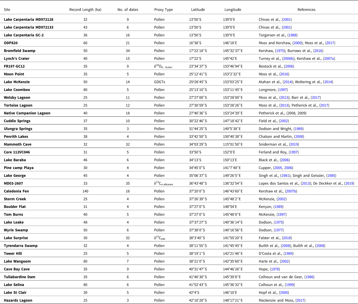
Locations of continuous palaeoclimate and palaeoenvironmental records identified from across Australia covering the last glacial stage (35–15 ka) and included in this synthesis.

Individual change points determined from each record were examined in further detail to identify the direction of the proxy signal and potential climate drivers of each change point. Pollen records are interpreted as responding, in part, to changes in regional climate (primarily mean annual air temperature (MAAT) and change in rainfall amount and seasonality). However, atmospheric CO2 (Prentice et al., Reference Prentice, Cleator, Huang, Harrison and Roulstone2017), site-specific factors, disturbance (i.e., fire), and human modification are also potential contributors to the observed changes (Bond et al,, Reference Bond, Woodward and Midgley2005; Higgins and Scheiter, Reference Higgins and Scheiter2012; Bakker et al., Reference Bakker, Gill, Johnson, Vera, Sandom, Asner and Svenning2016). The primary climate driver of individual pollen records is likely to vary regionally, with the relative influence of changes in MAAT or hydrology difficult to quantify. The δ13C records are also suggested to be a record of catchment vegetation, however with a strong hydrological climate component (Lopes dos Santos et al., Reference Lopes dos Santos, Wilkins, De Deckker and Schouten2012; Falster et al., Reference Falster, Tyler, Grant, Tibby, Turney, Löhr, Jacobsen and Kershaw2018). The δ18O record reflects variation in sea level, sea-surface temperatures and surface–ocean circulation patterns (Bostock et al., Reference Bostock, Opdyke, Gagan, Kiss and Fifield2006), while the GDGT record is primarily interpreted as a record of mean annual temperature (Woltering et al., Reference Woltering, Atahan, Grice, Heijnis, Taffs and Dodson2014).
Changes in biological productivity were converted to simplified climate indices to facilitate inter-site and multi-proxy comparisons. A change point indicating a decline in biological productivity (i.e., from arboreal to grass taxa) is suggested to represent a distinct shift to cooler climates in conjunction with a decrease in available moisture and/or low atmospheric CO2 (herein referred to as a decreasing change point). A change point indicating an increase in biological productivity (i.e., from grass to arboreal taxa) is suggested to represent a distinct shift to warmer climates in conjunction with an increase in available moisture and/or increase in CO2 (herein referred to as an increasing change point). These simplified indices used for assigning climatic changes do not assess the magnitude of changing conditions associated with individual change points and are unlikely to always represent the full range of variability within each dataset. However, the aim of this study, to determine the timing of broad scale regional climate changes in existing palaeoenvironmental records, and the likelihood of synchronous climate changes between those records, dictates the need for a simplified approach to each individual dataset.
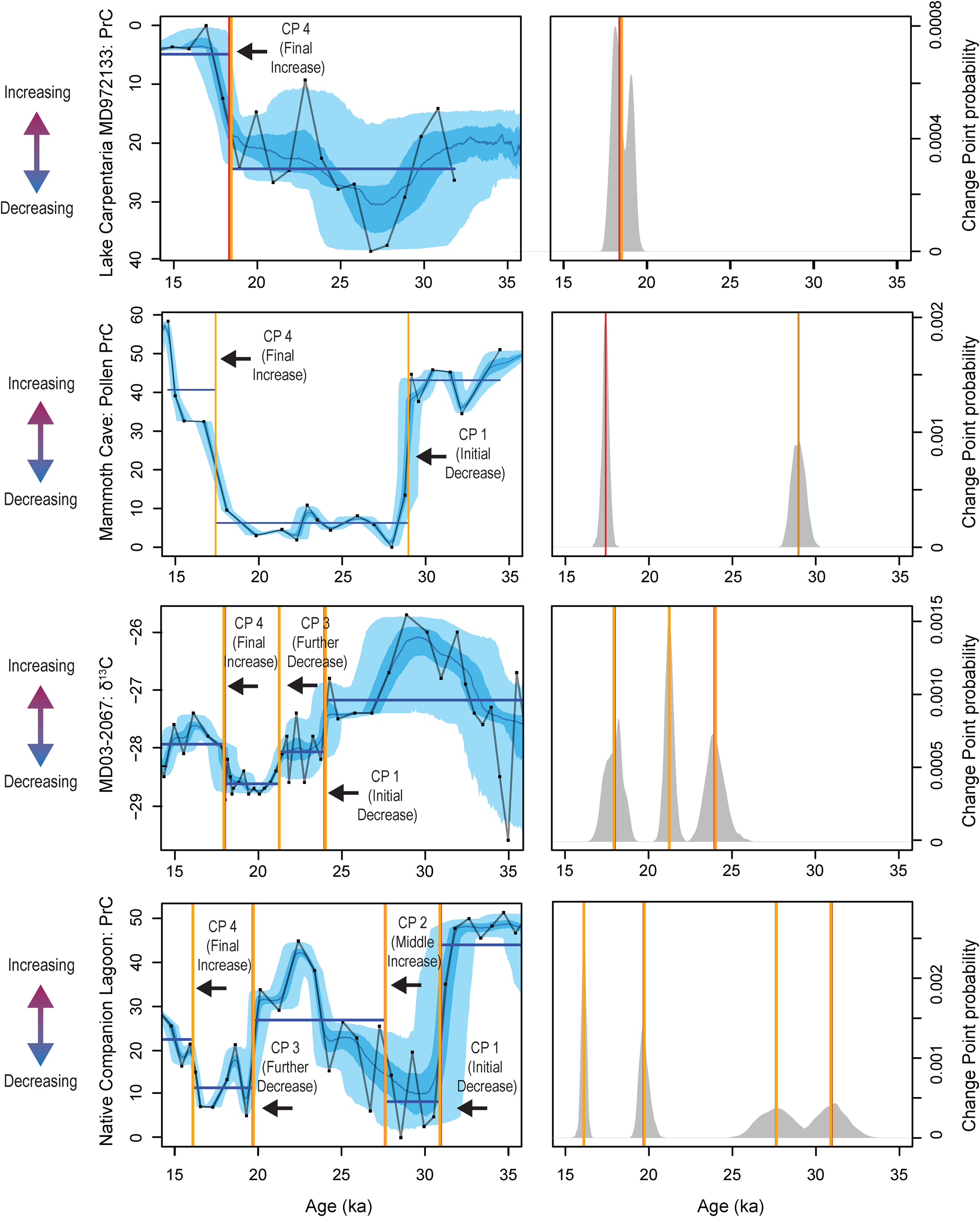
Using the change point information from all records, four periods of change were identified, although not all change points are identified in each individual record: (1) An initial shift to decreasing climate conditions if the records preserved evidence of warmer and/or wetter conditions after 35 ka, before a transition to decreasing climate conditions. (2) A middle change point to increasing climate conditions if a record displayed evidence of a change to increasing climate conditions preceding a decrease in climate conditions. (3) A shift to further decreasing climate conditions if a record displayed a second change point from depressed climate conditions to further decreasing climate conditions, or from increased climate conditions to decreasing climate conditions after an initial change point. If a record displayed evidence of experiencing depressed climate conditions prior to 35 ka (as in Core FR0197) or a record began after 30 ka and already suggested depressed conditions (as in Tortoise Lagoon), a change point to further decreasing conditions was also considered a further change. (4) A transition to increasing climate conditions if a change was categorised as a final transition to increasing climate conditions without a further decrease in climate conditions prior to 15 ka (Fig. 3).
Examples of the different change points identified in the 38 records analysed. (1) Record exhibiting a single change point. (2) Record exhibiting two change points. (3) Record exhibiting three change points. (4) Record exhibiting four change points between 35–15 ka. Change points denoted by vertical lines (orange represents weighted mean of 2000 age-depth model iterations; red represents median of 2000 age-depth model iterations). Light blue shade represents 95% of age-depth vs. proxy relationships, darker blue shading represents 68% of age-depth vs. proxy relationships. Y axis is orientated so that up indicates an increase in biological activity, temperature, or rainfall and down represents a decrease in biological activity, temperature, or rainfall as indicated by coloured arrows. Black line and squares represent proxy data plotted on weighted mean of 2000 age-depth model iterations. See Figure 1 for locations. See Supplementary Materials for change points identified from all records. (For interpretation of the references to color in this figure legend, the reader is referred to the web version of this article.)

RESULTS
Sites included in this synthesis are listed in Table 1. During the age-depth modelling process, sites that did not meet the criteria of encompassing ≥10,000 years between 35–15 ka, or with obvious depositional hiatuses, were excluded from further analysis (Supplementary Fig. 1). The length of individual sedimentary records and number radiocarbon dates are shown in Table 1. The length of records is variable; however, 37 records cover the entire period from 25–15 ka and 36 from 29–25 ka. The number of records extending beyond 30 ka is fewer, and only 15 records that extended beyond 35 ka were identified. The location of all 37 records included in the synthesis are shown in Figure 1. The total number of radiometric ages obtained from the original published records and used in this study was 413 (ranging from 0–47.6 ka). The number of individual radiometric ages from each record varied between 3 and 35 (median = 8).
The number of change points identified was variable across records. A single change point was identified in 18 records, two change points in 14 records, three change points in one record, and four change points in three records. Full details of individual records (see references listed in Table 1) and identified change points are available in the supplementary materials (Supplementary Figs. 3a–ak).
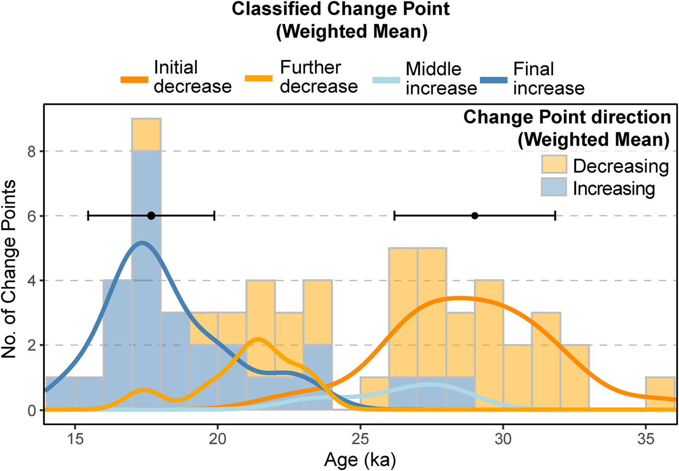
A total of 27 records display evidence for at least one change point identified as decreasing climate conditions (i.e., shift to cooler climates in association with decreased moisture and/or atmospheric CO2), with these change points occurring from 35.6–17.4 ka (Fig. 3, Supplementary Figs. 3a–ak). Frequency distribution of the timing of decreasing change points indicated that the greatest proportion of changes occurred between 26–31 ka (n = 19) (Fig. 4). The remaining nine records do not include a change point identified as decreasing climate conditions. These nine records display evidence of experiencing cool and/or dry conditions prior to 35 ka, or when the proxy record commenced. A total of 28 records display evidence of at least one change point identified as increasing climate conditions (i.e., shifts to warmer climates in association with increased moisture and/or CO2), with these change points occurring between 28.1–14.6 ka (Fig. 3, Supplementary Figs. 3a – ak). Frequency distribution of the timing of increasing change indicates that the greatest proportion of change points occurred between 21–15 ka (n = 21) (Fig. 4). The remaining twelve records do not record a change to increasing warm and/or wet conditions prior to 15 ka and display evidence for the continuation of cool and/or dry climate conditions after 15 ka (Supplementary Figs. 3a–ak).
Frequency distribution of the weighted mean of all significant change points identified in all 38 analysed records. Shading denotes the simplified climate indices assigned to each significant change point as either a decrease in biological activity, temperature, or rainfall (orange) or an increase in biological activity, temperature, or rainfall (blue). Coloured lines indicate change points identified as the initial onset of decreasing climate conditions (i.e., shift to cooler climates in association with decreased moisture and/or atmospheric CO2) (dark orange line), further decrease in climate conditions (light orange line), a middle change to increasing climate conditions (i.e., shift to warmer climates in association with increased moisture and/or atmospheric CO2) (light blue line) and a final increase or termination of extreme conditions (dark blue line). (For interpretation of the references to color in this figure legend, the reader is referred to the web version of this article.)

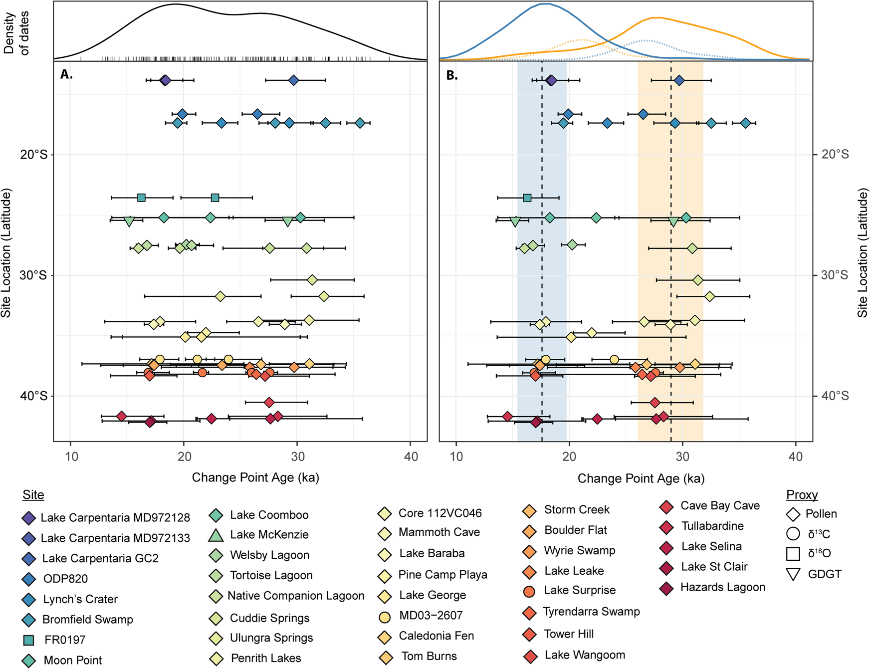
Compilation of identified change points for each site. Weighted mean timing of change points is indicated by coloured symbols. Age uncertainty (95% confidence interval), determined from the ensemble of 2000 age-depth models, associated with each change point is indicated by error bars. Sites are plotted along a latitudinal gradient. (A) All change points identified for each site. (B) Only change points identified and determined as representing the onset of extreme conditions and change decreasing climate indicators (including temperature, precipitation, and CO2) (mean = dashed orange line, SD = shaded orange bar) and the termination of extreme conditions representing increasing climate indicators (including temperature, precipitation, and CO2) (mean = dashed blue line, SD = shaded blue bar). Density of dates curves above panels A and B are kernel density plots of A. Kernel density estimate of both mean and uncertainty of timing of all identified change points derived from the ensemble of 2000 age-depth models and B Kernel density estimate of both mean and uncertainty of timing of change points identified as the onset of extreme conditions (orange line), termination of extreme conditions (blue line) derived from the ensemble of 2000 age-depth models. Change points not assigned to either the onset of termination of extreme conditions are shown by dashed lines. (For interpretation of the references to color in this figure legend, the reader is referred to the web version of this article.)

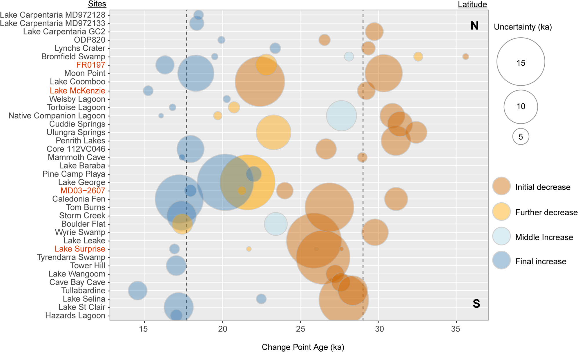
Change points categorised as representing an initial decreasing shift in climate conditions occur at 28.6 ± 2.8 ka (n = 25) (median and one standard deviation of all mean change points). Change points characterised as a middle increasing climate change occur at 26.8 ± 2.1 ka (n = 4). Change points categorised as a further shift to decreasing climate conditions occur at 21.4 ± 1.8 ka (n = 8). Change points categorised as representing a final increasing shift in climate conditions occur at 17.7 ± 2.2 ka (n = 24) (Figs. 4 and 5).
DISCUSSION
An extended period of extreme conditions in Australia
The frequency distribution of the change point analysis conducted on all 37 analysed records indicates two main periods of change, between 30–26 ka, and 20–16 ka (Fig. 4). The compilation of change point analyses indicates consistent timing of change points early in the last glacial period at 28.6 ± 2.8 ka (Figs. 4, 5, and 6). This timing is evident across all climate regions sampled and occurs in 25 of the 27 records that cover the entire 35–15 ka period, suggesting that this change point signal is robust and widespread (Fig. 5). Similarly, a widespread consistent timing of change points occurs late in the last glacial period at 17.7 ± 2.2 ka (Figs. 4 and 5). This change point was recorded in 24 of the 37 records analysed and occurs in all climate regions sampled.
The primary focus of our research is to address the timing of change associated with the extreme conditions of the last glacial stage across Australia, and in order to do so it was necessary to reduce the datasets to simple indices—namely increasing or decreasing indicators (including temperature, rainfall, and CO2). Whilst undoubtedly subject to uncertainty, and requiring of more detailed site-specific consideration, we believe these interpretations provide a useful first-order indicator of the nature of broad changes across the continent. On this basis, analysis of the proposed climatic signal from individual change points from each record show that 88% of change points that occur prior to 26 ka indicate a change to decreasing climate conditions (Figs. 4 and 6). Similarly, of the 28 change points recorded after 21 ka, 79% indicate a change to increasing climate conditions (Figs. 4 and 6). The widespread transition to decreasing climate conditions at 28.6 (± 2.8) ka, and then the subsequent shift towards increasing climate conditions at 17.7 (± 2.2) ka provides objective bracketing for a period of environmental change, consistent with an extended period of cooler and probably more arid climate conditions.
Probability density functions for all sites (coloured lines) and summed probability of (a) all change points, (b) all change points identified as representing a change to decreasing climate indicators (including temperature, precipitation, and CO2), and (c) all change points identified as representing a change to increasing climate indicators (including temperature, precipitation, and CO2). (For interpretation of the references to color in this figure legend, the reader is referred to the web version of this article.)

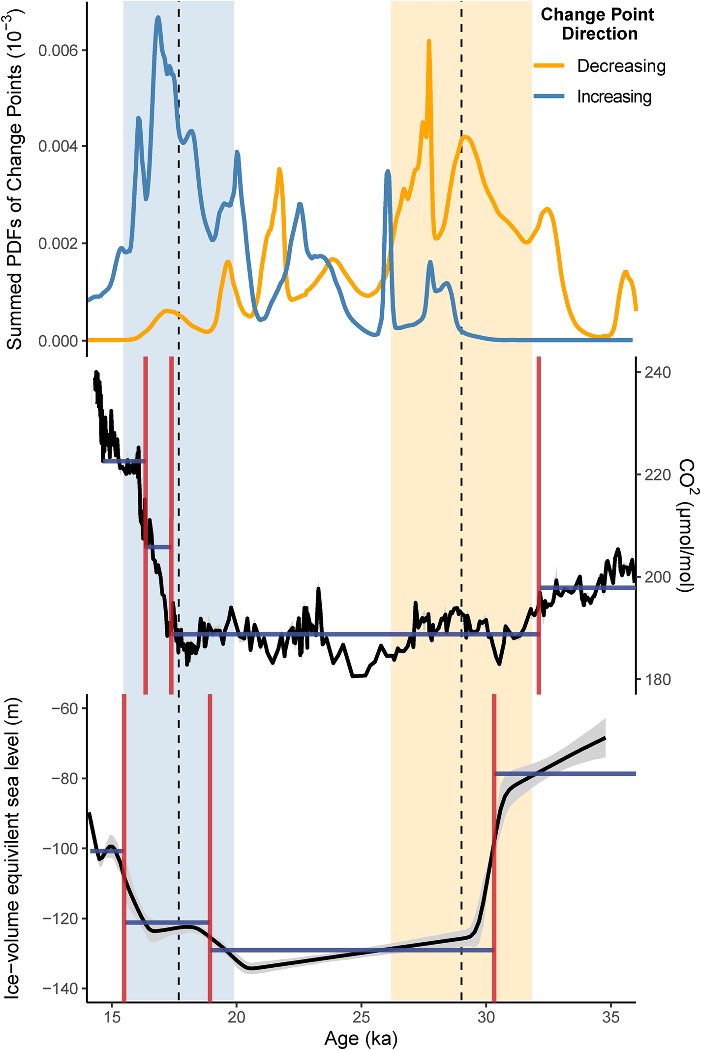
The consistent timing of a change point at 28.6 ± 2.8 ka (shaded orange bar, Figs. 5 and 7) is coincident with the timing of a rapid fall in global sea level (Fig. 7) (Lambeck et al., Reference Lambeck, Rouby, Purcell, Sun and Sambridge2014). Sea levels dropped by ~40 m between ca. 31–29 ka (Lambeck et al., Reference Lambeck, Rouby, Purcell, Sun and Sambridge2014; Yokoyama et al., Reference Yokoyama, Esat, Thompson, Thomas, Webster, Miyairi and Sawada2018). The sharp drop in sea level would have increased the area of the Australian continent, increasing continentality and changing synoptic atmospheric and ocean circulation patterns, leading to changes in regional climates. The timing of this change point corresponds to a modest decline in atmospheric CO2 concentrations of ca. 10 ppm at 27.2 ka (Fig. 7), perhaps indicating that CO2 concentrations were not the primary driver of the vegetation changes identified here. However, the sustained low atmospheric CO2 concentrations during this period may have influenced competitive outcomes, particularly between woody and herbaceous plants, and this may have made vegetation communities more susceptible to small changes in climatic conditions (Cowling and Sykes, Reference Cowling and Sykes1999; Williams et al., Reference Williams, Webb, Shurman and Bartlein2000; Vicente-Serrano et al., Reference Vicente-Serrano, Gouveia, Camarero, Beguería, Trigo, López-Moreno and Azorín-Molina2013) (Fig. 7). A change in climate conditions and/or vegetation cover is indicated at this time from discontinuous geomorphic records, with an increase in dune field activity and dust transport evident after ca. 30 ka (Fitzsimmons et al., Reference Fitzsimmons, Cohen, Hesse, Jansen, Nanson, May and Barrows2013; Hesse, Reference Hesse2016). The timing of these widespread environmental changes in Australia is in agreement with palaeoclimate records from New Zealand which record reductions in arboreal vegetation, lowering of the tree line, and widespread glacial conditions from 28 ka (Hellstrom et al., Reference Hellstrom, McCulloch and Stone1998; Suggate and Almond, Reference Suggate and Almond2005; Alloway et al., Reference Alloway, Lowe, Barrell, Newnham, Almond, Augustinus, Bertler, Carter, Litchfield, McGlone, Shulmeister, Vandergoes and Williams2007; Newnham et al., Reference Newnham, Vandergoes, Hendy, Lowe and Preusser2007; Barrows et al., Reference Barrows, Almond, Rose, Keith Fifield, Mills and Tims2013; Vandergoes et al., Reference Vandergoes, Newnham, Denton, Blaauw and Barrell2013).
(A) Summed probability density function of all change points identified as representing a change to decreasing climate indicators (including temperature, precipitation, and CO2) (orange line) and all change points identified representing a change to increasing climate indicators (including temperature, precipitation, and CO2). (B) Compilation of ice core atmospheric CO2 measurements (ppm) for the period 35–15 ka (Köhler et al., Reference Köhler, Nehrbass-Ahles, Schmitt, Stocker and Fischer2017). (C) Ice volume equivalent sea level (m) (black line) and 95% probability limiting values (grey shading) (Lambeck et al., Reference Lambeck, Rouby, Purcell, Sun and Sambridge2014). Vertical shaded lines indicate the mean and standard deviation of change points identified as representing the onset of extreme conditions (orange) and termination of extreme conditions (blue). (For interpretation of the references to color in this figure legend, the reader is referred to the web version of this article.)

Change points identified and determined as representing an initial change to decreasing climate indicators (including temperature, precipitation, and CO2), a further decrease in climate indicators, a middle shift to increasing climate indicators and a final increase in climate indicators (including temperature, precipitation, and CO2). Size of circle represents the age uncertainty (95% confidence interval), determined from the ensemble of 2000 age-depth models, associated with each change point. Individual records are ordered by latitude from north (13°S) to south (42°S). Non-pollen records are indicated in red text.

The transition out of the extreme climate conditions associated with the last glacial stage and towards the Holocene at 17.7 ± 2.2 ka (shaded blue bar, Figs. 5 and 7), occurring during the deglacial period, correspond to rises in sea level between 20.5–16.6 ka and a substantial increase in global CO2 concentrations beginning at 17.2 ka. The relative importance of different influences on the vegetation communities is difficult to assess across such a broad geographical range, from both monsoonal northern and temperate southern regions. Vegetation records north of 20°S predominantly retain arboreal or woody vegetation cover during the last glacial stage, while vegetation records south of 30°S largely display a shift to grass and herb dominated taxa during this period. The climate forcing required to initiate a change between tree-dominated biomes may be smaller than that required to initiate recovery and recolonization of woody vegetation. The precipitation and temperature increases required to transition from grass and herb vegetation to woody or arboreal vegetation are likely compounded by low atmospheric CO2 levels, increasing the advantage of some functional plant types, while reducing the resilience of other vegetation communities. Many records display additional and, in some cases, increasingly large changes in vegetation or climate leading into and during the Holocene (e.g., records from tropical north Queensland, Bromfield Swamp, and Lynch's Crater), however this later transition is beyond the scope of this paper.
Millennial scale variability
Between the two main periods of change identified in the frequency distribution, a further 12 change points are identified (Figs. 4, 5 and 6) in nine different records. These change points indicate a variable climate between 28.6–17.7 ka at each of these sites. The climatic implications of the 12 identified change points during this time are not consistent, with eight of the change points indicating a change to decreasing climate indicators (including temperature, rainfall, and CO2), and four indicating a change to increasing climate indicators (including temperature, rainfall and CO2). The occurrence of multiple change points during this period highlights the variable nature of climate and environmental conditions across Australia during the last glacial stage and underscores the challenges associated with interpretation of simplified climate indices.
Of these identified change points, three records indicate a two-step change from decreasing climate conditions to further decreased conditions (Bromfield Swamp, Ulungra Springs, and Murray Canyons). A further three records register a change point towards decreasing conditions after 25 ka (Tortoise Lagoon, Lake George, and Boulder Flat). These records do not extend beyond 30 ka and demonstrate relatively cool and/or dry conditions when each record began. The FR0197 G. ruber δ 18O record indicates lower sea levels, potentially coupled with different surface–ocean circulation patterns and/or cool SST, throughout the period 35–25 ka, before a shift at 23 ± 3.5 ka.
The remaining two records (Native Companion Lagoon and Lake Surprise) suggest the extended period of uniform climate conditions was interrupted by a period of warmer and/or wetter conditions. Neither the timing of the onset or the termination of this period, nor the duration of this warmer and/or wetter period, is the same in these records. The limited number of records indicating the presence of a millennial scale change during an otherwise extended period of relative climate stability may indicate this phenomenon was not widespread. However, the limited identification of this millennial scale change may be a function of the number of sufficiently resolved records able to detect short-term fluctuations in climate during this period. Many of the proxy records analysed here have too coarse a temporal resolution to reliably identify millennial scale variability. The presence of this signal in records from the east coast (Native Companion Lagoon) and southwest Victoria (Lake Surprise) may suggest any millennial-scale cycles in this period (need they be synchronous or separate events) may have been geographically widespread, at least on the eastern half of the continent. This period of altered climatic conditions may have been insufficient to drive substantial changes in vegetation composition in various ecological settings. In addition, the resilience of various vegetation communities under the low atmospheric CO2 conditions during the last glacial stage may have restricted a rapid response of ecosystems to brief periods of increased temperature and/or moisture availability.
Whilst a period of increased temperature and/or moisture availability displayed in Native Companion Lagoon and Lake Surprise is not manifest in any other records analysed here, an additional six records have a second change point to decreasing climate conditions (including temperature, rainfall, and CO2). These change points can be characterised either as a shift from already depressed climate conditions to further decreasing climate conditions (Ulingra Springs and MD03-2607), further reduction in sea level (FR0197), or a change to decreasing climate conditions in records that do not extend from 35–30 ka (Tortoise Lagoon and Lake George). Combined with the two records that record a shift to decreasing climate conditions at the termination of a period of increased temperature and/or moisture availability (Native Companion Lagoon and Lake Surprise), a change to decreasing climate conditions at 21.4 ± 1.8 ka in eight records is indicated during the originally defined global LGM (Yokoyama et al., Reference Yokoyama, Lambeck, De Deckker, Johnston and Fifield2000). The occurrence of a change point toward further decreasing temperature, moisture availability, or CO2 in this subset of records, coincident with the timing of the absolute global sea-level minimum, suggests that this period was potentially represented by a further reduction in either effective precipitation or temperature that culminated in maximum glaciation in Australia (Barrows et al., Reference Barrows, Stone, Fifield and Cresswell2002).
Climate implications
The records compiled for this multi-site comparison primarily reflect vegetation change and therefore represent environmental responses to climate change (Fig. 1, Table 1). As such, assigning definitive climate drivers to such changes is difficult. However, the consistent timing of changes within the pollen records indicates that, although vegetation changes are susceptible to multiple drivers and time-transgressive responses, there is likely an overarching first-order climatic driver operating on most records analysed here (Figs. 5, 6, and 8). The clear climatic signal evident in the large number of pollen records analysed may be indicative of the extreme and substantial climatic changes during this period, as well as the potential sensitivity of different Australian ecosystems to climate forcing. Whilst individual pollen records may not record a primary climate signal, the compilation of several records across regional spatial scales can increase the confidence in the likelihood of climate as a primary driver. The large number of pollen records that demonstrate the same signal, across a broad spatial range, enables regional interpretations of climate to be made.
Future research directions
The work presented here provides evidence for synchronous, widespread environmental change across Australia associated with both the onset and termination of extreme climate conditions during the LGM (Fig. 7). To provide more detailed information on the potential widespread nature of the changes identified here requires the development of more continuous palaeoclimate records from under-represented climate regions. The distribution of continuous terrestrial archives in Australia is largely restricted to the eastern and southern regions of the continent (Fig. 1). The potential for developing palaeoclimate records that are continuous through the last glacial period from the western, northwestern, and centre of the continent is more limited. However, recent work from some of these regions has identified continuous proxy records that extend to this time period (Field et al., Reference Field, Tyler, Gadd, Moss, McGowan and Marx2018; Rowe et al., Reference Rowe, Wurster, Zwart, Brand, Hutley, Levchenko and Bird2020). Incorporation of discontinuous geomorphic archives of palaeoclimate into future syntheses, and improved climatic interpretations of such records, would broaden the spatial coverage to regions where preservation of continuous terrestrial archives is incomplete or less dense.
The proxy resolution and age uncertainty of many records analysed in this compilation make it difficult to provide a more precise timing of climate changes associated with the last glacial stage, including the onset and termination of these changes. There are few records currently available that allow sub-millennial scale changes, precise timing of regional variations, and external climate drivers to be accurately determined. In order to more precisely identify the timing of key environmental events and their relationships to climate change, high resolution proxy data coupled with independently and densely dated chronologies are required. The continued incorporation of high-resolution geochemical records from micro X-ray fluorescence analysis (μXRF) core scanning could provide an important additional proxy dataset that can be compared to more traditional palynological datasets and substantially improve the resolution of records of environmental change during the last glacial stage. The methods employed here incorporate the chronological uncertainty associated with age-depth model development and interpolation between dated depths, however no assessment is made of the quality of the radiometric dates used. Identification of anomalous radiometric ages and accurate quantification of individual age determinations requires an increase in the density of dated layers (Blaauw et al., Reference Blaauw, Christen, Bennett and Reimer2018) and dating of multiple sediment fractions (Martin et al., Reference Martin, Goff, Jacobsen and Mooney2019; Thomas et al., Reference Thomas, Turney, Hogg, Williams and Fogwill2019). The presence of sedimentary hiatuses in records used in this compilation may currently be masked by the limited number of radiometric ages analysed from some sites (Supplementary Fig. 2). Verification of ages by a form of independent age control (e.g., optically stimulated luminescence or uranium-thorium methods) would provide additional chronological certainty. Enhanced application of rigorous chronological modelling methodologies and accounting for inherent age uncertainties will further enhance the capacity for inter-site comparisons and regional syntheses (Blaauw et al., Reference Blaauw, Christen, Bennett and Reimer2018; Blaauw et al., 2019, Blaauw et al. Reference Blaauw, Christen and Aquino-López2020).
Improvement of proxy resolution and reduction of age-uncertainty will further increase the potential for more robust statistical analysis and record comparison. Here, we used a mean change point analysis, from the changepoints package in R, to attempt to identify the timing of the most extreme conditions during the last glacial stage from proxy records of varying temporal resolution. Implementation of a mean change point method was chosen to provide a simple and repeatable measure of timing of changes within datasets incorporated in this synthesis, which vary strongly in their temporal resolution and in the ‘noisiness’ of their proxy signals. However, the mean change point approach assumes that all time series can be adequately represented by a series of n segments, each with a stationary mean and randomly fluctuating noise components. In fact, time series data can be more complex, with linear trends, changes in trend and red noise all common features of palaeoclimate timeseries (Beaulieu and Killick, Reference Beaulieu and Killick2018). This work is a first step in the use of change point analysis to compare and synthesise multiple palaeoenvironmental records of varying temporal and proxy resolution. Exploration of change point methodologies with greater complexity of analysis afforded by newly developed software, such as those implemented in the EnvCpt change point package (Beaulieu and Killick, Reference Beaulieu and Killick2018), will continue to improve conclusions of spatial and temporal synthesis.
Palaeoclimate reconstructions derived from biological and geomorphological proxy evidence may be influenced by a variety of additional factors (e.g., atmospheric CO2 variations and human modification) and display time-transgressive responses to climate forcing. An accurate understanding of the magnitude of past climate changes and their influence on local environmental conditions requires a network of quantitative precipitation and temperature reconstructions, based on organic and/or isotope geochemical tracers (e.g., GDGTs, alkenone palaeothermometry, oxygen and hydrogen isotopes) across a variety of climate regions. Validation of interpreted changes via independent estimates of both temperature and precipitation across both terrestrial and oceanic records would further allow the magnitude of changes and interactions between climate variables to be disentangled. Comparison of these independent, quantitative hydrological and temperature records with records of vegetation change would reduce the ambiguity of the role of precipitation, temperature, pCO2, or disturbance in driving vegetation transitions. In addition, incorporation of quantitative local climate reconstructions would provide a foundation on which to test how variations in atmospheric CO2 influence vegetation resilience and response to climate changes.
Supplementary Material
The supplementary material for this article can be found at https://doi.org/10.1017/qua.2021.16
Acknowledgments
We would like to thank the various researchers who have contributed datasets for this compilation. We thank Merna McKenzie for providing data (on floppy disk) to be included in this synthesis, and Martin Ankor helping to extract the data from disk and DOS Tilia format. All data used in this synthesis will be made publicly available on the Neotoma database. We thank all members of the SHeMax working group who contributed to discussions during workshops in Auckland and North Stradbroke Island.
Financial Support
This research was supported by Australian Research Council (ARC) Centre of Excellence for Australian Biodiversity and Heritage (CABAH) and ARC DP150103875. Haidee Cadd was supported by a CABAH Internship for Women during part of this work. Annika Herbert is supported by funding from the DSI-NRF Centre of Excellence for Palaeosciences, South Africa.