

1. Introduction
The interactions between a compliant wall and turbulent or laminar boundary layer have been investigated extensively for over 60 years. Most of the interest has been stimulated by bio-inspired attempts to reduce the skin friction, starting from observations by Kramer (Reference Kramer1957, Reference Kramer1962), and followed by experiments by, e.g. Fisher & Blick (Reference Fisher and Blick1966), Blick & Walters (Reference Blick and Walters1968), Choi et al. (Reference Choi, Yang, Clayton, Glover, Atlar, Semenov and Kulik1997), Harris & Lissaman (Reference Harris and Lissaman1969) and McMichael, Klebanoff & Mease (Reference McMichael, Klebanoff, Mease and Hough1980). These efforts have not led to conclusive answers. Theoretical work by Benjamin (Reference Benjamin1960, Reference Benjamin1963) and Landahl (Reference Landahl1962) aimed at delaying the transition from laminar to turbulent boundary layers suggests that proper selection of the compliant material properties might the suppress instabilities that trigger the transition. Carpenter & Garrad (Reference Carpenter and Garrad1985, Reference Carpenter and Garrad1986) conclude that these instabilities can be divided into two categories, namely Tollmien–Schlichting (TS) instabilities that occur also over a rigid wall, and flow-induced surface instabilities (FISI) associated with surface deformation. Wind tunnel experiments by Lee, Fisher & Schwarz (Reference Lee, Fisher and Schwarz1993a,Reference Lee, Fisher and Schwarzb) and direct numerical simulation (DNS) by Wang, Yeo & Khoo (Reference Wang, Yeo and Khoo2006) have concluded that the wall compliance could suppress the TS waves, and material damping could reduce the FISI.
Past studies have also shown that interactions between compliant surfaces and turbulent boundary layers involve two coupled aspects, namely the formation of deformation waves, and the impact of these deformations on the flow structure and turbulence in the boundary layer. Early experiments focusing on drag reduction have used very soft compliant materials, i.e. with a flow speed several times higher than the material shear-wave speed. They have revealed the formation of static divergence waves (Hansen & Hunston Reference Hansen and Hunston1974, Reference Hansen and Hunston1983; Gad-el-Hak, Blackwelder & Riley Reference Gad-El-Hak, Blackwelder and Riley1984, Lucey & Carpenter Reference Lucey and Carpenter1992), which are aligned in the spanwise direction, and have a very low phase speed (~0.05U 0, where  $U_0$ is free-stream velocity). Another theoretically observed phenomenon is travelling-wave flutter (TWF), a convective instability associated with the phase difference between the pressure fluctuations and the complaint wall vertical velocity (Gad-el-Hak Reference Gad-El-Hak1986; Carpenter, Davies & Lucey Reference Carpenter, Davies and Lucey2000). It has an advection speed of approximately 0.7U 0, and its amplitude grows in the streamwise direction, but not in time.
Several methods have been used for measuring smaller deformations. Point measurements tracking the displacement of a laser beam reflected from a surface are described by Gad-el-Hak et al. (Reference Gad-El-Hak, Blackwelder and Riley1984) and Hess, Peattie & Schwarz (Reference Hess, Peattie and Schwarz1993). Improvements in resolution to submicron levels have been achieved using a laser Doppler vibrometer (e.g. Castellini, Martarelli & Tomasini Reference Castellini, Martarelli and Tomasini2006; Tabatabai et al. Reference Tabatabai, Oliver, Rohrbaugh and Papadopoulos2013). Two-dimensional deformation maps have been obtained for the first time using holographic interferometry by Lee et al. (Reference Lee, Fisher and Schwarz1993a,Reference Lee, Fisher and Schwarzb). Recording the interferogram on film, their data are not time resolved. Recently, Zhang, Miorini & Katz (Reference Zhang, Miorini and Katz2015) and Zhang et al. (Reference Zhang, Wang, Blake and Katz2017) have introduced a time-resolved system, which simultaneously measures the two-dimensional (2-D) surface deformation using Mach–Zehnder interferometry (MZI), and the 3-D velocity field using tomographic particle image velocimetry. The MZI system, which is used in the present paper and discussed in more detail later, uses a correlation-based fringe enhancement procedure to achieve an uncertainty of approximately 20 nm. Another 2-D surface mapping tool involving direct digital image correlations or a dot tracking algorithm combined with free surface-synthetic schlieren (Moisy, Rabaud & Salsac Reference Moisy, Rabaud and Salsac2009) to measure the displacement of random dot patterns is introduced by Charruault, Greidanus & Westerweel (Reference Charruault, Greidanus and Westerweel2018). This procedure has been subsequently used by Benschop et al. (Reference Benschop, Greidanus, Delfos, Westerweel and Breugem2019) to characterize and model the deformation of compliant walls over surfaces with varying properties. Their findings and model predictions are compared to the present results in §§ 4 and 6 of this paper.
Numerical simulations have also been used to investigate the interaction between the boundary layer turbulence and the compliant surface deformation. In, for example, Endo & Himeno (Reference Endo and Himeno2002), Xu, Rempfer & Lumley (Reference Xu, Rempfer and Lumley2003) and Kim & Choi (Reference Kim and Choi2014) the surface is modelled as a distributed spring–damper system. The latter observe that, for soft materials, large-amplitude quasi-2-D surface waves travel downstream at a phase speed of less than 40 % of the centreline velocity. For stiffer walls, the deformation pattern becomes more complex and travels at 72 % of the centreline velocity. In both cases, there was no drag reduction. Rosti & Brandt (Reference Rosti and Brandt2017) have been the first to perform DNS of turbulent channel flow over a hyper-elastic compliant wall, where the solid is a neo-Hookean material satisfying the incompressible Mooney–Rivlin law (Mooney Reference Mooney1940; Rivlin Reference Rivlin1948). Their Reynolds number is very low (Reτ ~ 180), and the amplitude of the compliant wall deformations is several wall units, resulting in the two-way coupling between the flow and the deformation. Their material properties are related to the flow dynamics using the scaled Young modulus,  $E/\rho U_0^2$, where
 $\rho$ is fluid density. They show that, with decreasing
 $E/\rho U_0^2$, the flow transitions from being streamwise correlated to spanwise correlated. Furthermore, the wall deformations cause a downward shift in the velocity in the log layer and an increase in the slope of the mean velocity profile in the viscous sublayer. These interactions also increase all the Reynolds stresses and modify the structure of the near-wall turbulence. These findings are also discussed and compared to the present experimental data, which are obtained for much higher Reynolds numbers and stiffer walls.
In our above-mentioned previous experimental study of turbulent channel flow over a compliant wall (Zhang et al. Reference Zhang, Miorini and Katz2015, Reference Zhang, Wang, Blake and Katz2017), the deformation amplitude is much smaller than one wall unit, hence it predominantly involves one-way coupling between the flow and deformation. In the present study, the material properties and coating thickness are selected to establish two-way coupling based on theoretical predictions of the response of compliant coatings to pressure perturbations. Examples of relevant models are provided in Duncan (Reference Duncan1986), Chase (Reference Chase1991), and recently in Benschop et al. (Reference Benschop, Greidanus, Delfos, Westerweel and Breugem2019). As discussed in § 2, following our prior work, we start by utilizing the linear one-dimensional model introduced by Chase (Reference Chase1991) to predict the response of a visco-elastic material to pressure perturbation with prescribed amplitude and frequency. The scales of the deformation are selected to achieve two-way coupling and fall within the spatial and temporal resolutions of our instruments, which are described in § 3. Results for the deformation as well as the boundary layer flow and turbulence, which are presented in §§ 4 and 5, indeed confirm that two way coupling occurs, but starts at deformation scales much smaller than expected. Section 6 contains the discussion and conclusions.
2. Design of the compliant surface and experimental conditions
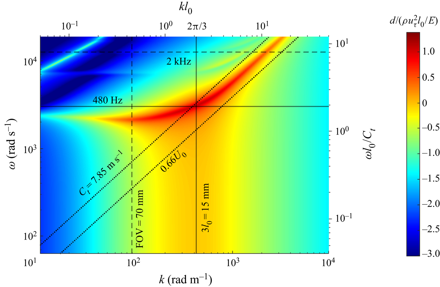
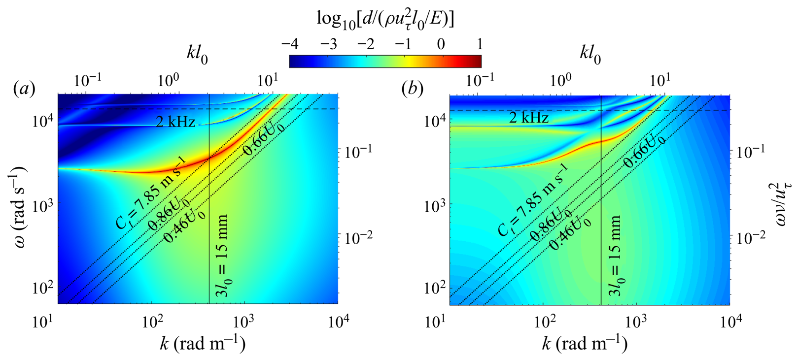
Following Zhang et al. (Reference Zhang, Wang, Blake and Katz2017), a Matlab-based code for calculating the response of visco-elastic material based on the Chase (Reference Chase1991) model has been used for determining the desired material properties, including the Young and shear moduli, loss coefficient and coating thickness. Our objectives have been to (i) have deformation amplitudes of a few wall units, (ii) a range of wavenumbers that falls within a convenient field of view of the imaging systems (~70 mm) and (iii) a peak response frequency of less than 2 kHz allowing full use of the camera resolution. Multiple iterations have led to the selection of a material whose response to pressure excitations with a constant amplitude of  $\rho u_\tau ^2$ (uτ is the friction velocity in turbulent boundary layer) is portrayed in figure 1.
The amplitude of deformation (normalized by  $\mathrm{\rho }u_\tau ^2{l_0}/E$) in response to constant pressure perturbation with an amplitude of
 $\rho u_\tau ^2$, as predicted by the Chase (Reference Chase1991) model.

Here, ω(= 2πf) is the frequency multiplied by 2π, k is wavenumber, l 0 is the thickness of the coating and Ct is the material shear speed, E is the Young modulus, ρ is the fluid density and uτ is the turbulent boundary layer friction velocity as discussed before. The frequency and wavenumber are presented both in dimensional and dimensionless forms, and the amplitude is normalized by  $\rho u_\tau ^2{l_0}/E$. Note that this response assumes a uniform excitation amplitude and constant material properties. Further analysis later in this paper accounts for the variations in properties and pressure fluctuation amplitude with frequency. Based on this prediction, at a free-stream velocity of 6 m s−1, friction velocity of 0.21 m s−1 and E ~ 158 kPa (based on the measurements below), the maximum deformation peak is approximately 24 μm, which is several times larger than the corresponding wall unit (~5 μm). Hence, provided the material is excited at the proper frequency and wavenumber, a two-way coupling of the flow and the deformation should be expected. Furthermore, for a layer thickness of 5 mm, the wavelength of peak response (3l 0) is 15 mm, and the corresponding frequency is 480 Hz. Hence, a field of view of 70 mm × 35 mm2 and an image acquisition rate of 2 kHz should be sufficient to resolve the 2-D surface deformation.
To facilitate characterization of the surface deformation using MZI (Zhang et al. Reference Zhang, Wang, Blake and Katz2017), we have opted to use a silicone-based transparent coating made of polydimethylsiloxane (PDMS). The material properties are then varied/controlled by mixing the PDMS with a silicone gel. The compliant surface is manufactured by mixing Dow Corning Sylgard™ 184 (PDMS) and Sylgard™ 527 (gel), Using a PDMS to gel mass ratio of 1 : 7.5, the data provided by Palchesko et al. (Reference Palchesko, Zhang, Yan and Feinberg2012) suggest that the storage modulus of this material should be around 80 kPa. Samples of this material have been manufactured and then sent to the Naval Surface Warfare Center, Carderock Division, to measure their properties at the relevant range of frequencies (Technical report no. TR180613-02). The complex elastic modulus, E*, as a function of the angular frequency (ω) can be determined using
 \begin{equation}{E^\ast }(\omega) = {E_0}\frac{{\textrm{i}{\omega ^m}\Gamma (1 - m){\textrm{e}^{ - \textrm{i}(1 - m)\pi /2}}}}{{{{[1 + {{(\textrm{i}\omega \tau)}^\alpha }]}^\beta }}} + {E_\infty }\left\{ {1 - \frac{1}{{{{[1 + {{(\textrm{i}\omega \tau)}^\alpha }]}^\beta }}}} \right\},\end{equation}
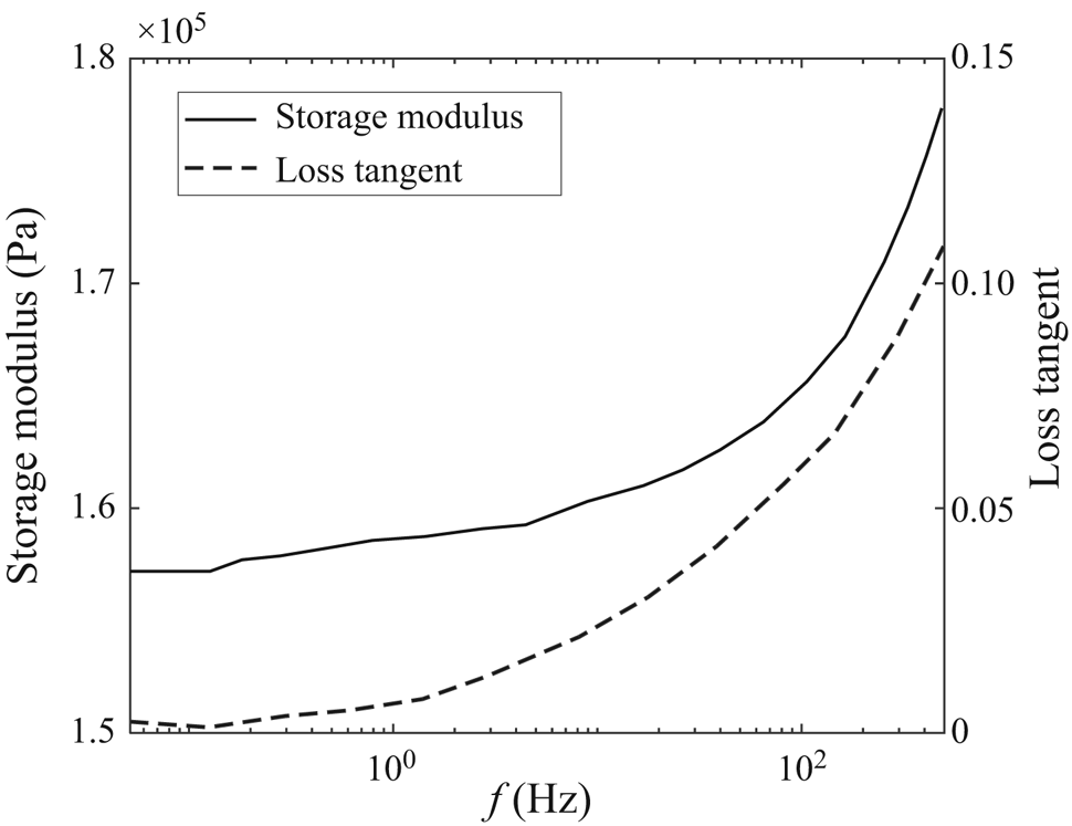
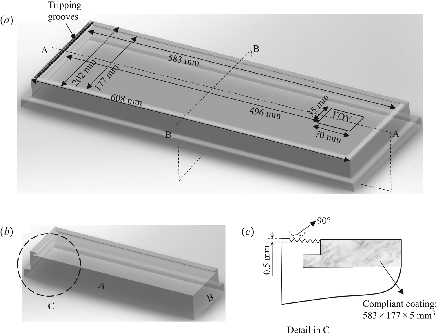
which has six measured temperature-dependent, Havriliak–Negami coefficients, namely E∞, E 0, m, τ, α and β (Hartman, Lee & Lee Reference Hartman, Lee and Lee1994). Based on the measured values (E∞ = 556 kPa, E 0 = 158 kPa, m = 0.0029, τ = 2.57 × 10⁻⁴, α = 0.739, β = 6.54 × 10⁻⁵), the static storage modulus of this material is E 0 = 158 kPa, and the shear speed estimated using  $Ct = \sqrt {E/2(1 + {\nu _p}){\rho _s}} $, is 7.85 m s−1, where νp = 0.4995 is the Poisson ratio and ρs is the density of the compliant material. Figure 2 summarizes the experimental measurements of storage modulus and loss tangent for this material as a function of frequency. This compliant surface is softer than the one described in Zhang et al. (Reference Zhang, Wang, Blake and Katz2017), where the storage modulus is ~1 MPa, and the shear speed is 17 m s−1. A special 5 mm wide moulding chamber, which already contains the acrylic wall of the water tunnel, has been constructed. The mixture is poured into this chamber while it is kept below atmospheric pressure (87.5 kPa) to minimize the formation of bubbles, and then allowed to cure at room temperature (~25 °C). The typical curing time is approximately 48 hours. The dimension of the compliant coating is 583 mm × 177 mm × 5 mm3 in length, width and thickness, respectively. The refractive index of this material measured using a refractometer (Waterproof Digital Refractometer Brix) is 1.406, and its density, as proved by the manufacturer and measured by the Naval Surface Warfare Center, Carderock Division, is approximately 0.855 g cm−3. To hold the compliant surface attached to the water tunnel window, the periphery of the (50.8 mm thick) acrylic window has a 12.7 mm wide overhanging rim and threaded holes (figure 4a,b). We have not used any chemical bonding between the compliant material and the acrylic to prevent potential distortion of MZI images. The current design works effectively for flow speeds up to 7 m s−1, but the compliant coatings have been partially peeled off after one day at 5.9 m s−1, requiring repeated installations. A separate mould with a thickness of 3.14 mm has been used for preparing samples for testing the material properties.
The frequency-dependent storage modulus and loss tangent of the compliant surface measured at T = 25 °C.

3. Test facility and experimental set-up
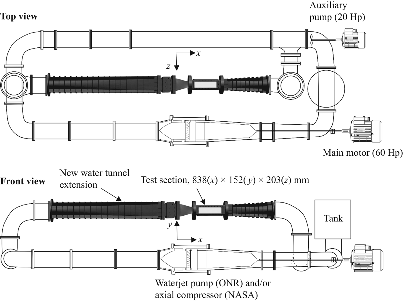
The experiments have been performed in a new water tunnel extension/bypass of the Johns Hopkins University refractive index-matched test facility. A schematic of this water tunnel is presented in figure 3. The working fluid is an aqueous sodium iodide (NaI) solution, whose refractive index (1.4876) is matched with that of acrylic, but not that of the compliant material. The density of the fluid is ρ = 1.86 × 10³ kg m−3 and its dynamic viscosity is ν = 1.1 × 10⁻⁶ m2 s−1. The flow in this system is driven by two pumps. The main driver is either an axial waterjet pump or a replica of an axial compressor connected to a 60 Hp motor. These devices have been the subject for several studies in themselves (Tan et al. Reference Tan, Li, Wilkes, Vagnonii, Miorini and Katz2015; Li, Chen & Katz Reference Li, Chen and Katz2017). Additional power is provided by a 20 Hp auxiliary axial pump. The highlighted new extension consists of a long diffuser, a 406 mm × 348 mm settling chamber containing screens and a honeycomb, a nozzle with an area ratio of 4.6 : 1, a test section with windows on all sides and another diffuser expanding back to original 30.5 cm pipe. The size of the test section is 838 mm × 152 mm × 203 mm3 in the streamwise (x), wall-normal (y) and spanwise (z) directions, respectively. It consists of a stainless steel frame and 50.8 mm thick acrylic windows. The present experiments have been performed at speed ranging between 1.2 and 5.9 m s−1, the latter being well below the maximum level. The 5 mm thick compliant surface is embedded in the bottom window. The boundary layer is tripped upstream of this surface using a series of 5 mm high grooves (figure 4a,c), which are similar to those used in Ling et al. (Reference Ling, Srinivasan, Golovin, McKinley, Tuteja and Katz2016) to establish a fully developed turbulent boundary layer. The velocity and deformation measurements are performed 496 mm downstream of the beginning of the compliant surface and 508 mm downstream of the tripping grooves.
Schematics of the new refractive index-matched water tunnel.

The window containing the compliant coating: (a) a full view of the window, showing the locations of the sample area and the tripping grooves, (b) a section view of the window with planes A and B indicated in (a) and (c) the upstream end (view C) showing the tripping grooves and compliant coating installed.

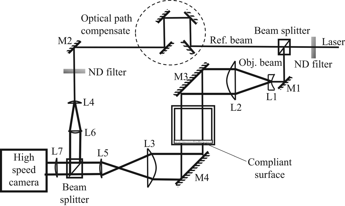
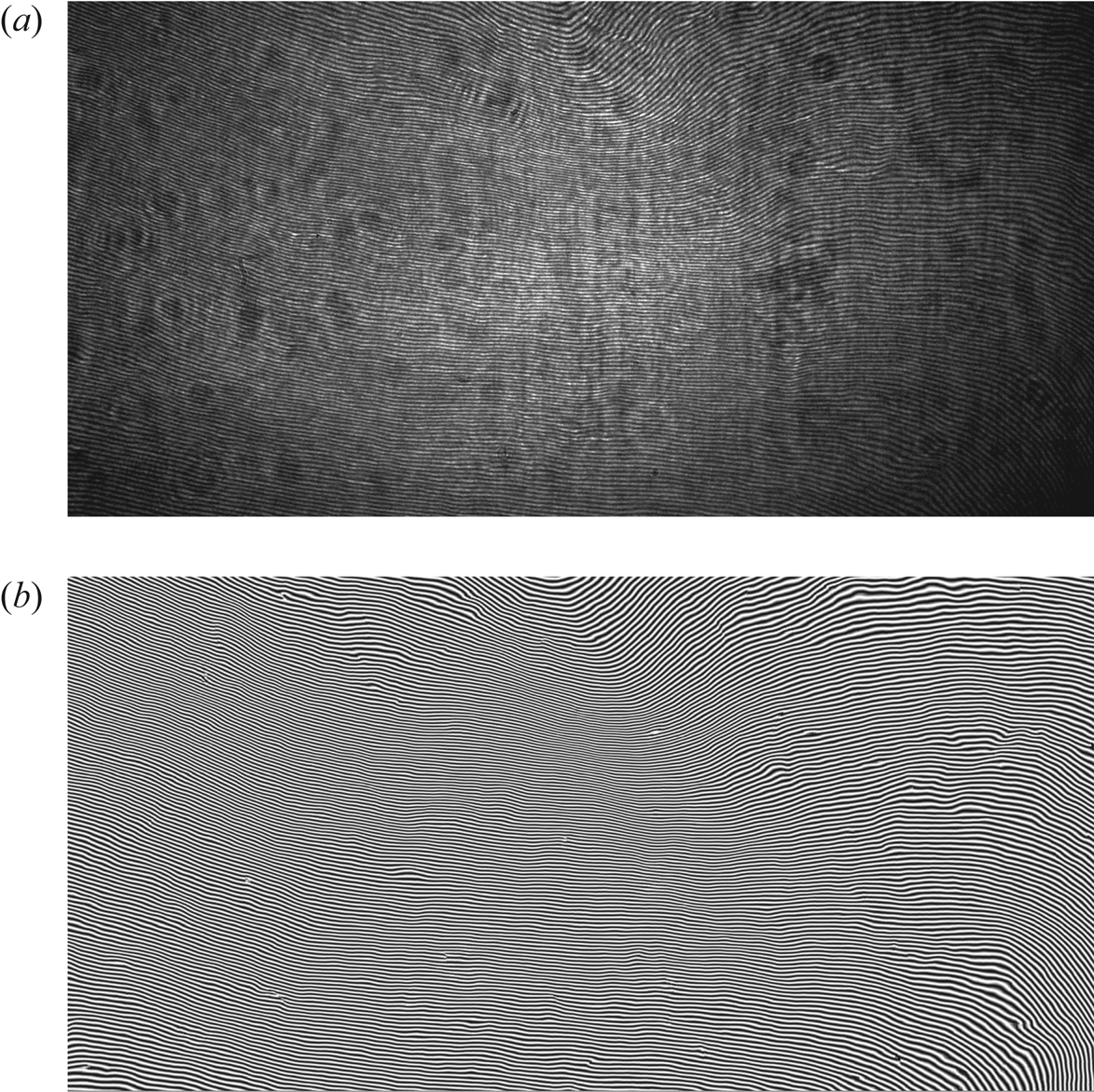
Figure 5 is a sketch of the set-up for measuring the wall deformation using MZI. Details on the data analysis procedures of associated uncertainty are provided in Zhang et al. (Reference Zhang, Miorini and Katz2015). The beam of a high-speed Nd, YLF laser (Photonics model DM60-527) is attenuated by an ND 0.9 filter and then split into reference and object beams. The object beam is expanded to a diameter of approximately 10 cm and directed across the test section and the compliant wall using 20 cm diameter mirrors and lenses. This beam is then reduced to approximately 2 cm and directed to the camera. Using 10 cm diameter lenses and mirrors, the reference beam bypasses the test section and is then combined with the object beam by a non-polarizing beam splitter before illuminating the camera. The optical path lengths of the two beams are matched by varying the path of the reference beam until the interference fringes appear (figure 6a). The 2016 pixel × 1012 pixel interferograms are recorded at 2 kHz by a PCO.dmax camera, resulting in a field of view of 70 mm × 35 mm2 in the x and z directions, respectively. As discussed in Zhang et al. (Reference Zhang, Miorini and Katz2015), the fringes are enhanced using spatial correlation-based filtering, and the phase distributions are measured directly from the enhanced images. In the present data, the typical fringe spacing is 0.35 mm, defining the lateral resolution, but the uncertainty in the wall-normal direction is approximately 20 nm, i.e. ranging between 2.0 % and 0.1 % as the deformation increases from 1 to 20 μm. A total of 7000 fringe patterns are captured for each flow condition, namely at six free-stream velocities of 1.2, 1.9, 3.2, 4.5, 5.3 and 5.9 m s−1.
Set-up of the large field of view Mach–Zehnder Interferometer used for measuring the 2-D surface deformation.

Samples of MZI fringe patterns (U 0 = 3.2 m s−1): (a) raw data and (b) correlation-based enhanced image.

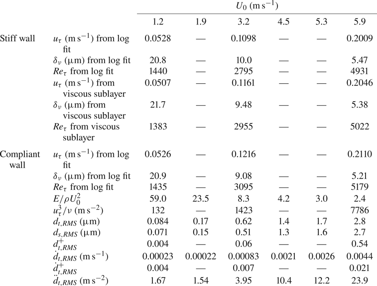
To characterize the boundary layer profile, two-dimensional particle image velocimetry (PIV) measurements have been performed in a central streamwise—wall-normal plane above the compliant wall. The light source is an Nd-YAG laser (532 nm) whose beam is expanded to a 0.5 mm thick laser sheet. The image pairs are recorded using an Imprex ICL-B6640 interline transfer camera that has a 6600 pixel × 4400 pixel array. Using a 105 mm lens and an extension tube, the images are recorded at a magnification of 1.67, resulting in a pixel resolution of 3.3 μm pixel−1. The flow field is seeded globally using 2 μm diameters, silver-coated glass spheres – Potters Industries Conduct-O-Fil® SG02S40 particles. These particles have a density of 4 g cm−3, but owing to their size, are expected to have negligible slip relative to the surrounding flow (Adrian Reference Adrian1991; Grant Reference Grant1997; Melling Reference Melling1997). The delays between exposures, 40, 15 and 8 ms for free-stream speeds of 1.2, 3.2 and 5.9 m s−1, respectively, have been selected to maintain a maximum particle displacement of approximately 12 pixels. For each case, 17 000 pairs of particle images have been recorded to facilitate high-resolution measurements of the mean velocity using the ‘sum-of-correlation’ (Westerweel, Geelhoed & Lindken Reference Westerweel, Geelhoed and Lindken2004) method. Using a correlation window of 3 pixels × 3 pixels with 50 % overlap maintains an ensemble average of 500 particles per window. This analysis focuses on the inner part of the boundary layer, extending from the wall up to 116, 330 and 660 wall units (δν = ν/uτ, details are provided in § 5), while maintaining window resolutions of 0.5, 1.0 and 2.0δν at U 0 = 1.2, 3.2 and 5.9 m s−1, respectively (see table 1). An in-house GPU-based code has been used for this analysis. Prior to application of this code, the analysis procedures have been calibrated using synthetic PIV data and compared to the results obtained using the LaVision® Davis 8.4 code, showing essentially no differences in results. The associated uncertainty in mean velocity is well below 1 %. Standard 2-D cross-correlation analysis using the LaVision® Davis 8.4 software has been used to obtain the turbulence statistics. These calculations have been performed using multi-pass correlations with a final window size of 32 pixels × 32 pixels, with a 50 % overlap. Consequently, the Reynolds stress measurements are under-resolved, and results are restricted to the log layer.
Measured boundary layer parameters and r.m.s. values of compliant wall deformation, velocity and acceleration.

4. Compliant surface deformation
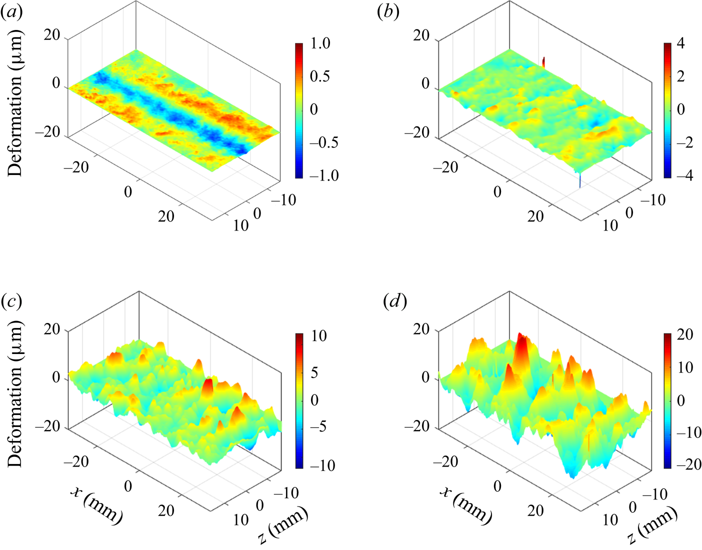
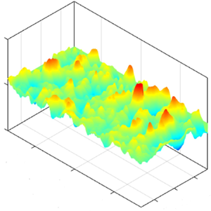
A sample raw fringe pattern is shown in figure 6(a), and the enhanced image, using the correlation-based fringe enhancement method (Zhang et al. Reference Zhang, Miorini and Katz2015, Reference Zhang, Wang, Blake and Katz2017) is presented in figure 6(b). The latter still has a few noisy spots with fringe discontinuity, preventing the use of simple phase unwrapping to determine the phase distribution. For these regions, the phase unwrapping is performed using a branch-cut method, i.e. the noisy spots are circumvented (Ghiglia, Mastin & Romero Reference Ghiglia, Mastin and Romero1987; Goldstein, Zebker & Werner Reference Goldstein, Zebker and Werner1988), as described in Zhang et al. (Reference Zhang, Wang, Blake and Katz2017). Once the phase distribution is determined over the entire image, the deformation map is calculated by spatial differentiation of adjacent iso-phase lines. Samples of instantaneous plots of (spatially detrended) deformation for U 0 ranging between 1.2 and 5.9 m s−1, corresponding to  $E/\rho U_0^2$ ranging from 59 to 2.4 are provided in figure 7. Three movies containing the time series of deformation at three different velocities are provided in the supplementary materials (see supplementary movies 1–3 available at https://doi.org/10.1017/jfm.2020.446). Several trends are evident. First, in agreement with the results of Rosti & Brandt (Reference Rosti and Brandt2017), at low speed, the typical surface pattern is aligned in the streamwise direction (see supplementary movie 1 and figure 7a), but with increasing velocity, the waves become preferentially aligned in the spanwise direction (see supplementary movies 2 and 3 and figure 7b–d). The likely origin of these streamwise-aligned and spanwise-aligned structures is discussed later. Second, the amplitude of deformations increases rapidly with decreasing
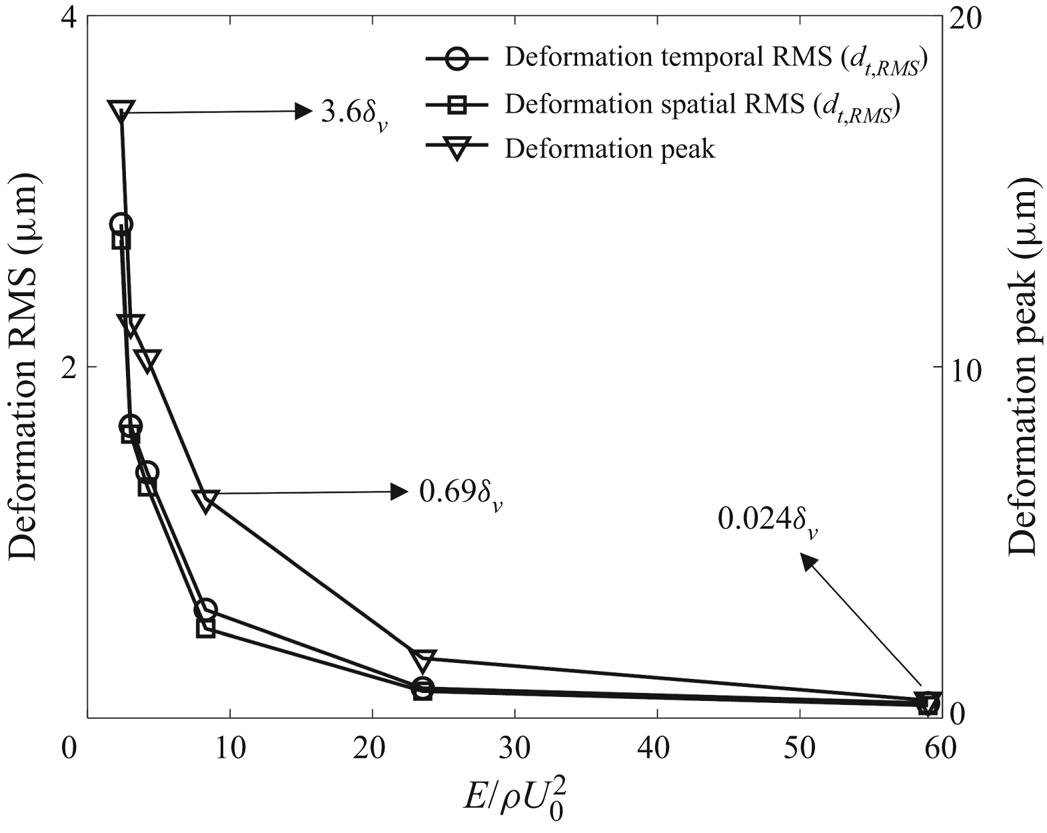
 $E/\rho U_0^2$. A corresponding plot quantifying this observation is presented in figure 8. It shows both the temporal root mean square deformation (dt ,RMS) at each point and then averaged over the entire field of view, the spatial root mean square of deformation (ds ,RMS) averaged over time, as well as the time average of the positive peak deformation (amplitude) in each realization. The values of dt ,RMS and ds ,RMS are also provided in table 1. The average peak increases from a submicron value at
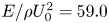 $E/\rho U_0^2 = 59.0$ to 18 μm at
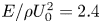 $E/\rho U_0^2 = 2.4$. As will be shown in the next section, the corresponding wall units decrease from 21 to 5 μm. Hence, while one-way coupling between deformation and flow might be expected for
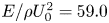 $E/\rho U_0^2 = 59.0$, the two-way coupling is likely to occur for
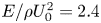 $E/\rho U_0^2 = 2.4$. However, as will be shown later, low levels of two-way coupling occur also at the lowest velocity.
Samples of compliant surface shape for U 0 and  $E/\rho U_0^2$ of: (a) 1.2 m s−1, 59.0; (b) 1.9 m s−1, 23.5; (c) 4.5 m s−1, 4.2 and (d) 5.9 m s−1, 2.4. While the axis scales are constant, the colour scales vary.

Variations of deformation peak as well as spatial and temporal r.m.s. values with  $E/\rho U_0^2$. Indicated values express the amplitude in terms of wall units.

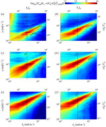
Third, unlike the rapid increase in magnitude, the length and width of deformation peaks do not change with velocity (decreasing  $E/\rho U_0^2$). These trends are demonstrated by examining the wavenumber–frequency spectra of the deformation. Figure 9 presents a series of streamwise wavenumber–frequency spectra, Edd(kx,ω), where the amplitude is normalized by [l 0dt ,RMS]2/U 0, kx is the streamwise wavenumber and ω is the frequency in rad s−1. The scales on the right and top sides of each plot provide the corresponding dimensionless frequency (ωl 0/U 0), and wavenumber (kxl 0). At this point, we opt to use l 0 as the length scale instead of, e.g. the boundary layer thickness as a basis of comparison with the Chase (Reference Chase1991) model (figure 1). The vertical lines mark the wavenumber corresponding to 3l 0, the range where the model predicts a peak response (figure 1). After subtracting the mean value and detrending the data along each streamwise line (similar to Zhang et al. Reference Zhang, Wang, Blake and Katz2017), these spectra are calculated in the streamwise direction and time for each spanwise location using fast Fourier transform (FFT) and then averaged over all spanwise planes. Each plot clearly shows an advected band with a phase speed of approximately 0.66U 0, as illustrated by the dashed lines in all the plots. This speed is slightly lower than the slow mode reported by Kim & Choi (Reference Kim and Choi2014) and in our previous experiment for a harder material (Zhang et al. Reference Zhang, Wang, Blake and Katz2017), namely 0.72U 0. Also, unlike our previous experiments, the present spectra do not show deformations travelling at the free-stream velocity. Furthermore, in all cases, the spectral peak of the advected band centres around a wavenumber corresponding to 3l 0, in clear agreement with the preferred wavelength predicted by the Chase (Reference Chase1991) model (figure 1). In spite of the increase in amplitude and changes to advection speed, the characteristic wavelength of advected deformations depends only on the thickness of the compliant layer. In addition, at low speeds, the kx − ω spectra have a band with high frequency and a very low wavenumber, which will be discussed later.
Streamwise wavenumber–frequency spectra of deformation for U 0 and  $E/\rho U_0^2$ of: (a) 1.2 m s−1, 59.0; (b) 1.9 m s−1, 23.5; (c) 3.2 m s−1, 8.3; (d) 4.5 m s−1, 4.2; (e) 5.3 m s−1, 3.0; and (f) 5.9 m s−1, 2.4. Dashed lines indicate an advection velocity of 0.66U 0, and solid lines indicate the wavenumber corresponding to 3l 0. Energy levels are scaled using
 $\textrm{log}_{10}[{E_{dd}}({k_x},\omega){U_0}/(l_0^2d_{t,\textit{RMS}}^2)]$, and the axes are presented both in dimensional and dimensionless forms.

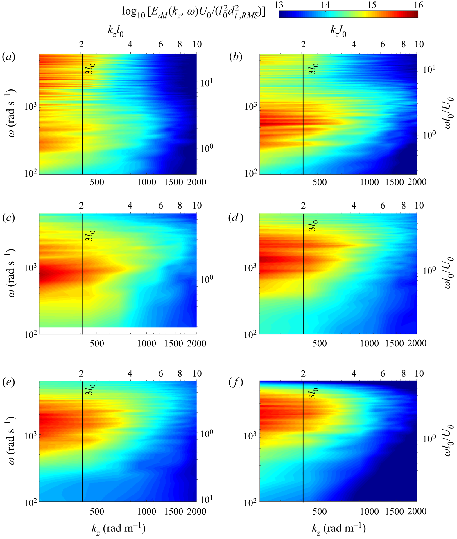
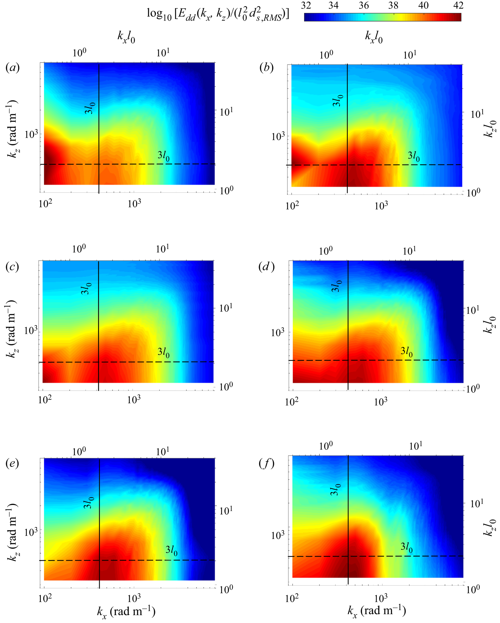
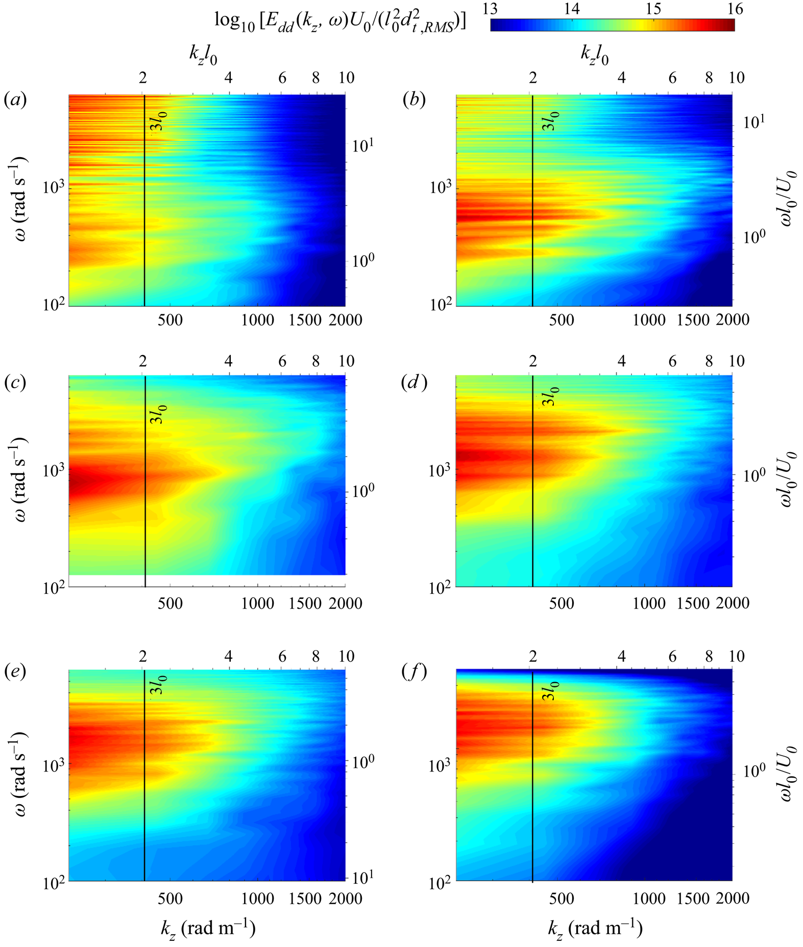
Corresponding plots of Edd(kz,ω) are presented in figure 10. Here, the FFTs are calculated in the spanwise directions and then averaged over all the streamwise planes. In this case, there is no evidence of an advected band, as expected. The primary spectral peaks have low wavenumbers that do not seem to vary significantly with velocity, remaining high up to a wavenumber corresponding to 3l 0. Again, consistent with the Chase (Reference Chase1991) model, it appears that the primary length scale affecting the deformation wavelength is the compliant layer thickness. In contrast, their frequency increases with velocity, and remains centred at around ωl 0/U 0 ~ 1.7. In addition, at low velocities, the kz − ω spectra have another low-wavenumber, high-frequency spectral band, that seems to coincide with the main band as the frequency of the latter shifts to higher values with increasing velocity. Finally, figure 11 shows the time-averaged two-dimensional spatial spectra, namely Edd(kx,kz). In this case, the results are normalized by the time-averaged spatial root-mean-square (r.m.s.) values (after subtracting the spatial mean and detrending), which are also given in table 1. Again, the spectra contain two peaks, which are distinct at low speeds, but the boundary between them becomes fuzzy with increasing velocity. The first peak is located at kz = 2π/3l 0 and very low kx. The second peak seems to be centred at low kz and kx slightly higher than 2π/3l 0, the predicted location of the peak in the Chase (Reference Chase1991) model. Otherwise, the (kx, kz) spectra do not seem to vary significantly with velocity. This trend implies that the wavelengths of the surface deformation in both directions are not associated with the flow scales. Hence, using the complaint wall thickness as a reference length scale is justified. The velocity affects the amplitude of these waves and their streamwise advection speed.
Spanwise wavenumber–frequency spectra of deformation for U 0 and  $E/\rho U_0^2$ of: (a) 1.2 m s−1, 59.0; (b) 1.9 m s−1, 23.5; (c) 3.2 m s−1, 8.3; (d) 4.5 m s−1, 4.2; (e) 5.3 m s−1, 3.0; and (f) 5.9 m s−1, 2.4.
Two-dimensional spectra of deformation for U 0 and  $E/\rho U_0^2$ of: (a) 1.2 m s−1, 59.0; (b) 1.9 m s−1, 23.5; (c) 3.2 m s−1, 8.3; (d) 4.5 m s−1, 4.2; (e) 5.3 m s−1, 3.0; and (f) 5.9 m s−1, 2.4. Both lines correspond to wavenumbers of 3l 0.

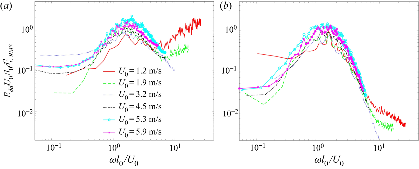
The next discussion compares the one-dimensional temporal spectra of deformation to predictions by two one-dimensional linear models, namely those of Chase (Reference Chase1991) and Benschop et al. (Reference Benschop, Greidanus, Delfos, Westerweel and Breugem2019). The experimental results for all the present speeds are presented in figure 12. Figure 12(a) shows the results for the entire range of measured wavenumbers, and figure 12(b) covers only the advected bands, i.e. the spectral range corresponding to advection speeds varying between 0.46 and 0.86U 0, as illustrated in figure 9(a). These spectra are calculated for every physical point in the sample area (after subtracting the mean value and detrending) and then spatially averaged. The frequency is normalized by U 0/l 0, and consequently, consistent with the trend evident in figure 9, all the main spectral peaks collapse to ωl 0/U 0 ~ 1.7. The energy is normalized by the corresponding r.m.s. values, hence the normalized peaks do not differ substantially in magnitude. Existence of the previously discussed high-frequency energy at low speeds is evident only in figure12(a), i.e. this range does not involve advected modes (as will be demonstrated later). In addition, all the spectra have a plateau at low frequency.
Temporal power spectral density of deformation for: (a) all wavenumbers and frequencies and (b) the advected bands  $(0.46{U_0} \lt \omega /k \lt 0.86{U_0})$.

The Chase (Reference Chase1991) model (referred to subsequently as the Chase model) solves the one-dimensional Helmholtz equation for the behaviour of a viscoelastic layer with a given thickness, shear modulus and loss tangent, which can be frequency dependent. The harmonic boundary conditions include flow-induced propagating pressure and shear waves with prescribed frequency and wavenumber, but the model also accounts for the acoustic impedance of the fluid medium. The results are given as closed-form equations for the spatially distributed material deformation. The Benschop et al. (Reference Benschop, Greidanus, Delfos, Westerweel and Breugem2019) model (referred to subsequently as the Benschop model) also solves the Helmholtz equation for given material properties, but the harmonic boundary conditions involve only pressure and shear stress waves propagating at a prescribed frequency and wavenumber. The results are also given as analytic expressions as a function of material properties, frequency and wavenumber. Both models predict that the impact of pressure is higher than that of the shear, hence the present discussion focuses on the effect of pressure. In applying these models, one has to consider the frequency-dependent amplitude of pressure excitation by the flow, as well as the frequency dependence of the material properties ((2.1) and figure 2). As noted before, the kx − ω spectrum presented in figure 1, which has been used for guiding the selection of the present material, assumes excitation at a uniform amplitude and fixed material properties. In this section, the analysis is repeated using both models, but this time it accounts for the characteristic pressure spectrum in a turbulent boundary layer as well as the measured frequency-dependent material properties. We have selected two pressure spectra for rigid wall boundary layers, the semi-theoretical one introduced by Goody (Reference Goody2004), and the one available from experimental wall pressure measurements by Tsuji et al. (Reference Tsuji, Fransson, Alfredsson and Johansson2007). Unfortunately, at the present time, we do not have wall pressure spectra for a flow modulated by the compliant wall, which would be more appropriate for this discussion. The experimental pressure spectra provided in Zhang et al. (Reference Zhang, Wang, Blake and Katz2017) for an-order-of-magnitude-harder complaint wall do not differ significantly from the rigid wall results as shown in Wang, Zhang & Katz (Reference Wang, Zhang and Katz2019). In Benschop et al. (Reference Benschop, Greidanus, Delfos, Westerweel and Breugem2019), the comparison is based on the experimental frequency spectrum. However, the dependence on wavenumber is modelled as advection at a frequency-dependent speed, which is assumed to decrease with increasing frequency. The present analysis is based on the measured kx − ω spectra for two types of excitations. The first covers only the advected bands between 0.46 and 0.86U 0 (figure 9a). The second analysis is based on the measured kx − ω spectra filtered at kx < 200.
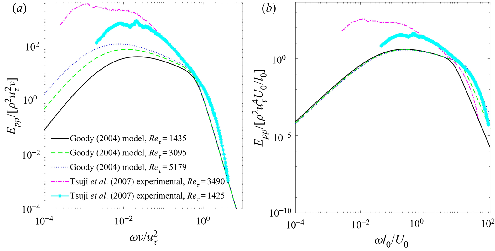
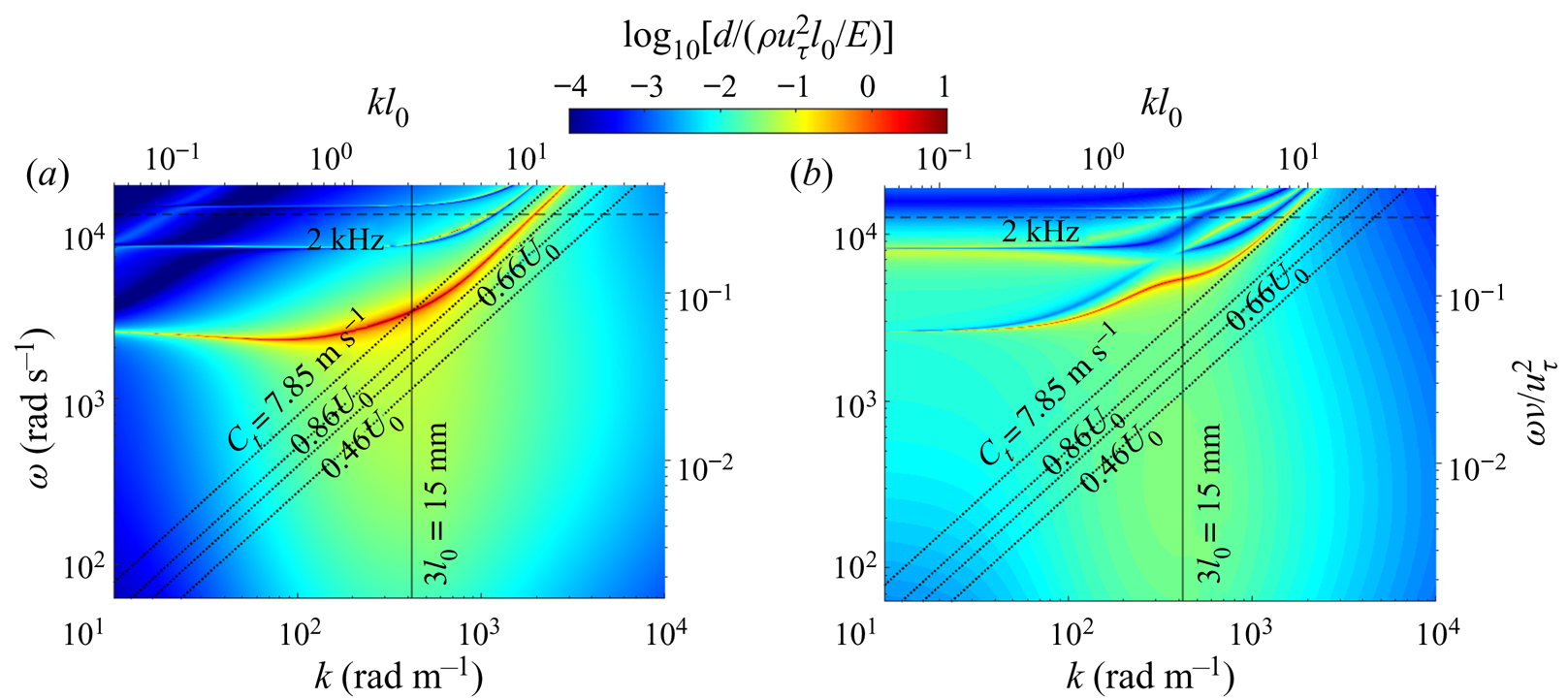
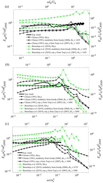
Figure 13 compares the two temporal pressure spectra used in the present analysis. In both cases, these spectra are Reynolds number dependent. The Goody (Reference Goody2004) spectra are given as an empirically determined analytic expression, and the Tsuji et al. (Reference Tsuji, Fransson, Alfredsson and Johansson2007) results are reproduced from the figures. They are both normalized using inner variables in figure 13(a). As is evident, with such scaling, differences exist mainly at low frequencies, but trends collapse at high frequency. The pressure spectra are also plotted in outer variables (figure 13b), showing a collapse at low frequency for Goody's pressure spectra. A comparison of wavenumber–frequency spectra obtained using the Chase and Benschop models is presented in figure 14(a,b), respectively. Both are based on the measured frequency-dependent material properties and the Goody's (Reference Goody2004) amplitude at the present highest Reynolds number. For the Chase model, the effect of accounting for the frequency dependence of excitation and properties can be observed by comparing figure 14(a) to figure 1. The primary difference occurs at low frequencies, where the reduction in excitation amplitude reduces the response in spite of the decrease in storage modulus and loss tangent (figure 2). In figure 14(a,b), both models show a response peak at a wavelength corresponding to three times the compliant coating thickness. However, the points of peak response differ, with the Benschop prediction having a higher frequency, and the Chase model showing a higher amplitude. However, the Benschop model has a broad area with the elevated response at low wavenumbers and high frequencies, peaking around  $\omega \nu /u_\tau ^2\sim 0.2$, although both have an elevated response in this range. Comparisons between the predictions of these models and the experimental results for the above-specified advection bands (figure 9a) at three different velocities are presented in figure 15(a–c). The experimental data also consist only of the advected band. Corresponding results for excitation at low wavenumber (k < 200 rad m−1) are presented in figure 16(a–c), with the experimental results also low-pass filtered at the same wavenumber. The (1-D) model predictions are provided for three pressure spectra, namely a pressure field with a uniform amplitude of
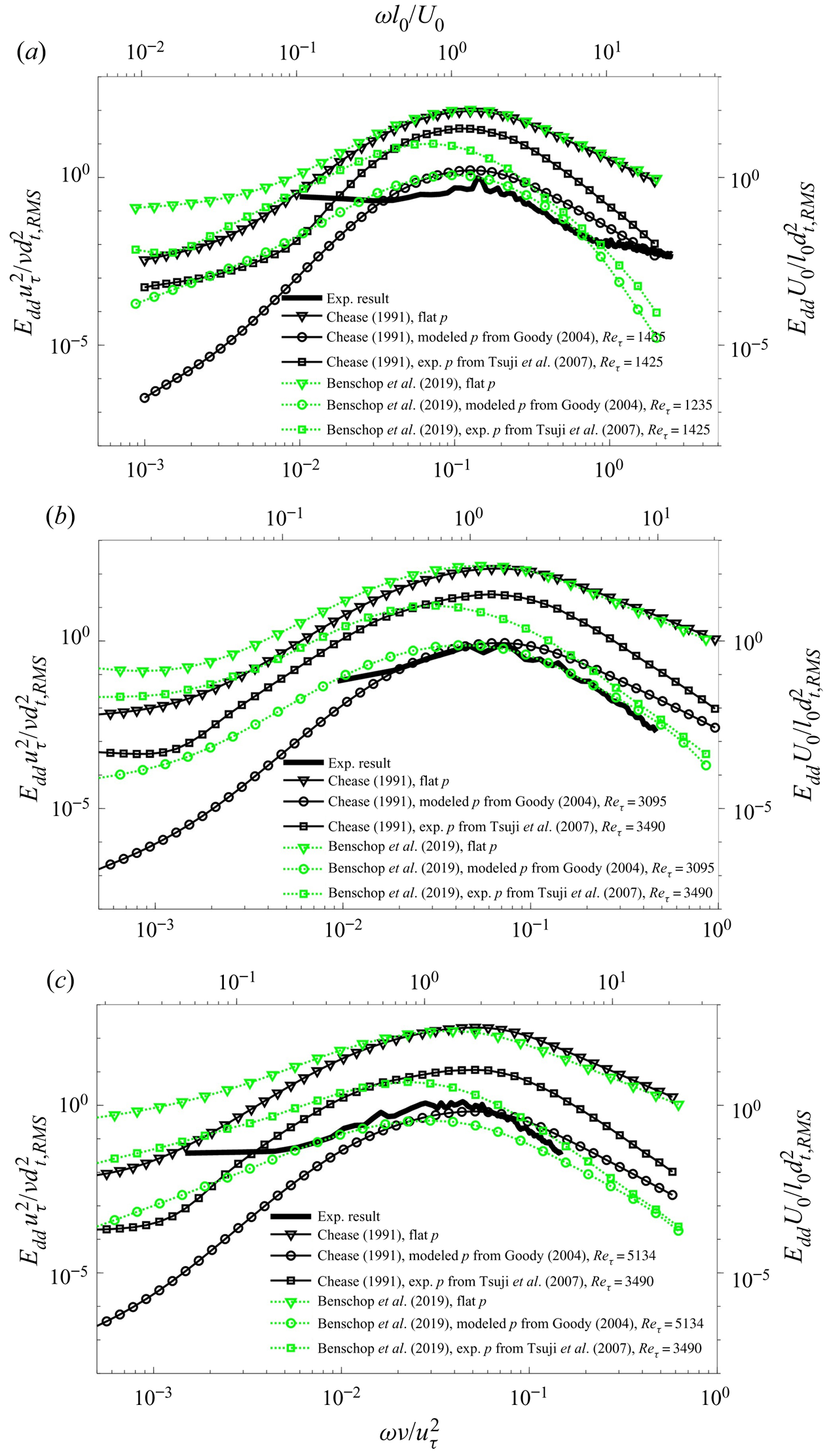
 $p^{\prime} = \rho u_\tau ^2$, as well as the Goody (Reference Goody2004) and Tsuji et al. (Reference Tsuji, Fransson, Alfredsson and Johansson2007) results (figure 13). The Goody spectra are calculated for the specific Reτ, while for the Tsuji spectra we use the Reτ = 1435 spectrum for the present lowest speed, and the results for Reτ = 3490 for higher speeds. In all cases, the analysis also accounts for the frequency dependence of the material properties. The frequency is normalized by inner variables at the bottom x-axis, and the energy, by the total experimental r.m.s. value (all frequencies and wavenumbers) and inner variables. Normalization of the frequency in outer variables are also provided in the top x-axis. Consequently, the comparison examines also the amplitude of the model predictions.
The pressure spectra from the Goody (Reference Goody2004) model and experimental measurement of Tsuji et al. (Reference Tsuji, Fransson, Alfredsson and Johansson2007) at different Reynolds numbers: (a) normalized by inner variables and (b) normalized by the outer variables.

The amplitude of deformation (normalized by  $\rho u_\tau ^2{l_0}/E$) in response to pressure perturbations modulated by the pressure spectra of Goody (Reference Goody2004), as predicted by: (a) the Chase (Reference Chase1991) model and (b) the Benschop et al. (Reference Benschop, Greidanus, Delfos, Westerweel and Breugem2019) models. Inclined dotted lines refer to advection bands at U 0 = 5.9 m s−1.
Comparison of the advected (0.46U 0 < ω/k < 0.86U 0) measured power spectra with the predictions by the Chase and Benschop models. The analysis is performed using the measured frequency-dependent material properties, and three different pressure excitations spectra, namely flat, Goody (Reference Goody2004) and Tsuji et al. (Reference Tsuji, Fransson, Alfredsson and Johansson2007). The corresponding U 0 and  $E/\rho U_0^2$ are: (a) 1.2 m s−1, 59.0; (b) 3.2 m s−1, 8.3 and (c) 5.9 m s−1, 2.4.

Comparison of the measured low-wavenumber power spectra (kx < 200 rad m−1) with predictions by the Chase and Benschop models. The corresponding U 0 and  $E/\rho U_0^2$ are: (a) 1.2 m s−1, 59.0; (b) 3.2 m s−1, 8.3 and (c) 5.9 m s−1, 2.4. Excitation amplitude and material properties are the same as those in figure 15.

For the advected bands, figure 15 demonstrates that around the spectral peak there is a good agreement between the measured events and the predictions of both models when the pressure is based on the Goody (Reference Goody2004) spectra. At low frequency, the Benschop results are higher and they tend to flatten more than the Chase predictions. Yet, neither model flattens to the same extent as the experimental data. At high frequency, the Chase predictions are higher with either Goody or Tsuji spectra, but the difference between the Chase predictions and the Benschop predictions is larger for the latter. These trends are consistent with those of the kx − ω spectra in figure 14. The magnitudes of the experimental high-frequency results appear to be more consistent with the Benschop model combined with Goody or Tsuji spectra. In all cases, predictions based on a flat pressure spectrum give significantly higher values than those based on experimental data.
As for the trends at low wavenumbers, figure 16 shows that the Benschop predictions are higher than those of the Chase model, consistent with the low kx range in figure 14. Also as expected, results for the flat pressure spectrum are higher than predictions based on the Goody or Tsuji pressure spectra. In general, trends of the experimental results differ from those of either model with maxima centred at different frequencies. Furthermore, the experimental results have a plateau or increase at high frequency, depending on velocity, in contrast to the model predictions. In terms of magnitude, for most of the spectra, the measured levels seem to fall in the same range as the Benschop model, higher than those calculated based on the Goody pressure spectrum and lower than that based on the Tsuji spectrum. We have also compared the experimental spectra to the model predictions for spatially low-pass filtered spanwise waves (not shown). Similar to figure 16, trends of the measured and modelled spectra do not agree. Furthermore, since this mode is not caused by the flow, a prediction by the flat pressure should be better. The predictions show a peak response at high frequency. Careful examination of this peak indicates that it is associated with deformation whose wavelength is 3l 0 travelling at the free shear-wave speed of the compliant material.
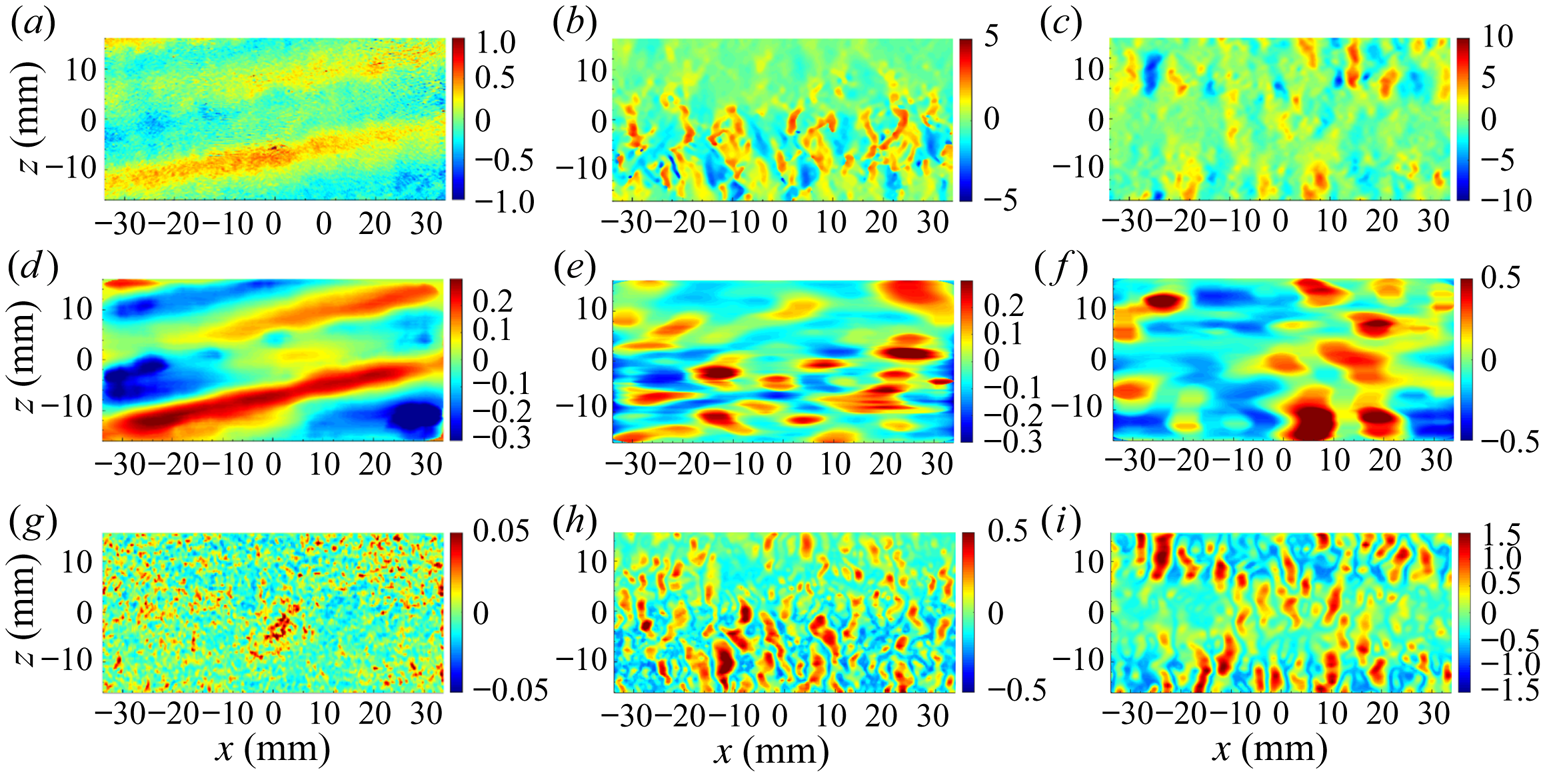
To elucidate the surface pattern associated with each of the above-mentioned spectral ranges, figure 17 provides a series of sample images. The unfiltered data presented in figure 17(a–c) are selected to show that spanwise-travelling waves persist even at high velocities, although they are not as obvious as those at low speed when the amplitude of advected modes decreases. Corresponding movies showing time series, hence not biased towards specific patterns, are provided as supplementary movies 1–3. Spatially low-pass filtered samples for kx < 200 are displayed in figure 17(d–f) for low and high velocities, respectively. The spanwise-travelling wave, with its crest aligned in the streamwise direction, is dominant at low speed. Its frequency is high (figure 9a), centred around 3000 rad s−1, and the dominant spanwise wavenumber is 400 rad m−1 (figure 11a), i.e. the corresponding advection speed is 7.5 m s−1, very close to the measured shear speed for the compliant wall. It appears that this phenomenon involves shear waves travelling laterally and presumably reflected from the side walls of the water tunnel. In the kx − kz spectra (figure 11a), the peak wavenumber of the spanwise shear wave corresponds to a wavelength of 3l 0, consistent with the model predictions, although the temporal spectra (figure 16a) do not agree. The time-resolved data (e.g. see supplementary movie 1) show that the transverse waves travel in both spanwise directions, i.e. they are not standing waves, and that they do not seem to be affected by local flow phenomena. At times, the wave is also inclined slightly (figure 17a,d), but the inclination angle varies without preferred direction. The specific energy source initiating these waves is unknown, and could involve large scale turbulence, pressure fluctuations or even tunnel vibrations. We presume that the preferred propagation in the spanwise direction is a result of reflections from the closer sidewalls of the water tunnel (88.5 mm from the centre), hence reflected disturbances are less likely to be attenuated. As illustrated in figure 4, while the edges of the compliant wall are free to move vertically, the horizontal motion is restricted to one direction. Owing to the high shear speed, figures 9 and 10 show that the corresponding spectral peaks reside in the upper left corner of the k–f spectra.
Deformation samples showing: (top row: a–c) the unfiltered signal, (middle row: d–f) low-pass filtered (kx < 200) signal and (bottom row: g–i): advected modes filtered at 0.46 < ω/k < 0.86. Flow conditions are: (left column: a, d and g) U 0 = 1.2 m s−1, and 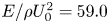 $E/\rho U_0^2 = 59.0$, (middle column: b, e and h) U 0 = 3.2 m s−1, and
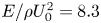 $E/\rho U_0^2 = 8.3$, and (right column: c, f and i) U 0 = 5.3 m s−1, and
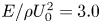 $E/\rho U_0^2 = 3.0$. Note the differences in scales.

When the velocity is increased (figure 17e,f), the surface structure becomes two-dimensional with both streamwise and spanwise waves, but clearly, the spanwise waves are still evident. Band-pass-filtered samples focusing on the (previously discussed) advected bands, corresponding to advection speeds ranging between 0.46 and 0.86U 0, are presented in figure 17(g–i). These waves seem to have a lattice structure, but with a crest preferentially oriented in the spanwise direction. This spanwise preference seems to increase with velocity, in agreement with the low Reynolds number DNS results of Rosti & Brandt (Reference Rosti and Brandt2017). The characteristic wavelength of these waves is also approximately 3l 0, consistent with both models and the measured advected band in the kx − ω spectra (figure9). In summary, the spanwise waves, which are dominant at low speeds, preferentially travel at the shear speed and have a preferred wavelength of 3l 0. These waves persist at high speed but appear to be overwhelmed by the advected mode, which also has a preferred wavelength of 3l 0, but their propagation speed is affected by the flow. As the shear speed and tunnel velocity get closer, the amplitude of these waves grows rapidly.
5. Velocity field above the compliant surface
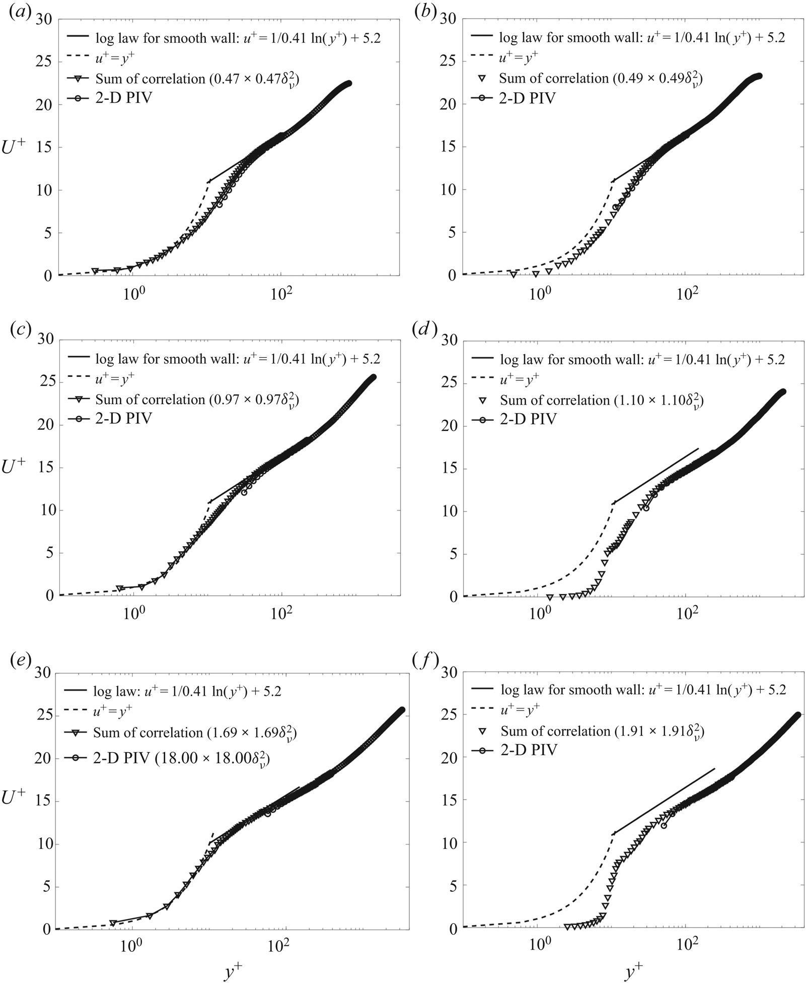
Figure 18 compares the mean velocity profiles above the rigid smooth (referred to as rigid in the following text) wall (figure 18a,c,e) to those above the compliant layer (figure 18b,d,f) at three velocities or  $E/\rho U_0^2$. Both the 2-D PIV and the sum-of-correlation results are presented. They nearly overlap except for lowest points where the standard results are too coarse. In all three cases, the rigid wall velocity profiles are consistent with those of a typical classical turbulent boundary layer with a viscous sublayer, buffer layer, log region that expands with increasing Reynolds number and parts of the outer layer. Measurements performed at a lower resolution, aimed at measuring the boundary layer thickness without resolving the inner region, have also been performed (not shown). The boundary layer parameters, including uτ and δν evaluated from a fit to the log layer and measured directly from the velocity profile in the viscous sublayer (y + < 5), as well as Reτ, are presented in table 1. The agreement between the two methods for calculating the wall shear stress suggests that the boundary layer over the rigid wall is fully developed. For the complaint wall profiles, uτ is calculated from a log layer fit. The above mentioned quantities are averaged along streamwise. The boundary layer scales listed in table 1 are spatially averaged along the streamwise direction. The spatial r.m.s. values of δν calculated from both the log fit and the viscous sublayer velocity gradient fall within 2 % of the averaged result, without a clear trend in the streamwise direction. Hence, the average values are used for the entire field of view (FOV).
Normalized mean velocity profiles calculated using sum-of-correlation PIV and standard 2-D PIV. Left column (a, c and e) rigid smooth wall data; and right column (b, d and f) compliant wall data. (a and b) U 0 = 1.2 m s−1, (c and d) U 0 = 3.2 m s−1 and (e and f) U 0 = 5.9 m s−1.

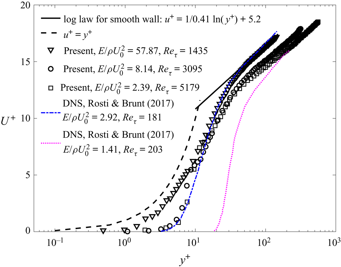
To highlight the effect of the compliant wall, figures 18(b,d,f), compares the velocity profiles to the standard viscous sublayer and log layer using the same constants as those of the rigid wall. As table 1 shows, except for the lowest velocity, where the values of uτ are very close to those of the rigid wall, for the higher speeds, the complaint wall increases the friction velocity by approximately 20 %. The velocity profiles begin to deviate from those of the typical boundary layer even at the lowest velocity (figure 18b), although the difference is quite small and the viscous sublayer is retained for the most part. Substantial deviations occur at U 0 = 3.2 m s−1 (figure 18d) and 5.9 m s−1 (figure 18f) when the amplitudes of the deformation (figure 8) are 0.69 and 3.6δν. Both show lower momentum in the log layer, and a sharp decrease in velocity at y + = 10 at U 0 = 3.2 m s−1, and y + = 13 at U 0 = 5.9 m s−1. Closer to the wall, the velocity gradients are small, which does not indicate low wall stress since the boundary is not stationary. Figure 19 compares the three velocity profiles to the DNS results of Rosti & Brandt (Reference Rosti and Brandt2017) for much lower Reynolds numbers, and except for one case, involve lower values of  $E/\rho U_0^2$. Yet, their profile for
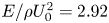 $E/\rho U_0^2 = 2.92$ and the present results for
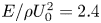 $E/\rho U_0^2 = 2.4$ (highest velocity) appear to have similar trends in the region of a sharp decrease in velocity in the inner part of the boundary layer. However, their zone of high-velocity gradients extends to a higher elevation. They also show that with decreasing
 $E/\rho U_0^2$, the region of sharp gradients shifts to a higher elevation, reducing the momentum in the log layer as well. The normalized r.m.s. values of deformation velocities by the inner variables
 $(\dot{d}_{t,\textit{RMS}}^+)$ are also presented in table 1, Rosti & Brandt (Reference Rosti and Brandt2017) observe that
 $\dot{d}_{\textit{RMS}}^ + = {{\rm \Delta} }{U^ + } {{\rm \Delta} }\kappa $, where
 ${{\rm \Delta} }{U^ + } $ is the momentum deficit in the log layer, and
 ${\rm \Delta} \kappa $ represents the change in the slope of the mean velocity profile in the log layer above the compliant wall. In their results for
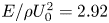 $E/\rho U_0^2 = 2.92$,
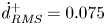 $\dot{d}_{\textit{RMS}}^ + = 0.075$, while in our measurement is 0.021 for a similar
 $E/\rho U_0^2$, i.e. they have the same order of magnitude.
The mean velocity profiles for the compliant wall turbulent boundary layer are compared with the DNS results of Rosti & Brandt (Reference Rosti and Brandt2017).

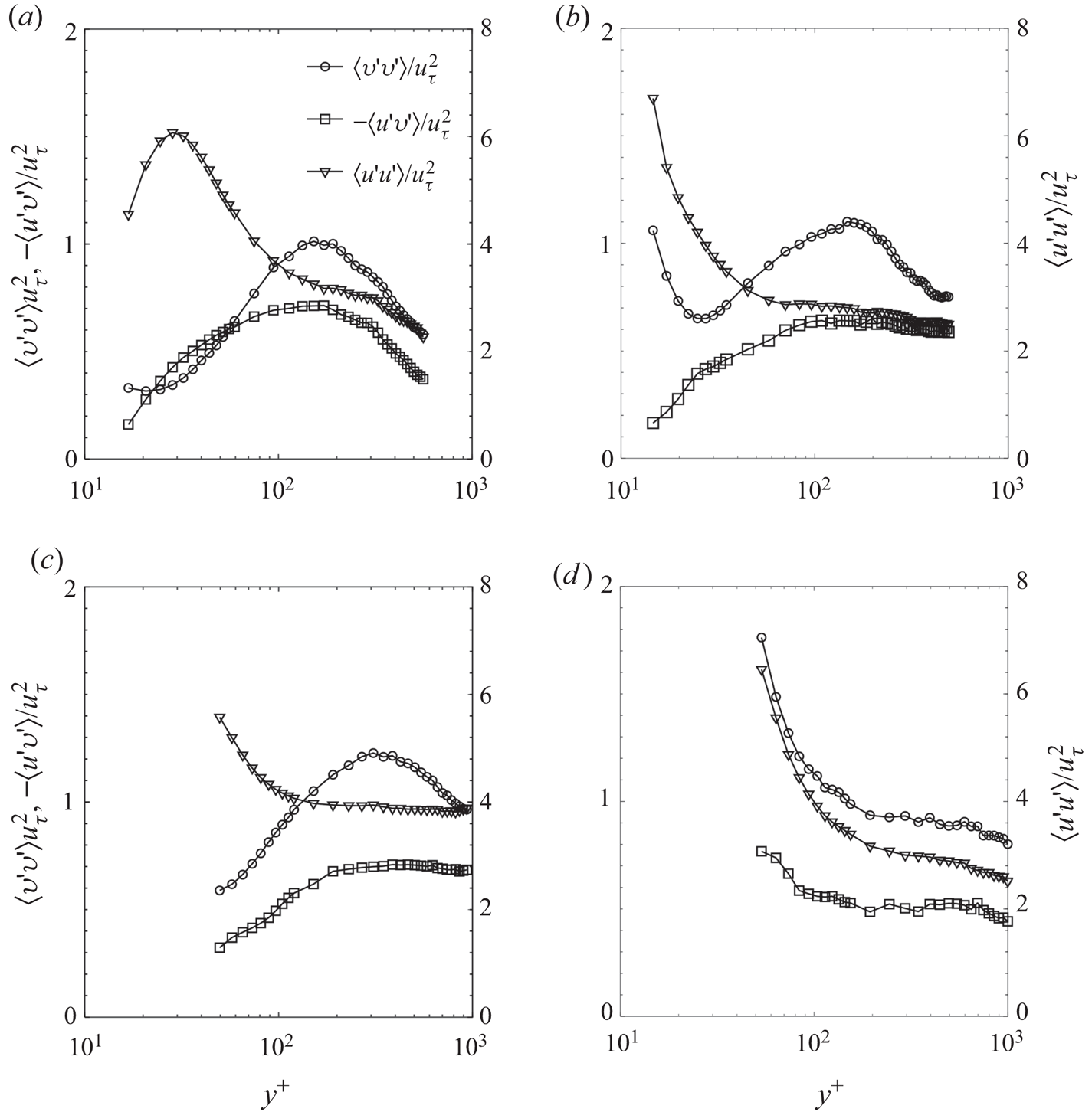
Profiles of Reynolds normal and shear stresses are compared to those of the rigid wall in figure 20. Owing to the limited spatial resolution of the present 2-D PIV measurements, the results are presented only for the lowest and intermediate free-stream velocities, and are limited to the elevation where the resolution-dependent uncertainty is below 0.5uτ (Wang et al. Reference Wang, Zhang and Katz2019). For the highest velocity, the interrogation window size is 20δν, making the results questionable for the relevant inner part of the boundary layer. This problem will be addressed in future studies by performing measurements at a higher resolution using, e.g. holographic microscopy (Sheng, Malkiel & Katz Reference Sheng, Malkiel and Katz2006; Gao & Katz Reference Gao and Katz2018). Results for the rigid wall are consistent with expectations. Even for the lowest velocity, above the compliant wall (figure 20b), there is a sharp increase in 〈v′v′〉 and 〈u′u′〉 near the wall, which does not involve an increase in −〈u′v′〉, i.e. the correlation among the components involved. This trend becomes stronger with increasing velocity (figure 20d), where the value of 〈v′v′〉 over the complaint wall (at the lowest data point) is three times higher than that of the rigid wall, and 〈u′u′〉 is 15 % higher. In this case, the shear stress also increases near the wall, but not at the same rate as the individual components. Rosti & Brandt (Reference Rosti and Brandt2017) also report an increase in turbulence level near the wall, especially 〈v′v′〉, as well as an increase in the shear stress at a slower pace compared to the individual components. These trends raise questions on the structure of the turbulence and associated length scales.
Reynolds stress profiles calculated using standard 2-D PIV for: left column (aandc) a rigid smooth wall; and right column (b and d) the compliant wall. (a and b) U 0 = 1.2 m s−1, and (c and d) U 0 = 3.2 m s−1. The scales for 〈v′v′〉 and −〈u′v′〉 are provided on the left axis, and those for 〈u′u′〉, on the right axis.

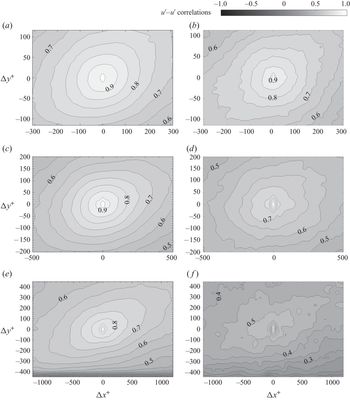
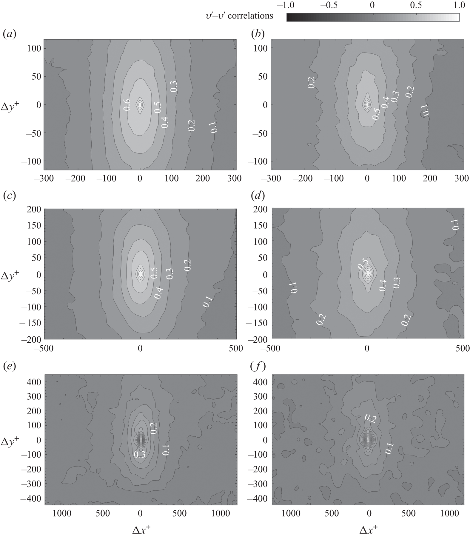
Glimpses of the extent of the changes to the log layer turbulence (y + = 600) are provided in figures 21 and 22 that compare u′–u′ and v′–v′ two-point correlations above the compliant coating to those of the rigid wall. As is evident, for both components, with increasing velocity or wall deformation amplitude relative to the wall unit, the correlation length scales diminish rapidly, suggesting that interactions with the wall ‘scramble’ the turbulence, making it much less coherent. However, the effects of wall deformation on the turbulence structure are evident even at the lowest velocity, i.e. when the deformation amplitude is much smaller than a wall unit (0.024δν, see figure 8). At the intermediate free-stream velocity (figures 21d and 22d), when the deformation amplitude is comparable to a wall unit (0.69δν), the wall motions are sufficient to cause a typical 20 % and 15 % reduction in u′–u′ and v′–v′ correlations at the same distance, respectively. When the deformation exceeds a wall unit (3.6δν), u′–u′ and v′–v′ correlations decrease by 55 % and 40 %, respectively. Clearly, even extremely small deformations are sufficient to cause two-way coupling with the mean flow and turbulence in the boundary layer. A reduction in the characteristic correlation length scales with decreasing  $E/\rho U_0^2$ has been observed also in the Rosti & Brandt (Reference Rosti and Brandt2017) simulations. Yet, they find an increase in the spanwise length scales that have not been measured in here, which they attribute to the preferred spanwise alignment of the deformation. As discussed before, in this study, the tendency towards a preferred spanwise alignment has only been observed with increasing velocity.
Two-point correlations of u′–u′ at y + = 600 for: (left column: a, c and e) smooth wall, and (right column: b, d and f) compliant wall at (a and b) U 0 = 1.2 m s−1, (c and d) U 0 = 3.2 m s−1 and (e and f) U 0 = 5.9 m s−1. Incremental increase between contour lines is 0.05.

Two-point correlations of v′–v′ at y + = 600 for: (left column: a, c and e) smooth wall, and (right column: b, d and f) compliant wall at (a and b) U 0 = 1.2 m s−1, (c and d) U 0 = 3.2 m s−1 and (e and f) U 0 = 5.9 m s−1. Incremental increase between contour lines is 0.05.

6. Discussion and conclusions
Expanding on a previous effort that has characterized the deformation of a relatively stiff compliant wall (Zhang et al. Reference Zhang, Wang, Blake and Katz2017), the present measurements focus on a compliant surface soft enough to deform to heights that modify the boundary layer structure, achieving two-way coupling. The surface properties are also selected, using a theoretical analysis introduced by Chase (Reference Chase1991), to fit within the wavenumber and frequency ranges of the data acquisition systems, enabling us to cover most of the important phenomena. The results show that the complaint wall deformation begins to impact the velocity profile when the amplitude of deformation is only a few per cent of the wall unit. When the amplitude is comparable to a wall unit or larger, the wall deformations cause a sharp decrease in momentum in the inner part of the boundary layer (less than 10 wall units). The turbulence level increases substantially, especially the wall-normal component, but the associated length scales decrease, i.e. the turbulence becomes more scrambled. The increase in turbulence level and decrease in u′–u′ and v′–v′ correlations with decreasing  $E/\rho U_0^2$ are consistent with trends described in Rosti & Brandt (Reference Rosti and Brandt2017). Furthermore, for the only case where their and our
 $E/\rho U_0^2$ values have the same magnitude, their velocity profile in the inner part of the boundary layer also shows a very similar sharp decrease at 4δν–10δν. However, their range of high-velocity gradients extends to a higher elevation, possibly because of the difference in Reynolds number. The corresponding present value of
 $\dot{d}_{t,\textit{RMS}}^ + $ is 0.021, whereas theirs is = 0.075, i.e. they are within the same order of magnitude.
The present values of 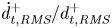 $\dot{d}_{t,\textit{RMS}}^ +{/}d_{t,\textit{RMS}}^ + $ decrease from 1 to 0.04 with increasing free-stream velocity (table 1). Hence, based on the discussions by Kim & Choi (Reference Kim and Choi2014), Xia, Huang & Xu (Reference Xia, Huang and Xu2017) and Benschop et al. (Reference Benschop, Greidanus, Delfos, Westerweel and Breugem2019), the wall velocity should affect the flow–wall interactions at low speeds, but not at high speeds, where the flow is expected to be impacted mostly by the displacement wave. However, while the magnitude of
 $\dot{d}_{t,\textit{RMS}}^ + $ is small over the entire present range of test conditions, varying between 0.004 and 0.021, the complaint surface motion still affects the flow, as suggested by the significant increase in 〈v′v′〉 above the wall with increasing
 $\dot{d}_{t,\textit{RMS}}^ + $. It should be noted also that based on the DNS results of Rosti & Brandt (Reference Rosti and Brandt2017), the wall streamwise velocity is smaller but of the same order of magnitude as the vertical component. Several reasons support our belief that the wall motion plays an important role in modifying the boundary layer structure. First, for rigid rough wall boundary layers, while an increase in roughness height of the order of the present
 $d_{t,\textit{RMS}}^ + $, i.e. from 0.004 to 0.54, is expected to increase the near-wall momentum deficit, this effect is typically small for roughness scales smaller than δν (Flack & Schultz Reference Flack and Schultz2014). Second, the few measurements performed in the inner part of rough wall boundary layers (e.g. Hong, Katz & Schultz Reference Hong, Katz and Schultz2011; Talapatra & Katz Reference Talapatra and Katz2012), and DNS data (e.g. Ikeda & Durbin Reference Ikeda and Durbin2007; Piomelli Reference Piomelli2019) have shown that the roughness does cause an increase in the wall-normal velocity fluctuations, but only very close to the wall, e.g. less than one roughness height in Talapatra & Katz (Reference Talapatra and Katz2012). In contrast, under the present conditions, figure 20 shows an increase in wall-normal fluctuations at elevations that are more than 100 times higher than
 $d_{t,\textit{RMS}}^ + $. Furthermore, this comparison does not even take into account the shallow ‘roughness slope’ of the compliant wall which, based on the values of
 ${d_{t,\textit{RMS}}}/3{l_0}$, is smaller than 0.01°. Hence, it is unlikely that the flow even separates above fixed surface bumps with the same geometry. Third, another possible wall–flow interaction might involve the pressure fluctuations induced by the oscillating boundary. The magnitudes of wall acceleration
 ${\ddot{d}_{t,\textit{RMS}}}$, also presented in table 1, are also significantly smaller than the corresponding values of
 $u_\tau ^3/\nu $ or
 $U_0^2/\delta$. Yet, in boundary layers, including those over a stiffer compliant wall
 $(E/\rho U_0^2\sim 220)$ reported in Zhang et al. (Reference Zhang, Wang, Blake and Katz2017), the pressure fluctuations have the highest correlations with the wall-normal velocity fluctuations. The same trend has been observed for rigid smooth wall boundary layers (Panton et al. Reference Panton, Goldamn, Lowery and Reischman1980; Joshi et al. Reference Joshi, Liu and Katz2014; Naka et al. Reference Naka, Stanislas, Foucaut, Coudert, Laval and Obi2015). Considering that the compliant wall causes a sharp increase in 〈v′v′〉 even at the lowest velocity (figure 20c), it is not unreasonable to postulate that the near-wall pressure fluctuations also increase. Finally, It should also be noted that trends of the present mean velocity profile are inconsistent with those of a turbulent boundary layer over a rough wall (e.g. Perry, Lim & Henbest Reference Perry, Lim and Henbest1987; Jimenez Reference Jimenez2003; Lee & Sung Reference Lee and Sung2007; Burattini et al. Reference Burattini, Leonardi, Orlandi and Antonia2008; Djenidi et al. Reference Djenidi, Antonia, Amielh and Anselmet2008; Hong et al. Reference Hong, Katz and Schultz2011, Reference Hong, Katz, Meneveau and Schultz2012), where the semi-log plotted velocity profile plateaus in the inner part of the boundary layer. In contrast, above the compliant wall, the velocity drops sharply and the turbulence is high well above the surface deformations. Furthermore, the profiles of Reynolds stresses differ substantially. Above rough boundaries, the turbulence level has a broad peak approximately four roughness heights away from the wall. It then decreases as the wall is approached, but rises again very close to the roughness elements, as mentioned above. These fundamental differences between the compliant wall and rough wall boundary layer suggest that one cannot view the deformed compliant surface as a rough boundary, and that the wall dynamics must be accounted for. These observations provide the rationale for performing detailed pressure fluctuation measurements near the compliant surface, which we plan to perform in subsequent studies.
Wavenumber–frequency and two-dimensional spectra show that the wall deformations consist primarily of two modes. The first is an advected mode that travels with the flow at 66 % of the free-stream velocity for all frequencies and wavenumbers. This velocity magnitude corresponds to the transition between the buffer layer to the log layer at y + = 60–80. In the prior experiments reported in Zhang et al. (Reference Zhang, Wang, Blake and Katz2017), the advection speed for a channel flow with a much stiffer wall is 72 % of the centreline velocity. The latter data also have another mode travelling at the free-stream velocity, which does not appear in the present results. We cannot give a substantiated explanation for the differences between these cases. They might be related to the differences between developing turbulent boundary layer and fully developed channel flow, or the fact that in the present study, the compliant wall deformations modify the boundary layer flow and Reynolds stress distributions. Future integrated 3-D flow and deformation measurements will attempt to answer this question. While the advected mode has a broad range of wavelengths, the spectral peak centres around 3l 0 for all cases. It also has a lattice-like structure, with preferential alignment on the spanwise direction. Frequency spectra for this mode nearly collapse if the frequency is scaled using the free-stream velocity and the compliant wall thickness.
With a primary advection speed being lower than the free-stream velocity (0.66U 0) and the previously observed pressure-deformation correlations showing a phase lag between the pressure and deformations for much stiffer complaint walls (Zhang et al. Reference Zhang, Wang, Blake and Katz2017), one wonders whether the present streamwise-advected phenomena are related to the TWF mentioned in the introduction. These theoretically derived instabilities are expected to grow in the streamwise direction, but not in time (Carpenter et al. Reference Carpenter, Davies and Lucey2000). Consequently, we have re-examined the data, and calculated the streamwise distribution of r.m.s. values of the un-detrended deformation, both for the entire data as well as for bandpass filtered data falling within the advected band (0.46–0.86U 0, see figure 9a). The results (not shown) indicate that while there several instantaneous realizations where the deformations appear to increase in amplitude in the streamwise direction, many others do not (see supplementary movies 2 and 3). Furthermore, the spatial distribution of r.m.s. values of deformation (not shown) do not show any evidence of an increase in the streamwise direction. Hence, while the magnitude of advection speed and a few of the instantaneous realizations are consistent with those TWF, one cannot say conclusively that they are related. The present results also do not show a slowly propagating high-amplitude waves resembling the static divergence waves. Their absence is consistent with the analysis performed by Carpenter & Garrad (Reference Carpenter and Garrad1986), which shows that the onset velocity for this phenomenon is approximately 1.8Ct, more than twice the present values.
The second mode travels predominantly in the spanwise direction and is concentrated in the low-wavenumber and high-frequency range. The kz − ω and kx − kz spectra show that this mode also has a characteristic wavelength of 3l 0, and travels at the shear speed of the compliant material irrespective of the free-stream velocity. When the tunnel speed is of the same order as the shear speed, the two modes coincide in the kz − ω spectra. At low speeds, the spanwise-travelling mode is dominant, but with increasing velocity, the advected modes take over. However, the spanwise mode persists at all velocities.
Both the present results and the simulations by Rosti & Brandt (Reference Rosti and Brandt2017) for much lower Reynolds numbers and softer materials show that the surface patterns are preferentially aligned in the streamwise direction at low velocity, and in the spanwise direction at high velocity. They attribute the low-velocity behaviour to the effects of low-speed streaks, which commonly occur in turbulent boundary layers. However, as noted above, the present measurements and analysis suggest that the streamwise-aligned pattern is associated with spanwise-travelling shear waves, which maintain the same wavelength with increasing Reynolds number, in contrast to trends of low-speed streaks, which have a typical wavelength of ~100δν (Smith & Metzler Reference Smith and Metzler1983; Brereton & Hwang Reference Brereton and Hwang1994). Furthermore, for the present conditions, the width of the low-speed streaks should be at least an order of magnitude smaller than the measured wavelength. In the Rosti & Brandt (Reference Rosti and Brandt2017) low Reynolds number simulations, 3l 0 ~ 270δν, i.e. the expected width of low-speed streaks are of the same order of magnitude as 3l 0.
Benschop et al. (Reference Benschop, Greidanus, Delfos, Westerweel and Breugem2019) fit their r.m.s. values of deformation for several speeds and material properties to the following empirical relation,  ${d_{t,\textit{RMS}}} = 0.031{l_0}{p^{\prime}_{\textit{rms}}}/G$. Here, G = E/[2(1 + νp)] is the shear modulus (νp is the Poisson ratio) and
 ${p^{\prime}_{\textit{rms}}}$ is the r.m.s. pressure fluctuation estimated by them using empirical data provided by Goody (Reference Goody2004), namely
 $p_{\textit{rms}}^ + = 0.0309 + 0.745{(\textrm{ln}({R_T}))^2}$ where RT = uτ/U 0Reτ. The present values of
 ${p^{\prime}_{\textit{rms}}}/G$, namely 2 × 10⁻³ – 5 × 10⁻³ are an order of magnitude smaller than those of Benschop et al. (Reference Benschop, Greidanus, Delfos, Westerweel and Breugem2019) since the compliant material is stiffer. Our measured r.m.s. level (figure 8) for the lowest velocity agrees with this empirical relation, but results deviate with increasing velocity, reaching values that are more than three times higher at U 0 = 5.9 m s−1. The Rosti & Brandt (Reference Rosti and Brandt2017) r.m.s. values normalized by inner variables are at the same level as our measurement for the matched
 $E/\rho U_0^2$.
Results of two previously published one-dimensional linear models of wall deformation by Chase (Reference Chase1991) and by Benschop et al. (Reference Benschop, Greidanus, Delfos, Westerweel and Breugem2019), which solve the same Helmholtz equations but with different boundary conditions, are used for elucidating the present trends. Both models predict a peak response at a wavelength of 3l 0 and at a frequency corresponding to the shear speed of the material. Differences predominantly occur at low wavenumbers and high frequencies. In comparing the frequency spectra to the model predictions, we account for the frequency dependence of both the material properties and the turbulent boundary layer pressure spectrum (Goody Reference Goody2004; Tsuji et al. Reference Tsuji, Fransson, Alfredsson and Johansson2007). For the advected mode, the models reproduce the spectral peak. Furthermore, the experimental amplitude most closely agrees with the Benschop model prediction using the Goody (Reference Goody2004) pressure spectrum, but the corresponding Chase (Reference Chase1991) results are not substantially different. If a uniform pressure spectrum is used instead, the predicted amplitude is substantially higher. In contrast, this approach does not reproduce the low-wavenumber fraction of the kx − ω spectrum, especially the high-frequency part. Yet, for excitation at a constant amplitude, both models predict a peak response at a wavelength of 3l 0 and frequency corresponding to the shear speed by the Chase model or slightly above it by the Benschop model. Hence, especially at low speed, when the excitation amplitude is low the surface should be expected to resonate at its peak response conditions, consistent with the experimental results. The remaining question involves the preferred alignment of such waves. Considering the rectangular shape of the compliant surface, a wave reflected from its boundaries travels a much shorter distance in the spanwise direction, suggesting that the spanwise-travelling wave would be stronger. The validity of these claims will be investigated in future studies.
Acknowledgements
This project has been funded by the Office of Naval Research under grant number N00014-16-1-2300. The programme officers are D. Nalchagian and G. Orris. The authors would also like to thank Y. Ronzhes who designed the water tunnel and J. T. Jose who assembled it.
Declaration of interests
The authors report no conflict of interest.
Supplementary movies
Supplementary movies are available at https://doi.org/10.1017/jfm.2020.446.