1 Introduction
The stable boundary layer (SBL) remains one of the least understood of all atmospheric boundary layers (ABL), due mainly to the complexity and diversity of phenomena it endures (Fernando & Weil Reference Fernando and Weil2010). The SBL is characterized by decreasing potential temperature with height, either continuously or in the form of steps (Nai-Ping, Neff & Kaimal Reference Nai-Ping, Neff and Kaimal1983). The stable stratification is formed due to (nocturnal) radiative cooling near the ground, which propagates upwards to tens of metres in height, determined by prevailing background conditions. The SBL can be classified into that on flat terrain and that on complex terrain, and is also identified in terms of very stable to weakly stable cases (Mahrt Reference Mahrt1998, Reference Mahrt2014). A large number of field studies have been conducted to understand processes that contribute to heat, momentum and scalar (moisture, pollutant) diffusion and transport in flat (Poulos et al. Reference Poulos, Blumen, Fritts, Lundquist, Sun, Burns, Nappo, Banta, Newsom and Cuxart2002) and complex (Doran, Fast & Horel Reference Doran, Fast and Horel2002; Fernando et al. Reference Fernando, Pardyjak, Di Sabatino, Chow, De Wekker, Hoch, Hacker, Pace, Pratt and Pu2015) terrain SBL. Reported laboratory studies are much fewer, because of the difficulty of obtaining suitable stratification in wind or water tunnels at high Reynolds numbers (Arya Reference Arya1972; Ohya Reference Ohya2001; Ohya, Nakamura & Uchida Reference Ohya, Nakamura and Uchida2008). Previous studies have identified a host of SBL phenomena, including propagating and trapped internal and inertial-gravity waves, low-level jets, instabilities, intrusions, fine-scale layering, flow meandering, eddies, and continuous and intermittent buoyancy-affected (stratified) turbulence. Additional flow types arise in complex terrain, for example, downslope (katabatic) and downvalley flows, critical (breaking) internal waves, lee waves, and sloshing of pooled cold air in confined valleys. The SBL phenomena span a swath of scales, from mesoscales (tens of kilometres) to turbulent kinetic energy (TKE) dissipation (millimetre) scales, and the latter, which have not been directly measured previously in the SBL, is the topic of this paper.
The regions of energy production in the SBL spectrum are usually assumed to spread over specific low-wavenumber ranges. A Kolmogorov inertial subrange is assumed to exist at still higher wavenumbers, followed by the TKE dissipation range. This assumption is particularly valid for the convective boundary layer (CBL) generated by ground heating or the neutral boundary layer driven by pressure gradients, where energy supplied at larger scales (
 ${\sim}100~\text{m}{-}1~\text{km}$
) is dissipated at Kolmogorov scales. With the general assumption that the TKE production occurs at low wavenumbers, the TKE dissipation rate
 $(\unicode[STIX]{x1D700})$
for most practical ABL situations is evaluated by assuming the validity of Kolmogorov theory, for example, by fitting Kolmogorov inertial subrange laws to measured energy spectra or structure functions (Kaimal & Finnigan Reference Kaimal and Finnigan1994; Davidson Reference Davidson2004); in practical applications,
 $\unicode[STIX]{x1D700}$
so evaluated is known as the eddy dissipation rate (EDR). In aviation, the EDR is educed using the aircraft response to turbulence (Sharman et al.
Reference Sharman, Cornman, Meymaris, Pearson and Farrar2014), whereas in ABL studies sonic anemometers are used to measure turbulent fluctuations and EDR with a spatial resolution of
 ${\sim}$
10 cm. While Kolmogorov turbulence is tenable for CBL and neutral ABL cases, SBLs have vertical length scales of the order of a few metres (Monti et al.
Reference Monti, Fernando, Princevac, Chan, Kowalewski and Pardyjak2002), and hence the applicability of classical inertial subrange and EDR concepts need to be viewed with caution because of the narrow inertial subrange. Mahrt (Reference Mahrt1998) argued that instrument resolution and post-processing may eliminate appreciable small-scale flux contributions to the total flux, calling for high-resolution measurements.
The above challenges were addressed in part during the field experimental phase of the Mountain Terrain Atmospheric Modeling and Observations (MATERHORN, 2011–2016) programme, which was designed to observe the ABL from mesoscale to energy-dissipating Kolmogorov scales
 $L_{K}=(\unicode[STIX]{x1D708}^{3}/\unicode[STIX]{x1D700})^{1/4}$
(
 $\unicode[STIX]{x1D708}$
is the kinematic viscosity) using an unprecedented suite of instrumentation (Fernando et al.
Reference Fernando, Pardyjak, Di Sabatino, Chow, De Wekker, Hoch, Hacker, Pace, Pratt and Pu2015). The finer scales were captured by hot-film probes, calibrated in situ using a co-located sonic anemometer, following Kit et al. (Reference Kit, Cherkassy, Saint and Fernando2010). The data encompassed a multitude of flow types that appear over different phases of the diurnal cycle, but careful winnowing of data allowed us to identify a period that fitted the rubric of stratified parallel shear flows, with all instruments functioning.
Such idealized conditions prevail only during limited time periods, but when present they can be of extraordinary importance in fundamental studies of stratified, sheared turbulence at very large Reynolds numbers
 $Re$
(based on the mean velocity
 $4~\text{m}~\text{s}^{-1}$
and the distance above ground
 ${\sim}$
6 m,
 $Re\sim 10^{6}{-}10^{7}$
). Observational SBL studies down to Kolmogorov scales have been rare, although dissipation estimations based on shear spectra of oceanic thermocline or TKE spectra of the SBL are more common and so are related stratified turbulence studies. A number of oceanic studies have reported measurements with Kolmogorov-scale resolution (Gargett, Osborn & Nasmyth Reference Gargett, Osborn and Nasmyth1984) but the Reynolds numbers achieved were limited and relevant background (synoptic) conditions have not been recorded.
Measurements presented in this paper show the presence of ‘bursts’ of significant velocity fluctuations at finer scales unresolved by sonics but captured via hot-film anemometry. The ensuing spectral bump can be frequent in the SBL, suggesting that conventional parametrizations for
 $\unicode[STIX]{x1D700}$
(i.e. via EDR estimates) may not be reliable. In a major outcome, we report on emerging fine-scale (
 ${\sim}$
0.1–0.4 m) turbulence at the high-wavenumber end of the ABL spectra through intermittent bursts, thus raising fundamental questions on existing frameworks of SBL modelling. The observational programme is outlined in § 2, and the characteristics of (serendipitously discovered) bursting phenomena are described in § 3. A discussion of possible bursting mechanisms, explanations of some observations and concluding remarks are given in § 4.
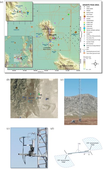
(a) Instrument placement during the autumn 2012 campaign of the MATERHORN programme. The main map is a bird’s-eye view around the Granite Peak; the upper left inset shows the details of the east slope (ES) site; and the bottom left inset depicts the expansive coverage of the Dugway Proving Ground. (b) Detailed zoomed locations of all five ES towers relative to Granite Peak east slope. (c) Combo probe comprising sonic and co-located hot-film multi-sensors. (d) A system of two combo probes covering
 $240^{\circ }$
measurement arcs. (e) ES-2 tower with Granite Peak in the background.

2 Field campaign, instrumentation challenges and methodology
Low space (
 ${\sim}$
10 cm) and time (
 ${\sim}$
16 Hz) resolutions of sonic anemometers limit their utility in fine-scale turbulence studies. The highest frequency that can be measured by a sonic of transducer separation
 $L$
in a flow of mean velocity
 $U$
is
 $f_{sa}=U/2\unicode[STIX]{x03C0}L$
(Kaimal & Finnigan Reference Kaimal and Finnigan1994). Hot-wire/film anemometry, on the other hand, has excellent spatio-temporal resolution suitable for resolving
 $\unicode[STIX]{x1D700}$
. The measurement requirements of hot-wire/film anemometry remain a challenge outside the laboratory, however, and lead to severe logistical challenges during field campaigns. First, the mean winds need to have a specific alignment with the hot-film/wire probe. Second, frequent and laborious calibrations are necessary for multi-sensor hot-film/wire probes, given their propensity for contamination and deterioration. Third, hot-wire probes are fragile and susceptible to breakage. Kit et al. (Reference Kit, Cherkassy, Saint and Fernando2010) averted these difficulties by conflating sonic and hot-film anemometers, so that their probe volumes are co-located, to reap the benefits of both probes. The mean wind vector was determined by averaging sonic data for a relatively short period (one minute). The coarse-resolution sonic measurements were employed to calibrate the hot films by deriving the output–input (velocity–voltage) transfer function for the hot film using a neural network (NN) model trained using low-pass-filtered hot-film and sonic data taken in situ (Kit et al.
Reference Kit, Cherkassy, Saint and Fernando2010; Vitkin et al.
Reference Vitkin, Liberzon, Grits and Kit2014; Kit & Liberzon Reference Kit and Liberzon2016). This probe system is called the ‘combo’ probe, which is shown in figure 1(c).
To follow the mean direction of variable atmospheric winds, a specialized mount was constructed to rigidly hold the sonic as well as the stepper motor that supported the hot-film holder. The stepper motor rotated the hot-film probes via the feedback signal derived using sonic-measured horizontal
 $(u,v)$
velocity components, which were interrogated at 1 min intervals and averaged over the last 5 s, as in Kit et al. (Reference Kit, Cherkassy, Saint and Fernando2010). This allowed sufficient time to filter out the smaller-scale variability of wind direction. Two combos were placed on a bar at the same height, and each swept through a
 $120^{\circ }$
measurement swath between the sonic ears, allowing
 $240^{\circ }$
total coverage by the two combos. This significantly improved the utility of multi-sensor hot-film probes by increasing the percentage of time the probes are aligned with the mean horizontal velocity. The horizontal velocity components measured by hot-film probe are presented in a coordinate system attached to the hot-film probe, with the
 $u$
-component aligned with the probe holder while the
 $v$
-component is orthogonal to that holder. A LabVIEW-based routine managed the data acquisition at a sampling frequency of 2 kHz while controlling the probe alignment. For simplicity, all data, including all four channels of sonic (three velocity components and temperature), were acquired at the same sampling frequency (2 kHz). This increased the required data storage space, but simplified the processing. The overall size of the multi-sensor hot-film probe used, which included two X-hot-film probes, is less than 7 mm, while the characteristic size of the probe volume of sonic is approximately 15 cm.
As mentioned, a double-combo system (figure 1 c,d) was deployed during the field campaigns of the MATERHORN project conducted at the Granite Mountain Atmospheric Sciences Testbed (GMAST) of the US Army Dugway Proving Ground (DPG), Utah (figure 1 a) – see Fernando & Pardyjak (Reference Fernando and Pardyjak2013) and Fernando et al. (Reference Fernando, Pardyjak, Di Sabatino, Chow, De Wekker, Hoch, Hacker, Pace, Pratt and Pu2015). The system (figure 1 d) was mounted at a height of 6 m on a 32 m high tower known as ES-2, which was a part of a densely instrumented flux tower array (ES-1–ES-5) designed to study stable stratified downslope (katabatic) flows at night on the east slope of the Granite Mountain (GM). ES-2 had seven levels of sonics: 0.4, 4, 10, 16, 20, 25 and 28 m. A full description of all instruments used and their locations can be found in Fernando et al. (Reference Fernando, Pardyjak, Di Sabatino, Chow, De Wekker, Hoch, Hacker, Pace, Pratt and Pu2015), and hence is not repeated here. This suite of instruments provided detailed information on the background mean flow. The focus of this paper is data taken during the MATERHORN autumn field campaign (25 September–31 October 2012) by instruments on the ES-2 tower, in particular, the combo-probe system.
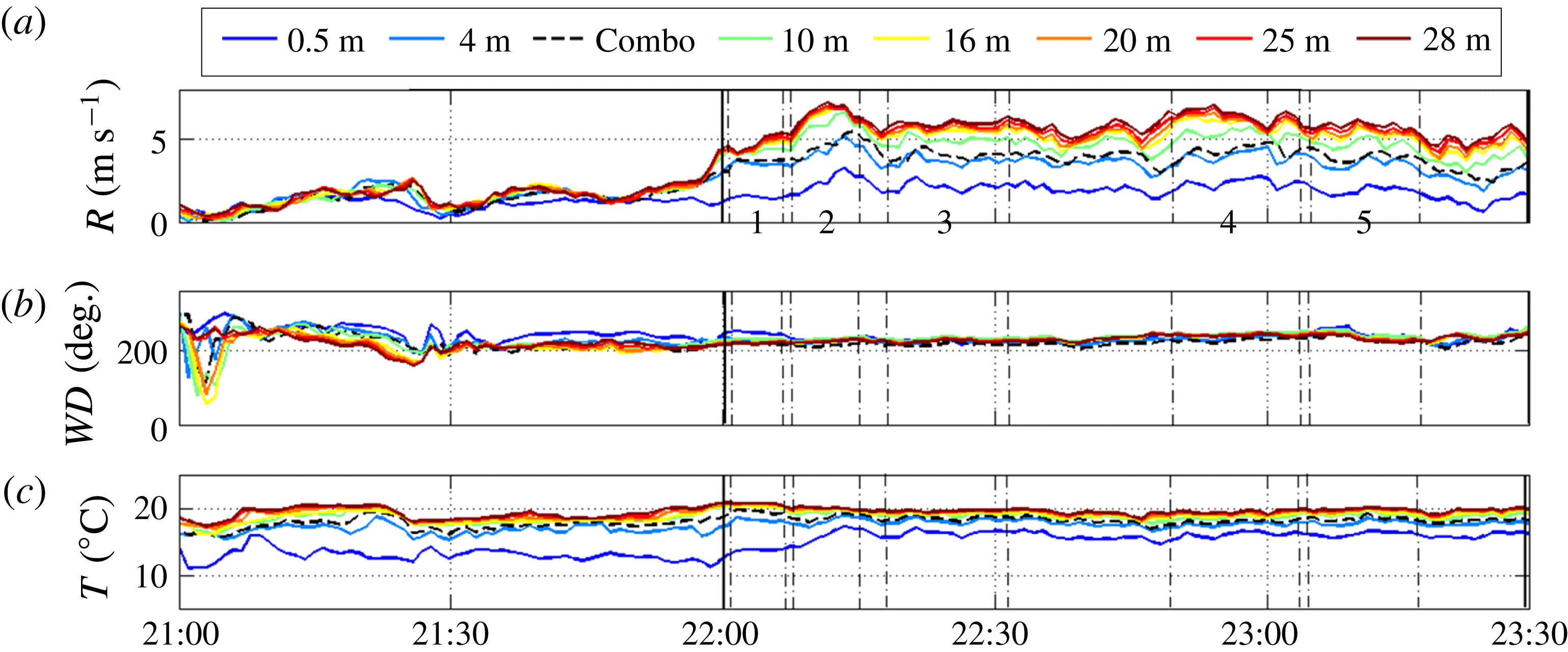
ES-2 background flow: (a) mean wind speed
 $R$
, (b) mean wind direction
 $WD$
, and (c) mean temperature
 $T$
(thermocouples) at different heights. The dashed line corresponds to the height of the combo probe. The period of analysis is marked by vertical solid lines and the subintervals (1–5) are indicated by vertical dashed lines. These are one minute averages. Time is MDT, and wind direction is measured from the north, clockwise (e.g. north to south indicates
 $0^{\circ }$
).

3 Results
3.1 General observations: background flow and turbulence
As in other natural complex terrain cases, the flow on the east slope was highly variable, but velocity profiles resembling a quasi-steady stratified parallel shear flow could be observed in the tower data for selected periods. Such periods captivate simplified analysis and comparison of data with theories developed for idealized flows. After careful processing of ES-2 sonic records and considering the data quality of hot films, the 90 min period following 22:00 MDT on the evening of 19 October 2012 was selected for stratified shear flow studies (MDT
 $=$
mountain daylight time (local time)). This selection was based on the fact that mean quantities were nominally quasi-steady during this period. As shown in figure 2(a), prior to this period, the wind speed rapidly increased from
 ${\sim}1~\text{m}~\text{s}^{-1}$
to
 ${\sim}4~\text{m}~\text{s}^{-1}$
at the height of the combo probe (6 m). The wind direction shifted from usual oscillations within the katabatic flow (Princevac & Fernando Reference Princevac and Fernando2008) before 22:00 MDT to a nearly constant
 ${\sim}230^{\circ }$
direction (figure 2
b) with stable temperature stratification (figure 2
c). This change was indicative of the change of forcing on the flow, as will be described later. Thereafter, the winds changed quite rapidly between 23:30 MDT and midnight (not shown).
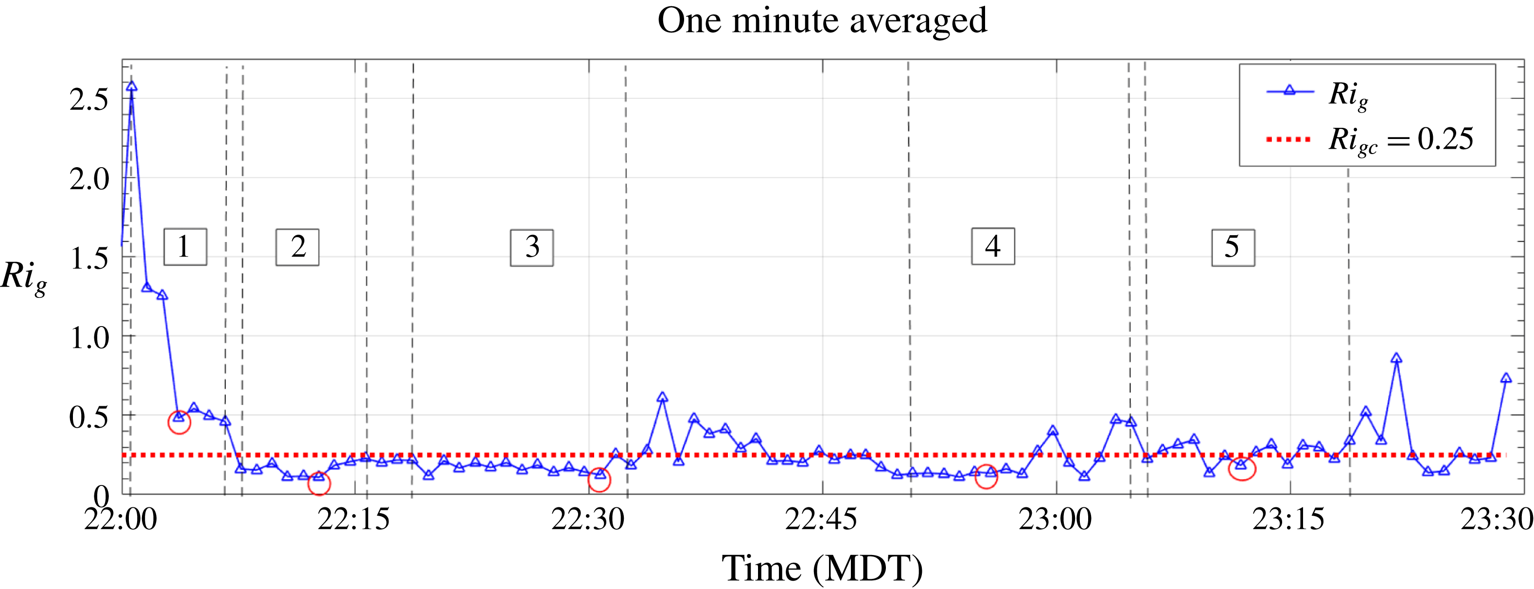
Plot of
 $Ri_{g}$
versus time at the combo height based on the one-minute-averaged sonic velocity and temperature gradients. See text for details. Red circles indicate regions for which the analysis is presented in the paper for bursting events. The periods of the subintervals (1–5) are marked by vertical dashed lines. Bursting was evident throughout the interval in varying degrees.

Although mean quantities were quasi-steady during the selected period 22:00-23:30 MDT, careful inspection of turbulence statistics showed considerable variability. Thus the analysis required identification of several homogeneous subintervals, which was based on the following criteria: (i) the interval should be relatively short to provide rather low/moderate variations of ambient conditions (
 ${<}$
15 min) but long enough for reliable statistics; (ii) the 1 min averaged mean and root-mean-square (r.m.s.) velocities vary only slightly across the subinterval; (iii) the variation of other turbulence statistics such as fluxes is moderate; and (iv) the skewness of the small-scale velocity gradients is negative, which is a requirement for enstrophy production in quasi-steady locally isotropic turbulence.
The five subintervals (
 $\text{SI}_{1}{-}\text{SI}_{5}$
) selected are shown in figure 2: first subinterval = 22:01–22:07 MDT, second = 22:08–22:15 MDT, third = 22:18–22:32 MDT, fourth = 22:50–23:04 MDT, and fifth = 23:05–23:18 MDT.
Before the analysis, it is important to further discuss the nature of the flow. In the MATERHORN autumn and spring (1–31 May 2013) experiments, the background flows in intense operational periods (IOPs) were categorized into synoptic classes, namely, quiescent (
 ${<}5~\text{m}~\text{s}^{-1}$
), moderate (
 $5{-}10~\text{m}~\text{s}^{-1}$
) and transitional (variable,
 ${>}10~\text{m}~\text{s}^{-1}$
possibly with frontal passages) – see Fernando et al. (Reference Fernando, Pardyjak, Di Sabatino, Chow, De Wekker, Hoch, Hacker, Pace, Pratt and Pu2015). Conventional katabatic flows driven by radiative cooling and having low-level jet features were observed only on quiescent days, and the studies on them were reported separately (Lehner et al.
Reference Lehner, Whiteman, Hoch, Jensen, Pardyjak, Leo, Di Sabatino and Fernando2015; Grachev et al.
Reference Grachev, Leo, Di Sabatino, Fernando, Pardyjak and Fairall2016). The data used for the present study were collected during flow transiting from a quiescent (IOP 8) to moderate (IOP 9) state, and it is likely that both pressure gradients and buoyancy (cooling) effects played a role in driving the flow.
In addition, the one-minute-averaged gradient Richardson number
 $Ri_{g}$
(a measure of SBL stability) based on temperatures at 5 and 7 m and polynomial-fitted velocity profiles at 4 and 10 m shows that it varies in the proximity of the critical value of
 $Ri_{gc}=0.25$
, indicating the importance of both the inertial and buoyancy effects (figure 3). Such flows are not expected to follow katabatic-flow characteristics such as jet-like velocity profiles.
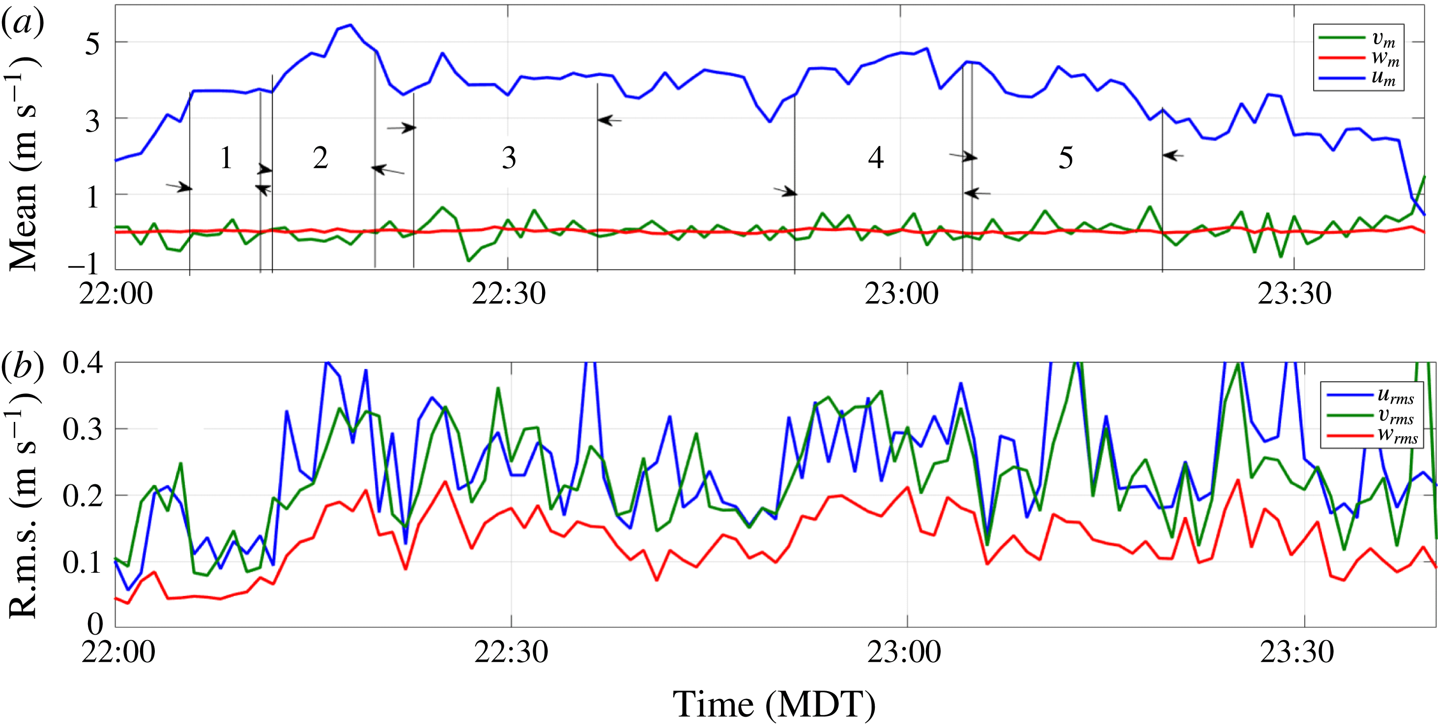
Figure 4 shows the mean and r.m.s. velocity components over the period of analysis (22:00–23:30 MDT).
(a) Mean and (b) r.m.s. horizontal (
 $u,v$
) and vertical (
 $w$
) velocities. The measurements were taken by sonic at the 6 m level above the ground.

Note that
 $\text{SI}_{1}$
(22:01–22:07 MDT) is characterized by TKE significantly smaller than that of other subintervals, suggesting a stage of turbulence development from the previous state of pure katabatic flow.
 $\text{SI}_{2}$
(22:08–22:16 MDT) and
 $\text{SI}_{3}$
(22:18–22:32 MDT) last for 8 and 14 min, respectively. The mean velocities changed significantly during these two time intervals and, as was observed during the processing, the turbulence varied intensely in both of them. Since they immediately follow the quasi-laminar first subinterval, these two subintervals can be construed as an interval of transition (the combined subinterval where transitioning-in regime occurs was dubbed
 $\text{SI}_{in}$
). In this regime, turbulent intensities and the TKE enhanced significantly (3–5 times). The end of
 $\text{SI}_{1}$
and the onset of
 $\text{SI}_{4}$
(22:50–23:04 MDT) are separated by 43 min, and the latter appear to represent a fully developed stage of turbulence, so as the initial part of
 $\text{SI}_{5}$
. The
 $\text{SI}_{4}$
particularly showed approximately constant velocity, stable turbulence statistics (e.g. skewness) and low variations of length scales, and hence was selected as a suitable period for studies of fully developed turbulence. Mostly we used a combined time interval that includes the entire
 $\text{SI}_{4}$
and the first 6 min of
 $\text{SI}_{5}$
to represent the developed stage of turbulence, and this subinterval was dubbed
 $\text{SI}_{devd}$
. During the remaining 7 min of
 $\text{SI}_{5}$
, the turbulence intensity decreased significantly and, thus, present again a transitioning-out period where developed turbulence is interrupted and non-stationary effects are emerging (e.g. strong bursting as occurred during
 $\text{SI}_{in}$
). This new subinterval was dubbed
 $\text{SI}_{out}$
.
In general, a one-minute interval is long enough to produce reliable mean values and short enough to suppose that the wind direction variation is relatively low. The in situ calibration procedure works properly when the mean wind velocity and direction are relatively fixed over the interval.
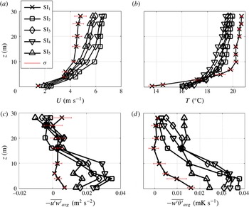
Figure 5 shows (1 min) averaged vertical profiles of mean velocity, temperature, Reynolds stresses and vertical heat fluxes calculated from sonics data. Note the similarities of profiles of subintervals 2–5, with Reynolds stresses and fluxes increasing towards the ground. Velocity profiles are similar to those of the moderately stratified boundary layers above.
For a horizontally homogeneous, stationary ABL, the Monin–Obukhov (MO) length scale,
 $L_{\ast }=-u_{\ast }^{3}/\unicode[STIX]{x1D705}q_{0}$
, where
 $q_{0}$
is the buoyancy flux,
 $\unicode[STIX]{x1D705}$
the von Karman constant and
 $u_{\ast }$
the friction velocity, is used to demarcate the height that separates the surface shear-dominated region
 $(z\ll L_{\ast })$
from the buoyancy-dominated region
 $(z\gg L_{\ast })$
aloft. In our work,
 $u_{\ast }$
and
 $q_{0}$
were assessed using the Reynolds stresses and virtual potential temperature flux computed from the two lower sonics (0.5 m and 4 m above the ground), and the results are presented in table 1. Note that, at the combo height
 $z=6~\text{m}$
, both buoyancy and shear can be considered as important, if the MO theory is locally applicable (as found by Grachev et al. (Reference Grachev, Leo, Di Sabatino, Fernando, Pardyjak and Fairall2016) for MATERHORN data). On the larger scales, however, there are noticeable horizontal temperature gradients, and hence advection in the flow direction should be accounted for in any computation of a property/energy balance (see Leo et al.
Reference Leo, Thompson, Di Sabatino and Fernando2016).
ES-2 (a) mean velocity
 $U$
, (b) mean temperature
 $T$
, (c) Reynolds stress
 $-\overline{u^{\prime }w^{\prime }}$
, and (d) heat flux
 $-\overline{w^{\prime }\unicode[STIX]{x1D703}^{\prime }}$
. One-minute averages are further averaged over subinterval lengths. The standard deviation
 $\unicode[STIX]{x1D70E}$
about the mean is shown as error bars for the first and second subintervals.

Monin–Obukhov length scale
 $L_{\ast }$
(m) computed using two lower sonics of ES-2 (0.5 m and 4 m above the ground).

In the first subinterval,
 $L_{\ast }<3~\text{m}$
, indicating that the combo-probe height, in a statistical sense, is largely disconnected from the surface shear, which is consistent with smaller Reynolds stresses (figure 5
c). The MO scale in quasi-steady
 $\text{SI}_{4}$
is
 $L_{\ast }\approx 12~\text{m}$
, where the effects of surface shear stresses are expected at the combo height. The non-stationary nature of the flow during
 $\text{SI}_{1}$
to
 $\text{SI}_{3}$
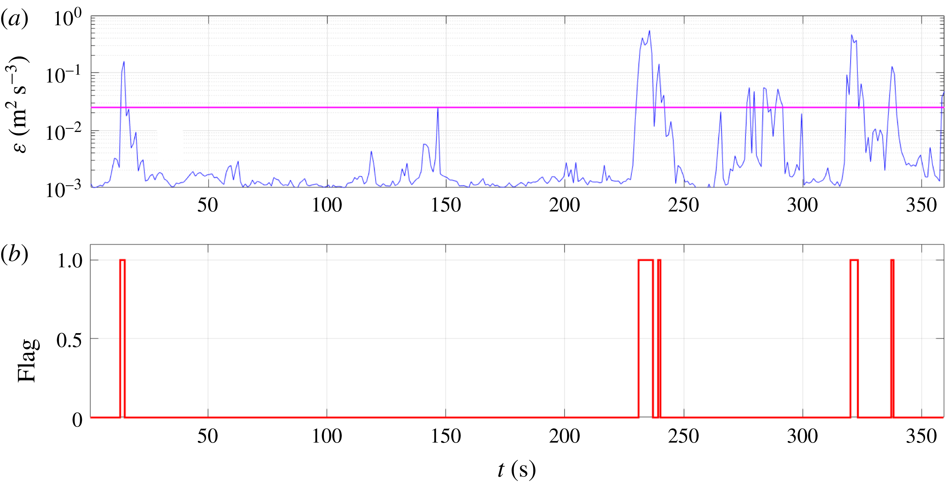
, however, limits the use of MO theory, and hence alternative parameters such as gradient Richardson number are better suited for interpreting the results (figure 4).
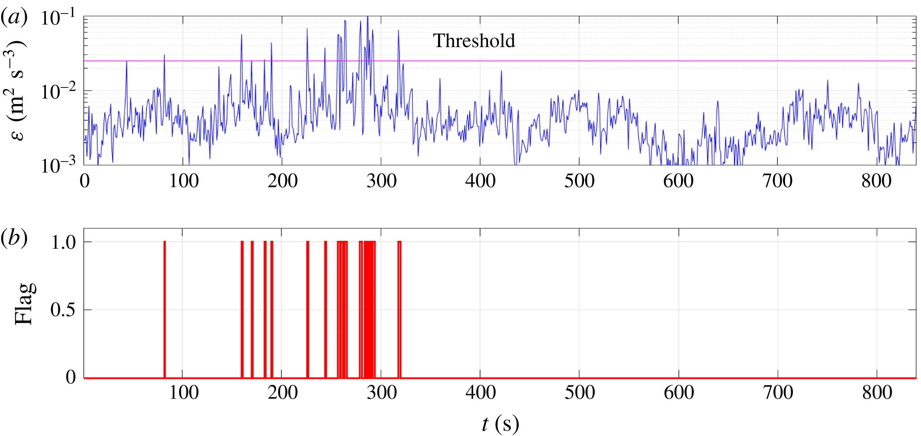
(a) Time series in
 $\text{SI}_{4}$
(22:50–23:04 MDT) of TKE dissipation rate
 $\unicode[STIX]{x1D700}_{u}$
versus time, with the horizontal line
 $\unicode[STIX]{x1D700}_{tr}=2.5\times 10^{-2}~\text{m}^{2}~\text{s}^{-3}$
. (b) Flag (
 $\unicode[STIX]{x1D700}>\unicode[STIX]{x1D700}_{tr}$
) separating times of elevated dissipation.

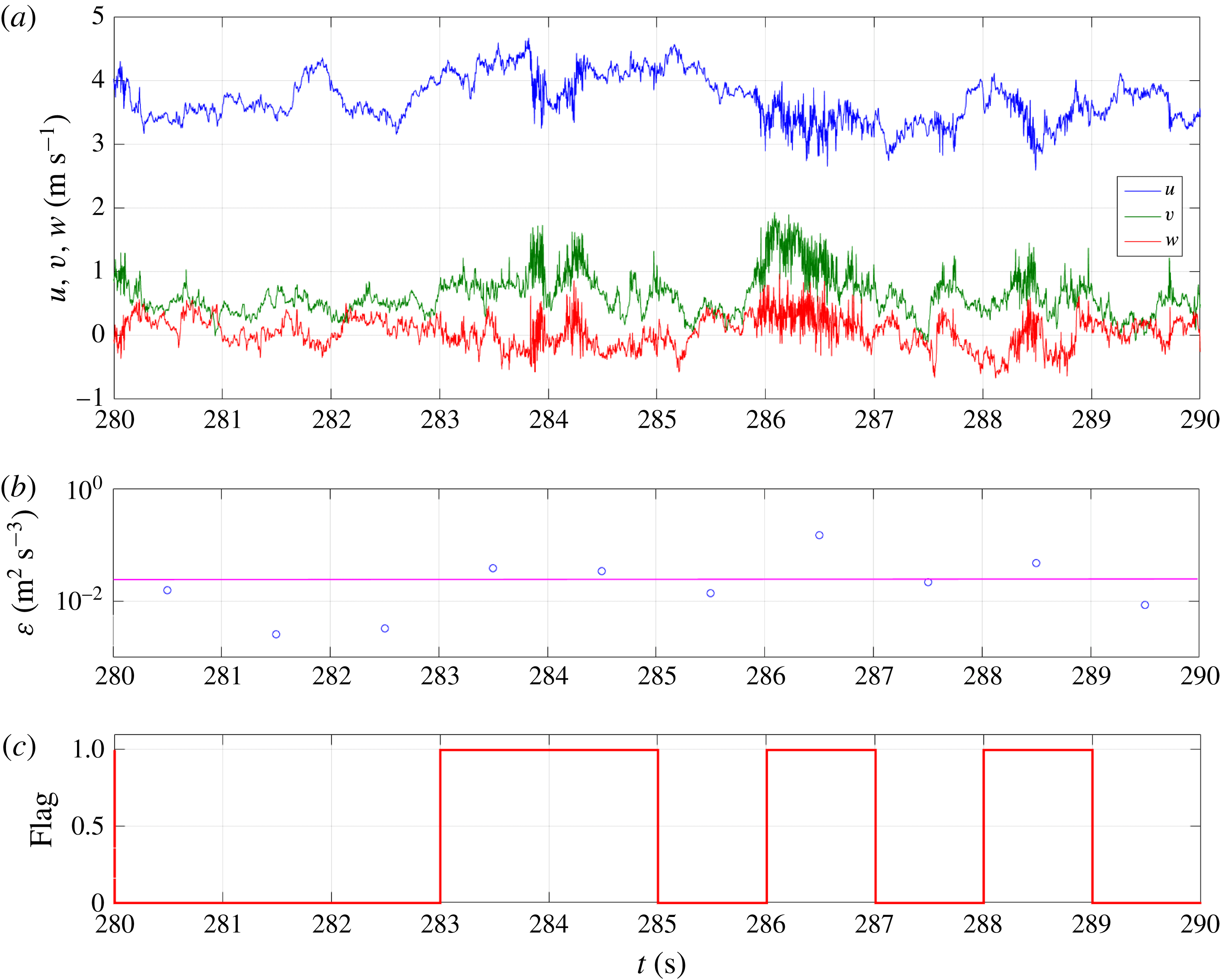
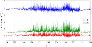
A 10 s time series segment of the fifth minute of
 $\text{SI}_{4}$
: (a) velocity components showing intermittingly present high-frequency bursts, (b) TKE dissipation rate
 $\unicode[STIX]{x1D700}$
computed using the
 $u$
velocity component (circles), and (c) flag separating 1 s time intervals which indicates bursting (
 $\unicode[STIX]{x1D700}>\unicode[STIX]{x1D700}_{tr}$
).

Another parameter employed in characterizing the SBL is the bulk Richardson number
 $Ri_{\unicode[STIX]{x1D6FF}}=\unicode[STIX]{x0394}b\unicode[STIX]{x1D6FF}/\unicode[STIX]{x0394}U^{2}$
defined in terms of a suitable SBL height
 $(\unicode[STIX]{x1D6FF})$
as well as the buoyancy (
 $\unicode[STIX]{x0394}b$
) and velocity
 $(\unicode[STIX]{x0394}U)$
jumps across it: neutral or weakly stable,
 $Ri_{\unicode[STIX]{x1D6FF}}<0.1$
; moderately stable,
 $0.1<Ri_{\unicode[STIX]{x1D6FF}}<0.5$
; and very stable,
 $Ri_{\unicode[STIX]{x1D6FF}}>0.5$
(Ohya Reference Ohya2001). While an accurate estimate of
 $\unicode[STIX]{x1D6FF}$
is difficult based on field measurements, the profiles measured with tethersondes with 30 min separation indicate
 $\unicode[STIX]{x1D6FF}\approx 15~\text{m}$
prior to the first interval and
 $\unicode[STIX]{x1D6FF}\approx 30~\text{m}$
during the rest of the period (not shown). Here
 $\unicode[STIX]{x1D6FF}$
is defined using a third-order polynomial fitted to tethersonde temperature profiles; the location where the velocity is 95 % of the maximum in the smoothed profile was taken as
 $\unicode[STIX]{x1D6FF}$
. When buoyancy/velocity jumps are calculated as that between the depth-averaged buoyancy/velocity below
 $\unicode[STIX]{x1D6FF}$
and the values just above it, the characteristic values become:
 $Ri_{\unicode[STIX]{x1D6FF}}\approx 0.6$
for the first subinterval (strongly stable, according to the definition of Ohya (Reference Ohya2001)) and
 $Ri_{\unicode[STIX]{x1D6FF}}\approx 0.18$
(moderately stable) for second to fifth subintervals. As expected, the first subinterval had a markedly different profile from the others, indicating a developing flow from a strongly stable to a moderately stable boundary layer.
The qualitative differences between the heat fluxes of
 $\text{SI}_{1}$
,
 $\text{SI}_{2}$
and
 $\text{SI}_{(3{-}5)}$
in figure 5(d) indicate the transitioning nature of the mean flow from a strongly stratified flow (based on Richardson number indicators in figure 3) to a moderately stable one. There are seeming hints of a low-level jet (though not as clear as in pure katabatic flows) in
 $\text{SI}_{2}{-}\text{SI}_{5}$
.
3.2 Analysis of turbulence in ‘developed’ flow
Figure 6 shows the hot-film measured velocity fluctuations and the TKE dissipation rate
 $\unicode[STIX]{x1D700}$
for
 $\text{SI}_{4}$
. Figure 6(a) contains the total TKE dissipation rate
 $\unicode[STIX]{x1D700}$
determined as
 $\unicode[STIX]{x1D700}_{u}=15\unicode[STIX]{x1D708}\overline{(\unicode[STIX]{x2202}u/\unicode[STIX]{x2202}x)^{2}}$
, with averaging conducted every second. The subscript
 $u$
indicates that computation is based on the longitudinal velocity component only. If local isotropy at small scales is assumed, the dissipation rate
 $\unicode[STIX]{x1D700}$
can be determined as
 $\unicode[STIX]{x1D700}_{v}=7.5\unicode[STIX]{x1D708}\overline{(\unicode[STIX]{x2202}v/\unicode[STIX]{x2202}x)^{2}},~\unicode[STIX]{x1D700}_{w}=7.5\unicode[STIX]{x1D708}\overline{(\unicode[STIX]{x2202}w/\unicode[STIX]{x2202}x)^{2}}$
using the two other velocity components. It follows from the following requirement for isotropy:
 $\overline{(\unicode[STIX]{x2202}v/\unicode[STIX]{x2202}x)^{2}}=\overline{(\unicode[STIX]{x2202}w/\unicode[STIX]{x2202}x)^{2}}=2\overline{(\unicode[STIX]{x2202}u/\unicode[STIX]{x2202}x)^{2}}$
. Here Taylor’s frozen turbulence hypothesis was used for computation of velocity derivatives in the flow direction. The averaging period in these calculations was 1 s, implying averaging over 2000 points at the sampling frequency
 $f_{s}=2~\text{kHz}$
to compute the block-averaged
 $\unicode[STIX]{x1D700}$
. Some relatively short bursting events, which are remarkably spasmodic, can be seen in figure 6. The background energy dissipation rate
 $\unicode[STIX]{x1D700}_{avg}$
, defined as the overall averaged dissipation rate for no-burst events only, is
 $\unicode[STIX]{x1D700}_{avg}=(4.5{-}5)\times 10^{-3}~\text{m}^{2}~\text{s}^{-3}$
, which is almost two orders of magnitude lower than the peak values of
 $1.5\times 10^{-1}~\text{m}^{2}~\text{s}^{-3}$
. To investigate this small-scale bursting phenomenon,
 $\text{SI}_{4}$
was partitioned into segments, where
 $\unicode[STIX]{x1D700}$
is above and below a threshold dissipation rate
 $\unicode[STIX]{x1D700}_{tr}$
. The selection of
 $\unicode[STIX]{x1D700}_{tr}$
is somewhat subjective, and was chosen to be approximately five times
 $\unicode[STIX]{x1D700}_{avg}$
. For
 $\text{SI}_{4}$
,
 $\unicode[STIX]{x1D700}_{tr}=2.5\times 10^{-2}~\text{m}^{2}~\text{s}^{-3}$
, and a flag of value 1 was assigned when the threshold is exceeded and was assigned 0 otherwise. The results are shown in figure 6(b), and the dissipation
 $\unicode[STIX]{x1D700}$
is elevated during the minutes 2–6, with noticeable peaks during the fifth minute. Therefore, the fifth minute of
 $\text{SI}_{4}$
was subjected to further analysis.
In particular, spasmodic dissipation variability prompted us to zoom in on a 10 s interval of the fifth minute, which led to the finding that intermittent, intense, high-frequency bursts are present in all velocity components (figure 7
a). The flagged periods of high
 $\unicode[STIX]{x1D700}$
are correlated with periods of bursts in velocity records, while
 $\unicode[STIX]{x1D700}$
reverts to the background dissipation when bursts are absent; compare figures 7(a) and 7(c).
It should be noted that canonical turbulence consists of intermittent periods with elevated dissipation levels, which is defined as the dissipation intermittency (see Sreenivasan & Antonia Reference Sreenivasan and Antonia1997). The bursts identified in our work, however, differ from the dissipation intermittency in that block-averaged (1 s)
 $\unicode[STIX]{x1D700}$
during the bursts are much stronger and often the dissipation is approximately two orders of magnitude larger than the background dissipation. The dissipation intermittency is present even in no-bursting time periods
 $(\unicode[STIX]{x1D700}<\unicode[STIX]{x1D700}_{tr})$
given that
 $\unicode[STIX]{x1D700}$
jumps to higher values intermittently, yet not high enough to cross
 $\unicode[STIX]{x1D700}_{tr}$
. In all, it is the order-of-magnitude larger
 $\unicode[STIX]{x1D700}$
compared to the background value that characterizes bursting. The intermittency of bursting reported here occurs at scales smaller than the scales of global intermittency and small-scale (inertial and larger) eddy front intermittency described by Mahrt (Reference Mahrt1989).
The separation of signal into burst/no-burst periods enabled investigations into spectral consequences of bursts. First, a data block of
 $T_{BR}=1~\text{s}$
was used for spectral computations. The spectral resolution that determines the lowest frequency
 $f_{L}$
and frequency difference
 $df=f_{i+1}-f_{i}=1/T_{BR}$
in the spectral computations is somewhat low (1 Hz). The highest tenable frequency is 1 kHz, which is the Nyquist frequency
 $f_{N}=0.5f_{s}=1~\text{kHz}$
, where
 $f_{s}$
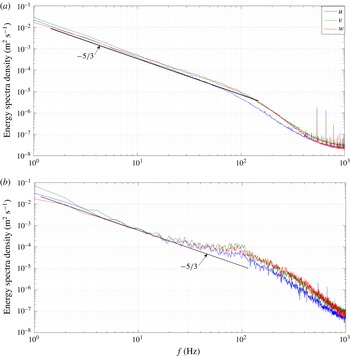
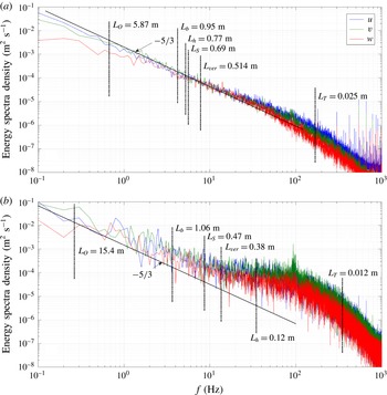
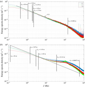
is the sampling frequency. The advantage of this approach is the improved accuracy of the averaged spectrum, since an ensemble average of plentiful 1 s spectral blocks is possible. In figure 8, the spectral density of velocity components of
 $\text{SI}_{4}$
is presented for periods without bursts (figure 8
a) and with bursts (figure 8
b). While time periods without bursts exhibit ideal shapes of Kolmogorov spectra over the accessible range of frequencies, those with bursts show a
 $-5/3$
slope only at lower frequencies.
Energy spectral density of velocity components computed within
 $\text{SI}_{4}$
: (a) no-burst records and (b) with-burst records. The total record of 840 s composed of 24 s of burst events and 816 s of no-burst events.

3.3 Spectral effects of bursts
The increased noise in the spectra with bursts shown in figure 8(b) is related to significantly smaller ensemble of records available for burst periods (24 versus 816), as evident from the burst/no-burst flag distribution (figure 6
b). To obtain better information on larger scales with potential stratification effects, improved spectral resolution is necessary, and therefore a longer time block was used for spectral computations, i.e.
 $T_{BR}=10~\text{s}$
instead of 1 s used before. Since many of the burst/no-burst data blocks span only a few seconds, here it was necessary to redefine a burst or no-burst block: if 1 s or less of bursting intervals were present within a 10 s block, then the entire block was considered burst-free, while if a burst spanning more than 1 s was present the block was considered a bursting event. In the following, the amalgamated interval comprising 14 minutes of
 $\text{SI}_{4}$
and the first 6 minutes of
 $\text{SI}_{5}$
containing no-burst events are considered together, referencing it as the developed flow
 $\text{SI}_{devd}$
. The rest of the
 $\text{SI}_{5}$
, where the developed flow is again terminated, was considered as a transitioning-out subinterval
 $\text{SI}_{out}$
where the flow started evolving rapidly. Both subintervals,
 $\text{SI}_{devd}$
and
 $\text{SI}_{out}$
, were analysed for burst/no-burst events and presented next.
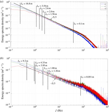
The higher-resolution (
 $T_{BR}=10~\text{s}$
) spectral results are shown in figure 9(a,b) for ensembles of data blocks with no bursts and bursts. Some relevant length scales are also indicated and are discussed later. The results are similar to those of the lower-resolution spectra of figure 8, with more noise in the spectra with bursts. Those with bursts deviate from the
 $-5/3$
slope, although the bump is smaller because many of the 10 s data blocks used in the fast Fourier transform comprised up to 8 s of no-burst data. At low frequencies, the spectrum of the vertical velocity is an order of magnitude smaller than that of longitudinal velocities, indicating suppression of the vertical velocity component by stratification therein, while preserving isotropy in the inertial range. (Note that, according to our selection, a 10 s burst interval contains at least 2 s of bursting events and a no-burst interval does not include more than 1 s of bursting. This selection is somewhat arbitrary. It would have been more appropriate, for example, to select blocks not containing bursts at all for the no-burst case, but it would decrease the ensemble size of no-bursting events in
 $\text{SI}_{devd}$
and
 $\text{SI}_{out}$
to an extremely low value.) In the following we will present only these high-resolution spectra based on 10 s contiguous blocks.
Same as for figure 8 for
 $\text{SI}_{4}$
but for
 $\text{SI}_{devd}$
with high resolution
 $\unicode[STIX]{x0394}f=0.1~\text{Hz}$
: (a) no-burst records and (b) burst records. Relevant length scales are indicated. The total record is 1200 s and was composed of 25 s of burst events and 1175 s of no-burst events.

Estimates based on r.m.s. velocity (
 $0.5~\text{m}~\text{s}^{-1}$
) and integral length scale (1.5 m) show that the eddy turnover time scale is
 ${\sim}3~\text{s}$
, and 10 s data blocks better capture the structure of the whole turbulence field (to the accuracy of Taylor’s frozen turbulence hypothesis) if it is stationary. Under these conditions, it is reasonable to expect a noticeable correlation between the energy-containing range and the dissipation range, with changes occurring at large scales manifesting at smaller scales after approximately an eddy turnover time according to classical Kolmogorov ideas (Fernando & Hunt Reference Fernando and Hunt1996). Indeed, this was clearly the case for no-burst periods in
 $\text{SI}_{devd}$
(not shown), and in the data records the changes of r.m.s. velocity preceded the response at dissipation scale by approximately an eddy turnover time scale (Pearson et al. (Reference Pearson, Yousef, Haugen, Brandenburg and Krogstad2004) also observed a similar result for their direct numerical simulations of turbulence). This, together with the spectral shapes, points to classical Kolmogorov turbulence during no-burst periods. Large-scale strong velocity fluctuations observed by Praskovsky & Oncley (Reference Praskovsky and Oncley1997) also appear to follow the above framework.
For burst periods, conversely, the correlation between large-scale fluctuations and dissipation estimated using the surrogate formulae presented above was very low, suggesting departure from the classical Kolmogorov turbulence. The bumps in the burst spectra suggest this departure may be due to modification of energy cascade at the high-frequency end of the inertial subrange. The observations of spasmodic dissipation events (bursts) and near-simultaneous strong increase of spectral densities at scales in the realm of the Taylor microscale
 $L_{T}$
, with spectral deviations starting from almost the shear scales
 $L_{s}$
(defined below), is incongruent with the classical energy cascade; see, for example, figures 6 and 7. There is a crucial need to explain the burst events and the scales of energy injection therein that lead to development of a significant bump in the energy spectra at higher frequencies.
To further understand the effects of stratification on turbulence, canonical characteristic length scales evaluated at the combo height are presented in figure 9, which include the Ozmidov length scale
 $L_{O}=(\unicode[STIX]{x1D700}/N^{3})^{1/2}$
, the buoyancy length scale
 $L_{b}=\unicode[STIX]{x1D70E}_{u}/N$
, and the vertical scale of stratified turbulence
 $L_{ver}=\unicode[STIX]{x1D70E}_{w}/N$
. Additional scales relevant to shear flows are
 $L_{s}=\unicode[STIX]{x1D70E}_{u}/(\unicode[STIX]{x2202}\bar{U}/\unicode[STIX]{x2202}z)$
, the Taylor microscale
 $L_{T}=(\unicode[STIX]{x1D70E}_{u}^{2}/\overline{(\unicode[STIX]{x2202}u/\unicode[STIX]{x2202}x)^{2}})^{1/2}$
and the horizontal scale of stratified turbulence
 $L_{h}=\unicode[STIX]{x1D70E}_{u}^{3}/\unicode[STIX]{x1D700}$
(see Riley & Lindborg Reference Riley and Lindborg2008). Here
 $N^{2}=g\unicode[STIX]{x1D6FC}\,\text{d}\unicode[STIX]{x1D703}/\text{d}z$
is the Brunt–Väisälä frequency,
 $\unicode[STIX]{x1D703}$
the potential temperature,
 $z$
the vertical coordinate,
 $\unicode[STIX]{x1D6FC}$
the coefficient of thermal expansion, (
 $\unicode[STIX]{x1D70E}_{u},\unicode[STIX]{x1D70E}_{w}$
) the r.m.s. horizontal and vertical velocities,
 $\unicode[STIX]{x1D708}$
the kinematic viscosity and
 $\bar{U}$
the mean velocity.
An important characteristic of turbulence is the skewness of the longitudinal velocity derivative
 $S=\overline{(\unicode[STIX]{x2202}u/\unicode[STIX]{x2202}x)^{3}}/(\overline{(\unicode[STIX]{x2202}u/\unicode[STIX]{x2202}x)^{2}})^{3/2}$
, which is related to enstrophy generation. For isotropic turbulence, simple relations between the skewness and enstrophy generation term can be derived (Champagne Reference Champagne1978). In the literature,
 $S$
has been computed directly using the above expression (Batchelor & Townsend Reference Batchelor and Townsend1947; Champagne Reference Champagne1978; Arora & Azad Reference Arora and Azad1980; Van Atta & Antonia Reference Van Atta and Antonia1980; Tsinober, Kit & Dracos Reference Tsinober, Kit and Dracos1992; Sreenivasan & Antonia Reference Sreenivasan and Antonia1997; Shen & Warhaft Reference Shen and Warhaft2000), using integral expressions in the spectral domain (Smith & Reynolds Reference Smith and Reynolds1991; Nelkin Reference Nelkin1994), multifractal-based approaches (Chevillard et al.
Reference Chevillard, Castaing, Levequ and Arneodo2006) or matched asymptotic expansion (Lundgren Reference Lundgren2008). Wind tunnel studies as well as theoretical approaches indicate
 $S\sim -0.4$
. We calculated
 $S$
directly for each second of
 $\text{SI}_{devd}$
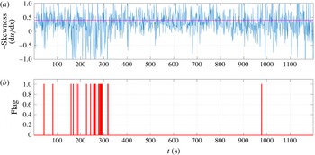
(figure 10), which oscillated around
 $-0.4$
for all segments without bursts. During minutes 3, 4 and 5, when bursting is significant or sometimes even dominating, the skewness strongly fluctuated with a mean value other than
 $-0.4$
, possibly indicating the emergence of new dynamics due to bursting rather than conventional enstrophy generation that would have been dominant otherwise.
Below, we present results for other subintervals, starting with
 $\text{SI}_{5}$
(23:05–23:18 MDT). As mentioned, bursting is absent during the first 6 minutes; much like a continuation of
 $\text{SI}_{4}$
(figure 6), it was considered a part of
 $\text{SI}_{devd}$
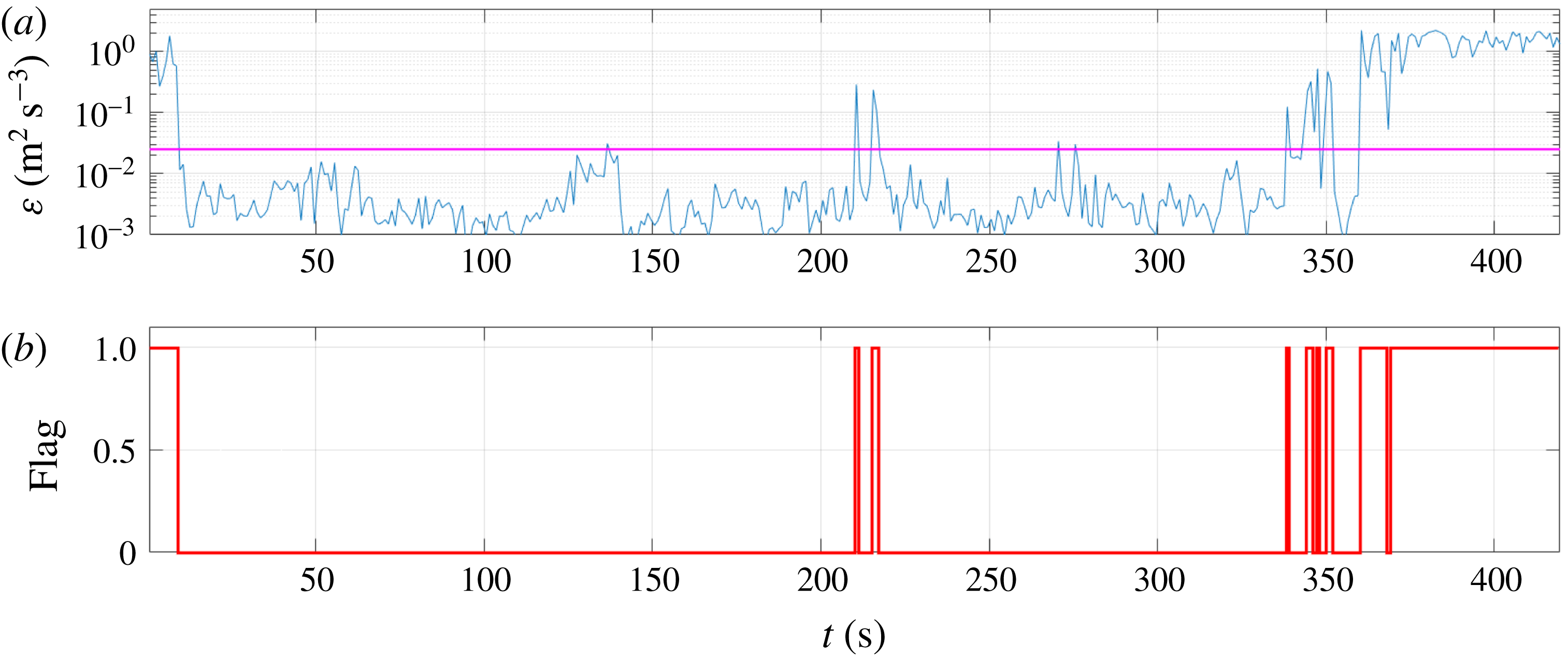
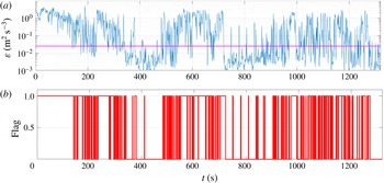
. Very strong bursts developed in the seventh minute of
 $\text{SI}_{out}$
(figure 11), characterized by a spiky dissipation rate, which is almost three orders of magnitude higher than the background value. During the last 2 minutes, the 12th and 13th, bursting was rampant and almost continuous during the entire 13th minute.
Times series of (a) negative skewness (
 $S$
) of the longitudinal velocity derivative for combined interval
 $\text{SI}_{devd}$
and (b) burst/no-burst flag. The horizontal line indicates
 $S=-0.4$
.

Time series of (a) kinetic energy dissipation rate for transitioning-out
 $\text{SI}_{out}$
(23:11–23:18 MDT) and (b) flag separating burst/no-burst time intervals. Total duration is 420 s.

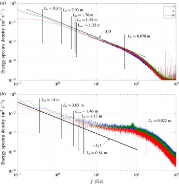
The high-resolution spectra (
 $T_{BR}=10~\text{s}$
) for no-burst/burst events of
 $\text{SI}_{out}$
are presented, respectively, in figures 12(a) and 12(b). While spectra for no-burst records exhibit the classical Kolmogorov shape (figure 12
a), the spectra with bursts strongly deviate from the Kolmogorov
 $-5/3$
shape for all three velocity components and exhibit a spectral ‘bump’ resembling a bottleneck effect, as discussed below.
A departure from the classical
 $k^{-5/3}$
spectra that leads to a shallower spectral slope, sometimes in the form of a bump, has been observed in many high-resolution numerical simulations of turbulence (Yeung & Zhou Reference Yeung and Zhou1997; Gotoh, Fukayama & Nakano Reference Gotoh, Fukayama and Nakano2002; Dobler et al.
Reference Dobler, Haugen, Yousef and Brandenburg2003; Kaneda et al.
Reference Kaneda, Ishihara, Yokokawa, Itakura and Uno2003; Mininni, Alexakis & Pouquet Reference Mininni, Alexakis and Pouquet2006; Donzis & Sreenivasan Reference Donzis and Sreenivasan2010) and experimental observations (She & Jackson Reference She and Jackson1993; Saddoughi & Veeravalli Reference Saddoughi and Veeravalli1994; Praskovsky & Oncley Reference Praskovsky and Oncley1997; Cerutti & Meneveau Reference Cerutti and Meneveau2000; Shen & Warhaft Reference Shen and Warhaft2000; Kit et al.
Reference Kit, Cherkassy, Saint and Fernando2010). These studies suggest that this bump disparity or bottleneck phenomenon arises due to dynamical effects that hinder the local downscale energy cascade, which is due to departure from the classical energy transfer mechanism from a given local wavenumber shell to its nearest neighbour. In the bottleneck case, significant interactions of the wavenumber in question with distant wavenumbers may exist (Verma & Donzis Reference Verma and Donzis2007). The energy cascade then becomes non-local, thus violating the assumptions of the Kolmogorov theory. In the present case, however, the spectral bumps appear to occur due to the bursts of unusual turbulence activity at small scales, sometimes encompassing the realm of the Taylor microscale. The effect on the larger scales appears to be insignificant compared to changes at smaller scales. While the exact mechanism responsible for burst generation and associated turbulence activities at high wavenumbers remains unclear, their effects on the structure of turbulence and TKE dissipation are definitely significant.
High-resolution spectra as in figure 9, but for
 $\text{SI}_{out}$
: (a) no-burst records and (b) burst records. The length scales are indicated by vertical lines. The total record is 420 s and was composed of 77 s of burst events and 343 s of no-burst events.

The resolved lower-frequency components also indicate that the spectral magnitudes of horizontal velocity components at low frequencies (figure 12 a) for the no-burst case are significantly higher (by one order) than that of the vertical velocity component, which is an upshot of stable stratification. The same tendency of the vertical velocity component magnitude being lower than that of the horizontal velocity component is preserved when bursting is present (figure 12 b), however to a lesser extent.
The developed and transitioning-out subintervals occurred about an hour after the initial transition from a strongly stratified (nominally laminar) flow regime. During the last 2 min of
 $\text{SI}_{out}$
, a similar flow transition was evident again with intense bursting, where both the mean and turbulent pulsations differ significantly from the typical values of the previous two subintervals. It is worth noting that after
 $\text{SI}_{out}$
the direction of the flow changed rapidly (not shown), whence the combo probe could not provide reliable data due to rapid wind variability.
3.4 Analysis of turbulence for developing flow
So far we have discussed significant bursting in developed flow regimes
 $\text{SI}_{devd}$
(
 $\text{SI}_{4}$
and first part of
 $\text{SI}_{5}$
). As figure 11 indicates, however, bursting is not unique to the developed flow regime and is also a characteristic of developing flow regimes. The developing stratified turbulence in
 $\text{SI}_{1}$
is characterized by extremely low TKE, which is more than one order lower than that in other subintervals, and even nominally laminar. There is a sharp transition at the beginning of
 $\text{SI}_{1}$
(22:00 MDT) from a highly variable flow to that characterized by a nearly constant wind direction (figure 2). Figure 13 shows the variation of
 $\unicode[STIX]{x1D700}$
in
 $\text{SI}_{1}$
(obtained using the same procedure as used for figures 5 and 6), which shows intermittent elevation of
 $\unicode[STIX]{x1D700}$
exceeding 20 times the background value.
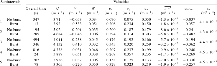
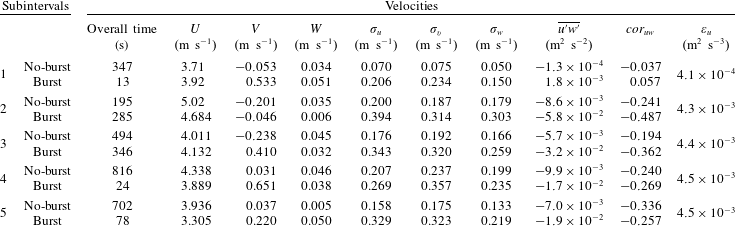
Figure 14 presents velocity fluctuations in a 10 s interval with a bursting event. These observations together with table 2 indicate that velocity fluctuations during no bursts are extremely low, becoming significant only during the bursts. Also, note that for
 $\text{SI}_{1}$
the MO scale is
 $L_{\ast }\approx 2{-}3~\text{m}$
, and hence in a statistical sense the processes at the combo level (
 $z=6~\text{m}$
) are dominated by buoyancy, decoupling it from surface shear and hence from possible vertical transport of turbulent events originating at the surface. This is supported by the small values of buoyancy
 $L_{b}$
(
 ${\sim}3~\text{m}$
) and vertical
 $L_{ver}$
(
 ${\sim}1~\text{m}$
) scales of stratified turbulence.
Time series of (a) block-averaged (1 s) kinetic energy dissipation rate
 $\unicode[STIX]{x1D700}$
for
 $SI_{1}$
(22:0122:07 MDT) and (b) flags separating burst/no-burst periods. The velocity fluctuations during a 10 s interval of the fourth minute (seconds 228–238 of the above record) are presented in figure 14.

Time series segment (10 s) of the velocity components of the fourth minute of
 $\text{SI}_{1}$
(22:01–22:07 MDT), showing intermittent high-frequency bursts.

As expected from the low TKE, the energy spectra of
 $\text{SI}_{1}$
are significantly lower and therefore stymied by noise (figure 15). Even in this developing case, the spectra for no-burst events exhibit an approximate Kolmogorov subrange. This may possibly be due to the slow time scale of flow evolution at the level of combos, which is
 $N^{-1}$
(
 ${>}$
10 s); hence in the time intervals considered for analysis (
 ${\leqslant}$
10 s), the turbulence behaves as if the flow is quasi-stationary. Bursting events lead to spectral bumps as in other subintervals.
Energy spectral density of velocity components in
 $\text{SI}_{1}$
computed at high resolution
 $\unicode[STIX]{x0394}f=0.1~\text{Hz}$
(22:01–22:07 MDT): (a) no-burst records and (b) burst records. The length scales are indicated by vertical lines. The total record lasted 360 s and was composed of 13 s of burst events and 347 s of no-burst events.

The
 $\text{SI}_{2}$
immediately follows
 $\text{SI}_{1}$
, and strong increase of TKE (figure 4) hints at fast flow development that helps transition to a developed turbulent flow. Thus,
 $\text{SI}_{2}$
contains more bursting than no-bursting events, some of which are extremely strong (see figure 16 and table 2). The high-resolution spectra of
 $\text{SI}_{2}$
combined with
 $\text{SI}_{3}$
(dubbed transitioning-in time period) are presented in figures 17(a) and 17(b), respectively, for no-burst and burst records. They clearly demonstrate that: (i) the spectral densities of the vertical velocity at low frequencies are almost an order smaller than those of longitudinal velocity components, as expected due to stratification; and (ii) the spectral shape without bursting is of clear Kolmogorov type while those with bursting events show a striking spectral bump.
Time series of (a) kinetic energy dissipation rate and (b) flag separating burst/no-burst time intervals for combined transitioning-in time interval comprising
 $\text{SI}_{2}$
and
 $\text{SI}_{3}$
(22:09–22:32 MDT).

Energy spectral density computed with high resolution
 $\unicode[STIX]{x0394}f=0.1~\text{Hz}$
for combined transitioning-in time interval comprising
 $\text{SI}_{2}$
and
 $\text{SI}_{3}$
: (a) no-burst and (b) burst records. The length scales are indicated by vertical lines. The total record is 1320 s, composed of 631 s of bursts and 689 s of no-burst events.

Because of the non-compliance of thresholds used for accepting data from the combo for in situ calibration (i.e. alignment of probe and wind vector better that
 $10^{\circ }$
for each minute during five consecutive minutes, which are necessary to construct a training set for the NN calibration algorithm), no reliable data could be obtained in the interval between the end of
 $\text{SI}_{3}$
and the beginning of
 $\text{SI}_{4}$
. Fortunately, the turbulence parameters were very stable during
 $\text{SI}_{devd}$
for obtaining reliable information on stationary stratified shear flows.
3.5 Summary of flow parameters inside burst/no-burst events within all subintervals
In table 2, the mean and r.m.s. velocities of all three components for burst/no-burst events in different subintervals are presented together with the background dissipation rate
 $\unicode[STIX]{x1D700}$
and the normalized correlation coefficient
 $cor_{uw}=\langle (u-U)(w-W)\rangle /\unicode[STIX]{x1D70E}_{u}\unicode[STIX]{x1D70E}_{w}$
between the longitudinal and vertical velocity components, the latter being related to the Reynolds stresses responsible for TKE production. In
 $\text{SI}_{1}$
,
 $\text{SI}_{4}$
and
 $\text{SI}_{5}$
, no-burst events are the most common, while burst and no-burst events are roughly of similar durations in
 $\text{SI}_{2}$
and
 $\text{SI}_{3}$
. In
 $\text{SI}_{2}$
, the duration of burst events exceeds the no-burst events, while the opposite holds for
 $\text{SI}_{3}$
.
In all subintervals, during both bursting and no-bursting events, the mean vertical velocity was very low, typically positive (upwards) as could be expected in the boundary layer, and was approximately 1 % of the mean wind velocity (thus the values are teetering at the permissible resolution of measurements). Bursting can change the horizontal mean velocity vector slightly, as they cause small variations of streamwise and lateral mean velocity components. The r.m.s. values change noticeably during bursts, showing a significant change of TKE. The effect of bursting on the Reynolds stresses is not as clear, but generally there is a discernible increase while the correlation coefficient
 $cor_{uw}$
, varies in the range
 $-0.2$
to
 $-0.4$
for both burst and no-burst cases, in all subintervals except in
 $\text{SI}_{1}$
(see table 2). During
 $\text{SI}_{1}$
(figure 4
a), the mean longitudinal velocity is approximately
 $3.7~\text{m}~\text{s}^{-1}$
, the other two components being low. During the same period, the normalized (by
 $U$
) r.m.s. velocities in the direction of the wind and in the vertical direction are
 ${<}$
2 % and
 ${<}$
1.5 %, respectively, which are very low compared to the typical values of 5 % in other subintervals. The spectral shape is close to
 $k^{-5/3}$
followed by a fall-off when no-burst periods are used for calculations (figure 15
a), but deviations are evident when bursts are present (figure 15
b).
Mean and r.m.s. velocities along with the normalized Reynolds stress for burst/no-burst events obtained during the five subintervals comprising the initial period of flow regime transition.
4 Discussion and concluding remarks
Following Kit et al. (Reference Kit, Cherkassy, Saint and Fernando2010), a combo-probe system that consists of a multi-sensor hot-film probe co-located with a sonic anemometer (sonic) was developed, with the latter calibrating the former using a neural network (NN) based on data obtained simultaneously by the two probes with different space-time resolutions. Sonics are commonly used in atmospheric research, but low space-time resolution limits their utility in probing fine-scale turbulence. Hot-film/wire probes may provide velocity information down to dissipation scales, but require frequent and laborious calibrations as well as specific alignment of probes relative to the flow. A combo system circumvents such difficulties by automatically adjusting the hot-film probes to the wind direction, guided by in situ data provided by sonic. The sonic data are also used by the NN for calibration and to align the hot-film probe to the mean wind direction via a precision stepper motor and a feedback control system. This arrangement enabled sampling of turbulence during the MATERHORN field experiments without interruption for several days at a time. Since only
 $120^{\circ }$
sectors were accessible with the type of sonics used, not all of the data were of utility but there were significant time intervals over which high-quality data were available. The interpretation of data in the context of fundamental theories and concepts, however, was fraught with problems due to the complexity of the flow (e.g. directional shear, rapid evolution).
In the present study, almost 90 min of remarkably high-quality data taken from a 32 m flux tower, during a period where the flow transitioned from a nominally quiescent flow regime to a fully developed turbulence regime, were analysed. Identification of this transition at the tower was consistent with large-scale (synoptic) flow observations during MATERHORN. The analysis period started at 22:00 MDT (local time) on 19 October 2012. The local gradient Richardson number over the entire 90 min period was in the proximity of the critical value of 0.25 except at the beginning (figure 3), and hence both the shear production and buoyancy effects appear to be important. As such, the analysis period was ideal for stratified parallel shear flow studies, where the flow is capable of achieving statistical equilibrium, balancing shear production, dissipation and buoyancy flux. Within the above period, five subintervals (
 $\text{SI}_{1}{-}\text{SI}_{5}$
) were identified based on the nature of turbulence statistics.
 $\text{SI}_{1}$
was nominally laminar,
 $\text{SI}_{2}$
and
 $\text{SI}_{3}$
resembled a rapid flow developing state (also combined to call the transitioning-in regime
 $\text{SI}_{tr\text{-}in}$
),
 $\text{SI}_{4}$
and the first part of
 $\text{SI}_{5}$
represented a fully developed equilibrium state (
 $\text{SI}_{devd}$
) and the last part of
 $\text{SI}_{5}$
represented still another rapidly growing or transitioning-out regime (
 $\text{SI}_{out}$
).
During data processing and analyses a new phenomenon was identified: strong intermittent bursting with intense fluctuations occurring at small scales (0.1–0.4 m) that are unaffected by stratification, although large scales feel stratification effects. A post-processing procedure was developed that separates time series into burst and no-burst periods within a given subinterval. The latter exhibited classical Kolmogorov spectra, while periods with bursts led to spectra with bottleneck behaviour signified by a spectral bump. Past work on the bottleneck effect suggest the involvement of viscous effects (Falkovich Reference Falkovich1994; Verma & Donzis Reference Verma and Donzis2007) or buoyancy effects (Waite Reference Waite2011; Augier, Galtier & Billant Reference Augier, Galtier and Billant2012) in modifying the local energy cascade to facilitate non-local effects, but our results were not consistent with these proposals. That is, the humps did not consistently appear near the Taylor microscale or the buoyancy scale. Conversely, the spectra tended to roll off near the Taylor microscale for no-burst cases, indicating the onset of viscous effects. When bursts are present, the viscous roll-off did not occur consistently at the Taylor scale, indicating the possible importance of bursts in scaling the dissipation regime.
During other time intervals of the autumn 2012 MATERHORN campaign, in particular, during transition periods from unstable to stable periods and vice versa, bursting events have been observed in hot-film data. Bursting was also observed during stable and transition periods of the spring 2013 campaign. Unfortunately, there are difficulties with the use of these data due to problems that plagued the sonic measurements, which are necessary in the NN approach of combo-probe calibration, as well as complexity of the flow (non-parallel nature). Most other field campaigns have not employed the new combo-probe technology to observe strong fine-scale bursting. In addition, the data mining is a very delicate process and phenomena of this ilk can be easily overlooked. In particular, the appearance of significant but relatively short bursts of velocity fluctuations embedded in otherwise uneventful data did not catch our attention until it was noticed that such bursts consistently appeared in one of the subintervals. Thereafter, all the data were carefully screened and similar behaviour was unravelled in other time intervals with varying degrees of manifestation.
Computation of velocity derivative skewness demonstrated that for the developed regime (
 $\text{SI}_{4}$
) the skewness oscillated around
 $-0.4$
when bursts are absent. When bursts are present, the skewness strongly fluctuates with a mean other than
 $-0.4$
, and it can even become positive during some bursting events (figure 10). This suggests the possible emergence of new small-scale dynamics akin to bursting that does not follow classical concepts of enstrophy generation and cascade.
The normalized correlation coefficient between longitudinal and vertical velocity components (see table 2), which is related to TKE production by the interactions of Reynolds stresses and mean shear, was calculated separately for bursting and no-bursting events. Very similar values of correlation coefficients were obtained (in the range
 $-0.4$
to
 $-0.2$
), thus suggesting that turbulence generated within bursting events has similarities with typical shear-produced turbulence (though production may follow different dynamics and its value during bursting is higher due to higher r.m.s. of both velocity components). This is quite remarkable, since it shows that Reynolds stresses are of importance both with and without bursts. This bolsters the notion that the signals are of real turbulent nature and not caused by background electromagnetic or mechanical noise.
Characteristic length scales were calculated and placed alongside the energy spectral density plots. Theoretical work suggests that for stationary flows the Ozmidov scale
 $L_{O}$
separates the spectral regions affected by stratification from the isotropic Kolmogorov regime (e.g. Riley & Lindborg Reference Riley and Lindborg2008). The buoyancy scale
 $L_{b}$
is assumed to demarcate larger horizontal scales from the region where vertical motions are constrained but horizontal motions of scales
 $L_{h}$
are unaffected by stratification. Thus, in
 $L_{O}<2\unicode[STIX]{x03C0}/k<L_{h}$
, three-dimensional inertial energy cascading and hence a
 $k^{-5/3}$
regime is possible in the horizontal velocity spectrum, but not in the vertical one; scales smaller than
 $L_{O}~({<}L_{b})$
were suggested to exhibit isotropic behaviour. Our results for stationary cases (
 $\text{SI}_{devd}$
) indeed are consistent with these proposals, although for non-stationary cases glaring inconsistencies are evident. The spectral anisotropy appears at scales larger than
 $L_{ver}$
, which is smaller than
 $L_{b}$
in all cases.
While the mechanism underlying burst generation could not be delineated by our work due to lack of background spatial data that could be used in conjunction with hot-film events, the bursts described here differ from the sporadic turbulence events reported in the literature that date back to Durst (Reference Durst1933); they are instabilities such as Kelvin–Helmholtz billowing that intermittently feed energy at vertical scales
 ${\sim}L_{b}$
. The bursts in our case occur at smaller scales (
 ${<}L_{b}$
) than those that could be resolved by the sonics. Bursts produce sufficient energy to form a spectral bump, augmenting the usual cascade that drives much smaller
 $\unicode[STIX]{x1D700}$
compared to that corresponding to bursts. This poses challenges to dissipation (EDR) estimates in practical applications based on the Kolmogorov inertial subrange, as additional production may occur at still smaller scales.
A plausible mechanism for bursts is the critical layer absorption of small-scale internal waves in stratified shear flows, which spasmodically produces small-scale turbulence by local convective overturning instabilities (Koop Reference Koop1981). The wavenumber at the onset of the spectral bump (except in a few cases) scales well with the local shear length scale
 $L_{S}$
, which is broadly consistent with the internal-wave/shear interaction notion. The downward transport of patchy turbulent regions, generated in a low-level jet, such as in Ohya et al. (Reference Ohya, Nakamura and Uchida2008), is another possibility, as is the reaching of upward-moving boundary layer bursts (Kline et al.
Reference Kline, Reynolds, Schraub and Runstadler1967; Rao, Narasimha & Narayanan Reference Rao, Narasimha and Narayanan1971) to the level of the combo probe. The Monin–Obukhov length scales computed for developing (
 $\text{SI}_{tr\text{-}in}$
) and developed (
 $\text{SI}_{devd}$
) subintervals show that both alternatives are also plausible since buoyancy and surface shear are of equal importance at the combo height. The calculations of vertical kinetic energy flux (not shown) at the combo level, nonetheless, did not support the notion that bursts are disturbances arriving from the ground or aloft. Also note that the disturbances are advected past the hot-film probe, and hence they could be generated elsewhere and remain active while passing the probe.
Given the observational difficulties in the field, many outstanding questions remain with regard to burst generation: (i) Is small-scale bursting in the SBL a characteristic of complex terrain? – No field or laboratory measurements exist in flat terrain to the detail reported herein to address this issue, although Ohya et al. (Reference Ohya, Nakamura and Uchida2008) reported bursts in flat terrain weakly stratified laboratory boundary layers without delineating the scales involved. (ii) Are bursts of this ilk characteristic of very stable, convective and neutral boundary layers? – The present data have been taken in the proximity of the critical Richardson number, in a moderately stratified regime. The limited observations of Kit et al. (Reference Kit, Cherkassy, Saint and Fernando2010) indicate that convective boundary layers are devoid of such bursts. (iii) What is the mechanism of burst generation? – Bursting reported in our study has much stronger dissipation rates than those of the intermittent turbulence events described in previous studies, for example, in global (large-scale patches) and small-scale (velocity gradient organized by individual eddies) intermittencies discussed by Mahrt (Reference Mahrt1989) and Sreenivasan & Antonia (Reference Sreenivasan and Antonia1997). To address such issues, a field campaign with comprehensive characterization of background flow (suitably spaced flux towers and energy balance stations to evaluate profiles and energetics) and high-resolution measurement of local flow (hot-film anemometry and high space-time resolution thermistors for point velocity, temperature and flux measurements as well as holographic particle image velocity for space-time measurements) are needed to resolve three-dimensional sub-metre-scale wave, shear and turbulence processes. We believe that field campaigns as well as laboratory and numerical studies dealing with bursting phenomena are of value for the benefit of understanding small-scale dynamics of geophysical boundary layers, wherein the fluxes are dominant and most of the TKE dissipation takes place. Field studies are of particular value as they encompass natural complexities and have Reynolds numbers close to those assumed in classical turbulence theories. With recent advances of measurement technologies, such field studies are now feasible, though they demand intensive technical, logistical and financial resources.
Acknowledgements
The results presented were obtained during the MATERHORN programme that was funded by the Office of Naval Research Award No. N00014-11-1-0709. We thank Professor Y. Ohya for his support. Dr P. Conry provided valuable assistance in additional data processing and double-checking. Dr S. Oncley of NCAR provided valuable hardware support for the combo project. E.K. and D.L. were also supported by the Israel Science Foundation (Grants 426/12 and 408/15). During the analysis period, H.J.S.F. was funded by NSF grants AGS-1528451 and AGS-1565535. We are indebted to three anonymous reviewers for their valuable and insightful comments and for challenging us with comprehensive questions, the addressing of which without doubt significantly improved the content of the manuscript and its readability.