1 Introduction
Various physical processes arising in a rotating stratified fluid are largely explained in terms of wave dynamics. Waves generated by external, or sometimes internal, forcing propagate spatially in a fluid, transporting momentum and energy, which are fundamental ingredients of the large-scale steady motions in the atmosphere (Yiğit & Medvedev Reference Yiğit and Medvedev2015) and the ocean (MacKinnon et al. Reference MacKinnon, Zhao, Whalen, Waterhouse, Trossman, Sun, Laurent, Simmons, Polzin and Pinkel2017). Over the last couple of decades, owing to the development of computational power, more and more accurate numerical simulation systems have been developed to reproduce the interaction between the mean state and fluctuating waves in the atmosphere and ocean. Accordingly, extraction of wave signals from the model output data that involve physical variables such as velocity, density and pressure, and evaluation of their impacts on the larger-scale flow field have become increasingly important tasks. For this purpose, advanced diagnostic tools have been invented to illustrate the geography of the wave properties, such as energy, momentum and their fluxes.
A series of studies, such as those of Plumb (Reference Plumb1985), Takaya & Nakamura (Reference Takaya and Nakamura1997), Takaya & Nakamura (Reference Takaya and Nakamura2001), Kinoshita, Tomikawa & Sato (Reference Kinoshita, Tomikawa and Sato2010) and Kinoshita & Sato (Reference Kinoshita and Sato2013), provide examples in which the pseudo-momentum flux associated with Rossby waves (RWs) and inertia–gravity waves (IGWs) is formulated so as to be calculable using data obtained from general atmospheric models. An assumption underlying these methods is that spatial variation in the medium is much slower than the wave oscillation, so that all of the variables can be locally decomposable into plane monochromatic components, which are solutions of linear equations with constant coefficients. This scale separation assumption is frequently referred to as the Wentzel–Kramers–Brillouin–Jeffreys (WKBJ) approximation. The original WKBJ theory is, however, merely a solution method for differential equations (Bender & Orszag Reference Bender and Orszag1999). For data diagnostic purposes, instead of a solution, deriving a conservation equation in the form of
 $$\begin{eqnarray}\frac{\unicode[STIX]{x2202}A}{\unicode[STIX]{x2202}t}+\unicode[STIX]{x1D735}\boldsymbol{\cdot }\boldsymbol{F}=S,\end{eqnarray}$$
and numerically computing  $\boldsymbol{F}$ are the central objectives (see, e.g. Takaya & Nakamura Reference Takaya and Nakamura2001). Here
 $A$,
 $\boldsymbol{F}$ and
 $S$ are the energy or pseudo-momentum density, its flux and the source or sink term, respectively. In the limit of a monochromatic wave train,
 $\boldsymbol{F}$ should be reduced to the product of
 $A$ and the group velocity. To ensure this property is sometimes a difficult task (Aiki, Greatbatch & Claus Reference Aiki, Greatbatch and Claus2017).
The background underlying this flux analysis is the transport theory (Ryzhik, Papanicolaou & Keller Reference Ryzhik, Papanicolaou and Keller1996; Guo & Wang Reference Guo and Wang1999, and references therein). In this theory, the density of some conserved quantity is defined in physical and wavenumber space and its transfer is described by the transport equation,
 $$\begin{eqnarray}\frac{\unicode[STIX]{x2202}w}{\unicode[STIX]{x2202}t}+\unicode[STIX]{x1D735}_{x}\boldsymbol{\cdot }(w\unicode[STIX]{x1D735}_{k}\unicode[STIX]{x1D714})-\unicode[STIX]{x1D735}_{k}\boldsymbol{\cdot }(w\unicode[STIX]{x1D735}_{x}\unicode[STIX]{x1D714})=s,\end{eqnarray}$$
where  $w(\boldsymbol{x},\boldsymbol{k},t)$ is the density of a conserved quantity,
 $\unicode[STIX]{x1D714}(\boldsymbol{x},\boldsymbol{k})$ is the dispersion relation,
 $\unicode[STIX]{x1D735}_{x}$ and
 $\unicode[STIX]{x1D735}_{k}$ are gradients in physical and wavenumber space, respectively, and
 $s$ represents source, decay and scattering effect. In this theory, wavenumber
 $\boldsymbol{k}$ is defined in a quasi-local sense:
 $(\boldsymbol{x},\boldsymbol{k})$ specifies a wave packet with a local wavenumber
 $\boldsymbol{k}$ located in the vicinity of
 $\boldsymbol{x}$. The characteristics of (1.2) are specified by a set of equations,
 $\dot{\boldsymbol{x}}=\unicode[STIX]{x1D735}_{k}\unicode[STIX]{x1D714}$ and
 $\dot{\boldsymbol{k}}=-\unicode[STIX]{x1D735}_{x}\unicode[STIX]{x1D714}$, which represents the wave trajectory in physical and wavenumber space, and solving these equations is referred to as ray tracing (Lighthill Reference Lighthill1978). When (1.2) is integrated in wavenumber space, the usual conservation equation (1.1) is derived.
The transport equation (1.2) is operationally used to predict the ocean surface state in the numerical models developed, such as that by WAMDI Group (1988). As for geophysical fluid dynamics, transport theory has been developed by Powell & Vanneste (Reference Powell and Vanneste2005), Wordsworth (Reference Wordsworth2009), Danioux & Vanneste (Reference Danioux and Vanneste2016), Savva & Vanneste (Reference Savva and Vanneste2018) and Kafiabad, Savva & Vanneste (Reference Kafiabad, Savva and Vanneste2019). In recent years, the transport equation (1.2) has also been incorporated into the prediction systems for the ocean interior (Olbers & Eden Reference Olbers and Eden2013; Eden & Olbers Reference Eden and Olbers2017).
The aim of the current study is, however, neither to investigate a specific process using the transport theory nor to develop a numerical method to integrate the transport equation. Instead, the transport theory is here utilised for data diagnostic purposes. More specifically, this paper explores the method to compute the terms in the transport equation (1.2) using data produced from a common numerical model. A challenge in this work is to decompose different modes in a spatially varying medium.
In a rotating stratified fluid with the Boussinesq approximation, an arbitrary infinitesimal motion is regarded as a superposition of rapidly oscillating IGWs, sometimes called the wave mode, and the quasi-stationary vortical mode. If the coefficient parameters of the equations of motion, such as the Brunt–Väisälä frequency, the Coriolis parameter and the background mean velocity, are spatially constant, the two distinct modes can be clearly decomposed by taking the Fourier transform and projecting the variables onto the eigenvectors of the coefficient matrix of the equations. This eigenvector is called the polarisation relation and specifies the kinematic characteristics of each mode: the oscillation angle or the relative phases and amplitudes of the variables. The homogeneous wave–vortex decomposition technique has been frequently used to analyse flow field data (e.g. Lien & Müller Reference Lien and Müller1992; Bühler, Callies & Ferrari Reference Bühler, Callies and Ferrari2014; Bühler, Kuang & Tabak Reference Bühler, Kuang and Tabak2017). If the system is inhomogeneous due to variations in coefficient parameters, the polarisation relations of both the wave and vortical modes vary from place to place so that the usual Fourier analysis becomes ineffective.
The difficulty is not only in the variations in the polarisation relations. The local dispersion relation of each mode is also modified due to the effect of gradients in parameters. For example, the gradient in the background potential vorticity due to the planetary  $\unicode[STIX]{x1D6FD}$-effect (
 $\unicode[STIX]{x1D6FD}$ represents the meridional variation in the Coriolis parameter) or topographic slope causes the vortical modes to oscillate as RWs. The gradient in the background flow velocity modifies the dispersion relation of IGWs, which substantially affects the propagation of near-inertial waves in a frontal area (Kunze Reference Kunze1985). The frequency shift due to inhomogeneity is explained by the WKBJ method when the higher-order terms in the phase of variables, which are called geometric phase, are analysed. In geophysical fluid dynamics, this phase shift has been considered for example by Bretherton (Reference Bretherton1968) and Vanneste & Shepherd (Reference Vanneste and Shepherd1999), and even made explicit by McKee (Reference McKee1973), but is commonly ignored in ray-tracing methods (Bühler Reference Bühler2014). Although Guo & Wang (Reference Guo and Wang1999) and Powell & Vanneste (Reference Powell and Vanneste2005) formulated a procedure to separately derive the transport equation for each mode in an inhomogeneous medium, their methods are still insufficient to incorporate the effect of the frequency shift.
To overcome the problems raised above, this study develops theoretical and numerical methods of wave decomposition properly taking account of the inhomogeneity of the system. The plan of this paper is as follows. In § 2, we discuss a general description of wave motions in an inviscid fluid system in terms of Wigner transform, which enables a set of simultaneous wave equations to be asymptotically decomposed into the ones governing mutually independent modes. Defining the Wigner distribution function, we subsequently derive the transport equation. In § 3, we take an example of a rotating shallow water model, in which variations in the Coriolis parameter and the depth cause slow propagation of the vortical mode as RWs. We confirm that the present method appropriately derives the dispersion relation of the RWs in a perturbation term, and therefore their propagation is well described in this framework. A simple numerical experiment is also conducted, which demonstrates the usefulness of this method for the diagnosis of model data. Discussion and conclusions are presented in § 4.
2 General description of wave decomposition and transport theory
2.1 Linear waves in a non-canonical Hamiltonian system
Since the purpose of this study is to offer a methodology of wave decomposition applicable to a wide variety of fluid systems, we begin with a mathematical description of fluid motion in its most general form. According to Morrison (Reference Morrison1998), evolution equations for an inviscid fluid are written in a non-canonical Hamiltonian form,
 $$\begin{eqnarray}\displaystyle \frac{\unicode[STIX]{x2202}\unicode[STIX]{x1D74A}}{\unicode[STIX]{x2202}t}=\hat{\unicode[STIX]{x1D645}}(\unicode[STIX]{x1D74A})\frac{\unicode[STIX]{x1D6FF}{\mathcal{H}}}{\unicode[STIX]{x1D6FF}\unicode[STIX]{x1D74A}}, & & \displaystyle\end{eqnarray}$$
where the state vector  $\unicode[STIX]{x1D74A}(\boldsymbol{x},t):\mathbb{R}^{d+1}\rightarrow \mathbb{R}^{n}$ represents physical variables such as velocity or spatial displacement of the medium,
 $\hat{\unicode[STIX]{x1D645}}(\unicode[STIX]{x1D74A})$ is a nonlinear skew-Hermitian operator and
 ${\mathcal{H}}[\unicode[STIX]{x1D74A}]$ is a Hamiltonian functional generally consisting of the energy and some Casimir invariants. Assuming an infinitesimal fluctuation from a local minimum point of
 ${\mathcal{H}}$, which we write
 $\unicode[STIX]{x1D74A}=\unicode[STIX]{x1D730}+\unicode[STIX]{x1D74A}^{\prime }$, the governing equation (2.1) becomes
 $$\begin{eqnarray}\displaystyle \frac{\unicode[STIX]{x2202}\unicode[STIX]{x1D74A}^{\prime }}{\unicode[STIX]{x2202}t}=\hat{\unicode[STIX]{x1D645}}(\unicode[STIX]{x1D730})\left.\frac{\unicode[STIX]{x1D6FF}^{2}{\mathcal{H}}}{\unicode[STIX]{x1D6FF}\unicode[STIX]{x1D74A}^{2}}\right|_{\unicode[STIX]{x1D730}}\unicode[STIX]{x1D74A}^{\prime }. & & \displaystyle\end{eqnarray}$$
Then, extending the definition of state vectors from real to complex variables and defining linear Hermitian operators,  $\unicode[STIX]{x1D6FF}^{2}{\mathcal{H}}/\unicode[STIX]{x1D6FF}\unicode[STIX]{x1D74A}^{2}|_{\unicode[STIX]{x1D730}}\equiv \hat{\unicode[STIX]{x1D63C}}$ and
 $\text{i}\hat{\unicode[STIX]{x1D63C}}\hat{\unicode[STIX]{x1D645}}(\unicode[STIX]{x1D730})\hat{\unicode[STIX]{x1D63C}}\equiv \hat{\unicode[STIX]{x1D63D}}$, we rewrite (2.2) as
 $$\begin{eqnarray}\displaystyle \text{i}\hat{\unicode[STIX]{x1D63C}}\frac{\unicode[STIX]{x2202}\unicode[STIX]{x1D74A}^{\prime }}{\unicode[STIX]{x2202}t}=\hat{\unicode[STIX]{x1D63D}}\unicode[STIX]{x1D74A}^{\prime }. & & \displaystyle\end{eqnarray}$$
In the following,  $^{\dagger }$ denotes the complex conjugate. According to (2.3), the functional
 ${\mathcal{E}}[\unicode[STIX]{x1D74A}^{\prime }]\equiv (1/2)\int \unicode[STIX]{x1D74A}^{\prime \dagger }\hat{\unicode[STIX]{x1D63C}}\unicode[STIX]{x1D74A}^{\prime }\text{d}\boldsymbol{x}$ remains unchanged with time:
 $\text{d}{\mathcal{E}}/\text{d}t=0$. This functional is related to
 ${\mathcal{H}}$ as
 ${\mathcal{H}}[\unicode[STIX]{x1D730}+\unicode[STIX]{x1D74A}^{\prime }]-{\mathcal{H}}[\unicode[STIX]{x1D730}]={\mathcal{E}}[\unicode[STIX]{x1D74A}^{\prime }]+O(|\unicode[STIX]{x1D74A}^{\prime }|^{3})$. In this study, we regard
 ${\mathcal{E}}$ as the total wave energy of the system. It is noted that, when discussing wave–mean flow interaction processes, the total pseudoenergy, pseudo-momentum or wave action would be a more suitable choice as the invariant of the system. In any case, our analysis does not depend on the physical meaning of
 ${\mathcal{E}}$ so long as the system is governed by an equation written as (2.3). Please refer to Shepherd (Reference Shepherd1990) for the non-canonical Hamiltonian formulation (2.1) of various problems arising in geophysical fluid dynamics.
To simplify the problem, we have assumed that the reference state  $\unicode[STIX]{x1D730}$ is the local minimum point of the Hamiltonian functional
 ${\mathcal{H}}$, which makes
 $\hat{\unicode[STIX]{x1D63C}}$ positive–definite. This is the necessary condition for
 ${\mathcal{E}}\geqslant 0$ and also a sufficient condition for the stability of the system (Shepherd Reference Shepherd1990). Then, in the same way as the usual matrix calculation, we consider a factorisation of
 $\hat{\unicode[STIX]{x1D63C}}$; that is, we seek an operator
 $\hat{\unicode[STIX]{x1D647}}$ that satisfies
 $$\begin{eqnarray}\displaystyle \hat{\unicode[STIX]{x1D63C}}=\hat{\unicode[STIX]{x1D647}}\hat{\unicode[STIX]{x1D647}}^{\dagger }. & & \displaystyle\end{eqnarray}$$
Let us suppose that this factorisation is achieved and, in addition, we find an inverse of  $\hat{\unicode[STIX]{x1D647}}$; namely,
 $\hat{\unicode[STIX]{x1D647}}^{-1}$ that satisfies
 $\hat{\unicode[STIX]{x1D647}}\hat{\unicode[STIX]{x1D647}}^{-1}=\hat{\unicode[STIX]{x1D647}}^{-1}\hat{\unicode[STIX]{x1D647}}=\hat{\boldsymbol{I}}$ where
 $\hat{\boldsymbol{I}}$ is the identity operator. Then, redefining the state vector and the Hermitian operator as
 $\unicode[STIX]{x1D74D}=\hat{\unicode[STIX]{x1D647}}^{\dagger }\unicode[STIX]{x1D74A}^{\prime }/\sqrt{2}$ and
 $\hat{\unicode[STIX]{x1D643}}=\hat{\unicode[STIX]{x1D647}}^{-1}\hat{\unicode[STIX]{x1D63D}}\hat{\unicode[STIX]{x1D647}}^{\dagger -1}$, we may further simplify (2.3) as
 $$\begin{eqnarray}\displaystyle \text{i}\frac{\unicode[STIX]{x2202}\unicode[STIX]{x1D74D}}{\unicode[STIX]{x2202}t}=\hat{\unicode[STIX]{x1D643}}\unicode[STIX]{x1D74D}, & & \displaystyle\end{eqnarray}$$
which is the most basic description for a linear system that conserves the energy norm  ${\mathcal{E}}=\int |\unicode[STIX]{x1D74D}|^{2}\,\text{d}\boldsymbol{x}$.
2.2 Wigner transform and pseudo-differential operator
To seek an operator  $\hat{\unicode[STIX]{x1D647}}$ that satisfies the condition (2.4), here we use the Wigner transform. The Wigner transform is a kind of mapping that associates a linear operator with a function called the symbol, which is frequently used in theoretical physics to correspond a quantum system to a classical system (e.g. McDonald Reference McDonald1988; Gérard et al. Reference Gérard, Markowich, Mauser and Poupaud1997; Cohen Reference Cohen2012). When an operator acting on functional space is given, its Wigner transform is defined as follows: we first represent the operator in an integral transformation form,
 $$\begin{eqnarray}\hat{\unicode[STIX]{x1D641}}\unicode[STIX]{x1D753}(\boldsymbol{x})=\int \unicode[STIX]{x1D641}(\boldsymbol{x},\boldsymbol{x}^{\prime })\unicode[STIX]{x1D753}(\boldsymbol{x}^{\prime })\,\text{d}\boldsymbol{x}^{\prime },\end{eqnarray}$$
where  $\unicode[STIX]{x1D753}(\boldsymbol{x}):\mathbb{R}^{d}\rightarrow \mathbb{C}^{n}$ is an arbitrary test function. Then, the Fourier transform of the kernel function with respect to the relative position of its arguments yields the symbol,
 $$\begin{eqnarray}\unicode[STIX]{x1D65B}(\boldsymbol{x},\boldsymbol{p})=\int \unicode[STIX]{x1D641}\left(\boldsymbol{x}+\frac{\boldsymbol{x}^{\prime }}{2},\boldsymbol{x}-\frac{\boldsymbol{x}^{\prime }}{2}\right)\text{e}^{-\text{i}\boldsymbol{p}\boldsymbol{\cdot }\boldsymbol{x}^{\prime }/\unicode[STIX]{x1D707}}\,\text{d}\boldsymbol{x}^{\prime },\end{eqnarray}$$
where the parameter  $\unicode[STIX]{x1D707}$, which corresponds to the Dirac constant in quantum mechanics, is introduced. Wavenumber is now represented by
 $\boldsymbol{p}$, which is distinguished from the usual definition
 $\boldsymbol{k}$ by a multiplication factor
 $\unicode[STIX]{x1D707}$; i.e. one may understand that a relationship
 $\boldsymbol{p}=\unicode[STIX]{x1D707}\boldsymbol{k}$ holds. A symbol is a matrix-valued function defined on
 $\mathbb{R}^{2d}$. The operator
 $\hat{\unicode[STIX]{x1D641}}$ is then represented using its symbol
 $\unicode[STIX]{x1D65B}(\boldsymbol{x},\boldsymbol{p})$ as a kind of pseudo-differential operator,
 $$\begin{eqnarray}\hat{\unicode[STIX]{x1D641}}\unicode[STIX]{x1D753}(\boldsymbol{x})=\frac{1}{(2\unicode[STIX]{x03C0}\unicode[STIX]{x1D707})^{d}}\iint \unicode[STIX]{x1D65B}\left(\frac{\boldsymbol{x}+\boldsymbol{x}^{\prime }}{2},\boldsymbol{p}\right)\unicode[STIX]{x1D753}(\boldsymbol{x}^{\prime })\text{e}^{\text{i}\boldsymbol{p}\boldsymbol{\cdot }(\boldsymbol{x}-\boldsymbol{x}^{\prime })/\unicode[STIX]{x1D707}}\,\text{d}\boldsymbol{x}^{\prime }\,\text{d}\boldsymbol{p},\end{eqnarray}$$
which is rather simply denoted as  $\hat{\unicode[STIX]{x1D641}}=\unicode[STIX]{x1D65B}(\hat{\boldsymbol{x}},\hat{\boldsymbol{p}})$. It is noted that, whereas the mapping from an operator to a function,
 $\hat{\unicode[STIX]{x1D641}}\rightarrow \unicode[STIX]{x1D65B}(\boldsymbol{x},\boldsymbol{p})$, is called the Wigner transform, its inverse,
 $\unicode[STIX]{x1D65B}(\boldsymbol{x},\boldsymbol{p})\rightarrow \hat{\unicode[STIX]{x1D641}}$, is called the Weyl correspondence. In this study, we assume that
 $\unicode[STIX]{x1D707}\ll 1$ and all the symbols can be expanded in terms of
 $\unicode[STIX]{x1D707}$; such as
 $$\begin{eqnarray}\unicode[STIX]{x1D65B}=\unicode[STIX]{x1D65B}_{0}+\unicode[STIX]{x1D707}\unicode[STIX]{x1D65B}_{1}+\unicode[STIX]{x1D707}^{2}\unicode[STIX]{x1D65B}_{2}+\cdots \,,\end{eqnarray}$$
which are the same requirements as those for the usual WKBJ approximation.
The Wigner transform associates a product between operators,  $\hat{\unicode[STIX]{x1D641}}\hat{\unicode[STIX]{x1D642}}=\unicode[STIX]{x1D65B}(\hat{\boldsymbol{x}},\hat{\boldsymbol{p}})\unicode[STIX]{x1D65C}(\hat{\boldsymbol{x}},\hat{\boldsymbol{p}})$, with an operation between their symbols, which is called the star product and denoted as
 $\unicode[STIX]{x1D65B}(\boldsymbol{x},\boldsymbol{p})\star \unicode[STIX]{x1D65C}(\boldsymbol{x},\boldsymbol{p})$. As described in appendix A, we may explicitly expand the definition of the star product as follows:
 $$\begin{eqnarray}\unicode[STIX]{x1D65B}(\boldsymbol{x},\boldsymbol{p})\star \unicode[STIX]{x1D65C}(\boldsymbol{x},\boldsymbol{p})=\mathop{\sum }_{\boldsymbol{m},\boldsymbol{n}}\frac{(-1)^{|\boldsymbol{n}|}}{\boldsymbol{m}!\boldsymbol{n}!}\left(\frac{\text{i}\unicode[STIX]{x1D707}}{2}\right)^{|\boldsymbol{m}|+|\boldsymbol{n}|}\unicode[STIX]{x1D735}_{x}^{\boldsymbol{m}}\unicode[STIX]{x1D735}_{p}^{\boldsymbol{n}}\,\unicode[STIX]{x1D65B}(\boldsymbol{x},\boldsymbol{p})\unicode[STIX]{x1D735}_{x}^{\boldsymbol{n}}\unicode[STIX]{x1D735}_{p}^{\boldsymbol{m}}\unicode[STIX]{x1D65C}(\boldsymbol{x},\boldsymbol{p}).\end{eqnarray}$$
Here, we have introduced non-negative integer vectors as  $\boldsymbol{m}=(m_{1},m_{2},\ldots ,m_{d}),\boldsymbol{n}=(n_{1},n_{2},\ldots ,n_{d})\in \mathbb{N}_{0}^{d}$ and used the multi-index notation;
 $|\boldsymbol{m}|=m_{1}+m_{2}+\cdots +m_{d},\boldsymbol{m}!=m_{1}!m_{2}!\cdots m_{d}!,\unicode[STIX]{x1D735}_{x}^{\boldsymbol{m}}=\unicode[STIX]{x2202}^{|\boldsymbol{m}|}/\unicode[STIX]{x2202}x_{1}^{m_{1}}\unicode[STIX]{x2202}x_{2}^{m_{2}}\cdots \unicode[STIX]{x2202}x_{d}^{m_{d}},\unicode[STIX]{x1D735}_{p}^{\boldsymbol{m}}=\unicode[STIX]{x2202}^{|\boldsymbol{m}|}/\unicode[STIX]{x2202}p_{1}^{m_{1}}\unicode[STIX]{x2202}p_{2}^{m_{2}}\cdots \unicode[STIX]{x2202}p_{d}^{m_{d}}$. Summation in (2.10) is taken over all the combinations with respect to
 $\boldsymbol{m}$ and
 $\boldsymbol{n}$.
To make the expressions concise, let us further introduce a notation to specify the  $j$th-order component in a function, such as for (2.9),
 $$\begin{eqnarray}\overline{\unicode[STIX]{x1D65B}}^{\,j}=\unicode[STIX]{x1D65B}_{j},\end{eqnarray}$$
which enables the leading- and first-order terms in the star product to be written down as follows:
 $$\begin{eqnarray}\overline{\unicode[STIX]{x1D65B}\star \unicode[STIX]{x1D65C}}^{0}=\unicode[STIX]{x1D65B}_{0}\unicode[STIX]{x1D65C}_{0}\end{eqnarray}$$
 $$\begin{eqnarray}\displaystyle \overline{\unicode[STIX]{x1D65B}\star \unicode[STIX]{x1D65C}}^{1} & = & \displaystyle \unicode[STIX]{x1D65B}_{1}\unicode[STIX]{x1D65C}_{0}+\unicode[STIX]{x1D65B}_{0}\unicode[STIX]{x1D65C}_{1}+\overline{\unicode[STIX]{x1D65B}_{0}\star \unicode[STIX]{x1D65C}_{0}}^{1}\nonumber\\ \displaystyle & = & \displaystyle \unicode[STIX]{x1D65B}_{1}\unicode[STIX]{x1D65C}_{0}+\unicode[STIX]{x1D65B}_{0}\unicode[STIX]{x1D65C}_{1}+\frac{\text{i}}{2}\mathop{\sum }_{i=1}^{d}\left(\frac{\unicode[STIX]{x2202}\unicode[STIX]{x1D65B}_{0}}{\unicode[STIX]{x2202}x_{i}}\frac{\unicode[STIX]{x2202}\unicode[STIX]{x1D65C}_{0}}{\unicode[STIX]{x2202}p_{i}}-\frac{\unicode[STIX]{x2202}\unicode[STIX]{x1D65B}_{0}}{\unicode[STIX]{x2202}p_{i}}\frac{\unicode[STIX]{x2202}\unicode[STIX]{x1D65C}_{0}}{\unicode[STIX]{x2202}x_{i}}\right).\end{eqnarray}$$
2.3 Factorisation and inversion of an operator
Now we write the symbols of  $\hat{\unicode[STIX]{x1D63C}}$ and
 $\hat{\unicode[STIX]{x1D647}}$ in (2.4) as
 $\unicode[STIX]{x1D656}(\boldsymbol{x},\boldsymbol{p})=\unicode[STIX]{x1D656}_{0}+\unicode[STIX]{x1D707}\unicode[STIX]{x1D656}_{1}+\cdots \,$,
 $\unicode[STIX]{x1D661}(\boldsymbol{x},\boldsymbol{p})=\unicode[STIX]{x1D661}_{0}+\unicode[STIX]{x1D707}\unicode[STIX]{x1D661}_{1}+\cdots \,,$ which makes (2.4) to be
 $\unicode[STIX]{x1D656}=\unicode[STIX]{x1D661}\star \unicode[STIX]{x1D661}^{\dagger }$, or
 $$\begin{eqnarray}\unicode[STIX]{x1D656}_{0}=\unicode[STIX]{x1D661}_{0}\unicode[STIX]{x1D661}_{0}^{\dagger },\end{eqnarray}$$
 $$\begin{eqnarray}\begin{array}{@{}c@{}}\unicode[STIX]{x1D656}_{1}=\unicode[STIX]{x1D661}_{1}\unicode[STIX]{x1D661}_{0}^{\dagger }+\unicode[STIX]{x1D661}_{0}\unicode[STIX]{x1D661}_{1}^{\dagger }+\overline{\unicode[STIX]{x1D661}_{0}\star \unicode[STIX]{x1D661}_{0}^{\dagger }}^{1}\\ \vdots .\end{array}\end{eqnarray}$$
 $\hat{\unicode[STIX]{x1D63C}}$ has been assumed to be a positive–definite Hermitian operator, its symbol
 $\unicode[STIX]{x1D656}(\boldsymbol{x},\boldsymbol{p})$ must be a Hermitian matrix with its leading-order component,
 $\unicode[STIX]{x1D656}_{0}$, positive–definite almost everywhere in
 $\mathbb{R}^{2d}$. Therefore, we may find
 $\unicode[STIX]{x1D661}_{0}$ satisfying (2.13a) using the Cholesky factorisation algorithm, which ensures
 $\unicode[STIX]{x1D661}_{0}$ is a lower triangular non-singular matrix. Then, the remaining components in
 $\unicode[STIX]{x1D661}$ are successively found, such as
 $$\begin{eqnarray}\unicode[STIX]{x1D661}_{1}={\textstyle \frac{1}{2}}(\unicode[STIX]{x1D656}_{1}-\overline{\unicode[STIX]{x1D661}_{0}\star \unicode[STIX]{x1D661}_{0}^{\dagger }}^{1})\unicode[STIX]{x1D661}_{0}^{\dagger -1}.\end{eqnarray}$$
In this way, we can make an operator  $\hat{\unicode[STIX]{x1D647}}=\unicode[STIX]{x1D661}(\hat{\boldsymbol{x}},\hat{\boldsymbol{p}})$ that factorises
 $\hat{\unicode[STIX]{x1D63C}}$ as (2.4).
Next, we consider an inverse operator of  $\hat{\unicode[STIX]{x1D647}}$. That is to say, we shall seek a symbol of
 $\hat{\unicode[STIX]{x1D647}}^{-1}$ written as
 $\unicode[STIX]{x1D661}^{I}=\unicode[STIX]{x1D661}_{0}^{I}+\unicode[STIX]{x1D707}\unicode[STIX]{x1D661}_{1}^{I}+\cdots \,$, which should be distinguished from the common inverse matrix
 $\unicode[STIX]{x1D661}^{-1}$. Then, the equation to be solved becomes
 $\boldsymbol{I}=\unicode[STIX]{x1D661}\star \unicode[STIX]{x1D661}^{I}$, or
 $$\begin{eqnarray}\boldsymbol{I}=\unicode[STIX]{x1D661}_{0}\unicode[STIX]{x1D661}_{0}^{I},\end{eqnarray}$$
 $$\begin{eqnarray}\begin{array}{@{}c@{}}0=\unicode[STIX]{x1D661}_{1}\unicode[STIX]{x1D661}_{0}^{I}+\unicode[STIX]{x1D661}_{0}\unicode[STIX]{x1D661}_{1}^{I}+\overline{\unicode[STIX]{x1D661}_{0}\star \unicode[STIX]{x1D661}_{0}^{I}}^{1}\\ \vdots ,\end{array}\end{eqnarray}$$
 $\boldsymbol{I}$ is the identity matrix. Equation (2.15a) is immediately solved as
 $\unicode[STIX]{x1D661}_{0}^{I}=\unicode[STIX]{x1D661}_{0}^{-1}$. The remaining parts in
 $\unicode[STIX]{x1D661}^{I}$ are successively obtained, such as
 $$\begin{eqnarray}\unicode[STIX]{x1D661}_{1}^{I}=-\unicode[STIX]{x1D661}_{0}^{-1}(\unicode[STIX]{x1D661}_{1}\unicode[STIX]{x1D661}_{0}^{I}+\overline{\unicode[STIX]{x1D661}_{0}\star \unicode[STIX]{x1D661}_{0}^{I}}^{1}).\end{eqnarray}$$
It is noted that the associative law of the star product ensures that  $\boldsymbol{I}=\unicode[STIX]{x1D661}\star \unicode[STIX]{x1D661}^{I}$ is equivalent to
 $\boldsymbol{I}=\unicode[STIX]{x1D661}^{I}\star \unicode[STIX]{x1D661}$. In this way, we derive
 $\hat{\unicode[STIX]{x1D647}}^{-1}=\unicode[STIX]{x1D661}^{I}(\hat{\boldsymbol{x}},\hat{\boldsymbol{p}})$, an inverse of
 $\hat{\unicode[STIX]{x1D647}}$. Inverse of an operator is generally found by this method as long as the leading-order component of its symbol is non-singular.
2.4 Diagonalisation of an operator
Now that we obtain operators  $\hat{\unicode[STIX]{x1D647}}$ and
 $\hat{\unicode[STIX]{x1D647}}^{-1}$ that enable the equation of motion (2.3) to be transformed into (2.5), and next we seek an operator
 $\hat{\unicode[STIX]{x1D650}}=\unicode[STIX]{x1D66A}(\hat{\boldsymbol{x}},\hat{\boldsymbol{p}})$ that diagonalises
 $\hat{\unicode[STIX]{x1D643}}=\unicode[STIX]{x1D65D}(\hat{\boldsymbol{x}},\hat{\boldsymbol{p}})$ into
 $\hat{\unicode[STIX]{x1D650}}\hat{\unicode[STIX]{x1D643}}\hat{\unicode[STIX]{x1D650}}^{-1}=\hat{\unicode[STIX]{x1D734}}=\operatorname{diag}(\hat{\unicode[STIX]{x1D6FA}}_{1},\hat{\unicode[STIX]{x1D6FA}}_{2},\ldots ,\hat{\unicode[STIX]{x1D6FA}}_{n})=\unicode[STIX]{x1D74E}(\hat{\boldsymbol{x}},\hat{\boldsymbol{p}})$; i.e.
 $$\begin{eqnarray}\unicode[STIX]{x1D66A}\star \unicode[STIX]{x1D65D}\star \unicode[STIX]{x1D66A}^{I}=\unicode[STIX]{x1D74E}=\left(\begin{array}{@{}cccc@{}}\unicode[STIX]{x1D714}_{1}(\boldsymbol{x},\boldsymbol{p}) & 0 & \ldots & 0\\ 0 & \unicode[STIX]{x1D714}_{2}(\boldsymbol{x},\boldsymbol{p}) & & \vdots \\ \vdots & & \ddots & 0\\ 0 & \ldots & 0 & \unicode[STIX]{x1D714}_{n}(\boldsymbol{x},\boldsymbol{p})\end{array}\right).\end{eqnarray}$$
If we replace the star product in (2.17) by the algebraic product, the problem becomes the usual eigenvalue problem. In that case, the diagonal elements of  $\unicode[STIX]{x1D74E}$ coincide with the dispersion relations obtained from a crude manner where the spatial gradient in the coefficient parameter is ignored. As discussed in § 1, the dispersion relations of IGWs and RWs cannot be derived simultaneously in this way; i.e. evaluation of the higher-order terms in (2.17) is required to derive the proper dispersion relation of RWs. Perturbation analysis of the equation (2.17) was first conducted by Littlejohn & Flynn (Reference Littlejohn and Flynn1991), who excluded the possibility that the leading-order eigenvalues are degenerate. Here we follow their method with some additional remarks on the situation when the degenerate modes are separated in their perturbation terms.
As a preparation, we expand  $\unicode[STIX]{x1D65D},\unicode[STIX]{x1D74E},\unicode[STIX]{x1D66A},\unicode[STIX]{x1D66A}^{I}$ and rewrite
 $\unicode[STIX]{x1D66A}$ and
 $\unicode[STIX]{x1D66A}^{I}$ in the following forms:
 $$\begin{eqnarray}\displaystyle & \displaystyle \unicode[STIX]{x1D66A}=\left(\boldsymbol{I}-\frac{\unicode[STIX]{x1D707}}{2}\overline{\unicode[STIX]{x1D66A}_{0}\star \unicode[STIX]{x1D66A}_{0}^{-1}}^{1}+\unicode[STIX]{x1D707}\unicode[STIX]{x1D736}\right)\unicode[STIX]{x1D66A}_{0}+O(\unicode[STIX]{x1D707}^{2}) & \displaystyle\end{eqnarray}$$
 $$\begin{eqnarray}\displaystyle & \displaystyle \unicode[STIX]{x1D66A}^{I}=\unicode[STIX]{x1D66A}_{0}^{-1}\left(\boldsymbol{I}-\frac{\unicode[STIX]{x1D707}}{2}\overline{\unicode[STIX]{x1D66A}_{0}\star \unicode[STIX]{x1D66A}_{0}^{-1}}^{1}-\unicode[STIX]{x1D707}\unicode[STIX]{x1D736}\right)+O(\unicode[STIX]{x1D707}^{2}). & \displaystyle\end{eqnarray}$$
 $$\begin{eqnarray}\displaystyle \unicode[STIX]{x1D66A}_{0}\unicode[STIX]{x1D65D}_{0}\unicode[STIX]{x1D66A}_{0}^{-1}=\unicode[STIX]{x1D74E}_{0}, & & \displaystyle\end{eqnarray}$$
and
 $$\begin{eqnarray}\overline{\unicode[STIX]{x1D66A}_{0}\star \unicode[STIX]{x1D65D}\star \unicode[STIX]{x1D66A}_{0}^{-1}}^{1}-{\textstyle \frac{1}{2}}\overline{\unicode[STIX]{x1D66A}_{0}\star \unicode[STIX]{x1D66A}_{0}^{-1}}^{1}\unicode[STIX]{x1D74E}_{0}-{\textstyle \frac{1}{2}}\unicode[STIX]{x1D74E}_{0}\overline{\unicode[STIX]{x1D66A}_{0}\star \unicode[STIX]{x1D66A}_{0}^{-1}}^{1}+\unicode[STIX]{x1D736}\unicode[STIX]{x1D74E}_{0}-\unicode[STIX]{x1D74E}_{0}\unicode[STIX]{x1D736}=\unicode[STIX]{x1D74E}_{1}.\end{eqnarray}$$
To simplify the problem, the eigenvalue equation (2.19) is assumed to be solvable in the usual algebraic manner, thus excluding the possibility that the geometric multiplicity in the leading-order matrix prevents the diagonalisation. We then seek the solutions  $\unicode[STIX]{x1D736},\unicode[STIX]{x1D74E}_{1}$ for (2.20). Problems are classified into two cases depending on whether the leading-order eigenvalues in
 $\unicode[STIX]{x1D74E}_{0}$ are degenerate or not.
We first consider the non-degenerate case when all the diagonal elements in  $\unicode[STIX]{x1D74E}_{0}(\boldsymbol{x},\boldsymbol{p})$, which we write
 $(\unicode[STIX]{x1D714}_{0,1},\unicode[STIX]{x1D714}_{0,2},\ldots ,\unicode[STIX]{x1D714}_{0,n})$, take different values. In the following, the
 $k$th row and
 $l$th column element in a matrix is denoted by a subscript
 $(k,l)$. Let us take the
 $k$th diagonal element in (2.20) to derive
 $$\begin{eqnarray}\unicode[STIX]{x1D74E}_{1(k,k)}=[\overline{\unicode[STIX]{x1D66A}_{0}\star \unicode[STIX]{x1D65D}\star \unicode[STIX]{x1D66A}_{0}^{-1}}^{1}]_{(k,k)}-\unicode[STIX]{x1D714}_{0,k}[\overline{\unicode[STIX]{x1D66A}_{0}\star \unicode[STIX]{x1D66A}_{0}^{-1}}^{1}]_{(k,k)}.\end{eqnarray}$$
Similarly, taking a non-diagonal element  $(k,l)$ in (2.20) yields
 $$\begin{eqnarray}\unicode[STIX]{x1D736}_{(k,l)}=\frac{1}{\unicode[STIX]{x1D714}_{0,k}-\unicode[STIX]{x1D714}_{0,l}}[\overline{\unicode[STIX]{x1D66A}_{0}\star \unicode[STIX]{x1D65D}\star \unicode[STIX]{x1D66A}_{0}^{-1}}^{1}]_{(k,l)}-\frac{1}{2}\frac{\unicode[STIX]{x1D714}_{0,k}+\unicode[STIX]{x1D714}_{0,l}}{\unicode[STIX]{x1D714}_{0,k}-\unicode[STIX]{x1D714}_{0,l}}[\overline{\unicode[STIX]{x1D66A}_{0}\star \unicode[STIX]{x1D66A}_{0}^{-1}}^{1}]_{(k,l)}.\end{eqnarray}$$
Diagonal elements of  $\unicode[STIX]{x1D736}$ can be arbitrarily chosen in each calculation, as is usual in the perturbation theory of eigenvalue analysis (see, e.g. Sakurai & Napolitano Reference Sakurai and Napolitano2011). It may be convenient to let all of them be
 $0$.
Next, we consider the degenerate case when some of the diagonal elements in  $\unicode[STIX]{x1D74E}_{0}(\boldsymbol{x},\boldsymbol{p})$ take the same value. In this case, the denominators in (2.22) will vanish, leading to the perturbation theory breaking down. Therefore, we must take an alternative approach. As is shown in the following, the perturbation term
 $\unicode[STIX]{x1D736}$ is determinable only if proper conditions are satisfied in the leading order. In degenerate cases,
 $\unicode[STIX]{x1D74E}_{0}$ can be written in a block-diagonalised form as
 $$\begin{eqnarray}\unicode[STIX]{x1D74E}_{0}=\left(\begin{array}{@{}cccc@{}}\unicode[STIX]{x1D74E}_{0}^{1} & \mathbf{0} & \ldots & \mathbf{0}\\ \mathbf{0} & \unicode[STIX]{x1D74E}_{0}^{2} & & \vdots \\ \vdots & & \ddots & \mathbf{0}\\ \boldsymbol{ 0} & \ldots & \mathbf{0} & \unicode[STIX]{x1D74E}_{0}^{r}\end{array}\right),\end{eqnarray}$$
where  $\unicode[STIX]{x1D74E}_{0}^{b}=\unicode[STIX]{x1D714}_{0}^{b}\boldsymbol{I}\,(1\leqslant b\leqslant r)$ are scalar matrices of some dimensions and
 $\unicode[STIX]{x1D714}_{0}^{b}$ all take different values (hereafter superscript
 $b$ indicates the
 $b$th block-diagonal elements). In the present case,
 $\unicode[STIX]{x1D66A}_{0}$ cannot be determined uniquely from the leading-order equation; even when a solution
 $\unicode[STIX]{x1D66A}_{0}$ of (2.19) is found, transformation
 $$\begin{eqnarray}\unicode[STIX]{x1D66A}_{0}^{\prime }(\boldsymbol{x},\boldsymbol{p})=\unicode[STIX]{x1D668}(\boldsymbol{x},\boldsymbol{p})\unicode[STIX]{x1D66A}_{0}(\boldsymbol{x},\boldsymbol{p}),\end{eqnarray}$$
with an arbitrary block-diagonalised non-singular matrix
 $$\begin{eqnarray}\unicode[STIX]{x1D668}=\left(\begin{array}{@{}cccc@{}}\unicode[STIX]{x1D668}^{1} & \mathbf{0} & \ldots & \mathbf{0}\\ \mathbf{0} & \unicode[STIX]{x1D668}^{2} & & \vdots \\ \vdots & & \ddots & \mathbf{0}\\ \mathbf{0} & \ldots & \mathbf{0} & \unicode[STIX]{x1D668}^{r}\end{array}\right),\end{eqnarray}$$
retains  $\unicode[STIX]{x1D66A}_{0}^{\prime }$ as the solution of (2.19). Consequently, the problem reduces to the need to specify
 $\unicode[STIX]{x1D668}$ such that the higher-order equations are consistently solved. Extracting the
 $b$th block-diagonal element from (2.20) with
 $\unicode[STIX]{x1D66A}_{0}$ replaced by
 $\unicode[STIX]{x1D66A}_{0}^{\prime }$ yields
 $$\begin{eqnarray}[\overline{\unicode[STIX]{x1D66A}_{0}^{\prime }\star \unicode[STIX]{x1D65D}\star \unicode[STIX]{x1D66A}_{0}^{\prime -1}}^{1}]^{b}-\unicode[STIX]{x1D714}_{0}^{b}[\overline{\unicode[STIX]{x1D66A}_{0}^{\prime }\star \unicode[STIX]{x1D66A}_{0}^{\prime -1}}^{1}]^{b}=\unicode[STIX]{x1D74E}_{1}^{b}.\end{eqnarray}$$
Because this equation involves the derivatives of  $\unicode[STIX]{x1D668}^{b}$, which originates from the factor
 $\overline{\unicode[STIX]{x1D668}^{b}\star \cdots \,}^{1}$, partial differential equations have to be solved to specify
 $\unicode[STIX]{x1D668}^{b}$ and
 $\unicode[STIX]{x1D74E}_{1}^{b}$. That is to say, degeneracy cannot generally be resolved quasi-locally. This trouble has already been pointed out in a classical study (Littlejohn & Flynn Reference Littlejohn and Flynn1991) and emerges in electromagnetic waves or elastic waves whose polarised modes are degenerate (see, e.g. Ryzhik et al. Reference Ryzhik, Papanicolaou and Keller1996). However, if the degenerate eigenvalue
 $\unicode[STIX]{x1D714}_{0}^{b}$ is identically
 $0$, which is indeed the case for the dispersion relations of barotropic and baroclinic RWs in a stratified fluid, (2.26) reduces to the following form:
 $$\begin{eqnarray}\unicode[STIX]{x1D668}^{b}[\overline{\unicode[STIX]{x1D66A}_{0}\star \unicode[STIX]{x1D65D}\star \unicode[STIX]{x1D66A}_{0}^{-1}}^{1}]^{b}\unicode[STIX]{x1D668}^{b-1}=\unicode[STIX]{x1D74E}_{1}^{b}.\end{eqnarray}$$
Since this is a purely algebraic problem, we may find the eigenvalues  $\unicode[STIX]{x1D74E}_{1}^{b}=\operatorname{diag}(\unicode[STIX]{x1D714}_{1,1}^{b},\unicode[STIX]{x1D714}_{1,2}^{b},\ldots )$ and the corresponding eigenvectors
 $\unicode[STIX]{x1D668}^{b}$. Moving on to
 $\unicode[STIX]{x1D736}$, let us decompose it into block-diagonal elements and non-block-diagonal elements;
 $\unicode[STIX]{x1D736}=\unicode[STIX]{x1D736}^{B}+\unicode[STIX]{x1D736}^{N}$. Non-block-diagonal elements
 $\unicode[STIX]{x1D736}^{N}$ are immediately obtained as in the non-degenerate case from (2.20). As for
 $\unicode[STIX]{x1D736}^{B}$, or equivalently
 $\unicode[STIX]{x1D736}^{b}$, after some algebraic manipulation, one may find from the
 $O(\unicode[STIX]{x1D707}^{2})$ terms in (2.17) the following expression:
 $$\begin{eqnarray}\unicode[STIX]{x1D736}_{(k,l)}^{b}=\frac{1}{\unicode[STIX]{x1D714}_{1,k}^{b}-\unicode[STIX]{x1D714}_{1,l}^{b}}\Bigl[\overline{\tilde{\unicode[STIX]{x1D66A}}\star \unicode[STIX]{x1D65D}\star \tilde{\unicode[STIX]{x1D66A}}^{I}}^{2}\Bigr]_{(k,l)}^{b},\end{eqnarray}$$
where
 $$\begin{eqnarray}\displaystyle & \displaystyle \tilde{\unicode[STIX]{x1D66A}}\equiv \left(\boldsymbol{I}-\frac{\unicode[STIX]{x1D707}}{2}\overline{\unicode[STIX]{x1D66A}_{0}^{\prime }\star \unicode[STIX]{x1D66A}_{0}^{\prime -1}}^{1}+\unicode[STIX]{x1D707}\unicode[STIX]{x1D736}^{N}\right)\unicode[STIX]{x1D66A}_{0}^{\prime } & \displaystyle\end{eqnarray}$$
 $$\begin{eqnarray}\displaystyle & \displaystyle \tilde{\unicode[STIX]{x1D66A}}^{I}\equiv \unicode[STIX]{x1D66A}_{0}^{\prime -1}\left(\boldsymbol{I}-\frac{\unicode[STIX]{x1D707}}{2}\overline{\unicode[STIX]{x1D66A}_{0}^{\prime }\star \unicode[STIX]{x1D66A}_{0}^{\prime -1}}^{1}-\unicode[STIX]{x1D707}\unicode[STIX]{x1D736}^{N}\right), & \displaystyle\end{eqnarray}$$
Although not described in detail here, when the diagonalisation (2.17) is completed within  $O(\unicode[STIX]{x1D707})$ terms, the higher-order terms in
 $\unicode[STIX]{x1D66A}$ and
 $\unicode[STIX]{x1D74E}$ can be successively derived by extending the perturbation expansion. The diagonalisation procedure constructed here is valid no matter whether
 $\unicode[STIX]{x1D65D}$ is Hermitian or not. In the special case when
 $\unicode[STIX]{x1D65D}$ is Hermitian,
 $\hat{\unicode[STIX]{x1D650}}$ can be chosen as a unitary operator and
 $\unicode[STIX]{x1D74E}(\boldsymbol{x},\boldsymbol{p})$ becomes a real matrix, as is easily verified to at least
 $O(\unicode[STIX]{x1D707})$ accuracy by taking the complex conjugate of the expressions so far and, in fact, ascertainable up to any order. These properties ensure the energy conservation of the system, which we shall see in the following.
Let us go back to (2.5). Transforming the state vector as  $\unicode[STIX]{x1D74D}^{\prime }=\hat{\unicode[STIX]{x1D650}}\unicode[STIX]{x1D74D}$ changes it to
 $$\begin{eqnarray}\text{i}\frac{\unicode[STIX]{x2202}\unicode[STIX]{x1D74D}^{\prime }}{\unicode[STIX]{x2202}t}=\hat{\unicode[STIX]{x1D734}}\unicode[STIX]{x1D74D}^{\prime },\end{eqnarray}$$
which is a set of  $n$ independent equations, whose
 $i$th element is specifically
 $$\begin{eqnarray}\text{i}\frac{\unicode[STIX]{x2202}\unicode[STIX]{x1D713}_{i}^{\prime }}{\unicode[STIX]{x2202}t}=\unicode[STIX]{x1D714}_{i}(\hat{\boldsymbol{x}},\hat{\boldsymbol{p}})\unicode[STIX]{x1D713}_{i}^{\prime }.\end{eqnarray}$$
This equation is in the same form as the Schrödinger equation where  $\unicode[STIX]{x1D714}_{i}$ is interpreted as the Hamiltonian with its arguments,
 $\hat{\boldsymbol{x}}$ and
 $\hat{\boldsymbol{p}}$, respectively corresponding to the position and momentum operators. Then, as can be shown from the traditional WKBJ analysis (see appendix B), the real function
 $\unicode[STIX]{x1D714}_{i}(\boldsymbol{x},\boldsymbol{p})$ specifies the dispersion relation of the
 $i$th mode, to at least
 $O(\unicode[STIX]{x1D707})$ accuracy. The
 $i$th column of
 $\unicode[STIX]{x1D66A}^{\dagger }(\boldsymbol{x},\boldsymbol{p})$, which is the symbol of the eigenoperator
 $\hat{\unicode[STIX]{x1D650}}^{\dagger }$, can be interpreted as the polarisation relation of the
 $i$th mode. These two relations are characterised in a quasi-local sense; although
 $\unicode[STIX]{x1D74E}(\boldsymbol{x},\boldsymbol{p})$ and
 $\unicode[STIX]{x1D66A}(\boldsymbol{x},\boldsymbol{p})$ are defined at each point
 $(\boldsymbol{x},\boldsymbol{p})\in \mathbb{R}^{2d}$, they are derived by taking the gradients in the coefficient parameters into account. Their physical interpretations, namely the frequency and the oscillation angle of the medium, are visualised when we envisage a finite-sized wave packet with a local wavenumber
 $\boldsymbol{p}$ in the vicinity of
 $\boldsymbol{x}$.
The scalar function  $\unicode[STIX]{x1D713}_{i}(\boldsymbol{x},t)$ represents the complex wave signal associated with the
 $i$th mode. It should be noted that the local energy density, which is originally defined as
 $|\unicode[STIX]{x1D74D}(\boldsymbol{x})|^{2}$, and its transformed counterpart,
 $|\unicode[STIX]{x1D74D}^{\prime }(\boldsymbol{x})|^{2}=\sum _{i}|\unicode[STIX]{x1D713}_{i}^{\prime }(\boldsymbol{x})|^{2}$, do not necessarily coincide. However, the unitarity of the eigenoperator
 $\hat{\unicode[STIX]{x1D650}}$ ensures that the total energy of the system,
 ${\mathcal{E}}=\int |\unicode[STIX]{x1D74D}(\boldsymbol{x})|^{2}\,\text{d}\boldsymbol{x}$, is equivalent to its transformed counterpart,
 ${\mathcal{E}}^{\prime }=\int |\unicode[STIX]{x1D74D}^{\prime }(\boldsymbol{x})|^{2}\,\text{d}\boldsymbol{x}$. Hence, we may fairly interpret
 $|\unicode[STIX]{x1D713}_{i}^{\prime }(\boldsymbol{x})|^{2}$ as the energy density of the
 $i$th mode. Furthermore, the reality condition of
 $\unicode[STIX]{x1D714}_{i}(\boldsymbol{x},\boldsymbol{p})$ ensures
 $\unicode[STIX]{x1D714}_{i}(\hat{\boldsymbol{x}},\hat{\boldsymbol{p}})$ is Hermitian and, therefore, according to (2.31), the energy of each mode, e.g.
 $\int |\unicode[STIX]{x1D713}_{i}^{\prime }(\boldsymbol{x})|^{2}\,\text{d}\boldsymbol{x}$ for the
 $i$th component, is individually conserved.
2.5 Transport theory
In the following, we take a particular mode  $i$ and omit the prime and subscripts of
 $\unicode[STIX]{x1D713}_{i}^{\prime }$ and
 $\unicode[STIX]{x1D714}_{i}$. We then introduce a linear operator
 ${\hat{W}}$ corresponding to
 $\unicode[STIX]{x1D713}$ such that
 $$\begin{eqnarray}{\hat{W}}\unicode[STIX]{x1D719}(\boldsymbol{x})\equiv \unicode[STIX]{x1D713}(\boldsymbol{x})\int \unicode[STIX]{x1D713}^{\dagger }(\boldsymbol{x}^{\prime })\unicode[STIX]{x1D719}(\boldsymbol{x}^{\prime })\,\text{d}\boldsymbol{x}^{\prime }\end{eqnarray}$$
holds for any other test function  $\unicode[STIX]{x1D719}(\boldsymbol{x})$. In quantum mechanics,
 ${\hat{W}}$ and its corresponding symbol
 $w(\boldsymbol{x},\boldsymbol{p})$ are called the density operator and the Wigner distribution function, respectively (Kubo Reference Kubo1964). The latter is explicitly written as
 $$\begin{eqnarray}w(\boldsymbol{x},\boldsymbol{p})=\int \unicode[STIX]{x1D713}\left(\boldsymbol{x}+\frac{\boldsymbol{x}^{\prime }}{2}\right)\unicode[STIX]{x1D713}^{\dagger }\left(\boldsymbol{x}-\frac{\boldsymbol{x}^{\prime }}{2}\right)\text{e}^{-\text{i}\boldsymbol{p}\boldsymbol{\cdot }\boldsymbol{x}^{\prime }/\unicode[STIX]{x1D707}}\,\text{d}\boldsymbol{x}^{\prime }.\end{eqnarray}$$
Notably, the useful relationships,
 $$\begin{eqnarray}\displaystyle & \displaystyle \frac{1}{(2\unicode[STIX]{x03C0}\unicode[STIX]{x1D707})^{d}}\int w(\boldsymbol{x},\boldsymbol{p})\,\text{d}\boldsymbol{p}=|\unicode[STIX]{x1D713}(\boldsymbol{x})|^{2} & \displaystyle\end{eqnarray}$$
 $$\begin{eqnarray}\displaystyle & \displaystyle \int w(\boldsymbol{x},\boldsymbol{p})\,\text{d}\boldsymbol{x}=|\tilde{\unicode[STIX]{x1D713}}(\boldsymbol{p})|^{2} & \displaystyle\end{eqnarray}$$
 $\tilde{\unicode[STIX]{x1D713}}(\boldsymbol{p})=\int \unicode[STIX]{x1D713}(\boldsymbol{x})\text{e}^{-\text{i}\boldsymbol{p}\boldsymbol{\cdot }\boldsymbol{x}/\unicode[STIX]{x1D707}}\,\text{d}\boldsymbol{x}$, and therefore the total energy of this mode coincides with
 $$\begin{eqnarray}\frac{1}{(2\unicode[STIX]{x03C0}\unicode[STIX]{x1D707})^{d}}\iint w(\boldsymbol{x},\boldsymbol{p})\,\text{d}\boldsymbol{x}\,\text{d}\boldsymbol{p}.\end{eqnarray}$$
These expressions indicate that the Wigner distribution function  $w$ can be interpreted as the energy density in physical and wavenumber space. From (2.5), the governing equation for the density operator and the Wigner distribution function are respectively derived as
 $$\begin{eqnarray}\text{i}\frac{\unicode[STIX]{x2202}{\hat{W}}}{\unicode[STIX]{x2202}t}=\hat{\unicode[STIX]{x1D6FA}}{\hat{W}}-{\hat{W}}\hat{\unicode[STIX]{x1D6FA}}\quad \text{and}\quad \text{i}\frac{\unicode[STIX]{x2202}w}{\unicode[STIX]{x2202}t}=\unicode[STIX]{x1D714}\star w-w\star \unicode[STIX]{x1D714},\end{eqnarray}$$
which are sometimes referred to as the von Neumann equations (Petruccione & Breuer Reference Petruccione and Breuer2002). In the same way as Powell & Vanneste (Reference Powell and Vanneste2005), we expand the latter part of (2.36) with respect to  $\unicode[STIX]{x1D707}$ to obtain
 $$\begin{eqnarray}\frac{\unicode[STIX]{x2202}w}{\unicode[STIX]{x2202}t}+\unicode[STIX]{x1D707}\unicode[STIX]{x1D735}_{p}\unicode[STIX]{x1D714}\boldsymbol{\cdot }\unicode[STIX]{x1D735}_{x}w-\unicode[STIX]{x1D707}\unicode[STIX]{x1D735}_{x}\unicode[STIX]{x1D714}\boldsymbol{\cdot }\unicode[STIX]{x1D735}_{p}w=O(\unicode[STIX]{x1D707}^{3}),\end{eqnarray}$$
or equivalently,
 $$\begin{eqnarray}\frac{\unicode[STIX]{x2202}w}{\unicode[STIX]{x2202}t}+\unicode[STIX]{x1D707}\unicode[STIX]{x1D735}_{x}\boldsymbol{\cdot }(\boldsymbol{c}_{x}w)+\unicode[STIX]{x1D707}\unicode[STIX]{x1D735}_{p}\boldsymbol{\cdot }(\boldsymbol{c}_{p}w)=O(\unicode[STIX]{x1D707}^{3}),\end{eqnarray}$$
where  $(\boldsymbol{c}_{x},\boldsymbol{c}_{p})=(\unicode[STIX]{x1D735}_{p}\unicode[STIX]{x1D714},-\unicode[STIX]{x1D735}_{x}\unicode[STIX]{x1D714})$ is the gradient of the dispersion relation, and hence represents the group velocity defined in
 $(\boldsymbol{x},\boldsymbol{p})$ space. When we neglect the higher-order terms in (2.38), it reduces to the special case of the transport equation (1.2) with no source or sink term.
3 Example: shallow water model
3.1 Formulation
The shallow water equation is the simplest model suitable for the current analysis. In this model, the wave and vortical modes coexist and their properties change due to the effect of spatial variations in the coefficient parameters. Let us define the Hamiltonian of the system,
 $$\begin{eqnarray}\displaystyle {\mathcal{H}}=\int \left(\frac{hu^{2}+hv^{2}}{2}+\frac{g(h+D)^{2}}{2}\right)\,\text{d}\boldsymbol{x}, & & \displaystyle\end{eqnarray}$$
where  $\boldsymbol{x}=(x,y)^{\text{T}}$ is the horizontal coordinate and
 $u(\boldsymbol{x},t),v(\boldsymbol{x},t)$ and
 $h(\boldsymbol{x},t)$ represent the zonal velocity, meridional velocity and the thickness of the water, respectively. The acceleration due to gravity
 $g$ is constant whereas the bottom topography
 $D(\boldsymbol{x})$ varies in space. The equation of motion is represented as
 $$\begin{eqnarray}\left(\begin{array}{@{}c@{}}\unicode[STIX]{x2202}u/\unicode[STIX]{x2202}t\\ \unicode[STIX]{x2202}v/\unicode[STIX]{x2202}t\\ \unicode[STIX]{x2202}h/\unicode[STIX]{x2202}t\end{array}\right)=\left(\begin{array}{@{}ccc@{}}0 & f/h & -\unicode[STIX]{x2202}_{x}\\ -f/h & 0 & -\unicode[STIX]{x2202}_{y}\\ -\unicode[STIX]{x2202}_{x} & -\unicode[STIX]{x2202}_{y} & 0\end{array}\right)\left(\begin{array}{@{}c@{}}\unicode[STIX]{x1D6FF}{\mathcal{H}}/\unicode[STIX]{x1D6FF}u\\ \unicode[STIX]{x1D6FF}{\mathcal{H}}/\unicode[STIX]{x1D6FF}v\\ \unicode[STIX]{x1D6FF}{\mathcal{H}}/\unicode[STIX]{x1D6FF}h\end{array}\right),\end{eqnarray}$$
where  $f(y)$ is the Coriolis parameter varying in the meridional direction and
 $\unicode[STIX]{x2202}_{x}$ and
 $\unicode[STIX]{x2202}_{y}$ represent the partial derivatives with respect to
 $x$ and
 $y$, respectively.
The steady solution of (3.2) that corresponds to the state of rest is
 $$\begin{eqnarray}u=0,\quad v=0,\quad h=H(\boldsymbol{x})\equiv H_{0}-D(\boldsymbol{x}),\end{eqnarray}$$
where  $H_{0}$ is a constant. Since this solution is a local minimum of
 ${\mathcal{H}}$, the equation of motion linearised around it belongs to the class considered in § 2. Let us write the equation in the same form as (2.3),
 $$\begin{eqnarray}\text{i}\left(\begin{array}{@{}ccc@{}}H & 0 & 0\\ 0 & H & 0\\ 0 & 0 & g\end{array}\right)\left(\begin{array}{@{}c@{}}\unicode[STIX]{x2202}u/\unicode[STIX]{x2202}t\\ \unicode[STIX]{x2202}v/\unicode[STIX]{x2202}t\\ \unicode[STIX]{x2202}\unicode[STIX]{x1D702}/\unicode[STIX]{x2202}t\end{array}\right)=\left(\begin{array}{@{}ccc@{}}0 & \text{i}fH & -\text{i}gH\unicode[STIX]{x2202}_{x}\\ -\text{i}fH & 0 & -\text{i}gH\unicode[STIX]{x2202}_{y}\\ -\text{i}g\unicode[STIX]{x2202}_{x}H & -\text{i}g\unicode[STIX]{x2202}_{y}H & 0\end{array}\right)\left(\begin{array}{@{}c@{}}u\\ v\\ \unicode[STIX]{x1D702}\end{array}\right),\end{eqnarray}$$
where the surface displacement  $\unicode[STIX]{x1D702}\equiv h-H$ is defined. We then introduce the WKBJ parameter
 $\unicode[STIX]{x1D707}$ and replace the spatial derivatives as
 $(\unicode[STIX]{x2202}_{x},\unicode[STIX]{x2202}_{y})\rightarrow \unicode[STIX]{x1D707}(\unicode[STIX]{x2202}_{x},\unicode[STIX]{x2202}_{y})$. Note that the parameter
 $\unicode[STIX]{x1D707}$ is here used for bookkeeping purposes and will be regarded as unity in the numerical analysis (§ 3.2). Following the concept in (2.4), we redefine variables as
 $\unicode[STIX]{x1D74D}=(\sqrt{H/2}u,\sqrt{H/2}v,\sqrt{g/2}\unicode[STIX]{x1D702})^{\text{T}}$. Further introducing the parameter representing the gravity wave speed,
 $c=\sqrt{gH}$, and its derivatives,
 $\unicode[STIX]{x1D735}_{x}c=(c_{x},c_{y})$, we rewrite (3.4) in the form of (2.5), or
 $\text{i}\unicode[STIX]{x2202}\unicode[STIX]{x1D74D}/\unicode[STIX]{x2202}t=\unicode[STIX]{x1D65D}(\hat{\boldsymbol{x}},\hat{\boldsymbol{p}})\unicode[STIX]{x1D74D}$, with
 $$\begin{eqnarray}\unicode[STIX]{x1D65D}=\underbrace{\left(\begin{array}{@{}ccc@{}}0 & \text{i}f & -cp_{x}\\ -\text{i}f & 0 & -cp_{y}\\ -cp_{x} & -cp_{y} & 0\end{array}\right)}_{\unicode[STIX]{x1D65D}_{0}}+\unicode[STIX]{x1D707}\underbrace{\left(\begin{array}{@{}ccc@{}}0 & 0 & \displaystyle \frac{\text{i}c_{x}}{2}\\ 0 & 0 & \displaystyle \frac{\text{i}c_{y}}{2}\\ -\displaystyle \frac{\text{i}c_{x}}{2} & -\displaystyle \frac{\text{i}c_{y}}{2} & 0\end{array}\right)}_{\unicode[STIX]{x1D65D}_{1}},\end{eqnarray}$$
where the zonal and meridional wavenumbers are defined:  $\boldsymbol{p}=(p_{x},p_{y})^{\text{T}}$. As is apparent, matrices
 $\unicode[STIX]{x1D65D}_{0}$ and
 $\unicode[STIX]{x1D65D}_{1}$ are both Hermitian. Therefore we may find a unitary operator
 $\unicode[STIX]{x1D66A}(\hat{\boldsymbol{x}},\hat{\boldsymbol{p}})$ that diagonalises
 $\unicode[STIX]{x1D65D}(\hat{\boldsymbol{x}},\hat{\boldsymbol{p}})$ as
 $\unicode[STIX]{x1D66A}\star \unicode[STIX]{x1D65D}\star \unicode[STIX]{x1D66A}^{\dagger }=\unicode[STIX]{x1D74E}$. Its leading-order component is immediately found by solving the equation
 $\unicode[STIX]{x1D66A}_{0}\unicode[STIX]{x1D65D}_{0}\unicode[STIX]{x1D66A}_{0}^{\dagger }=\unicode[STIX]{x1D74E}_{0}$ as
 $$\begin{eqnarray}\unicode[STIX]{x1D66A}_{0}=\left(\begin{array}{@{}ccc@{}}\displaystyle \frac{\unicode[STIX]{x1D703}p_{x}-\text{i}fp_{y}}{\sqrt{2}\unicode[STIX]{x1D703}p} & \displaystyle \frac{\unicode[STIX]{x1D703}p_{y}+\text{i}fp_{x}}{\sqrt{2}\unicode[STIX]{x1D703}p} & \displaystyle \frac{cp}{\sqrt{2}\unicode[STIX]{x1D703}}\\ \displaystyle \frac{-\unicode[STIX]{x1D703}p_{x}-\text{i}fp_{y}}{\sqrt{2}\unicode[STIX]{x1D703}p} & \displaystyle \frac{-\unicode[STIX]{x1D703}p_{y}+\text{i}fp_{x}}{\sqrt{2}\unicode[STIX]{x1D703}p} & \displaystyle \frac{cp}{\sqrt{2}\unicode[STIX]{x1D703}}\\ \displaystyle \frac{\text{i}cp_{y}}{\unicode[STIX]{x1D703}} & \displaystyle \frac{-\text{i}cp_{x}}{\unicode[STIX]{x1D703}} & \displaystyle \frac{f}{\unicode[STIX]{x1D703}}\end{array}\right),\end{eqnarray}$$
where  $p\equiv \sqrt{p_{x}^{2}+p_{y}^{2}}$ and
 $\unicode[STIX]{x1D703}(\boldsymbol{x},\boldsymbol{p})\equiv \sqrt{f^{2}+c^{2}p^{2}}$. The corresponding eigenvalues are specified by the diagonal elements of
 $$\begin{eqnarray}\unicode[STIX]{x1D74E}_{0}=\left(\begin{array}{@{}ccc@{}}\sqrt{f^{2}+c^{2}p^{2}} & 0 & 0\\ 0 & -\sqrt{f^{2}+c^{2}p^{2}} & 0\\ 0 & 0 & 0\end{array}\right),\end{eqnarray}$$
which exhibit the basic dispersion relations of IGWs and stationary vortices. Next, we analyse the perturbation of these dispersion relations induced by the topographic slope and the planetary  $\unicode[STIX]{x1D6FD}$-effect.
In accordance with (2.21), the first-order terms of the dispersion relations  $\unicode[STIX]{x1D74E}_{1}$ correspond to the diagonal elements of
 $$\begin{eqnarray}\displaystyle & & \displaystyle \unicode[STIX]{x1D66A}_{0}\unicode[STIX]{x1D65D}_{1}\unicode[STIX]{x1D66A}_{0}^{\dagger }\nonumber\\ \displaystyle & & \displaystyle \quad +\,\frac{\text{i}}{2}\left(\frac{\unicode[STIX]{x2202}\unicode[STIX]{x1D66A}_{0}}{\unicode[STIX]{x2202}x}\frac{\unicode[STIX]{x2202}\unicode[STIX]{x1D65D}_{0}}{\unicode[STIX]{x2202}p_{x}}\unicode[STIX]{x1D66A}_{0}^{\dagger }-\frac{\unicode[STIX]{x2202}\unicode[STIX]{x1D66A}_{0}}{\unicode[STIX]{x2202}p_{x}}\frac{\unicode[STIX]{x2202}\unicode[STIX]{x1D65D}_{0}}{\unicode[STIX]{x2202}x}\unicode[STIX]{x1D66A}_{0}^{\dagger }+\frac{\unicode[STIX]{x2202}\unicode[STIX]{x1D66A}_{0}}{\unicode[STIX]{x2202}y}\frac{\unicode[STIX]{x2202}\unicode[STIX]{x1D65D}_{0}}{\unicode[STIX]{x2202}p_{y}}\unicode[STIX]{x1D66A}_{0}^{\dagger }-\frac{\unicode[STIX]{x2202}\unicode[STIX]{x1D66A}_{0}}{\unicode[STIX]{x2202}p_{y}}\frac{\unicode[STIX]{x2202}\unicode[STIX]{x1D65D}_{0}}{\unicode[STIX]{x2202}y}\unicode[STIX]{x1D66A}_{0}^{\dagger }\right)\nonumber\\ \displaystyle & & \displaystyle \quad +\,\frac{\text{i}}{2}\left(\unicode[STIX]{x1D66A}_{0}\frac{\unicode[STIX]{x2202}\unicode[STIX]{x1D65D}_{0}}{\unicode[STIX]{x2202}x}\frac{\unicode[STIX]{x2202}\unicode[STIX]{x1D66A}_{0}^{\dagger }}{\unicode[STIX]{x2202}p_{x}}-\unicode[STIX]{x1D66A}_{0}\frac{\unicode[STIX]{x2202}\unicode[STIX]{x1D65D}_{0}}{\unicode[STIX]{x2202}p_{x}}\frac{\unicode[STIX]{x2202}\unicode[STIX]{x1D66A}_{0}^{\dagger }}{\unicode[STIX]{x2202}x}+\unicode[STIX]{x1D66A}_{0}\frac{\unicode[STIX]{x2202}\unicode[STIX]{x1D65D}_{0}}{\unicode[STIX]{x2202}y}\frac{\unicode[STIX]{x2202}\unicode[STIX]{x1D66A}_{0}^{\dagger }}{\unicode[STIX]{x2202}p_{y}}-\unicode[STIX]{x1D66A}_{0}\frac{\unicode[STIX]{x2202}\unicode[STIX]{x1D65D}_{0}}{\unicode[STIX]{x2202}p_{y}}\frac{\unicode[STIX]{x2202}\unicode[STIX]{x1D66A}_{0}^{\dagger }}{\unicode[STIX]{x2202}y}\right)\nonumber\\ \displaystyle & & \displaystyle \quad +\,\frac{\text{i}}{2}\left(\frac{\unicode[STIX]{x2202}\unicode[STIX]{x1D66A}_{0}}{\unicode[STIX]{x2202}x}\unicode[STIX]{x1D65D}_{0}\frac{\unicode[STIX]{x2202}\unicode[STIX]{x1D66A}_{0}^{\dagger }}{\unicode[STIX]{x2202}p_{x}}-\frac{\unicode[STIX]{x2202}\unicode[STIX]{x1D66A}_{0}}{\unicode[STIX]{x2202}p_{x}}\unicode[STIX]{x1D65D}_{0}\frac{\unicode[STIX]{x2202}\unicode[STIX]{x1D66A}_{0}^{\dagger }}{\unicode[STIX]{x2202}x}+\frac{\unicode[STIX]{x2202}\unicode[STIX]{x1D66A}_{0}}{\unicode[STIX]{x2202}y}\unicode[STIX]{x1D65D}_{0}\frac{\unicode[STIX]{x2202}\unicode[STIX]{x1D66A}_{0}^{\dagger }}{\unicode[STIX]{x2202}p_{y}}-\frac{\unicode[STIX]{x2202}\unicode[STIX]{x1D66A}_{0}}{\unicode[STIX]{x2202}p_{y}}\unicode[STIX]{x1D65D}_{0}\frac{\unicode[STIX]{x2202}\unicode[STIX]{x1D66A}_{0}^{\dagger }}{\unicode[STIX]{x2202}y}\right)\nonumber\\ \displaystyle & & \displaystyle \quad -\,\frac{\text{i}\unicode[STIX]{x1D74E}_{0}}{2}\left(\frac{\unicode[STIX]{x2202}\unicode[STIX]{x1D66A}_{0}}{\unicode[STIX]{x2202}x}\frac{\unicode[STIX]{x2202}\unicode[STIX]{x1D66A}_{0}^{\dagger }}{\unicode[STIX]{x2202}p_{x}}-\frac{\unicode[STIX]{x2202}\unicode[STIX]{x1D66A}_{0}}{\unicode[STIX]{x2202}p_{x}}\frac{\unicode[STIX]{x2202}\unicode[STIX]{x1D66A}_{0}^{\dagger }}{\unicode[STIX]{x2202}x}+\frac{\unicode[STIX]{x2202}\unicode[STIX]{x1D66A}_{0}}{\unicode[STIX]{x2202}y}\frac{\unicode[STIX]{x2202}\unicode[STIX]{x1D66A}_{0}^{\dagger }}{\unicode[STIX]{x2202}p_{y}}-\frac{\unicode[STIX]{x2202}\unicode[STIX]{x1D66A}_{0}}{\unicode[STIX]{x2202}p_{y}}\frac{\unicode[STIX]{x2202}\unicode[STIX]{x1D66A}_{0}^{\dagger }}{\unicode[STIX]{x2202}y}\right).\end{eqnarray}$$
To obtain the  $O(\unicode[STIX]{x1D707})$ terms in the dispersion relation, we need only the
 $O(1)$ terms of the polarisation
 $\unicode[STIX]{x1D66A}$. This character is the same as that in the elementary perturbation theory of quantum mechanics (Sakurai & Napolitano Reference Sakurai and Napolitano2011).
Consequently, we obtain the dispersion relations  $\unicode[STIX]{x1D74E}=\operatorname{diag}(\unicode[STIX]{x1D714}_{1},\unicode[STIX]{x1D714}_{2},\unicode[STIX]{x1D714}_{3})$ up to the
 $O(\unicode[STIX]{x1D707})$ terms as
 $$\begin{eqnarray}\displaystyle & \displaystyle \unicode[STIX]{x1D714}_{1}=\sqrt{f^{2}+c^{2}p^{2}}-\unicode[STIX]{x1D707}\left[\frac{\unicode[STIX]{x1D6FD}p_{x}(2f^{2}+c^{2}p^{2})}{2p^{2}(f^{2}+c^{2}p^{2})}+\frac{fc(p_{x}c_{y}-p_{y}c_{x})}{f^{2}+c^{2}p^{2}}\right]+O(\unicode[STIX]{x1D707}^{2}), & \displaystyle\end{eqnarray}$$
 $$\begin{eqnarray}\displaystyle & \displaystyle \unicode[STIX]{x1D714}_{2}=-\sqrt{f^{2}+c^{2}p^{2}}-\unicode[STIX]{x1D707}\left[\frac{\unicode[STIX]{x1D6FD}p_{x}(2f^{2}+c^{2}p^{2})}{2p^{2}(f^{2}+c^{2}p^{2})}+\frac{fc(p_{x}c_{y}-p_{y}c_{x})}{f^{2}+c^{2}p^{2}}\right]+O(\unicode[STIX]{x1D707}^{2}), & \displaystyle\end{eqnarray}$$
 $$\begin{eqnarray}\displaystyle & \displaystyle \unicode[STIX]{x1D714}_{3}=\frac{\unicode[STIX]{x1D707}c(-\unicode[STIX]{x1D6FD}cp_{x}+2fp_{x}c_{y}-2fp_{y}c_{x})}{f^{2}+c^{2}p^{2}}+O(\unicode[STIX]{x1D707}^{2}), & \displaystyle\end{eqnarray}$$
 $\unicode[STIX]{x1D74D}^{\prime }=(\unicode[STIX]{x1D713}_{1}^{\prime },\unicode[STIX]{x1D713}_{2}^{\prime },\unicode[STIX]{x1D713}_{3}^{\prime })^{\text{T}}=\unicode[STIX]{x1D66A}(\hat{\boldsymbol{x}},\hat{\boldsymbol{p}})\unicode[STIX]{x1D74D}$ as
 $$\begin{eqnarray}\text{i}\frac{\unicode[STIX]{x2202}\unicode[STIX]{x1D713}_{i}^{\prime }}{\unicode[STIX]{x2202}t}=\unicode[STIX]{x1D714}_{i}(\hat{\boldsymbol{x}},\hat{\boldsymbol{p}})\unicode[STIX]{x1D713}_{i}^{\prime },\quad i=1,2,3.\end{eqnarray}$$
It is noted that the tedious calculation (3.8) was conducted using Maxima, a free computer algebra system. The first two elements (3.9a,b), which satisfy  $\unicode[STIX]{x1D714}_{1}(\boldsymbol{x},\boldsymbol{p})=-\unicode[STIX]{x1D714}_{2}(\boldsymbol{x},-\boldsymbol{p})$, represent the dispersion relations for the complex conjugate pair of IGW modes:
 $\unicode[STIX]{x1D713}_{1}^{\prime }=\unicode[STIX]{x1D713}_{2}^{\prime \dagger }$. Their
 $O(\unicode[STIX]{x1D707})$ terms, which represent perturbation in the dispersion relation (see appendix B), cause the frequencies of IGWs to depend slightly on the propagation direction. This result is consistent with the WKBJ analysis by McKee (Reference McKee1973) for the case of
 $\unicode[STIX]{x1D6FD}=0$, and a similar feature is also well known for the equatorial IGWs, whose dispersion relation depends on the propagation direction on the zonal axis (Matsuno Reference Matsuno1966). The third element (3.9c) coincides with the famous dispersion relation of RWs (Pedlosky Reference Pedlosky1987).
Additionally, the group velocities of IGWs and RWs in physical space are derived as
 $$\begin{eqnarray}\displaystyle & \displaystyle \unicode[STIX]{x1D735}_{p}\unicode[STIX]{x1D714}_{1}=\left(\begin{array}{@{}c@{}}\displaystyle \frac{c^{2}p_{x}}{\sqrt{f^{2}+c^{2}p^{2}}}\\ \displaystyle \frac{c^{2}p_{y}}{\sqrt{f^{2}+c^{2}p^{2}}}\end{array}\right)+O(\unicode[STIX]{x1D707}), & \displaystyle\end{eqnarray}$$
 $$\begin{eqnarray}\displaystyle & \displaystyle \unicode[STIX]{x1D735}_{p}\unicode[STIX]{x1D714}_{3}=\unicode[STIX]{x1D707}\left(\begin{array}{@{}c@{}}\displaystyle \frac{-\unicode[STIX]{x1D6FD}c^{2}+2fcc_{y}}{f^{2}+c^{2}p^{2}}-\frac{2c^{3}p_{x}(-\unicode[STIX]{x1D6FD}cp_{x}+2fp_{x}c_{y}-2fp_{y}c_{x})}{(f^{2}+c^{2}p^{2})^{2}}\\ \displaystyle -\frac{2fcc_{x}}{f^{2}+c^{2}p^{2}}-\frac{2c^{3}p_{y}(-\unicode[STIX]{x1D6FD}cp_{x}+2fp_{x}c_{y}-2fp_{y}c_{x})}{(f^{2}+c^{2}p^{2})^{2}}\end{array}\right)+O(\unicode[STIX]{x1D707}^{2}),\qquad & \displaystyle\end{eqnarray}$$
 $O(\unicode[STIX]{x1D707})$ terms for IGWs are omitted. These expressions will be used for the flux analysis in § 3.2.
3.2 Application to a numerical model
The advantage of the current method is that the formulae derived using pseudo-differential operators are applicable to data produced by numerical atmosphere or ocean models. To demonstrate this, a simple numerical simulation for the propagation of IGWs and RWs in a shallow water model that solves (3.4) is conducted. To facilitate the analysis, we employ the easiest geometry, i.e. a rectangular domain with  $x$ and
 $y$ both ranging from
 $-\unicode[STIX]{x03C0}$ to
 $\unicode[STIX]{x03C0}$, with double-periodic boundary conditions, neglecting the planetary
 $\unicode[STIX]{x1D6FD}$-effect such that
 $f$ is constant. Suitable scaling yields constant parameters equal to unity;
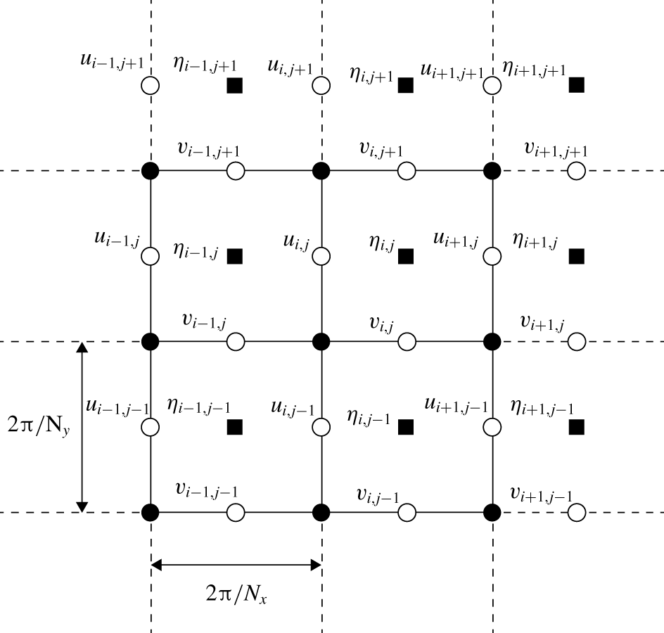
 $f=g=1$. The Arakawa C-gird is adopted (Haidvogel & Beckmann Reference Haidvogel and Beckmann1999), in which the variables
 $u,v,\unicode[STIX]{x1D702}$ are evaluated at different grid points (figure 1). The total number of grid points in the model is
 $3\times N_{x}\times N_{y}=3\times 128\times 128$. The time integration is performed using the leapfrog scheme.
The staggered grids used in the numerical model. Because variables  $u,v,\unicode[STIX]{x1D702}$ are evaluated at different points, the phase shift for each wavenumber component has to be taken into account, as described in (3.17).

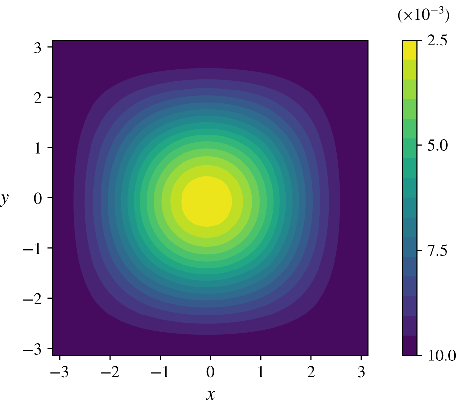
Water depth  $H(x,y)$ in the numerical model. The bright area in the centre of the domain corresponds to the shallow region.

The bottom topography is
 $$\begin{eqnarray}H(x,y)=1.0\times 10^{-2}-\frac{7.5\times 10^{-3}(1+\cos x)(1+\cos y)}{4},\end{eqnarray}$$
as depicted in figure 2. A localised wave packet,
 $$\begin{eqnarray}\unicode[STIX]{x1D702}=1.0\times 10^{-5}\exp \left(-\frac{x^{2}+(y+\unicode[STIX]{x03C0}/2)^{2}}{2(\unicode[STIX]{x03C0}/6)^{2}}\right)\sin (8.0x),\quad u=0,v=0,\end{eqnarray}$$
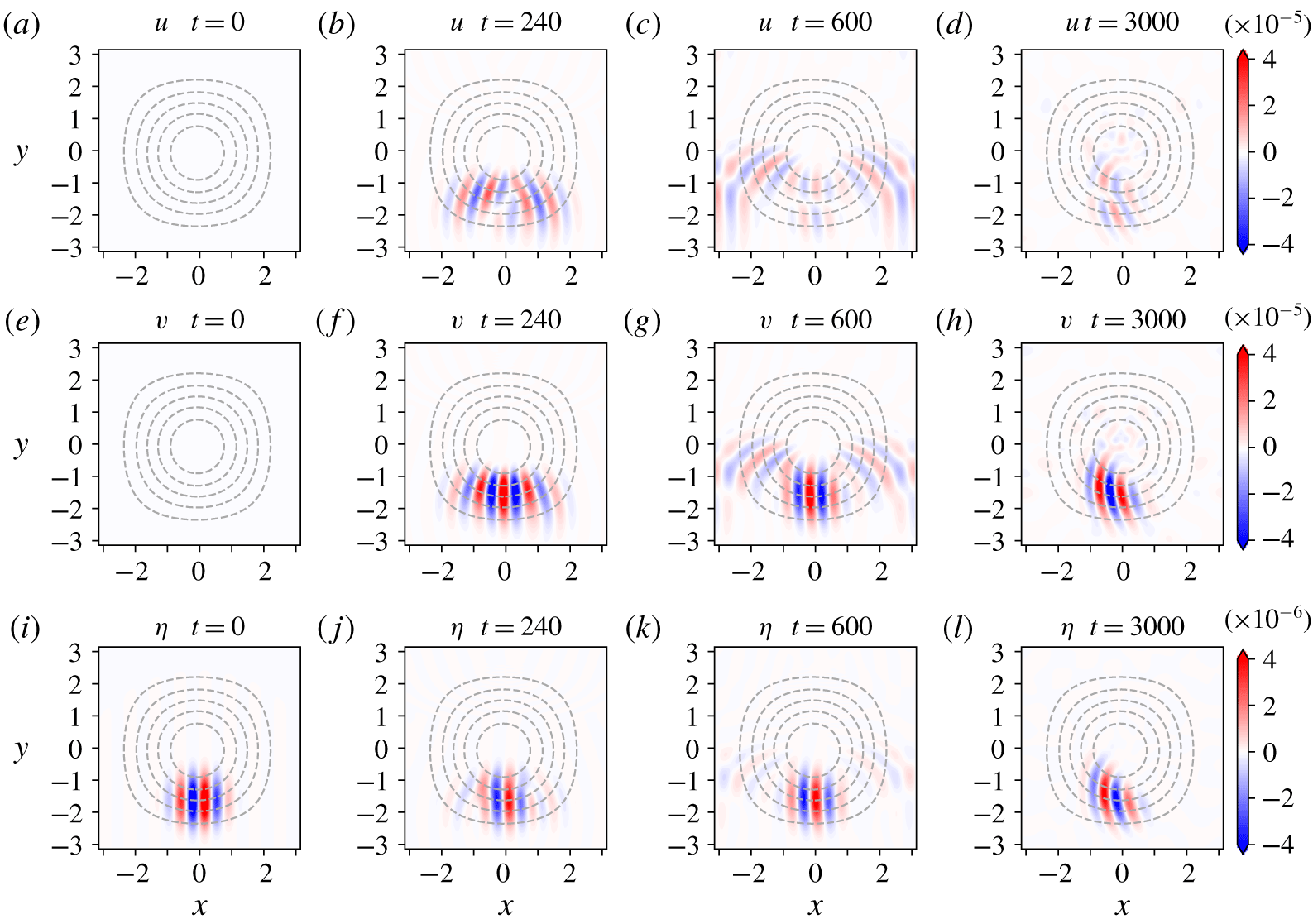
is arranged as the initial state and then allowed to propagate freely in the domain. Figure 3 shows a time series of the flow field. As the basic geostrophic adjustment, a pair of IGWs are immediately radiated away in opposite directions from the initial packet zone, whereas part of the flow field is left behind, almost retaining the geostrophic balance. This quasi-geostrophic flow pattern will also propagate leftward as an RW. This result suggests that the initial flow field was composed of a superposition of two distinguished wave modes, the IGW and the RW. The main objective is to decompose these modes and analyse their properties independently.
Results of the numerical simulation. (a–d) Zonal velocity  $u$, (e–h) meridional velocity
 $v$ and (i–l) surface elevation
 $\unicode[STIX]{x1D702}$ are shown at
 $t=0,240,600,3000$. Dashed curves are contours of the reference depth
 $H(x,y)$. The rapidly propagating inertia–gravity wave and the slowly propagating Rossby wave are overlapping.

To achieve this goal, we need to prepare a discrete form of the pseudo-differential operator (2.8). In general, formulae for operations among symbols based on star products can be constructed up to the infinite order of  $\unicode[STIX]{x1D707}$. However, for practical purposes we must truncate a perturbation series at a finite order. The first-order truncation is the most convenient choice because it enables the application of fast Fourier transform (FFT) in the calculation of the pseudo-differential operator.
First, by taking the ‘central difference’ with respect to  $\boldsymbol{x}$ and
 $\boldsymbol{x}^{\prime }$, we separate (2.8) approximately into two parts as
 $$\begin{eqnarray}\unicode[STIX]{x1D65B}(\hat{\boldsymbol{x}},\hat{\boldsymbol{p}})\unicode[STIX]{x1D753}=\frac{\unicode[STIX]{x1D743}(\boldsymbol{x})+\unicode[STIX]{x1D73B}(\boldsymbol{x})}{2}+O(\unicode[STIX]{x1D707}^{2}),\end{eqnarray}$$
where
 $$\begin{eqnarray}\displaystyle & \displaystyle \unicode[STIX]{x1D743}(\boldsymbol{x})\equiv \frac{1}{(2\unicode[STIX]{x03C0}\unicode[STIX]{x1D707})^{d}}\iint \unicode[STIX]{x1D65B}(\boldsymbol{x},\boldsymbol{p})\unicode[STIX]{x1D753}(\boldsymbol{x}^{\prime })\text{e}^{\text{i}\boldsymbol{p}\boldsymbol{\cdot }(\boldsymbol{x}-\boldsymbol{x}^{\prime })/\unicode[STIX]{x1D707}}\,\text{d}\boldsymbol{p}\,\text{d}\boldsymbol{x}^{\prime }, & \displaystyle\end{eqnarray}$$
 $$\begin{eqnarray}\displaystyle & \displaystyle \unicode[STIX]{x1D73B}(\boldsymbol{x})\equiv \frac{1}{(2\unicode[STIX]{x03C0}\unicode[STIX]{x1D707})^{d}}\iint \unicode[STIX]{x1D65B}(\boldsymbol{x}^{\prime },\boldsymbol{p})\unicode[STIX]{x1D753}(\boldsymbol{x}^{\prime })\text{e}^{\text{i}\boldsymbol{p}\boldsymbol{\cdot }(\boldsymbol{x}-\boldsymbol{x}^{\prime })/\unicode[STIX]{x1D707}}\,\text{d}\boldsymbol{p}\,\text{d}\boldsymbol{x}^{\prime }. & \displaystyle\end{eqnarray}$$
 $$\begin{eqnarray}\displaystyle & \displaystyle \unicode[STIX]{x1D743}_{ij}=\mathop{\sum }_{k=-N_{x}/2+1}^{N_{x}/2}\mathop{\sum }_{l=-N_{y}/2+1}^{N_{y}/2}\unicode[STIX]{x1D65B}_{ijkl}\tilde{\unicode[STIX]{x1D753}}_{kl}\text{e}^{2\unicode[STIX]{x03C0}\text{i}(ki/N_{x}+lj/N_{y})}, & \displaystyle\end{eqnarray}$$
 $$\begin{eqnarray}\displaystyle & \displaystyle \tilde{\unicode[STIX]{x1D753}}_{kl}=\frac{1}{N_{x}N_{y}}\mathop{\sum }_{i=-N_{x}/2+1}^{N_{x}/2}\mathop{\sum }_{j=-N_{y}/2+1}^{N_{y}/2}\unicode[STIX]{x1D753}_{ij}\text{e}^{-2\unicode[STIX]{x03C0}\text{i}(ki/N_{x}+lj/N_{y})}, & \displaystyle\end{eqnarray}$$
 $$\begin{eqnarray}\displaystyle & \displaystyle \unicode[STIX]{x1D73B}_{ij}=\mathop{\sum }_{k=-N_{x}/2+1}^{N_{x}/2}\mathop{\sum }_{l=-N_{y}/2+1}^{N_{y}/2}\tilde{\unicode[STIX]{x1D73B}}_{kl}\text{e}^{2\unicode[STIX]{x03C0}\text{i}(ki/N_{x}+lj/N_{y})}, & \displaystyle\end{eqnarray}$$
 $$\begin{eqnarray}\displaystyle & \displaystyle \tilde{\unicode[STIX]{x1D73B}}_{kl}=\frac{1}{N_{x}N_{y}}\mathop{\sum }_{i=-N_{x}/2+1}^{N_{x}/2}\mathop{\sum }_{j=-N_{y}/2+1}^{N_{y}/2}\unicode[STIX]{x1D65B}_{ijkl}\unicode[STIX]{x1D753}_{ij}\text{e}^{-2\unicode[STIX]{x03C0}\text{i}(ki/N_{x}+lj/N_{y})}. & \displaystyle\end{eqnarray}$$
 $u,v,\unicode[STIX]{x1D702}$ are evaluated at different points (figure 1). Therefore, a phase shift for each wavenumber component is taken into account; i.e. the discrete Fourier transform for each variable of
 $\unicode[STIX]{x1D74D}=(\sqrt{H/2}u,\sqrt{H/2}v,\sqrt{g/2}\unicode[STIX]{x1D702})^{\text{T}}$ is redefined as
 $$\begin{eqnarray}\displaystyle & \displaystyle \tilde{\unicode[STIX]{x1D713}}_{1kl}=\frac{1}{N_{x}N_{y}}\mathop{\sum }_{i=-N_{x}/2+1}^{N_{x}/2}\mathop{\sum }_{j=-N_{y}/2+1}^{N_{y}/2}\unicode[STIX]{x1D713}_{1ij}\text{e}^{-2\unicode[STIX]{x03C0}\text{i}(k(i-1/2)/N_{x}+lj/N_{y})}, & \displaystyle\end{eqnarray}$$
 $$\begin{eqnarray}\displaystyle & \displaystyle \tilde{\unicode[STIX]{x1D713}}_{2kl}=\frac{1}{N_{x}N_{y}}\mathop{\sum }_{i=-N_{x}/2+1}^{N_{x}/2}\mathop{\sum }_{j=-N_{y}/2+1}^{N_{y}/2}\unicode[STIX]{x1D713}_{2ij}\text{e}^{-2\unicode[STIX]{x03C0}\text{i}(ki/N_{x}+l(j-1/2)/N_{y})}, & \displaystyle\end{eqnarray}$$
 $$\begin{eqnarray}\displaystyle & \displaystyle \tilde{\unicode[STIX]{x1D713}}_{3kl}=\frac{1}{N_{x}N_{y}}\mathop{\sum }_{i=-N_{x}/2+1}^{N_{x}/2}\mathop{\sum }_{j=-N_{y}/2+1}^{N_{y}/2}\unicode[STIX]{x1D713}_{3ij}\text{e}^{-2\unicode[STIX]{x03C0}\text{i}(ki/N_{x}+lj/N_{y})}, & \displaystyle\end{eqnarray}$$
 $\unicode[STIX]{x1D74D}^{\prime }=(\unicode[STIX]{x1D713}_{g},\unicode[STIX]{x1D713}_{g}^{\dagger },\unicode[STIX]{x1D713}_{r})^{\text{T}}\equiv \unicode[STIX]{x1D66A}(\hat{\boldsymbol{x}},\hat{\boldsymbol{p}})\unicode[STIX]{x1D74D}$, to obtain the complex signals of IGWs and RWs, respectively. (Although (3.14) involves
 $O(\unicode[STIX]{x1D707})$ terms, because the symbol of the unitary operator
 $\unicode[STIX]{x1D66A}$ is prepared only in the
 $O(1)$ term, the result obtained is of leading-order accuracy. It is noted that the first-order correction of
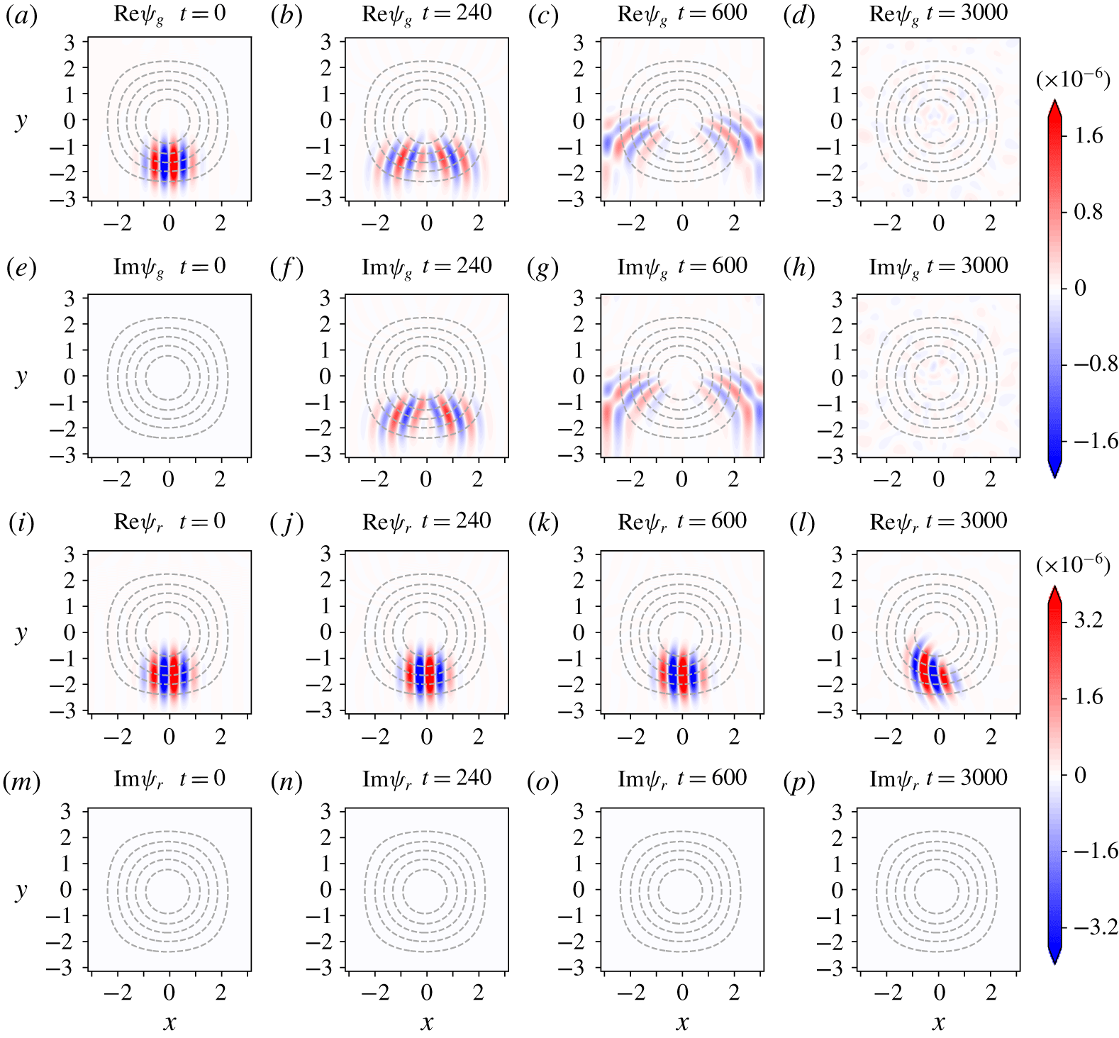
 $\unicode[STIX]{x1D66A}$ is too complicated to be written down explicitly, but its computation could be done by separately preparing the symbol matrices that composes (2.22) and combining them.) Figure 4 shows the real and imaginary parts of the complex signals
 $\unicode[STIX]{x1D713}_{g}$ and
 $\unicode[STIX]{x1D713}_{r}$. The two wave modes are successfully decomposed by this method.
Complex signals for the inertia–gravity wave and the Rossby wave, denoted as  $\unicode[STIX]{x1D713}_{g}$ and
 $\unicode[STIX]{x1D713}_{r}$, respectively. (a–d) Real parts of
 $\unicode[STIX]{x1D713}_{g}$, (e–h) imaginary parts of
 $\unicode[STIX]{x1D713}_{g}$, (i–l) real parts of
 $\unicode[STIX]{x1D713}_{r}$ and (m–p) imaginary parts of
 $\unicode[STIX]{x1D713}_{r}$ are shown at
 $t=0,240,600,3000$. Note that the imaginary parts of
 $\unicode[STIX]{x1D713}_{r}$ vanish for reasons that are explained in the text.

Next, we discretise the Wigner distribution function,  $w(\boldsymbol{x},\boldsymbol{p})$ as defined in (2.33). In this study, we adopt the discretised Wigner distribution function that corresponds to a discretised complex signal
 $\unicode[STIX]{x1D713}_{ij}$ as
 $$\begin{eqnarray}w_{ijkl}=\frac{4}{N_{x}N_{y}}\mathop{\sum }_{i^{\prime }=-N_{x}/2+1}^{N_{x}/2}\mathop{\sum }_{j^{\prime }=-N_{y}/2+1}^{N_{y}/2}\unicode[STIX]{x1D713}_{i+i^{\prime }j+j^{\prime }}\unicode[STIX]{x1D713}_{i-i^{\prime }j-j^{\prime }}^{\dagger }\text{e}^{-4\unicode[STIX]{x03C0}\text{i}(ki^{\prime }/N_{x}+lj^{\prime }/N_{y})},\end{eqnarray}$$
where indices of  $\unicode[STIX]{x1D713},\unicode[STIX]{x1D713}^{\dagger }$ are extended outside the domain taking advantage of the periodic boundary conditions. Expression (3.18) satisfies the total energy condition,
 $$\begin{eqnarray}\mathop{\sum }_{i=-N_{x}/2+1}^{N_{x}/2}\mathop{\sum }_{j=-N_{y}/2+1}^{N_{y}/2}|\unicode[STIX]{x1D713}_{ij}|^{2}=\mathop{\sum }_{i=-N_{x}/2+1}^{N_{x}/2}\mathop{\sum }_{j=-N_{y}/2+1}^{N_{y}/2}\mathop{\sum }_{k=-N_{x}/4+1}^{N_{x}/4}\mathop{\sum }_{l=-N_{y}/4+1}^{N_{y}/4}w_{ijkl}.\end{eqnarray}$$
In this definition, the maximum wavenumber of the Wigner distribution function becomes half the Nyquist wavenumber. To avoid this inconvenience, other definitions for the discrete Wigner distribution function have been suggested (Chassande-Mottin & Pai Reference Chassande-Mottin and Pai2005), although these are not discussed in detail here.
Projecting the transport equation (2.38) onto physical space, we define the energy density,  $E(\boldsymbol{x})=(2\unicode[STIX]{x03C0}\unicode[STIX]{x1D707})^{-2}\int w\,\text{d}\boldsymbol{p}$, and its flux,
 $\boldsymbol{F}(\boldsymbol{x})=(2\unicode[STIX]{x03C0}\unicode[STIX]{x1D707})^{-2}\int \boldsymbol{c}_{x}w\,\text{d}\boldsymbol{p}$. Their discretised forms are
 $$\begin{eqnarray}\displaystyle & \displaystyle E_{ij}=\mathop{\sum }_{k=-N_{x}/4+1}^{N_{x}/4}\mathop{\sum }_{l=-N_{y}/4+1}^{N_{y}/4}w_{ijkl}, & \displaystyle\end{eqnarray}$$
 $$\begin{eqnarray}\displaystyle & \displaystyle \boldsymbol{F}_{ij}=\mathop{\sum }_{k=-N_{x}/4+1}^{N_{x}/4}\mathop{\sum }_{l=-N_{y}/4+1}^{N_{y}/4}\boldsymbol{c}_{ijkl}w_{ijkl}, & \displaystyle\end{eqnarray}$$
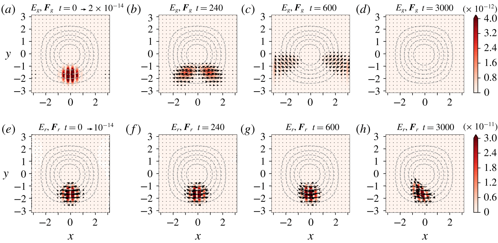
 $\boldsymbol{c}_{ijkl}$ is the group velocity of each wave specified in (3.11). Energy density and flux are calculated using these expressions and depicted in figure 5, which exhibits the wave energy propagation associated with each mode. However, the energy density and flux of the RW oscillate with the half-length of its wave packet, reflecting the phase variation in the signal. Such a feature is not seen in the case of IGWs except for the initial time (figures 4a,e and 5a) when the two-way propagating wave packets are overlapping. Historically, the phase dependence of the flux of RWs has been recognised as a nuisance by atmospheric scientists and overcome such as by Plumb (Reference Plumb1985) and Takaya & Nakamura (Reference Takaya and Nakamura2001). While these studies heuristically derived phase-independent representations of the pseudo-momentum flux associated with RWs, here we offer a more systematic consideration to solve this problem.
Energy density and (vector) fluxes for (a–d) the inertia–gravity wave and (e–h) the Rossby wave at  $t=0,240,600,3000$. A spatially oscillating structure arises in the case of the Rossby wave.

What causes the differences between IGWs and RWs? Why do only RWs exhibit an oscillating energy density in this analysis? A simple answer can be found when focusing on their dispersion relations. As (3.9c) shows, the dispersion relation of RWs is an odd function with respect to wavenumber; i.e.  $\unicode[STIX]{x1D714}(\boldsymbol{x},\boldsymbol{p})=-\unicode[STIX]{x1D714}(\boldsymbol{x},-\boldsymbol{p})$ holds. In this case, a solution of
 $$\begin{eqnarray}\text{i}\frac{\unicode[STIX]{x2202}\unicode[STIX]{x1D713}}{\unicode[STIX]{x2202}t}=\unicode[STIX]{x1D714}(\hat{\boldsymbol{x}},\hat{\boldsymbol{p}})\unicode[STIX]{x1D713}\end{eqnarray}$$
is also a solution of
 $$\begin{eqnarray}\text{i}\frac{\unicode[STIX]{x2202}\unicode[STIX]{x1D713}^{\dagger }}{\unicode[STIX]{x2202}t}=\unicode[STIX]{x1D714}(\hat{\boldsymbol{x}},\hat{\boldsymbol{p}})\unicode[STIX]{x1D713}^{\dagger }.\end{eqnarray}$$
Therefore, we can assume a solution satisfying  $\unicode[STIX]{x1D713}=\unicode[STIX]{x1D713}^{\dagger }$; i.e.
 $\unicode[STIX]{x1D713}$ can be a real function. In figure 4, it is indeed seen that the complex signal of the RW,
 $\unicode[STIX]{x1D713}_{r}$, possesses only the real part, whereas that of the IGWs,
 $\unicode[STIX]{x1D713}_{g}$, has both the real and imaginary parts, which is a consequence of the dispersion relation of IGWs not being an odd function. As inferred from the contrasting expressions,
 $|\text{cos}\,x|^{2}=(1+\cos 2x)/2$ and
 $|\text{e}^{\text{i}x}|^{2}=1$, energy and flux of the real RW signals always oscillate but those of the complex IGW signals do not.
This oscillatory structure of the RW can be removed by introducing a filtering technique. Using the Heaviside function  $V(x)$ that satisfies
 $V(x)=0$ for
 $x<0$ and
 $V(x)=1$ for
 $x>0$, let us define a symbol
 $v_{\unicode[STIX]{x1D714}}(\boldsymbol{x},\boldsymbol{p})=V(\unicode[STIX]{x1D714}(\boldsymbol{x},\boldsymbol{p}))$. Then, the operator
 $v_{\unicode[STIX]{x1D714}}(\hat{\boldsymbol{x}},\hat{\boldsymbol{p}})$ acts as a filter that transmits only the positive frequency components. As is obvious from its definition,
 $v_{\unicode[STIX]{x1D714}}(\hat{\boldsymbol{x}},\hat{\boldsymbol{p}})$ commutes with
 $\unicode[STIX]{x1D714}(\hat{\boldsymbol{x}},\hat{\boldsymbol{p}})$;
 $v_{\unicode[STIX]{x1D714}}(\hat{\boldsymbol{x}},\hat{\boldsymbol{p}})\unicode[STIX]{x1D714}(\hat{\boldsymbol{x}},\hat{\boldsymbol{p}})=\unicode[STIX]{x1D714}(\hat{\boldsymbol{x}},\hat{\boldsymbol{p}})v_{\unicode[STIX]{x1D714}}(\hat{\boldsymbol{x}},\hat{\boldsymbol{p}})$. From this property, the operation of
 $v_{\unicode[STIX]{x1D714}}(\hat{\boldsymbol{x}},\hat{\boldsymbol{p}})$ on (3.21) yields
 $$\begin{eqnarray}\text{i}\frac{\unicode[STIX]{x2202}}{\unicode[STIX]{x2202}t}(v_{\unicode[STIX]{x1D714}}(\hat{\boldsymbol{x}},\hat{\boldsymbol{p}})\unicode[STIX]{x1D713})=\unicode[STIX]{x1D714}(\hat{\boldsymbol{x}},\hat{\boldsymbol{p}})(v_{\unicode[STIX]{x1D714}}(\hat{\boldsymbol{x}},\hat{\boldsymbol{p}})\unicode[STIX]{x1D713}),\end{eqnarray}$$
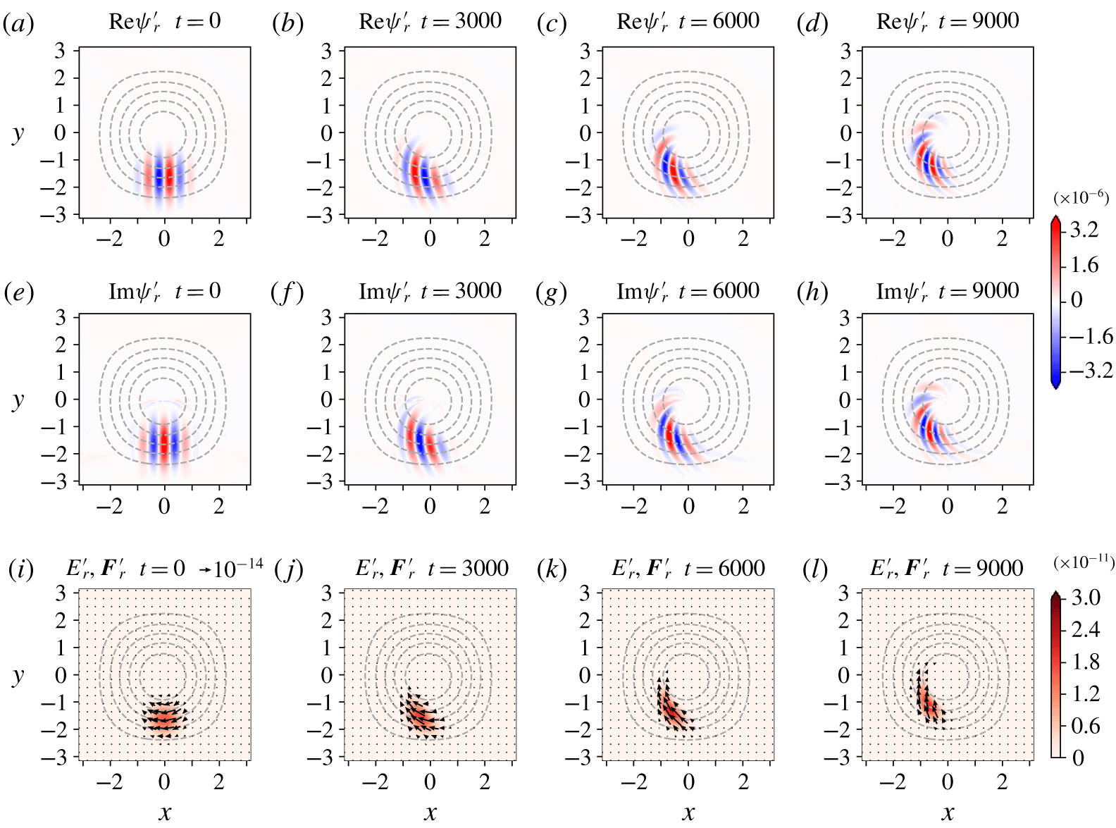
which means that  $v_{\unicode[STIX]{x1D714}}(\hat{\boldsymbol{x}},\hat{\boldsymbol{p}})\unicode[STIX]{x1D713}$ is also a solution of the original equation (3.21) and, moreover, it possesses both the real and imaginary parts. Figure 6 shows the filtered RW signal
 $\unicode[STIX]{x1D713}_{r}^{\prime }\equiv v_{\unicode[STIX]{x1D714}}(\hat{\boldsymbol{x}},\hat{\boldsymbol{p}})\unicode[STIX]{x1D713}_{r}$ and its associated energy density and flux. Both the real and imaginary parts of
 $\unicode[STIX]{x1D713}_{r}^{\prime }$ appear and the oscillatory structure of the energy density and flux is eliminated. It is noted that this filtering method resembles that in Sato, Kinoshita & Okamoto (Reference Sato, Kinoshita and Okamoto2013). In Sato et al. (Reference Sato, Kinoshita and Okamoto2013), the filtering function is defined in zonal wavenumber space by assuming a zonally symmetric background field, whereas the method presented here is a more general approach because it adaptively takes account of the local dispersion relation that varies from place to place.
(a–d) Real parts and (e–h) imaginary parts of the filtered complex signal of the Rossby wave,  $\unicode[STIX]{x1D713}_{r}^{\prime }=v_{\unicode[STIX]{x1D714}}(\hat{\boldsymbol{x}},\hat{\boldsymbol{p}})\unicode[STIX]{x1D713}_{r}$, and (i–l) its associated energy density
 $E_{r}^{\prime }$ and flux
 $\boldsymbol{F}_{r}^{\prime }$ at
 $t=0,3000,6000,9000$. Note that times
 $t$ are different from those in the previous figures.

4 Discussion and conclusions
This paper develops a general theoretical framework for wave decomposition in a slowly varying medium. The Wigner transform, which links an operator to a function, and its associated pseudo-differential operator provide a good perspective on this issue. Based on the asymptotic expansion of pseudo-differential operators, we construct a procedure to decompose a linearised fluid system into mutually independent wave signals, each of which is governed by a single wave equation  $\text{i}\unicode[STIX]{x2202}\unicode[STIX]{x1D713}/\unicode[STIX]{x2202}t=\unicode[STIX]{x1D714}(\hat{\boldsymbol{x}},\hat{\boldsymbol{p}})\unicode[STIX]{x1D713}$. During this, the polarisation relations
 $\unicode[STIX]{x1D66A}(\boldsymbol{x},\boldsymbol{p})$ and the dispersion relations
 $\unicode[STIX]{x1D74E}(\boldsymbol{x},\boldsymbol{p})$ are systematically derived up to any order of accuracy. According to the formulation in § 2, this decomposition is possible if either of the following two conditions is satisfied:
(i) The leading-order dispersion relations are non-degenerate.
(ii) The leading-order dispersion relations of degenerate modes are identically
 $0$ and resolved in the first order.

Some types of waves, such as electromagnetic waves or elastic waves, do not belong to these classes; degenerate polarised modes cannot be decomposed quasi-locally. The classical transport theory, therefore, takes account of the correlation of degenerate modes (Ryzhik et al. Reference Ryzhik, Papanicolaou and Keller1996). However, typical waves in the ocean and atmosphere, such as sound waves, IGWs and RWs, are decomposable. It is particularly noteworthy that barotropic and baroclinic RWs in a stratified fluid are degenerate as the zero-frequency mode in the leading-order description, but decomposed in the  $O(\unicode[STIX]{x1D707})$ terms.
The main content of the paper is the presentation of a practical method to diagnose flux of energy (or other conserved quantities) possessed by each wave signal, making use of the transport theory applied to model output data. The flux derived in the current approach satisfies the group velocity property  $\boldsymbol{F}\sim E\boldsymbol{c}_{g}$ in the plane-wave limit, where
 $\boldsymbol{F}$,
 $E$ and
 $\boldsymbol{c}_{g}$ are energy flux, energy density and group velocity, respectively. A filtering method is also introduced, which ensures the phase independence of energy density and its flux even for RWs. To the author’s best knowledge, this study is the first to separately analyse the fluxes associated with IGWs and RWs in one model with a solid theoretical basis. It is noted that, if we compose the Wigner distribution function numerically,
 $N_{x}^{2}\times N_{y}^{2}$ (
 $\times$ time steps) variables have to be stored in the two-dimensional case. However, for the practical purpose of visualising the energy flux in physical or wavenumber space, what we need is the energy density and flux projected onto each space, such as
 $E_{ij}$ and
 $\boldsymbol{F}_{ij}$ in (3.20). They can be calculated at each grid point,
 $(i,j)$, separately. Therefore, we actually do not need a large computer memory.
Here, we discuss the difference between the present method and some relevant works. First, the study of wave–vortex decomposition has a long history. Most of the works have focused on the effect from nonlinear couplings (e.g. Machenhauer Reference Machenhauer1977; Warn et al. Reference Warn, Bokhove, Shepherd and Vallis1995; Vanneste Reference Vanneste2013; Yasuda, Sato & Sugimoto Reference Yasuda, Sato and Sugimoto2015; Chouksey, Eden & Brüggemann Reference Chouksey, Eden and Brüggemann2018), where the vortex component is specifically named the ‘balanced’ mode. Asymptotic expansion with respect to the Rossby or Froude number has revealed how nonlinearity modifies the balanced mode. This study, on the other hand, considers the corrections of the linear polarisation and dispersion relations of every mode due to inhomogeneity based on asymptotic expansion with respect to the WKBJ parameter. Extending the current study to the cases of finite-amplitude waves will be an important future work. Second, one may find other types of linear wave–vortex decomposition using a numerical eigenvalue analysis. For example, Žagar et al. (Reference Žagar, Kasahara, Terasaki, Tribbia and Tanaka2015) offered numerical decomposition of IGWs and RWs with the use of eigenfunction expansion on a sphere. This type of method is effective to analyse waves with spatial scales comparable with the size of a closed domain. The current method, on the other hand, is inherently applicable to local wave packets existing in an infinite domain. Third, the classical transport theory has incorporated effect from inhomogeneity of a medium as scattering terms (Powell & Vanneste Reference Powell and Vanneste2005). The present method can also include the scattering effect into the formulation if we take account of rapid variations in the coefficient parameters. It is expected that a future study will also evaluate the scattering terms using model output data in the presence of, e.g. small-scale random topography.
Finally, the location of this study in a wide class of ray theory is considered. In the conventional ray-tracing method, propagation of wave action density is described by the equations  $\unicode[STIX]{x2202}A/\unicode[STIX]{x2202}t+\unicode[STIX]{x1D735}_{x}\boldsymbol{\cdot }(\dot{\boldsymbol{x}}A)=0,~\dot{\boldsymbol{x}}=\unicode[STIX]{x1D735}_{k}\unicode[STIX]{x1D714}$, and
 $\dot{\boldsymbol{k}}=-\unicode[STIX]{x1D735}_{x}\unicode[STIX]{x1D714}$, where the dispersion relation
 $\unicode[STIX]{x1D714}(\boldsymbol{x},\boldsymbol{k})$ should be preliminarily given (Lighthill Reference Lighthill1978). The current study offers a formulation which is valid one order higher than the conventional studies; the dispersion relation involves
 $O(\unicode[STIX]{x1D707})$ terms which is meaningful in the transport equation (2.38) with
 $O(\unicode[STIX]{x1D707}^{2})$ accuracy, whereas the classical ray tracing involves only the leading-order terms in the dispersion relation, which makes the action conservation equation of
 $O(\unicode[STIX]{x1D707})$ (Whitham Reference Whitham1970; Vanneste & Shepherd Reference Vanneste and Shepherd1999). This study rationalises that the shift of dispersion relation caused by the gradients in parameters can become meaningful in ray tracing, which is the case for RWs or even for IGWs in a frontal area, as has been pointed out in § 1.
Although this study applies the developed techniques only to the energy analysis of IGWs and RWs in a simple shallow water model, their pseudo-momentum and its associated residual volume transport will also be accessible in the same manner by computing the displacements of fluid parcels based on the velocity and frequency data and applying them to the generalised Lagrangian mean formulation (Bühler Reference Bühler2014). Application to a stratified fluid with background mean flow is another important step. The methodology can also be extended to forced–dissipative systems, as noted in appendix C, as well as including scattering effect. The new wave decomposition method introduced here will become useful as a data diagnostic technique for various situations in atmospheric and oceanic research.
Acknowledgements
The author expresses his gratitude to H. Aiki, N. Zhao and two anonymous reviewers for their invaluable comments on the original manuscript. Fruitful discussions with S. Inagaki, Y. Kosuga and M. Sasaki are also gratefully acknowledged. This study was supported by JSPS KAKENHI grant number JP16H02226 and the Collaborative Research Program of Research Institute for Applied Mechanics, Kyushu University. The numerical model code of the shallow water equation was originally developed by C.-H. Kim and J.-H. Yoon.
Appendix A. Derivation of the star product
Looking back on the definition of the Wigner transform (2.8), one may first find the representation of the star product as
 $$\begin{eqnarray}\displaystyle & & \displaystyle \unicode[STIX]{x1D65B}(\boldsymbol{x},\boldsymbol{p})\star \unicode[STIX]{x1D65C}(\boldsymbol{x},\boldsymbol{p})\nonumber\\ \displaystyle & & \displaystyle \quad =\frac{1}{(\unicode[STIX]{x03C0}\unicode[STIX]{x1D707})^{2d}}\iiiint \unicode[STIX]{x1D65B}(\boldsymbol{x}+\boldsymbol{x}^{\prime },\boldsymbol{p}+\boldsymbol{p}^{\prime })\unicode[STIX]{x1D65C}(\boldsymbol{x}+\boldsymbol{x}^{\prime \prime },\boldsymbol{p}+\boldsymbol{p}^{\prime \prime })\text{e}^{2\text{i}(\boldsymbol{p}^{\prime \prime }\boldsymbol{\cdot }\boldsymbol{x}^{\prime }-\boldsymbol{p}^{\prime }\boldsymbol{\cdot }\boldsymbol{x}^{\prime \prime })/\unicode[STIX]{x1D707}}\,\text{d}\boldsymbol{x}^{\prime }\,\text{d}\boldsymbol{x}^{\prime \prime }\,\text{d}\boldsymbol{p}^{\prime }\,\text{d}\boldsymbol{p}^{\prime \prime }.\nonumber\\ \displaystyle & & \displaystyle\end{eqnarray}$$
It may be worth noting that (A 1) exhibits the associative law of the star product;  $(\unicode[STIX]{x1D65B}\star \unicode[STIX]{x1D65C})\star \unicode[STIX]{x1D65D}=\unicode[STIX]{x1D65B}\star (\unicode[STIX]{x1D65C}\star \unicode[STIX]{x1D65D})$. Using the conventional formula
 $$\begin{eqnarray}\frac{1}{2\unicode[STIX]{x03C0}\unicode[STIX]{x1D707}}\iint x^{n}p^{m}\text{e}^{\text{i}px/\unicode[STIX]{x1D707}}\,\text{d}x\,\text{d}p=\left\{\begin{array}{@{}ll@{}}(\text{i}\unicode[STIX]{x1D707})^{n}n! & (n=m)\\ 0 & (n\neq m),\end{array}\right.\end{eqnarray}$$
which combined with Taylor expansion leads to
 $$\begin{eqnarray}\frac{1}{2\unicode[STIX]{x03C0}\unicode[STIX]{x1D707}}\iint f(x+x^{\prime },p+p^{\prime })\text{e}^{\text{i}p^{\prime }x^{\prime }/\unicode[STIX]{x1D707}}\,\text{d}x^{\prime }\,\text{d}p^{\prime }=\mathop{\sum }_{n=0}^{\infty }\frac{(\text{i}\unicode[STIX]{x1D707})^{n}}{n!}\frac{\unicode[STIX]{x2202}^{2n}f(x,p)}{\unicode[STIX]{x2202}_{x}^{n}\unicode[STIX]{x2202}_{p}^{n}},\end{eqnarray}$$
equation (A 1) can be expanded with respect to  $\unicode[STIX]{x1D707}$ to yield (2.10).
Appendix B. Accuracy of the dispersion relation
In § 2, we have shown that the dispersion relation  $\unicode[STIX]{x1D714}(\boldsymbol{x},\boldsymbol{p})$ is derived by diagonalising
 $\unicode[STIX]{x1D65D}(\boldsymbol{x},\boldsymbol{p})$ that specifies the time evolution of the system. The dispersion relation that is obtained generally involves infinite number of terms expanded in a power series with respect to
 $\unicode[STIX]{x1D707}$. A question then arises as to whether or not the higher-order components in
 $\unicode[STIX]{x1D714}$ are meaningful in view of the actual wave property. The traditional WKBJ analysis offers a clear answer to this question. Let us consider a single (pseudo-)differential equation
 $$\begin{eqnarray}\displaystyle \text{i}\frac{\unicode[STIX]{x2202}\unicode[STIX]{x1D713}}{\unicode[STIX]{x2202}t}=\unicode[STIX]{x1D714}(\hat{\boldsymbol{x}},\hat{\boldsymbol{p}})\unicode[STIX]{x1D713}, & & \displaystyle\end{eqnarray}$$
and seek its solution with a single frequency,  $\unicode[STIX]{x1D713}(\boldsymbol{x},t)=\tilde{\unicode[STIX]{x1D713}}(\boldsymbol{x})\text{e}^{-\text{i}\unicode[STIX]{x1D70E}t}$. Substitution of this in (B 1) yields
 $$\begin{eqnarray}(\unicode[STIX]{x1D70E}-\unicode[STIX]{x1D714}(\hat{\boldsymbol{x}},\hat{\boldsymbol{p}}))\tilde{\unicode[STIX]{x1D713}}(\boldsymbol{x})=0.\end{eqnarray}$$
Here we assume that the symbol  $\unicode[STIX]{x1D714}(\boldsymbol{x},\boldsymbol{p})$ is a real function and also that the frequency
 $\unicode[STIX]{x1D70E}$ is a real number. These are expanded with respect to
 $\unicode[STIX]{x1D707}$ as
 $$\begin{eqnarray}\displaystyle & \displaystyle \unicode[STIX]{x1D714}=\unicode[STIX]{x1D714}_{0}+\unicode[STIX]{x1D707}\unicode[STIX]{x1D714}_{1}+\cdots \,, & \displaystyle\end{eqnarray}$$
 $$\begin{eqnarray}\displaystyle & \displaystyle \unicode[STIX]{x1D70E}=\unicode[STIX]{x1D70E}_{0}+\unicode[STIX]{x1D707}\unicode[STIX]{x1D70E}_{1}+\cdots \,. & \displaystyle\end{eqnarray}$$
 $\unicode[STIX]{x1D707}$ as
 $$\begin{eqnarray}\displaystyle \tilde{\unicode[STIX]{x1D713}}(\boldsymbol{x}) & = & \displaystyle \exp \left(\frac{1}{\unicode[STIX]{x1D707}}\unicode[STIX]{x1D719}(\boldsymbol{x})\right)\nonumber\\ \displaystyle & = & \displaystyle \exp \left\{\frac{1}{\unicode[STIX]{x1D707}}(\text{i}\unicode[STIX]{x1D719}_{0}(\boldsymbol{x})+\unicode[STIX]{x1D707}(\unicode[STIX]{x1D719}_{1}^{r}(\boldsymbol{x})+\text{i}\unicode[STIX]{x1D719}_{1}^{i}(\boldsymbol{x}))+\cdots \,)\right\},\end{eqnarray}$$
where  $\unicode[STIX]{x1D719}_{0},\unicode[STIX]{x1D719}_{j}^{r},\unicode[STIX]{x1D719}_{j}^{i}$ are real functions. The imaginary part of the exponent,
 $$\begin{eqnarray}\unicode[STIX]{x1D6E9}(\boldsymbol{x})\equiv \unicode[STIX]{x1D719}_{0}+\unicode[STIX]{x1D707}\unicode[STIX]{x1D719}_{1}^{i}+\cdots \,,\end{eqnarray}$$
represents the phase of the wave solution and therefore its spatial derivative  $\unicode[STIX]{x1D735}_{x}\unicode[STIX]{x1D6E9}$ corresponds to the local wavenumber. Now we consider the power series expansion of
 $$\begin{eqnarray}\unicode[STIX]{x1D714}(\hat{\boldsymbol{x}},\hat{\boldsymbol{p}})\unicode[STIX]{x1D713}(\boldsymbol{x})=\frac{1}{(2\unicode[STIX]{x03C0}\unicode[STIX]{x1D707})^{d}}\iint \unicode[STIX]{x1D714}\left(\boldsymbol{x}+\frac{\boldsymbol{y}}{2},\boldsymbol{p}\right)\exp \left(\frac{-\text{i}\boldsymbol{p}\boldsymbol{\cdot }\boldsymbol{y}+\unicode[STIX]{x1D719}(\boldsymbol{x}+\boldsymbol{y})}{\unicode[STIX]{x1D707}}\right)\,\text{d}\boldsymbol{y}\,\text{d}\boldsymbol{p},\end{eqnarray}$$
where change of variable,  $\boldsymbol{y}=\boldsymbol{x}^{\prime }-\boldsymbol{x}$, is used in (2.8). We first derive
 $$\begin{eqnarray}\displaystyle & & \displaystyle \frac{1}{(2\unicode[STIX]{x03C0}\unicode[STIX]{x1D707})^{d}}\iint \unicode[STIX]{x1D714}\left(\boldsymbol{x}+\frac{\boldsymbol{y}}{2},\boldsymbol{p}\right)\exp \left(\frac{-\text{i}\boldsymbol{p}\boldsymbol{\cdot }\boldsymbol{y}}{\unicode[STIX]{x1D707}}\right)\,\text{d}\boldsymbol{y}\,\text{d}\boldsymbol{p}\nonumber\\ \displaystyle & & \displaystyle \quad =\frac{1}{(2\unicode[STIX]{x03C0}\unicode[STIX]{x1D707})^{d}}\iint \left(\unicode[STIX]{x1D714}(\boldsymbol{x},\boldsymbol{p})+\frac{1}{2}\unicode[STIX]{x1D735}_{x}\unicode[STIX]{x1D714}(\boldsymbol{x},\boldsymbol{p})\boldsymbol{\cdot }\boldsymbol{y}+O(|\boldsymbol{y}|^{2})\right)\exp \left(\frac{-\text{i}\boldsymbol{p}\boldsymbol{\cdot }\boldsymbol{y}}{\unicode[STIX]{x1D707}}\right)\,\text{d}\boldsymbol{y}\,\text{d}\boldsymbol{p}\nonumber\\ \displaystyle & & \displaystyle \quad =\frac{1}{(2\unicode[STIX]{x03C0}\unicode[STIX]{x1D707})^{d}}\iint \left(\unicode[STIX]{x1D714}(\boldsymbol{x},\boldsymbol{p})+\frac{\text{i}\unicode[STIX]{x1D707}}{2}\unicode[STIX]{x1D735}_{x}\unicode[STIX]{x1D714}(\boldsymbol{x},\boldsymbol{p})\boldsymbol{\cdot }\unicode[STIX]{x1D735}_{p}+O(\unicode[STIX]{x1D707}^{2})\right)\exp \left(\frac{-\text{i}\boldsymbol{p}\boldsymbol{\cdot }\boldsymbol{y}}{\unicode[STIX]{x1D707}}\right)\,\text{d}\boldsymbol{y}\,\text{d}\boldsymbol{p}\nonumber\\ \displaystyle & & \displaystyle \quad =\frac{1}{(2\unicode[STIX]{x03C0}\unicode[STIX]{x1D707})^{d}}\iint \left(\unicode[STIX]{x1D714}(\boldsymbol{x},\boldsymbol{p})-\frac{\text{i}\unicode[STIX]{x1D707}}{2}\unicode[STIX]{x1D735}_{x}\boldsymbol{\cdot }\unicode[STIX]{x1D735}_{p}\unicode[STIX]{x1D714}(\boldsymbol{x},\boldsymbol{p})+O(\unicode[STIX]{x1D707}^{2})\right)\nonumber\\ \displaystyle & & \displaystyle \qquad \times \,\exp \left(\frac{-\text{i}\boldsymbol{p}\boldsymbol{\cdot }\boldsymbol{y}}{\unicode[STIX]{x1D707}}\right)\,\text{d}\boldsymbol{y}\,\text{d}\boldsymbol{p}+(\text{surf})\nonumber\\ \displaystyle & & \displaystyle \quad =\frac{1}{(2\unicode[STIX]{x03C0}\unicode[STIX]{x1D707})^{d}}\iint \left(\unicode[STIX]{x1D714}_{0}(\boldsymbol{x},\boldsymbol{p})+\unicode[STIX]{x1D707}\left(\unicode[STIX]{x1D714}_{1}(\boldsymbol{x},\boldsymbol{p})-\frac{\text{i}}{2}\unicode[STIX]{x1D735}_{x}\boldsymbol{\cdot }\unicode[STIX]{x1D735}_{p}\unicode[STIX]{x1D714}_{0}(\boldsymbol{x},\boldsymbol{p})\right)+O(\unicode[STIX]{x1D707}^{2})\right)\nonumber\\ \displaystyle & & \displaystyle \qquad \times \,\exp \left(\frac{-\text{i}\boldsymbol{p}\boldsymbol{\cdot }\boldsymbol{y}}{\unicode[STIX]{x1D707}}\right)\,\text{d}\boldsymbol{y}\,\text{d}\boldsymbol{p}+(\text{surf}).\end{eqnarray}$$
Here the (surf) terms represent the contribution from the integral surface  $|\boldsymbol{p}|=\infty$. By assuming that
 $\tilde{\unicode[STIX]{x1D713}}$ is sufficiently smooth, we may neglect these terms hereafter. Additionally using
 $$\begin{eqnarray}\unicode[STIX]{x1D719}(\boldsymbol{x}+\boldsymbol{y})=\unicode[STIX]{x1D719}(\boldsymbol{x})+\unicode[STIX]{x1D735}_{x}\unicode[STIX]{x1D719}(\boldsymbol{x})\boldsymbol{\cdot }\boldsymbol{y}+{\textstyle \frac{1}{2}}(\unicode[STIX]{x1D735}_{x}\otimes \unicode[STIX]{x1D735}_{x})\unicode[STIX]{x1D719}(\boldsymbol{x})\boldsymbol{\cdot }(\boldsymbol{y}\otimes \boldsymbol{y})+O(|\boldsymbol{y}|^{3}),\end{eqnarray}$$
where  $\otimes$ denotes the outer product, we derive from (B 2) the following expression:
 $$\begin{eqnarray}\displaystyle & & \displaystyle \unicode[STIX]{x1D70E}-\frac{1}{(2\unicode[STIX]{x03C0}\unicode[STIX]{x1D707})^{d}}\iint \left[\exp \left(\frac{-\text{i}(\boldsymbol{p}-\unicode[STIX]{x1D735}_{x}\unicode[STIX]{x1D719}_{0}(\boldsymbol{x}))\boldsymbol{\cdot }\boldsymbol{y}}{\unicode[STIX]{x1D707}}\right)\right.\nonumber\\ \displaystyle & & \displaystyle \quad \times \exp \left(-\text{i}\unicode[STIX]{x1D707}\unicode[STIX]{x1D735}_{x}\unicode[STIX]{x1D719}_{1}^{r}(\boldsymbol{x})\boldsymbol{\cdot }\unicode[STIX]{x1D735}_{p}+\unicode[STIX]{x1D707}\unicode[STIX]{x1D735}_{x}\unicode[STIX]{x1D719}_{1}^{i}(\boldsymbol{x})\boldsymbol{\cdot }\unicode[STIX]{x1D735}_{p}-\frac{\text{i}\unicode[STIX]{x1D707}}{2}(\unicode[STIX]{x1D735}_{x}\otimes \unicode[STIX]{x1D735}_{x})\unicode[STIX]{x1D719}_{0}(\boldsymbol{x})\boldsymbol{\cdot }(\unicode[STIX]{x1D735}_{p}\otimes \unicode[STIX]{x1D735}_{p})\right)\nonumber\\ \displaystyle & & \displaystyle \quad \times \left.\left(\unicode[STIX]{x1D714}_{0}(\boldsymbol{x},\boldsymbol{p})+\unicode[STIX]{x1D707}\left(\unicode[STIX]{x1D714}_{1}(\boldsymbol{x},\boldsymbol{p})-\frac{\text{i}}{2}\unicode[STIX]{x1D735}_{x}\boldsymbol{\cdot }\unicode[STIX]{x1D735}_{p}\unicode[STIX]{x1D714}_{0}(\boldsymbol{x},\boldsymbol{p})\right)\right)\right]\,\text{d}\boldsymbol{y}\,\text{d}\boldsymbol{p}=O(\unicode[STIX]{x1D707}^{2}),\end{eqnarray}$$
which, after performing an integration, becomes
 $$\begin{eqnarray}\displaystyle & & \displaystyle \unicode[STIX]{x1D70E}-\left[\exp \left(-\text{i}\unicode[STIX]{x1D707}\unicode[STIX]{x1D735}_{x}\unicode[STIX]{x1D719}_{1}^{r}(\boldsymbol{x})\boldsymbol{\cdot }\unicode[STIX]{x1D735}_{p}+\unicode[STIX]{x1D707}\unicode[STIX]{x1D735}_{x}\unicode[STIX]{x1D719}_{1}^{i}(\boldsymbol{x})\boldsymbol{\cdot }\unicode[STIX]{x1D735}_{p}-\frac{\text{i}\unicode[STIX]{x1D707}}{2}(\unicode[STIX]{x1D735}_{x}\otimes \unicode[STIX]{x1D735}_{x})\unicode[STIX]{x1D719}_{0}(\boldsymbol{x})\boldsymbol{\cdot }(\unicode[STIX]{x1D735}_{p}\otimes \unicode[STIX]{x1D735}_{p})\right)\right.\nonumber\\ \displaystyle & & \displaystyle \quad \times \left.\left(\unicode[STIX]{x1D714}_{0}(\boldsymbol{x},\boldsymbol{p})+\unicode[STIX]{x1D707}\left(\unicode[STIX]{x1D714}_{1}(\boldsymbol{x},\boldsymbol{p})-\frac{\text{i}}{2}\unicode[STIX]{x1D735}_{x}\boldsymbol{\cdot }\unicode[STIX]{x1D735}_{p}\unicode[STIX]{x1D714}_{0}(\boldsymbol{x},\boldsymbol{p})\right)\right)\right]_{\boldsymbol{p}=\unicode[STIX]{x1D735}_{x}\unicode[STIX]{x1D719}_{0}}=O(\unicode[STIX]{x1D707}^{2}).\end{eqnarray}$$
Further expanding the exponential function, we obtain the leading- and first-order terms as
 $$\begin{eqnarray}\unicode[STIX]{x1D70E}_{0}=\unicode[STIX]{x1D714}_{0}(\boldsymbol{x},\boldsymbol{p}),\end{eqnarray}$$
 $$\begin{eqnarray}\displaystyle \unicode[STIX]{x1D70E}_{1} & = & \displaystyle \unicode[STIX]{x1D714}_{1}(\boldsymbol{x},\boldsymbol{p})-\frac{\text{i}}{2}\unicode[STIX]{x1D735}_{x}\boldsymbol{\cdot }\unicode[STIX]{x1D735}_{p}\unicode[STIX]{x1D714}_{0}(\boldsymbol{x},\boldsymbol{p})-\text{i}\unicode[STIX]{x1D735}_{x}\unicode[STIX]{x1D719}_{1}^{r}(\boldsymbol{x})\boldsymbol{\cdot }\unicode[STIX]{x1D735}_{p}\unicode[STIX]{x1D714}_{0}(\boldsymbol{x},\boldsymbol{p})+\unicode[STIX]{x1D735}_{x}\unicode[STIX]{x1D719}_{1}^{i}(\boldsymbol{x})\boldsymbol{\cdot }\unicode[STIX]{x1D735}_{p}\unicode[STIX]{x1D714}_{0}(\boldsymbol{x},\boldsymbol{p})\nonumber\\ \displaystyle & & \displaystyle -\,\frac{\text{i}}{2}(\unicode[STIX]{x1D735}_{x}\otimes \unicode[STIX]{x1D735}_{x})\unicode[STIX]{x1D719}_{0}(\boldsymbol{x})\boldsymbol{\cdot }(\unicode[STIX]{x1D735}_{p}\otimes \unicode[STIX]{x1D735}_{p})\unicode[STIX]{x1D714}_{0}(\boldsymbol{x},\boldsymbol{p}),\end{eqnarray}$$
 $\boldsymbol{p}=\unicode[STIX]{x1D735}_{x}\unicode[STIX]{x1D719}_{0}(\boldsymbol{x})$. The real part of (B 11b) is
 $$\begin{eqnarray}\unicode[STIX]{x1D70E}_{1}=\unicode[STIX]{x1D714}_{1}(\boldsymbol{x},\boldsymbol{p})+\unicode[STIX]{x1D735}_{x}\unicode[STIX]{x1D719}_{1}^{i}\boldsymbol{\cdot }\unicode[STIX]{x1D735}_{p}\unicode[STIX]{x1D714}_{0}(\boldsymbol{x},\boldsymbol{p}),\end{eqnarray}$$
which combined with (B 11a) yields
 $$\begin{eqnarray}\unicode[STIX]{x1D70E}=\unicode[STIX]{x1D714}(\boldsymbol{x},\unicode[STIX]{x1D735}_{x}(\unicode[STIX]{x1D719}_{0}(\boldsymbol{x})+\unicode[STIX]{x1D707}\unicode[STIX]{x1D719}_{1}^{i}(\boldsymbol{x})))+O(\unicode[STIX]{x1D707}^{2}).\end{eqnarray}$$
From this expression, we understand that by redefining the local wavenumber as $\boldsymbol{p}=\unicode[STIX]{x1D735}_{x}\unicode[STIX]{x1D6E9}$, the dispersion relation
 $\unicode[STIX]{x1D70E}=\unicode[STIX]{x1D714}(\boldsymbol{x},\boldsymbol{p})$ is valid up to the first-order perturbation terms. Therefore, the symbol
 $\unicode[STIX]{x1D714}(\boldsymbol{x},\boldsymbol{p})$ derived by the present diagonalisation method yields a dispersion relation of at least first-order accuracy.
In addition, using the imaginary part of (B 11b) that is
 $$\begin{eqnarray}\displaystyle 0 & = & \displaystyle -{\textstyle \frac{1}{2}}\unicode[STIX]{x1D735}_{x}\boldsymbol{\cdot }\unicode[STIX]{x1D735}_{p}\unicode[STIX]{x1D714}_{0}(\boldsymbol{x},\boldsymbol{p})-\unicode[STIX]{x1D735}_{x}\unicode[STIX]{x1D719}_{1}^{r}(\boldsymbol{x})\boldsymbol{\cdot }\unicode[STIX]{x1D735}_{p}\unicode[STIX]{x1D714}_{0}(\boldsymbol{x},\boldsymbol{p})\nonumber\\ \displaystyle & & \displaystyle -\,{\textstyle \frac{1}{2}}(\unicode[STIX]{x1D735}_{x}\otimes \unicode[STIX]{x1D735}_{x})\unicode[STIX]{x1D719}_{0}(\boldsymbol{x})\boldsymbol{\cdot }(\unicode[STIX]{x1D735}_{p}\otimes \unicode[STIX]{x1D735}_{p})\unicode[STIX]{x1D714}_{0}(\boldsymbol{x},\boldsymbol{p}),\end{eqnarray}$$
and defining the squared wave amplitude  $E(\boldsymbol{x})\equiv |\tilde{\unicode[STIX]{x1D713}}|^{2}$, we can derive the leading-order expression of an elementary conservation law for a steady wave train,
 $$\begin{eqnarray}\unicode[STIX]{x1D735}_{x}\boldsymbol{\cdot }(\unicode[STIX]{x1D735}_{p}\unicode[STIX]{x1D714}(\boldsymbol{x},\boldsymbol{p}(\boldsymbol{x}))E(\boldsymbol{x}))=O(\unicode[STIX]{x1D707}).\end{eqnarray}$$
Appendix C. Forced–dissipative system
In a general non-conservative system, linear wave motions are governed by an equation in the form of
 $$\begin{eqnarray}\displaystyle \text{i}\frac{\unicode[STIX]{x2202}\unicode[STIX]{x1D74D}}{\unicode[STIX]{x2202}t}=\hat{\unicode[STIX]{x1D647}}\unicode[STIX]{x1D74D}+\unicode[STIX]{x1D738}, & & \displaystyle\end{eqnarray}$$
where the operator  $\hat{\unicode[STIX]{x1D647}}$ is not necessarily Hermitian and
 $\unicode[STIX]{x1D738}$ represents external forcing. Supposing that
 $\hat{\unicode[STIX]{x1D647}}$ can be diagonalised as
 $\hat{\unicode[STIX]{x1D648}}\hat{\unicode[STIX]{x1D647}}\hat{\unicode[STIX]{x1D648}}^{-1}=\hat{\unicode[STIX]{x1D734}}$, transforming the state vector into
 $\unicode[STIX]{x1D74D}^{\prime }=\hat{\unicode[STIX]{x1D648}}\unicode[STIX]{x1D74D}$, the equation for the Wigner distribution function of the
 $i$th mode,
 $w(\boldsymbol{x},\boldsymbol{p})=\int \unicode[STIX]{x1D713}_{i}^{\prime }(\boldsymbol{x}+\boldsymbol{x}^{\prime }/2){\unicode[STIX]{x1D713}_{i}^{\prime }}^{\dagger }(\boldsymbol{x}-\boldsymbol{x}^{\prime }/2)\text{e}^{-\text{i}\boldsymbol{p}\boldsymbol{\cdot }\boldsymbol{x}^{\prime }/\unicode[STIX]{x1D707}}\,\text{d}\boldsymbol{x}^{\prime }$, is derived,
 $$\begin{eqnarray}\text{i}\frac{\unicode[STIX]{x2202}w}{\unicode[STIX]{x2202}t}=\unicode[STIX]{x1D714}\star w-w\star \unicode[STIX]{x1D714}^{\dagger }+\text{i}s,\end{eqnarray}$$
where the source term  $\text{i}s$ originates from
 $\unicode[STIX]{x1D738}$. The dispersion relation
 $\unicode[STIX]{x1D714}(\boldsymbol{x},\boldsymbol{p})$ now has real and imaginary parts. Defining
 $\unicode[STIX]{x1D70E}=\text{Re}\unicode[STIX]{x1D714}$ and
 $\unicode[STIX]{x1D708}=-2\text{Im}\unicode[STIX]{x1D714}$, we may rewrite (C 2) as
 $$\begin{eqnarray}\frac{\unicode[STIX]{x2202}w}{\unicode[STIX]{x2202}t}+\unicode[STIX]{x1D707}\unicode[STIX]{x1D735}_{p}\unicode[STIX]{x1D70E}\boldsymbol{\cdot }\unicode[STIX]{x1D735}_{x}w-\unicode[STIX]{x1D707}\unicode[STIX]{x1D735}_{x}\unicode[STIX]{x1D70E}\boldsymbol{\cdot }\unicode[STIX]{x1D735}_{p}w=-\unicode[STIX]{x1D708}w+s+O(\unicode[STIX]{x1D707}^{2}).\end{eqnarray}$$
In a dissipative system, the function  $\unicode[STIX]{x1D708}(\boldsymbol{x},\boldsymbol{p})$ usually (but not necessarily) takes a positive value, representing the decay rate of wave energy. Equation (C 3) is also a kind of transport equation (1.2).