1. Introduction
Tangled magnetic fields are ubiquitous in astrophysical systems, expected to develop in stellar interiors, accretion discs, galaxies and clusters of galaxies (Zel'dovich, Ruzmaikin & Sokoloff Reference Zel'dovich, Ruzmaikin and Sokoloff1983). Their ubiquity results from the freezing of magnetic flux into fluid motions in ideal magnetohydrodynamics (MHD): initially straight field lines are quickly tangled by the random stretching motions of a turbulent flow, typically at spatial scales smaller than those associated with the global flow (see, e.g. Rincon Reference Rincon2019).
If such turbulence is driven sporadically and the subsequent relaxation is viscously dominated (as will be the case when the magnetic Prandtl number  $Pm=\nu /\eta \gg 1$), or if the system relaxes to some quasi-stable steady state, then there may be periods of time when a dynamical-strength magnetic field tangled at small scales threads relatively quiescent fluid. The large-scale dynamic properties of such a fluid may be highly relevant for questions about how energy is propagated, stored and dissipated in the astrophysical systems described above. Such considerations motivate an idealised plasma physics problem: how does a static fluid with a statistically homogeneous and isotropic Maxwell stress respond to an imposed large-scale impulse? It is this question that we aim to address in this paper, subject to some important simplifying assumptions.
We will treat the problem in the setting of non-resistive MHD, i.e. assuming perfect flux freezing, and thus the invariance of the magnetic-field topology. Physically, this means assuming that the small-scale magnetic tangle is itself at scales sufficiently large for magnetic dissipation to be negligible. In pursuit of maximal simplicity, we will also assume that the tangled magnetic field represents an equilibrium state. While this assumption may be unrealistic for MHD turbulence, the dynamics of the tangled equilibrium field are sufficiently complex to warrant investigation, and we anticipate that the lessons learned here will inform study of the more realistic, non-equilibrium case, which we shall report in a later publication.
The plan of this paper is as follows. In § 2, we formally motivate the problem from the equations of ideal MHD, and describe previous work that modelled the equilibrium Maxwell stress as ‘perfectly’ homogeneous and isotropic at all scales. Using this model, Moffatt (Reference Moffatt1986) argued that tangled fields should support waves whose restoring force is the isotropic elasticity afforded by the magnetic field – these ‘magnetoelastic’ waves are the isotropic analogue of Alfvén waves on a straight magnetic field. Later, magnetoelastic waves were rederived by Gruzinov & Diamond (Reference Gruzinov and Diamond1996) in the same approximation, and were suggested (in a somewhat modified form) by Schekochihin et al. (Reference Schekochihin, Cowley, Hammett, Maron and McWilliams2002) and Maron, Cowley & McWilliams (Reference Maron, Cowley and McWilliams2004) as a possible mechanism for the saturation of the turbulent MHD dynamo. Williams (Reference Williams2004) has speculated on the importance of magnetoelasticity in astrophysical systems in which the presence of magnetic fields is traditionally modelled by magnetic viscosity. More recently, Chen & Diamond (Reference Chen and Diamond2020) have developed a theory of potential vorticity mixing in the solar tachocline, accounting for the effect of a tangled magnetic-field elasticity using a similar model. Experimentally, elastic waves have been observed in viscoelastic flows of polymer solutions (Qin et al. Reference Qin, Salipante, Hudson and Arratia2019), which obey a system of equations closely related to MHD (Ogilvie & Proctor Reference Ogilvie and Proctor2003).
However, treating the field as perfectly homogeneous naturally precludes the possibility of the large-scale waves driving small-scale motions. In § 3, we show that such motions feed back on the large scales, thereby modifying the dispersion relation of magnetoelastic waves, even when the small-scale motions are strongly damped by viscosity (although not, as we will discover, when the small-scale motions are hyperviscously damped). In particular, we show that if the field configuration is stable (though this may be an idealisation), this effect always results in a decrease of the wave frequency from the perfectly homogeneous value.
In § 3.3, we develop a mean-field formalism based on an approximation that assumes the coupling of different Fourier modes of the small-scale motions to each other to be small. This treatment is equivalent to the first-order smoothing approximation (FOSA) commonly employed in large-scale dynamo theory (Moffatt Reference Moffatt1978; Krause & Raedler Reference Krause and Raedler1980; Brandenburg & Subramanian Reference Brandenburg and Subramanian2005; see Rincon (Reference Rincon2019) for a review), and allows the dispersion relation for magnetoelastic waves to be expressed in terms of statistical properties of the magnetic-field configuration.
In § 3.4, we use the FOSA to solve the initial-value problem for a magnetoelastic pulse in a viscous fluid. We find that accounting for intermittency gives anomalously fast viscous damping due to the development of small-scale motions.
An important caveat to modelling tangled magnetic fields by equilibrium configurations is that such equilibria appear to be generally unstable. Even in the case of periodic, linear force-free equilibria (i.e. of magnetic fields  $\boldsymbol {B}$ satisfying
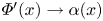
 $\boldsymbol {\nabla }\times \boldsymbol {B}=\alpha \boldsymbol {B}$ with constant
 $\alpha$), which have been shown to be stable to wide class of perturbations (Woltjer Reference Woltjer1958; Molodensky Reference Molodensky1974; Moffatt Reference Moffatt1986). East et al. (Reference East, Zrake, Yuan and Blandford2015) have shown that it is often, perhaps always, possible to find ideal perturbations that decrease the total energy. Whether there are any non-trivial cases of periodic magnetostatic equilibria that are stable is an open question. We provide a review of the instability of linear force-free equilibria in appendix A. The theory that we develop here applies to the idealised stable case, or to the case where viscous damping (which proceeds via motions at the scale of the tangled field) is sufficient to delay the onset of the instability.
In § 4, we present the first (to our knowledge) numerical simulations of isotropic magnetoelasticity. We introduce a sinusoidal velocity perturbation to periodic magnetostatic equilibria, and measure the evolution of the induced standing waves. The results are in excellent agreement with the predictions of our mean-field-theory treatment.
2. A perfectly homogeneous tangle
The equations of ideal (non-resistive), incompressible MHD are
 \begin{gather} \frac{\partial \boldsymbol{u}}{\partial t} + \boldsymbol{u}\boldsymbol{\cdot}\boldsymbol{\nabla}\boldsymbol{u}=-\boldsymbol{\nabla} P + \boldsymbol{B}\boldsymbol{\cdot}\boldsymbol{\nabla}\boldsymbol{B} + \nu\nabla^{2} \boldsymbol{u}, \end{gather}
 \begin{gather}\frac{\partial \boldsymbol{B}}{\partial t} +\boldsymbol{u}\boldsymbol{\cdot}\boldsymbol{\nabla}\boldsymbol{B} = \boldsymbol{B}\boldsymbol{\cdot}\boldsymbol{\nabla}\boldsymbol{u}, \end{gather}
 \begin{gather}\boldsymbol{\nabla}\boldsymbol{\cdot}\boldsymbol{u} = 0, \end{gather}
 \begin{gather}\boldsymbol{\nabla}\boldsymbol{\cdot}\boldsymbol{B} = 0, \end{gather}
where  $P$ is the total (thermal + magnetic) pressure, determined by (2.3);
 $\nu$ is the kinematic viscosity;
 $\boldsymbol {u}$ is the fluid velocity; and the magnetic field
 $\boldsymbol {B}$ is measured in velocity units.
For our purposes, it is convenient to eliminate  $\boldsymbol {B}$ from these equations in favour of the Maxwell stress,
 $M_{ij} = B_i B_j$. Then, in index notation, (2.1) becomes
 \begin{equation} \partial_{\rm t} u_i + u_j\partial_j u_i=-\partial_i P + \partial_j M_{ij}+ \nu \partial_j \partial_j u_i, \end{equation}
while taking the outer product of (2.2) with  $\boldsymbol {B}$ gives
 \begin{equation} \partial_{\rm t} M_{ij} = \mathcal{D}_{ij} \left( M , u \right)\equiv M_{ik}\partial_k u_j + M_{jk}\partial_k u_i - u_k \partial_k M_{ij}, \end{equation}
where  $\mathcal {D}_{ij}(M,u)$ is the (negative) spatial part of the Lie derivative of
 $M$ with respect to
 $\boldsymbol {u}$ – it is the bilinear operator that gives the rate of change of the tensor
 $M$ frozen into the flow
 $\boldsymbol {u}$.
This rewriting of the MHD equations is possible only because we have assumed non-resistive MHD; it would not be possible to write a closed system of evolution equations for  $\boldsymbol {u}$ and
 $M$ if there were a resistive term of the form
 $\eta \nabla ^2 \boldsymbol {B}$ in (2.2). Physically, this is because non-resistive MHD is insensitive to the directed nature of magnetic field lines. This is manifest in the fact the Maxwell stress
 $B_i B_j$ is unchanged by a reversal of the sign of
 $\boldsymbol {B}$. Magnetic diffusion is, of course, sensitive to such direction reversals; a magnetic-field configuration with a sudden direction reversal can be subject to resistive instabilities.
A simple model of a tangled equilibrium state is obtained by linearising (2.5) and (2.6) about the equilibrium state  $M_{ij}= v_E^2\delta _{ij}$, where
 $v_E$ is a constant. A small amount of algebra yields
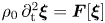
 \begin{equation} \frac{\partial^2 \boldsymbol{\xi}}{\partial t^2} = v_E^2 \nabla^2 \boldsymbol{\xi} + \nu \nabla^2 \frac{\partial \boldsymbol{\xi}}{\partial t}, \end{equation}
where  $\boldsymbol {\xi }$ is the displacement field defined by
 $\partial _{\rm t} \boldsymbol {\xi } = \boldsymbol {u}$. This is a wave equation for (viscously damped) magnetoelastic waves with wave speed
 $v_E$, i.e. waves whose restoring force is the isotropic elasticity of the tangled magnetic field. The corresponding dispersion relation is
 \begin{equation} \omega = {\pm}k v_E \sqrt{1+\left(\frac{\nu k}{2 v_E}\right)^2} - \frac{1}{2}\textrm{i}\nu k^2. \end{equation}
In the absence of viscosity, magnetoelastic waves have dispersion relation  $\omega = {\pm }k v_E$, and can be thought of as the isotropic equivalent of Alfvén waves. Like Alfvén waves, magnetoelastic waves are transverse, as
 $\boldsymbol {\nabla }\boldsymbol {\cdot } \boldsymbol {u} = 0$ implies
 $\boldsymbol {k}\boldsymbol {\cdot }\boldsymbol {\xi }=0$.
The dispersion relation (2.8) was first obtained via a similar derivation by Moffatt (Reference Moffatt1986), and later by Gruzinov & Diamond (Reference Gruzinov and Diamond1996). However, it is an idealisation because no vector field can satisfy  $B_i B_j \propto \delta _{ij}$ at all scales. In the next section, we develop a theory of magnetoelastic waves for a magnetic tangle that is homogeneous and isotropic at large scales, but accounting for its inhomogeneous small-scale structure, and, therefore, the possibility of generating motions at the scale of the magnetic tangle. We find that thedispersion relation (2.8) is modified by a factor of order unity, even in the limit that the magnetic tangle scale is vanishingly small compared with the scale of the magnetoelastic wave.
3. Analytic theory of an inhomogeneous tangle
Returning to the MHD equations, we now separate all quantities into large- and small-scale parts, assuming a scale separation between the typical scales of the wave motions and the magnetic tangle. We denote the wavenumbers associated with these scales by  $k_{\rm w}$ and
 $k_{\rm t}$, respectively, and take
 $k_{\rm w} / k_{\rm t} \equiv \epsilon$ to be a small parameter. We use the notation
 $X = \bar {X} + \tilde {X}$, where
 $\bar {X}$ is the spatial average of the quantity
 $X$ over some intermediate scale that is large compared with the scale of the tangle but small compared with the scale of the wave motion, and
 $\tilde {X}$ is the remaining small-scale part.
Denoting equilibrium fields by a subscript zero, we linearise (2.5) and (2.6) about a static equilibrium that satisfies
 \begin{equation} \bar{M}_{0ij}\equiv v_E^2 \delta_{ij} \end{equation}
for constant  $v_E$, while for the moment remaining agnostic about the form of
 $\tilde {M}_{0ij}$, but expecting that
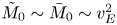 $\tilde {M}_0 \sim \bar {M}_0 \sim v_E^2$ because locally there may be an deviation of order unity of the Maxwell stress from its large-scale average. According to this definition, we have
 $v_E^2 = \overline {v_A^2}/3$, where
 $v_A=v_A(\boldsymbol {r})$ is the local Alfvén speed, i.e. the speed at which small-scale Alfvén waves would propagate along the local magnetic field.
Equation (3.1) implies that the equilibrium Maxwell stress has no structure on the scale of wave motions, therefore our treatment precludes the possibility of treating stochastic fields with structure on all length scales. We note that, while it is possible to generate a wide class of synthetic stochastic magnetic fields satisfying (3.1), this assumption may prove too restrictive to model the fields generated by isotropic MHD turbulence. We shall address this and other differences with the turbulent case in a future publication.
The linearised equations are
 \begin{gather} \partial_{\rm t}^2 \bar{\xi}_i = -\partial_i \bar{P} + v_E^2 \partial_j \partial_j \bar{\xi}_i + \partial_j \bar{\mathcal{D}}_{ij} \left( \tilde{M}_0 , \tilde{\xi} \right) + \nu \partial_j \partial_j \partial_{\rm t} \bar{\xi}_i, \end{gather}
 \begin{gather} \partial_{\rm t}^2 \tilde{\xi}_i = - \partial_i \tilde{P} + v_E^2 \partial_j \partial_j \tilde{\xi}_i + \partial_j \mathcal{D}_{ij} \left( \tilde{M}_0 , \bar{\xi} \right) + \partial_j \tilde{\mathcal{D}}_{ij} \left( \tilde{M}_0 , \tilde{\xi} \right) + \nu \partial_j \partial_j \partial_{\rm t} \tilde{\xi}_i. \end{gather}
3.1. The coupling to small scales is always formally non-negligible
Let us first ask whether it is possible to find a regime in which the coupling to small scales caused by the  $\partial _j \bar {\mathcal {D}}_{ij} ( \tilde {M}_0 , \tilde {\xi } )$ term in (3.2) can be neglected in comparison with the isotropic restoring force
 $v_E^2 \partial _j \partial _j \bar {\xi }_i$. This would require
 $k_{\rm t}\,\tilde {\xi } \ll k_{\rm w}\,\bar {\xi }$, i.e.
 $\tilde {\xi } \ll \epsilon \, \bar {\xi }$. Under this ordering, there are no terms in (3.3) that can balance
 $\partial _j \mathcal {D}_{ij} ( \tilde {M}_0 , \bar {\xi } )$ apart from the viscous term. Such a balance implies
 \begin{equation} k_{\rm w} k_{\rm t} v_E^2 \bar{\xi} \sim \nu k_{\rm t}^2 \,\omega \tilde{\xi} \ll \nu k_{\rm t}^2 \,\omega \epsilon\, \bar{\xi}, \end{equation}
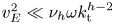
i.e.  $v_E^2 \ll \nu \omega$. Assuming that the large-scale response is indeed elastic gives
 $\omega \sim k_{\rm w} v_E$ as before, which leaves us with
 $v_E \ll \nu k_{\rm w}$. However, this is precisely the condition for the magnetoelastic wave's viscous damping rate to be large compared with the wave frequency, a contradiction to the assumed scaling
 $\omega \sim k_{\rm w} v_E$. Hence we find that the coupling to small scales is always non-negligible if the field is to respond elastically, i.e. if
 $\omega \sim k_{\rm w} v_E$.
This conclusion is a result of the arithmetics of powers of  $k$ in each of the terms in (3.2) and (3.3): essentially, viscosity with its
 $k^2$ scaling does not ‘switch on’ fast enough at larger
 $k$ to prevent the driving of dynamically important small-scale motions. Quenching them requires a viscous damping that scales with
 $k$ faster than
 $k^2$, i.e. a hyperviscosity.Footnote 1 In § 4.3.1, we will present numerical experiments with tangle scales hyperviscously damped, which do indeed show precise agreement with (2.8).
That the coupling to small scales should be formally non-negligible is, in fact, clear on intuitive physical grounds; a set of disconnected ‘blobs’ of magnetic field may well satisfy  $\bar {M}_{0ij} \propto \delta _{ij}$, but will not be able to support a net tension on scales much larger than the typical blob size. In this case, the term describing the coupling to small scales
 $\partial _j \bar {\mathcal {D}}_{ij} ( \tilde {M}_0 , \tilde {\xi } )$ in (3.2) will be non-negligible and its effect will be to cancel the large-scale elasticity term,
 $v_E^2 \partial _j \partial _j \bar {\xi }_i$. This intuition also suggests that the effect of the coupling to small scales should reduce the effective elasticity, an expectation that is confirmed by the analysis in the next section. Hyperviscosity modifies this picture by preventing any differential motion on small scales, so the fluid behaves as though the magnetic blobs were connected by rigid rods that allow the large-scale tension to be maintained.
3.2. Normal-mode analysis
Some general statements can be made regarding the elastic response of an inviscid tangle by conducting a normal-mode analysis. The essential result of this section is that for a stable field configuration, the frequency of magnetoelastic waves is always decreased from  $k_{\rm w} v_E$ as a result of intermittency of the Maxwell stress.
We expand the displacement field and Maxwell stress in Fourier modes, viz.,  $\xi _i=\sum _{\boldsymbol {k}} \xi _i(\boldsymbol {k})\exp ({\textrm {i}(\boldsymbol {k}\boldsymbol {\cdot }\boldsymbol {r}-\omega t)})$ and
 $M_{0ij}=\sum _{\boldsymbol {k}} M_{0ij}(\boldsymbol {k})\exp ({\textrm {i}\boldsymbol {k}\boldsymbol {\cdot }\boldsymbol {r}})$, define the projection operator
 $\mathcal {P}_{ij}(\boldsymbol {k})=\delta _{ij}-k_i k_j/k^2$, and define the matrix elements
 $A_{ij}(\boldsymbol {k}, \boldsymbol {k}')$ of the operator
 $\mathcal {P}_{il}\partial _j \mathcal {D}_{lj} ( M_0 , \bullet )$ in the Fourier basis so that
 \begin{equation} -\omega^2 \xi_i(\boldsymbol{k}) = \sum_{\boldsymbol{k}'} A_{ij}(\boldsymbol{k}, \boldsymbol{k}') \xi_j(\boldsymbol{k}'). \end{equation}
The explicit form of  $A_{ij}(\boldsymbol {k}, \boldsymbol {k}')$ can be obtained straightforwardly from the definition (2.6) of
 $\mathcal {D}$, viz.,
 \begin{align} &A_{in}(\boldsymbol{k}, \boldsymbol{k}') = - \mathcal{P}_{il}\left(\boldsymbol{k}\right)k_j \left[-\left(k_m-k'_m\right) M_{0lj}\left(\boldsymbol{k}-\boldsymbol{k}'\right)\mathcal{P}_{mn}\left(\boldsymbol{k}'\right) \right.\nonumber\\ &\quad + \left. M_{0lm}\left(\boldsymbol{k}-\boldsymbol{k}'\right)k_m' \mathcal{P}_{jn}\left(\boldsymbol{k}'\right)+M_{0jm}\left(\boldsymbol{k}-\boldsymbol{k}'\right)k_m' \mathcal{P}_{ln}\left(\boldsymbol{k}'\right)\right]. \end{align}
Importantly,  $A_{ij}(\boldsymbol {k}, \boldsymbol {k}')$ is Hermitian, i.e.
 $A_{ij}(\boldsymbol {k}, \boldsymbol {k}')=[ A_{ji}(\boldsymbol {k}', \boldsymbol {k}) ]^{*}$.Footnote 2 Let us prove this explicitly. The Hermitian conjugate of (3.6) is
 \begin{align} \left[ A_{ni}(\boldsymbol{k}', \boldsymbol{k}) \right]^{*} & = - \mathcal{P}_{nl}\left(\boldsymbol{k}'\right)k_j' \left[-\left(k'_m-k_m\right) M_{0lj}\left(\boldsymbol{k}-\boldsymbol{k}'\right)\mathcal{P}_{mi}\left(\boldsymbol{k}\right) \right.\nonumber\\ &\quad + \left. k_m M_{0lm}\left(\boldsymbol{k}-\boldsymbol{k}'\right) \mathcal{P}_{ji}\left(\boldsymbol{k}\right)+k_m M_{0jm}\left(\boldsymbol{k}-\boldsymbol{k}'\right) \mathcal{P}_{li}\left(\boldsymbol{k}\right)\right]. \end{align}
Taking  $m\leftrightarrow l$ in the first term of (3.6), and
 $j\leftrightarrow l$ in the second term, then subtracting (3.7) from (3.6) gives
 \begin{align} & A_{in}(\boldsymbol{k}, \boldsymbol{k}') -\left[ A_{ni}(\boldsymbol{k}', \boldsymbol{k}) \right]^{*}\nonumber\\ &\quad = \mathcal{P}_{il}\left(\boldsymbol{k}\right) \mathcal{P}_{nj}\left(\boldsymbol{k}'\right)\left(\delta_{lp}\delta_{jq}-\delta_{lq}\delta_{jp}\right) \left(k_q-k'_q\right) \left(k_m-k'_m\right) M_{0pm}\left(\boldsymbol{k}-\boldsymbol{k}'\right), \end{align}
which is zero, as  $\delta _{lp}\delta _{jq}-\delta _{lq}\delta _{jp}$ =
 $\epsilon _{rlj}\epsilon _{rpq}$, and
 $\epsilon _{rpq} (k_q-k'_q)(k_m-k'_m) M_{0pm}(\boldsymbol {k}- \boldsymbol {k}') = 0$ because the equilibrium field must satisfy
 $\boldsymbol {\nabla }\times (\boldsymbol {\nabla }\boldsymbol {\cdot }\boldsymbol {M}_0)=0$ (see equation 2.5). Therefore,
 $A_{ij}(\boldsymbol {k}, \boldsymbol {k}')=[ A_{ji}(\boldsymbol {k}', \boldsymbol {k}) ]^{*}$, q.e.d.
When  $\boldsymbol {k}'=\boldsymbol {k}$, (3.6) reduces to
 $A_{ij}(\boldsymbol {k}, \boldsymbol {k})=-M_{0ll}(\boldsymbol {0})k^2 \delta _{ij}=-k^2v_E^2 \delta _{ij}$, so each Fourier mode is subject to the large-scale isotropic restoring force, as in (3.3). Terms with
 $\boldsymbol {k}'\neq \boldsymbol {k}$ describe the coupling of different Fourier modes; indeed, from (3.6), we see that Fourier modes of the displacement field
 $\boldsymbol {\xi }$ with wavevectors
 $\boldsymbol {k}$ and
 $\boldsymbol {k}'$ are coupled to each other only when
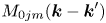 $M_{0jm}(\boldsymbol {k}-\boldsymbol {k}')$ is non-zero. This observation shows that two large-scale Fourier modes with
 $\boldsymbol {k}, \boldsymbol {k}'\sim k _{\rm w}$ are not coupled by (3.6), because
 $M_{0ij}(\boldsymbol {k})=0$ for
 $\boldsymbol {k}\sim k _{\rm w}$, by (3.1). In principle, these large-scale Fourier modes can still be coupled as a result of each of them coupling individually to small scales. The condition for two large-scale Fourier modes to be coupled in this way is the existence of a path in Fourier space between them, along the wavevectors of
 $M_0$. This is precisely the condition for the Fourier modes of
 $M_0$ to ‘beat’ at the magnetoelastic-wave scale, which is in contradiction to the assumption of statistical homogeneity at large scales. Henceforth, we will assume that such beating is absent from
 $M_0$, and, therefore, that different large-scale Fourier modes are completely decoupled.Footnote 3 We will also assume that large-scale modes with the same
 $\boldsymbol {k}$ but different spatial directions are decoupled, which is a natural consequence of statistical isotropy. This discussion implies that it is sensible to decompose the large-scale perturbation into its constituent Fourier modes, each of which will independently drive small-scale motions that feed back on the particular large-scale Fourier mode that caused them, but not on any other large-scale modes.
If we take  $M_0$ to have a finite number of non-zero Fourier modes,Footnote 4 then
 $A_{ij}(\boldsymbol {k}, \boldsymbol {k}')$ can be considered as a Hermitian matrix whose elements
 $A_{(\boldsymbol {k}, i)(\boldsymbol {k}',\, j)}$ describe the coupling of the mode
 $\xi _i (\boldsymbol {k})$ with
 $\xi _j (\boldsymbol {k}')$. Since a large-scale mode may couple to small-scale modes but not to other large-scale modes, the matrix representation of
 $A$ is block diagonal, with each block corresponding to one particular large-scale mode and the small-scale modes to which it couples. Let
 $\mathcal {A}$ be the block of size
 $(N+1)\times (N+1)$ corresponding to a particular large-scale mode
 $\xi _z (\boldsymbol {k}_{\rm w})$, taken to be in the
 $z$-direction without loss of generality, that is coupled to
 $N$ small-scale modes. The general structure of
 $\mathcal {A}$ is
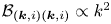
 \begin{equation} \mathcal{A} = \begin{pmatrix} -k_{\rm w}^2 v_E^2 & \boldsymbol{f}^{\dagger}\\ \boldsymbol{f} & \mathcal{B} \end{pmatrix}, \end{equation}
where the element  $\mathcal {A}_{(\boldsymbol {k}_{\rm w}, z)(\boldsymbol {k}_{\rm w}, z)}\equiv A_{zz}(\boldsymbol {k}_{\rm w}, \boldsymbol {k}_{\rm w})=- k_{\rm w}^2 v_E^2$ describes the isotropic elastic restoring force on the large-scale mode;
 $\mathcal {A}_{(\boldsymbol {k}, i)(\boldsymbol {k}_{\rm w}, z)}\equiv A_{iz}(\boldsymbol {k}, \boldsymbol {k}_{\rm w})\equiv f_{(\boldsymbol {k}, i)}$ for
 $|\boldsymbol {k}|\sim k_{\rm t}$ is an
 $N$-dimensional vector that gives the coupling of the small-scale modes to the large-scale mode; and
 $\mathcal {A}_{(\boldsymbol {k}, i)(\boldsymbol {k}', j)}\equiv A_{ij}(\boldsymbol {k},\boldsymbol {k}')\equiv \mathcal {B}_{(\boldsymbol {k}, i)(\boldsymbol {k}', j)}$ for
 $|\boldsymbol {k}|,\,|\boldsymbol {k}'|\sim k _{\rm t}$ is the
 $N\times N$ Hermitian matrix representing the coupling of the relevant small-scale modes to each other. The sizes of these three components are, respectively,
 $k_{\rm w}^2 v_E^2$,
 $k_{\rm w} k_{\rm t} v_E^2$ and
 $k_{\rm t}^2 v_E^2$.
The  $N+1$ normal modes of the system have frequencies
 $\omega _{\mu }$ that satisfy
 $\det (\mathcal {A}+\omega _{\mu }^2 I_{N+1})=0$, where
 $I_{N+1}$ is the identity matrix of size
 $N+1$. To leading order in
 $\epsilon$, the fast, small-scale motions with frequency
 $\omega _{\mu }\sim k_{\rm t} v_E$ satisfy
 \begin{equation} \det \begin{pmatrix} \omega_{\mu}^2 & \boldsymbol{f}^{\dagger}\\ \boldsymbol{f} & \mathcal{B} + \omega_{\mu}^2 I_N \end{pmatrix}= \omega_{\mu}^2 \det \left(\mathcal{B}+\omega_{\mu}^2 I_N\right)=0\implies \det \left(\mathcal{B}+\omega_{\mu}^2 I_N\right)=0, \end{equation}
so that the fast frequencies are unaffected by the coupling of large and small scales. Equation (3.10) has  $N$ solutions for
 $\omega _{\mu }^2$, which we denote by
 $\mu =1,\ldots ,N$. The remaining slow, large-scale solution with frequency
 $\omega _0\sim k _{\rm w} v_E$ represents a magnetoelastic wave, and satisfies
 \begin{equation} \det \begin{pmatrix} \omega_0^2- k_{\rm w}^2 v_E^2 & \boldsymbol{f}^{\dagger}\\ \boldsymbol{f} & \mathcal{B} \end{pmatrix}=0. \end{equation}
Defining the block matrix
 \begin{equation} T=\begin{pmatrix} 1 & 0\\ 0 & U \end{pmatrix}, \end{equation}
where  $U$ is the
 $N\times N$ unitary matrix that diagonalises the matrix
 $\mathcal {B}$, and using the invariance of the determinant under the basis transformation defined by
 $T$, we obtain
 \begin{equation} \det \begin{pmatrix} \omega_0^2- k_{\rm w}^2 v_E^2 & \left(U\boldsymbol{f}\right)^{\dagger}\\ U\boldsymbol{f} & \varLambda \end{pmatrix}=0,\end{equation}
where  $\varLambda =U\mathcal {B}\,U^{\dagger}=\text {diag}(\lambda _1, \ldots ,\lambda _N )=\text {diag}(-\omega _1^2, \,\dots ,-\omega _N^2 )$ is the diagonal matrix of eigenvalues of
 $\mathcal {B}$, which are the
 $N$ (negative squared) frequencies of the small-scale system. Since
 $\varLambda$ is diagonal, the determinant is simple to evaluate, and (3.13) leads to
 \begin{equation} \omega_0^2 = k_{\rm w}^2 v_E^2 - \sum_{\mu=1}^N \frac{\large|(U \boldsymbol{f})_{\mu}\large|^2}{\omega_{\mu}^2}. \end{equation}
Equation (3.14) shows that the effect of the coupling to small-scale motions is to reduce the frequency of large-scale waves, as long as the equilibrium is stable, i.e. as long as all  $\omega _{\mu }^2>0$. Furthermore, since the components of
 $U$ and
 $\boldsymbol {f}$ are
 ${\sim }1$ and
 ${\sim }k_{\rm w} k_{\rm t} v_E^2$, respectively, while
 $\omega _{\mu }\sim k_{\rm t} v_E$ for
 $\mu \geq 1$, the frequency is reduced by a factor of order unity. Physically, this is akin to the elastic response of a tangled ball of elastic string compared with a solid elastic block: a deformation will generally produce a smaller restoring force in the elastic ball because the strings can move relative to each other to reduce the elastic energy (this is not possible in a hyperviscous fluid as small-scale motions are suppressed).
Of course, there is no reason that the right-hand side of (3.14) should be positive; if it is not, (3.14) describes a growing perturbation at large scales. This result shows that it is in principle possible for an unstable magnetic tangle to relax via motions on large scales rather than small scales. However, we have found no example of this in our numerical studies, where the effect of the tangled field on large-scale modes was always restoring, with instability proceeding only via motions at small scales.
The eigenvectors of  $\mathcal {A}$ can be obtained to leading order by noting that
 $\mathcal {A} (0, \boldsymbol {e}_{\mu })^{\text {T}} = \lambda _{\mu }(0, \boldsymbol {e}_{\mu })^{\text {T}} + O(\epsilon )$, where
 $\boldsymbol {e}_{\mu }$ is the
 $\mu$th eigenvector of the matrix
 $\mathcal {B}$. The final eigenvector with associated frequency
 $\omega _0$ is uniquely constrained by orthogonality to be
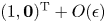 $(1, \boldsymbol {0})^{\text {T}}+O(\epsilon )$. Therefore, a magnetoelastic wave consists primarily of a large scale oscillation, together with small-amplitude (vanishing as
 $\epsilon \rightarrow 0$), slow (frequency
 $\omega _0$), small-scale oscillations. Physically, these small-scale oscillations represent the rearrangement of small-scale structures to reduce the elastic energy and, therefore, the large-scale tension. Despite having small amplitude, these small-scale motions are by no means negligible – as we have found, the magnetoelastic wave frequency is changed by a factor of order unity in their absence.
3.3. The FOSA
In this section, we describe an approximate method to obtain the wave frequency  $\omega _0$ in terms of statistical properties of the magnetic tangle, by assuming that the coupling between different small-scale Fourier modes is small. This approximation is equivalent to neglecting the term
 $\partial _j \tilde {\mathcal {D}}_{ij} ( \tilde {M}_0 , \tilde {\xi })$ in (3.3); in the context of large-scale kinematic dynamo theory, it is often called the first-order smoothing approximation (FOSA) or the second-order correlation approximation (SOCA). In the dynamo-theory context, it is employed in the small-scale part of the induction equation to neglect a similar ‘fluctuating part of the product of two fluctuations’ term, allowing the small-scale induction equation to be solved for the small-scale magnetic field, which can then be used to compute the growth of the large-scale field (for a review, see Rincon (Reference Rincon2019)). Our use of this approximation is directly complementary: instead of solving an equation for the small-scale magnetic field given a prescribed flow, we use the FOSA to solve an equation for a small-scale flow given a known small-scale magnetic-field configuration,
 $M_0$.
Much like in the dynamo-theory context, where the FOSA is rigorously justified only when either the velocity correlation time is small, or  $\mathrm {Rm}\ll 1$, the assumption of weak coupling between modes is unlikely to be well satisfied in any real magnetic tangle. However, the FOSA remains a useful tool, and we show in § 4 that it provides a remarkably good description of numerical simulations of large-scale waves in tangled-magnetic-field equilibria.
Under the FOSA, we neglect all off-diagonal terms of the matrix  $\mathcal {B}$ in (3.11), so that the coupling of large and small scales is retained, but the small-scale modes do not couple to each other. This simplifies (3.14) considerably because now
 $U=I_N$ and
 $\omega _{\mu }= k_{\mu } v_E$ for
 $\mu =1,\ldots ,N$, where
 $k_{\mu }$ are the wavenumbers of the
 $N$ small-scale modes, so that (3.14) becomes
 \begin{equation} \omega_0^2 = k^2 v_E^2 - \sum_{\boldsymbol{k}'\neq\boldsymbol{k}_{\rm w}} \frac{A_{zp}(\boldsymbol{k}_{\rm w}, \boldsymbol{k}')A_{pz}(\boldsymbol{k}', \boldsymbol{k}_{\rm w}) }{k'^2 v_E^2}. \end{equation}
With  $i \rightarrow z$ and
 $\boldsymbol {k}\rightarrow \boldsymbol {k}_{\rm w}$, (3.6) gives
 \begin{align} A_{zn}(\boldsymbol{k}_{\rm w}, \boldsymbol{k}') &= - \mathcal{P}_{zl}\left(\boldsymbol{k}_{\rm w}\right)k_{{\rm w}j} \left[-\left(k_{{\rm w}m}-k'_{m}\right) M_{0lj}\left(\boldsymbol{k}_{\rm w}-\boldsymbol{k}'\right)\mathcal{P}_{mn}\left(\boldsymbol{k}'\right) \right.\nonumber\\ &\quad + \left. M_{0lm}\left(\boldsymbol{k}_{\rm w}-\boldsymbol{k}'\right)k_m' \mathcal{P}_{jn}\left(\boldsymbol{k}'\right)+M_{0jm}\left(\boldsymbol{k}_{\rm w}-\boldsymbol{k}'\right)k_m' \mathcal{P}_{ln}\left(\boldsymbol{k}'\right)\right]. \end{align}
With  $|\boldsymbol {k}'| \sim k_{\rm t}$, the first term in the square brackets vanishes to leading order in
 $\epsilon$ because
 $k'_m \mathcal {P}_{mn}(\boldsymbol {k}')=0$. Relabelling
 $n\rightarrow p$, then swapping
 $m\leftrightarrow j$ and
 $m\leftrightarrow l$ in the second term, we obtain
 \begin{align} A_{zp}(\boldsymbol{k}_{\rm w}, \boldsymbol{k}') &= - \mathcal{P}_{zl}\left(\boldsymbol{k}_{\rm w}\right)k_{{\rm w}m} M_{0lj}\left(\boldsymbol{k}_{\rm w}-\boldsymbol{k}'\right)k_j' \mathcal{P}_{mp}\left(\boldsymbol{k}'\right)\nonumber\\ &\quad-\mathcal{P}_{zm}\left(\boldsymbol{k}_{\rm w}\right)k_{{\rm w}j} M_{0jl}\left(\boldsymbol{k}_{\rm w}-\boldsymbol{k}'\right)k_l' \mathcal{P}_{mp}\left(\boldsymbol{k}'\right)\nonumber\\ &= - k_{{\rm w}n} k_l' \mathcal{P}_{zq}\left(\boldsymbol{k}_{\rm w}\right)\mathcal{P}_{mp}\left(\boldsymbol{k}'\right)\left(\delta_{nm}\delta_{jq}+\delta_{nj}\delta_{mq}\right)M_{0lj}\left(\boldsymbol{k}_{\rm w}-\boldsymbol{k}'\right). \end{align}
An analogous expression for  $A_{pz}(\boldsymbol {k}', \boldsymbol {k}_{\rm w})$ can be obtained directly from (3.7), but the derivation is much more involved. Instead, we can use the fact that
 $A$ is Hermitian:
 \begin{align} A_{pz}(\boldsymbol{k}', \boldsymbol{k}_{\rm w})&=\left[A_{zp}(\boldsymbol{k}_{\rm w}, \boldsymbol{k}')\right]^{*}\nonumber\\ &=- k_{{\rm w}n} k_l' \mathcal{P}_{zq}\left(\boldsymbol{k}_{\rm w}\right)\mathcal{P}_{mp}\left(\boldsymbol{k}'\right)\left(\delta_{nm}\delta_{jq}+\delta_{nj}\delta_{mq}\right)M_{0lj}\left(\boldsymbol{k}'-\boldsymbol{k}_{\rm w}\right)\nonumber\\ & =- k_{{\rm w}n} k_j' \mathcal{P}_{zm}\left(\boldsymbol{k}_{\rm w}\right)\mathcal{P}_{qp}\left(\boldsymbol{k}'\right)\left(\delta_{nq}\delta_{lm}+\delta_{nl}\delta_{mq}\right)M_{0lj}\left(\boldsymbol{k}'-\boldsymbol{k}_{\rm w}\right), \end{align}
where to obtain the final expression we have swapped  $l \leftrightarrow j$ and
 $q \leftrightarrow m$.
With (3.17) and (3.18), (3.15) becomes
 \begin{equation} \omega_0^2 = k_{\rm w}^2 v_E^2 - \left(\delta_{nm}\delta_{jz}+\delta_{nj}\delta_{mz}\right)\left(\delta_{zl'}\delta_{n'q'}+\delta_{l'n'}\delta_{zq'}\right)k_{{\rm w}n} k_{{\rm w}n'}R_{mq'jl'}, \end{equation}
where
 \begin{equation} R_{mq'jl'}=\sum_{\boldsymbol{k}'} \frac{k_l' k_{j'}'}{k'^2 v_E^2} \mathcal{P}_{q'm}\left(\boldsymbol{k}'\right)\tilde{M}_{lj}\left(-\boldsymbol{k}'\right) \tilde{M}_{l'j'}\left(\boldsymbol{k}'\right), \end{equation}
to leading order in  $\epsilon$. The rank-four tensor
 $R_{pq'jl'}$ is a statistical property (in the sense of volume averaging) of the magnetic tangle. Since we have assumed statistical isotropy, the most general form it can take is
 $R_{pq'jl'}=a\delta _{pq'}\delta _{jl'}+b\delta _{pj}\delta _{q' l'}+c\delta _{pl'}\delta _{q'j}$. Noting from (3.20) that
 $R_{pq'jl'}$ is symmetric in
 $p$ and
 $q'$ and vanishes on contraction of
 $p$ with
 $l'$, we find
 \begin{equation} R_{pq'jl'}=\frac{1}{30v_E^4}\left(4\delta_{l'j}\delta_{pq'}-\delta_{l'p}\delta_{jq'}-\delta_{l'q'}\delta_{jp}\right)\left(\left\langle P_0^2\right\rangle - \left\langle P_0\right\rangle^2\right). \end{equation}
where we have used the equilibrium condition  $k_j M_{0ij}(\boldsymbol {k}) + k_i P_0(\boldsymbol {k})=0$, where
 $P_0$ is the equilibrium total pressure distribution, and identified
 \begin{equation} \sum_{\boldsymbol{k}'}\left|\tilde{P}_0 \left(\boldsymbol{k}'\right)\right|^{2} = \left \langle P_0^2 \right \rangle - \left \langle P_0 \right \rangle^2, \end{equation}
where angled brackets indicate spatial averages. On substitution of this result into (3.19) and contraction of the many Kronecker deltas, we finally arrive at
 \begin{equation} \omega_0^2 = k^2 v_E^2\left(1-\chi\right), \end{equation}
where
 \begin{equation} \chi = \frac{1}{5v_E^4}\left(\left\langle P_0^2\right\rangle - \left\langle P_0\right\rangle^2\right). \end{equation}
We therefore find that under the FOSA, the effect of the small-scale structure of the magnetic tangle is to reduce the frequency of magnetoelastic waves by an amount proportional to the variance of the total pressure. This is really a statement about the magnetic field, since the total pressure must balance the magnetic tension force in equilibrium, so (3.24) shows that more intermittent magnetic fields are less elastic. This is precisely in agreement with the intuitive reasoning of § 3.1, where we argued that a field configuration consisting of disconnected magnetic ‘blobs’ would not support a large-scale tension – such a field would have a large value of  $\chi$.
In the special case of a force-free magnetic tangle, i.e. when only magnetic pressure balances the magnetic tension,  $P_0=B_0^2/2$, so
 \begin{equation} \chi = \frac{9}{20}\left(\frac{\left\langle B_0^4\right\rangle}{\left\langle B_0^2\right\rangle^2} - 1\right). \end{equation}
Like (3.14), (3.23) permits an instability on large scales, occurring when  $\chi >1$. Note that the FOSA treats the small-scale system as stable; this is a consequence of neglecting the off-diagonal terms in the matrix
 $\mathcal {B}$. Formally, therefore, the FOSA predicts that when the variance of the total pressure becomes large enough (so that
 $\chi >1$), a statistically homogeneous and isotropic magnetic tangle can be unstable to large-scale perturbations, even while remaining stable to those with scale similar to that of the tangle itself. This prediction is contrary to the intuitive picture that we have developed so far. Consider again a set of disconnected magnetic blobs. While it is intuitive that this configuration should not produce an elastic response to a large-scale perturbation, it is not clear that increasing the variance of the field strength (e.g. by reducing the size of the blobs while increasing their field strength to maintain a constant spatial average) should introduce an instability, causing the large-scale perturbation to grow. The source of the discrepancy between formalism and physical intuition is that strongly intermittent configurations with large
 $\chi$ are poorly described by the FOSA. From (3.15), we see that
 $\chi$ can be thought of as a measure of the strength of the coupling between large and small scales. When this coupling is strong (large
 $\chi$), describing the small-scale dynamics accurately is essential to obtaining correct large-scale dynamics. Indeed, in § 4, we show with numerical simulations of linear force-free fields that the FOSA becomes inaccurate for large values of
 $\chi$.
3.4. Magnetoelastic waves in a viscous fluid
In this section, we develop a theory for magnetoelastic waves propagating through a viscous fluid. As we found in § 3.2, a magnetoelastic wave in an inviscid fluid is a large-scale oscillation, accompanied by slow ( $\omega \sim k_{\rm w} v_E$), small-amplitude oscillations associated with the relaxation of small-scale structures in response to the large-scale tension. In the viscous case, these small-scale structures will be damped by viscosity; their presence therefore results in an anomalous viscous damping of magnetoelastic waves.
For definiteness, we take the initial condition to be a large-scale velocity perturbation  $u_z$ along
 $z$ with wavevector
 $\boldsymbol {k}_{\rm w}$. We solve the initial-value problem by taking a Laplace transform in time,
 \begin{equation} p^2 \xi_z(\boldsymbol{k}_{\rm w}) - u_z\left(\boldsymbol{k}_{\rm w},t=0\right) = -k_{\rm w}^2v_E^2 \xi_z(\boldsymbol{k}_{\rm w})+ \sum_{\boldsymbol{k}'} A_{zj}(\boldsymbol{k}_{\rm w}, \boldsymbol{k}') \xi_j(\boldsymbol{k}') +\nu k_{\rm w}^2 p \xi_z(\boldsymbol{k}_{\rm w}), \end{equation}
where  $p$ is the Laplace conjugate variable to time (analogous to
 $\textrm {i}\omega$).
In the FOSA, an initially unperturbed small-scale mode with wavenumber  $k' \gg k_{\rm w}$ satisfies
 \begin{equation} p^2 \xi_j(\boldsymbol{k}') = -v_E^2 k'^2 \xi_j(\boldsymbol{k}') + A_{jz}(\boldsymbol{k}', \boldsymbol{k}_{\rm w}) \xi_z(\boldsymbol{k}_{\rm w}) +\nu k'^2 p \xi_j(\boldsymbol{k}'). \end{equation}
Solving this algebraic equation for  $\xi _j(\boldsymbol {k}')$, and substituting into (3.26), we obtain
 \begin{align} & p^2 \xi_z(\boldsymbol{k}_{\rm w}) - u_z\left(\boldsymbol{k}_{\rm w},t=0\right) =-k_{\rm w}^2v_E^2 \xi_z(\boldsymbol{k}_{\rm w})\nonumber\\ &\quad+ \sum_{\boldsymbol{k}'} \frac{A_{zj}(\boldsymbol{k}_{\rm w}, \boldsymbol{k}') A_{jz}(\boldsymbol{k}', \boldsymbol{k}_{\rm w})}{p^2 + v_E^2 k'^2 + \nu k'^2 p}\xi_z (\boldsymbol{k}_{\rm w}) +\nu k_{\rm w}^2 p \xi_z(\boldsymbol{k}_{\rm w}), \end{align}
where the sum is over all small-scale modes.
With  $p\sim \omega _0\sim k_{\rm w} v_E$, the
 $p^2$ in the denominator of the coupling term in (3.28) is small compared with
 $v_E^2 k'^2$.Footnote 5 Neglecting it, we can use (3.17) and (3.18) analogously to the inviscid case to write
 \begin{equation} p^2 \xi_z(\boldsymbol{k}_{\rm w}) - u_z\left(\boldsymbol{k}_{\rm w},t=0\right) =-k_{\rm w}^2v_E^2 \xi_z(\boldsymbol{k}_{\rm w})+\frac{\chi}{1 + \nu p/v_E^2}k_{\rm w}^2v_E^2\xi_z(\boldsymbol{k}_{\rm w}) +\nu k_{\rm w}^2 p \xi_z(\boldsymbol{k}_{\rm w}). \end{equation}
Note that, as predicted in § 3.1, the term representing coupling to small scales remains finite as  $\epsilon \rightarrow 0$, and can only be neglected when
 $\nu p / v_E^2 \sim \nu k_{\rm w}^2 / k_{\rm w} v_E \gg 1$, i.e. when wave motions are strongly damped. In contrast, in the hyperviscous case, the number of powers of
 $k'$ is increased in the viscosity term in the denominator of the coupling term in (3.28), so that it is sufficient for small scales to be strongly damped for the coupling term to be negligible as
 $\epsilon \rightarrow 0$. We therefore recover the simple wave equation (2.7) in the hyperviscous case, as predicted in § 3.1.
Finally, we invert the Laplace transform using Cauchy's residue theorem. The solution is a sum of Laplace modes  $\bar {u}_i (t) = \left (\sum _n A_n e^{p_n t}\right ) \bar {u}_i (0)$ with amplitudes
 \begin{equation} A_{n} = \text{Res} \left[ \frac{p}{D(p )} , p\rightarrow p_n \right], \end{equation}
where ‘ $\mathrm {Res}$’ denotes the residue and
 $\{p_n\}$ are the roots of the dispersion relation
 \begin{equation} D(p_n) \equiv p_n^2+\left(1-\frac{\chi}{1 + \nu p_n/v_E^2}\right) v_E^2k^2+\nu k^2 p_n = 0. \end{equation}
It is instructive to consider the case where the viscous damping rate is finite but small compared with the wave frequency, i.e.  $\hat {\nu }\equiv \nu k_{\rm w}/v_E\ll 1$. The solutions of (3.31) in this limit are
 \begin{align} p_1 &= +\textrm{i} v_E k_{\rm w} \sqrt{1-\chi} - \tfrac{1}{2}\nu k_{\rm w}^2 \left(1+\chi\right) + O\left(\hat{\nu}^2\right), \end{align}
 \begin{align}p_2 &= -\textrm{i} v_E k_{\rm w} \sqrt{1-\chi} - \tfrac{1}{2}\nu k_{\rm w}^2 \left(1+\chi\right) + O\left(\hat{\nu}^2\right), \end{align}
 \begin{align}p_3 &= -v_E^2 /\nu + O\left(\hat{\nu}\right), \end{align}
with corresponding amplitudes
 \begin{equation} A_{1} = \tfrac{1}{2} + O\left(\hat{\nu}\right), \quad A_{2} = \tfrac{1}{2} + O\left(\hat{\nu}\right), \quad A_{3} = \chi \hat{\nu}^2 + O\left(\hat{\nu}^3 \right). \end{equation}
In the first two solutions,  $p_1$ and
 $p_2$, given by (3.32) and (3.33), we find the wave modes of the previous section, but now with a damping rate that is larger than in the perfectly homogeneous case by a factor of
 $1+\chi$. This increased damping rate is expected: it is a consequence of the viscous damping of the small-scale motions associated with magnetoelastic waves. It may appear odd that a damping associated with small-scale motions has a rate
 $\propto \nu k_{\rm w}^2$, especially as the condition
 $\hat {\nu }\ll 1$ does not exclude the possibility of fast, small scale motions being overdamped by viscosity. The resolution is that the small-scale motions associated with a magnetoelastic wave are slow (frequency
 $\sim k_{\rm w} v_E$), not fast, and therefore they are not viscously dominated when
 $\hat {\nu }\ll 1$, as
 $\nu \partial _j \partial _j \partial _{\rm t} \tilde {\xi }_i\sim \nu k_{\rm t}^2 \omega _0 \tilde {\xi } \sim \hat {\nu }k_{\rm t}^2v_E^2 \tilde {\xi } \ll v_E^2 \partial _j \partial _j \tilde {\xi }_i\sim k_{\rm t}^2v_E^2 \tilde {\xi }$. These motions satisfy the balance
 $v_E^2 \partial _j \partial _j \tilde {\xi }_i \sim \partial _j \mathcal {D}_{ij} ( \tilde {M}_0 , \bar {\xi } )$, which gives
 $\tilde {\xi }\sim \epsilon \bar {\xi }$. The rate of energy dissipation associated with them is therefore
 $\sim \nu k_{\rm t}^2 \omega _0^2 \tilde {\xi }^2\sim \nu k_{\rm w}^2 \omega _0^2 \bar {\xi }$, which is consistent with the anomalous damping rate in (3.32) and (3.33).
The third mode,  $p_3$, given by (3.34), describes the case where the slow, small-scale motions associated with the waves do become viscously dominated, so obey the balance
 $v_E^2 \partial _j \partial _j \tilde {\xi }_i \sim k_{\rm t}^2 \partial _{\rm t} \tilde {\xi }$, giving a damping rate of
 $v_E^2/\nu$. As above, these motions become viscously dominated only when
 $\hat {\nu }\sim 1$, explaining the vanishing amplitude of this mode when
 $\hat {\nu }\ll 1$.Footnote 6
4. Numerical study
4.1. Ideal instability of tangled-magnetic-field equilibria
The analysis in the preceding sections has been idealised because real tangled magnetic equilibria are generically unstable, even to ideal perturbations (Er-Riani, Naji & El Jarroudi Reference Er-Riani, Naji and El Jarroudi2014; East et al. Reference East, Zrake, Yuan and Blandford2015). The instability typically proceeds via motions at small scales that are fast compared with the magnetoelastic wave motions, but are inhibited by the presence of viscosity. However, the growth rate associated with viscously dominated, small-scale unstable modes is  ${\sim }v_E^2/\nu$, which becomes comparable with the wave frequency when
 $\hat {\nu }=\nu k_{\rm w}^2 / k_{\rm w} v_E \sim 1$, i.e. when magnetoelastic waves are strongly damped by viscosity. The question then arises as to whether any static, tangled-magnetic-field equilibrium will persist long enough for waves to propagate through it, even with strong viscosity. In fact, we have found in our numerical study that when the equilibrium state is an linear force-free magnetic field (see next section) the growth rate of the instability is sufficiently slow for the equilibrium configuration to persist for many wave periods.
The existence of an instability of linear force-free magnetic fields in ideal MHD has only recently been appreciated, and indeed many inaccurate statements have historically been presented in the literature. For the interested reader, we present a short review of this instability in appendix A.
4.2. Simulation set-up
In order to test the analytic predictions derived in the previous sections, we conduct simulations of standing magnetoelastic waves on periodic, linear, force-free magnetic-field equilibria with different values of the parameter  $\chi$.
The linear force-free magnetic-field condition is  $\boldsymbol {\nabla }\times \boldsymbol {B}=\alpha \boldsymbol {B}$, where
 $\alpha$ is a constant. Taking the curl and using
 $\boldsymbol {\nabla }\boldsymbol {\cdot }\boldsymbol {B}=0$, we get a Helmholtz equation for the magnetic field,
 $\nabla ^2\boldsymbol {B}=-\alpha ^2 \boldsymbol {B}$, which shows that the modes in the Fourier expansion of
 $\boldsymbol {B}$ must all have
 $|\boldsymbol {k}|=\alpha$. The linear force-free equilibrium must then have
 $\textrm {i} \boldsymbol {k}\times \boldsymbol {B_k} = \alpha \boldsymbol {B_k}$, or
 \begin{equation} \hat{\boldsymbol{k}}\times \text{Re}\left(\boldsymbol{B_k}\right)= \text{Im}\left(\boldsymbol{B_k}\right). \end{equation}
To generate tangled magnetic equilibria, we take  $\boldsymbol {k}L=2{\rm \pi} (12, 6, 0)^{\mathrm {T}}$, together with all its permutations and negations, where
 $L$ is the box size. This means that the magnetic-field structure is periodic on a scale of
 $L/6$, which ensures the scale separation between the box scale and the scale of the tangled field. We then generate real vectors
 $\text {Re}(\boldsymbol {B_k})$ subject to the condition
 $\text {Re}(\boldsymbol {B_k})= \text {Re}(\boldsymbol {B}_{-\boldsymbol {k}})$, so that
 $\boldsymbol {B}$ is real, and to (4.1), so that it is force free, using a numerical optimisation procedure to ensure
 $\bar {M}_{0ij}\propto \delta _{ij}$ and to produce fields with different values of the parameter
 $\chi$.Footnote 7 The magnetic-field configurations thus obtained with
 $\chi =0.17$ and
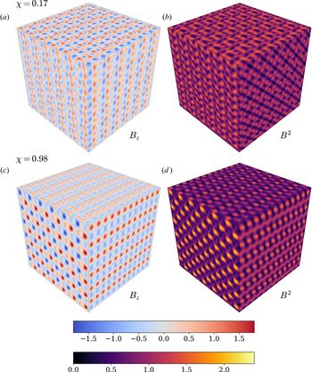
 $\chi =0.98$ are shown in figure 1. Curiously, we have been unable to generate a field with
 $\chi >1$ using this optimisation procedure, which is the condition for the large-scale mode to become unstable in the FOSA (however, see the discussion in § 3.3).
Magnetic-field structure of two force-free equilibria resulting from the numerical optimisation procedure described in § 4.2. The upper colour bar describes the plots of  $B_z$, while the lower colour bar describes the plots of
 $B^2$, in units of
 $\langle v_A^2 \rangle ^{1/2}$ and
 $\langle v_A^2 \rangle$, respectively. Note that the configuration with
 $\chi = 0.17$ has smaller variation in the magnetic-field strength than the configuration with
 $\chi = 0.98$. Indeed, the
 $\chi =0.98$ configuration is hardly ‘tangled’ at all; it more closely resembles a collection of magnetic ‘blobs’ (cf. the discussion in § 3.1).

For each equilibrium configuration, we introduce a sinusoidal velocity shear  $\boldsymbol {u} = 0.05\, \langle v_A^2\rangle ^{1/2}\sin {(2{\rm \pi} x/\lambda )}\hat {\boldsymbol {z}}$, where
 $\lambda =2{\rm \pi} /k_{\rm w}=L$ and
 $\langle v_A^2 \rangle ^{1/2}=\langle B_0^2 \rangle ^{1/2}=\sqrt {3}\,v_E$ is the root-mean-square Alfvén speed, and we measure the evolution of the amplitude of this mode in the Fourier representation of
 $\boldsymbol {u}$.
The three-dimensional, incompressible MHD equations are solved using the DedalusFootnote 8 code (Burns et al. Reference Burns, Vasil, Oishi, Lecoanet and Brown2020) at  $128^3$ resolution (padded for dealiasing according to the 2/3 rule). We take the resistivity
 $\eta = 0$, and thus our simulations are only valid in describing the evolution at early times when the small-scale instability of the equilibrium field configuration has not yet developed and hence the magnetic field structure is still well-resolved.
4.3. Results
4.3.1. Hyperviscous regime
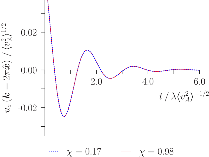
As the simplest ‘control’ case, we first present the results of simulations with hyperviscosity, i.e. with the viscous dissipation term in (2.1) replaced by  $\nu \, \nabla ^6 \boldsymbol {u}$, with the tangled magnetic field at a smaller scale than the hyperviscous cutoff scale. As shown in § 3.1, the small-scale motions cannot develop in this regime, therefore we expect an imposed sinusoidal shear flow to evolve according to (2.7), which might now be called the zeroth-order smoothing approximation (ZOSA) prediction, independently of the small-scale structure of the magnetic field. This is indeed observed, as shown in figure 2, where the evolution of the wave amplitude is plotted for
 $\chi =0.17$ and
 $\chi =0.98$. There is a small relative deviation of
 $\sim 10^{-3}$ between the two curves and the prediction of the ZOSA (2.7) that is not visible on this plot.
Wave amplitude against time for the field configurations with  $\chi =0.17$ and
 $\chi =0.98$ (see figure 1 for the structure of these fields) and using sixth-order hyperviscosity with
 $\nu _6 k_{\rm w}^6=(0.048 \lambda \langle v_A^2 \rangle ^{1/2} ) k_{\rm w}^2$. Despite the difference in the magnetic-field configuration, both fields show an almost identical response to the imposed wave perturbation and evolve according to (2.7), as anticipated by the theory in § 3.1.

4.3.2. Effect of increasing  $\chi$

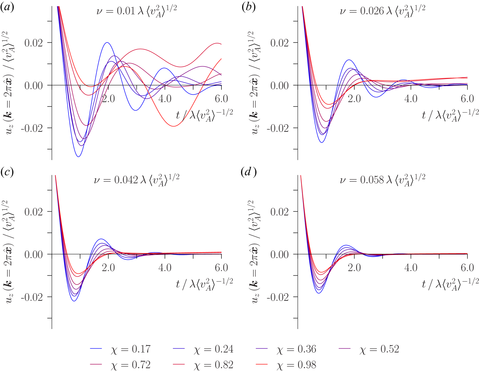
We now turn to the case of Laplacian viscosity. Figure 3 shows the wave evolution for a number of different values of  $\chi$, at a range of Laplacian viscosities. When the viscosity is not very small, the evolution is qualitatively in agreement with the FOSA theory developed in § 3.4, i.e. a larger
 $\chi$ results in a longer wave period and increased damping. At small viscosity, the evolution is dominated by the onset of the instability of the periodic force-free field, which, despite originating at small scales with
 $k\sim k_{\rm t}$, results in a transfer of energy from small to large scales via mergers of magnetic structures (see appendix A.3) that disrupts the waves (this process is not well-resolved in our simulations). We note that the time taken for the instability to develop becomes smaller as
 $\chi$ increases.
Wave amplitude against time for a range of values of  $\chi$, plotted for different viscosities. At large viscosity, fields with larger values of
 $\chi$ support waves with larger period and increased damping, in accordance with § 3.4. At small viscosities, the evolution is dominated by the onset of the instability of the equilibrium field (see appendix A).

4.3.3. Comparison with the analytic theory at different viscosities
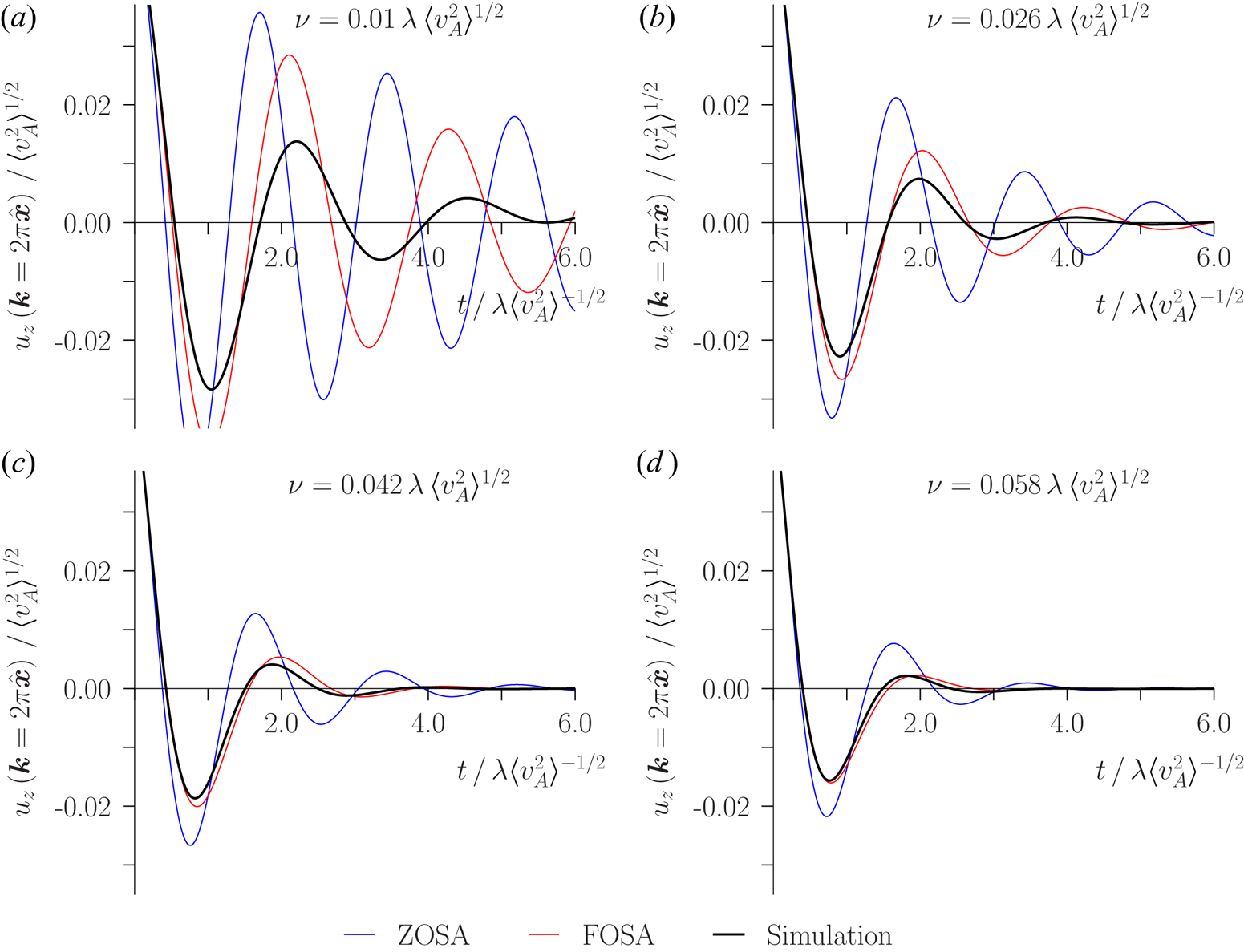
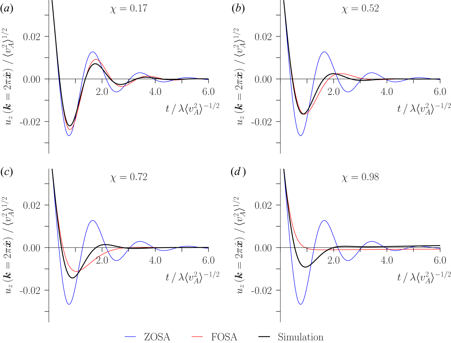
Figure 4 shows the evolution of the wave for  $\chi = 0.51$ and for four different Laplacian viscosities, with the predictions of the ZOSA and FOSA plotted for comparison. We find that the FOSA gives a better prediction in each case, with excellent agreement for large viscosities, correctly capturing the longer wave period and the increased damping observed.


4.3.4. Comparison with the analytic theory at different values of $\chi$

Finally, figure 5 shows the evolution of the wave for different values of  $\chi$ at fixed viscosity,
 $\nu = 0.03 L \langle v_A \rangle ^{1/2}$, with the predictions of the ZOSA and FOSA theories plotted for comparison. Again, we find that the FOSA gives a better prediction in each case, although at large values of
 $\chi$ it fails to predict the numerical result accurately.



4.4. Discussion
Our numerical experiments show that the analytical theory presented in § 3.4 gives a good description of the dynamics of magnetoelastic waves either in the limit of small  $\chi$ or of large viscosity. This is a natural result, as the FOSA assumes greatly simplified small-scale dynamics. Describing the small-scale motions precisely is most important when viscosity is small, because they are less-strongly damped, and when
 $\chi$ is large, because
 $\chi$ encodes the strength of the coupling of large and small scales.
5. Conclusion
In this work, we have studied the large-scale elastic dynamics of MHD equilibrium states with statistically homogeneous and isotropic tangled magnetic-field configurations. We have extended the model presented by Moffatt (Reference Moffatt1986) to consider how the inevitable small-scale inhomogeneity of the magnetic-field structure modifies the dynamics. We have found that in the idealised case of a stable equilibrium state, the frequency of magnetoelastic waves is necessarily reduced as a result of accounting for the inhomogeneity, as a result of relaxation of small-scale structures, which reduces the elastic tension. By employing the FOSA, where couplings between small-scale motions are neglected, we have been able to derive a dispersion relation for magnetoelastic waves in terms of statistical properties of the magnetic-field structure. A key finding is that more intermittent fields are less elastic (see equation 3.25), with the controlling parameter being the variance of the total (thermal + magnetic) pressure. By solving the initial-value problem for a large-scale pulse applied to a viscous fluid, we have further shown that the viscous damping rate of magnetoelastic waves in a magnetic tangle with small-scale inhomogeneity is greater than for a perfectly homogeneous and isotropic Maxwell stress, because the small-scale motions are themselves subject to viscous damping. As we found in § 3.1, these effects are not present in a hyperviscous fluid because dynamically significant motions on the scale of the tangle are prevented.
Interestingly, the frequency reduction owing to intermittency in the magnetic tangle manifests itself in the theory as a reduction in  $\omega ^2$ (see equations 3.14 and 3.23). In principle, this reduction can be arbitrarily large, thereby rendering
 $\omega ^2$ negative. Such a situation would correspond to a field that, by virtue of the coupling of large and small scales, tends to grow large-scale perturbations. It is difficult to intuit such a configuration, which would also be well outside the domain of validity of the FOSA, as discussed in § 3.3. Furthermore, we have not encountered this phenomenon in our numerical study of linear force-free fields, where the field is always elastic to some extent, though can ‘untangle’ via motions on small scales. This said, we do not have a formal proof that such an instability is impossible.
This work is an important first step towards our ultimate goal of understanding the dynamic effect of tangled magnetic field on large-scale motions. In the future, we plan to investigate how the conclusions reached here apply to more general field configurations and to MHD turbulence. The outstanding questions that we hope to address include the following.
(i) How restrictive is the equilibrium assumption? In this work, we have frequently utilised the Hermitian nature of the force operator (see § 3.2), which relies on the unperturbed field being an equilibrium state. While turbulent magnetic fields may be far from equilibrium, simulations of isotropic MHD turbulence have shown an excess of magnetic energy (‘residual energy’) at large scales (Müller & Grappin Reference Müller and Grappin2004, Reference Müller and Grappin2005), hinting that at these scales, the field may organise itself into quasi-equilibrium structures.
(ii) How restrictive is the assumption that the magnetic field has no structure at large scales? In writing (3.1), we assumed that the equilibrium Maxwell stress
$M_0$ had no component at the scale of the magnetoelastic-wave motions. Furthermore, assuming that different large-scale modes are not coupled via their individual coupling to small-scale modes required that positive integer powers of $M_0$ also did not have structure at large scales (see the discussion in § 3.2). These assumptions are justified for synthetic fields of the sort investigated numerically in § 4, but may not be realistic for MHD turbulence (see, for example, Schekochihin et al. Reference Schekochihin, Cowley, Taylor, Maron and McWilliams2004).(iii) What is the effect of magnetic reconnection? In this work, we have exclusively considered flux-frozen magnetic fields. Indeed, as discussed in § 2, the MHD equations cannot be written as closed evolution equations for the Maxwell stress when resistive effects are included. Intuitively, reconnection of magnetic field lines would reduce the magnetic tension that can be maintained at large scales, so we expect reconnecting magnetic fields to be less elastic.


Acknowledgements
It is a pleasure to acknowledge useful conversations with S. J. Benavides and F. Rincon. D.N.H. was supported by an STFC studentship. The work of A.A.S. was supported in part by the UK EPSRC grant EP/R034737/1. S.A.B. was supported in part by STFC grant ST/S000488/1 and the Hintze Family Charitable Foundation. Simulations were performed on the Oxford Hydra cluster.
Editor Roger Blandford thanks the referees for their advice in evaluating this article.
Declaration of interests
The authors report no conflict of interest.
Appendix A. Ideal instability of linear force-free fields
A.1. Existence of an ideal instability
Force-free magnetic fields are an important class of magnetostatic equilibria characterised by a vanishing Lorentz force. Such fields satisfy the equation
 \begin{equation} \boldsymbol{\nabla}\times \boldsymbol{B} = \alpha \boldsymbol{B}, \end{equation}
where  $\alpha (\boldsymbol {r})$ is a scalar function of position, constrained to satisfy
 \begin{equation} \boldsymbol{B}\boldsymbol{\cdot} \boldsymbol{\nabla}\alpha = 0, \end{equation}
by the divergence-free nature of  $\boldsymbol {B}$. Force-free magnetic fields have long enjoyed prominence in plasma astrophysics as a natural relaxed state for magnetically dominated systems. The first such suggestion appears to be by Lüst & Schlüter (Reference Lüst and Schlüter1954), in an effort to explain early investigations that indicated pressure gradients and gravity might be insufficient to balance strong fields in stellar media.
Special significance of linear force-free (LFF) fields, i.e. those for which  $\alpha = \mathrm {constant}$, was first recognised by Chandrasekhar & Woltjer (Reference Chandrasekhar and Woltjer1958), who showed that LFF fields are among the fields that minimise the total Joule heating subject to fixed magnetic energy, and argued on thermodynamic grounds that magnetically dominated systems should relax to this minimum-dissipation state. This argument was refined somewhat by Woltjer (Reference Woltjer1958), who showed that ideal MHD evolution conserves a quantity that later became known as the magnetic helicity,
 \begin{equation} H = \int \mathrm{d}^3 \boldsymbol{r}\,\boldsymbol{A}\boldsymbol{\cdot} \boldsymbol{B}, \end{equation}
and further showed that extremising the magnetic energy subject to the constraint of fixed magnetic helicity produced LFF fields. This extremisation was interpreted as a minimisation of the magnetic energy, and therefore a proof of the stability of LFF equilibria against ideal (helicity-conserving) perturbations. In a later paper, Woltjer (Reference Woltjer1959) argued that this conclusion had been incorrect, because the extremisation process was not guaranteed to produce minima, only extrema. Nonetheless, one state was guaranteed to be stable, the global minimum of the magnetic energy subject to fixed helicity. Substitution of (A 1) into (A 3) gives
 \begin{equation} H = \frac{1}{\alpha}\int \mathrm{d}^3 \boldsymbol{r}\,B^2 = \frac{2E_M}{\alpha}, \end{equation}
and hence the magnetic energy is  $E_M = \alpha H /2$. The force-free state with the smallest magnetic energy for a given magnetic helicity is therefore the one with the smallest value of
 $\alpha$ consistent with the boundary conditions; this state is guaranteed to be stable.Footnote 9
While the question of the stability of states with larger values of  $\alpha$ is not resolved by the extremisation argument, theorems have been proposed regarding the stability of such states. These theorems mostly rely on the energy principle of Bernstein et al. (Reference Bernstein, Frieman, Kruskal and Kulsrud1958), which states that an MHD equilibrium state is stable if the second-order change in the total energy
 \begin{equation} \delta W_2 = \tfrac{1}{2} \int \mathrm{d}^3 \boldsymbol{r} \left[\left(\boldsymbol{\xi}\boldsymbol{\cdot}\boldsymbol{\nabla}p_0\right)\boldsymbol{\nabla}\boldsymbol{\cdot}\boldsymbol{\xi}+\gamma p_0 \left(\boldsymbol{\nabla}\boldsymbol{\cdot}\boldsymbol{\xi}\right)^2 + \left(\boldsymbol{\nabla}\times\boldsymbol{B}_0\right)\boldsymbol{\cdot}\left(\boldsymbol{\xi}\times\delta\boldsymbol{B}\right)+\left|\delta \boldsymbol{B}\right|^2\right] \end{equation}
is positive for any displacement field  $\boldsymbol {\xi }$, where
 $\gamma$ is the adiabatic index,
 $p$ is the thermal pressure, the subscript zero refers to equilibrium quantities, and
 $\delta \boldsymbol {B} = \boldsymbol {\nabla }\times (\boldsymbol {\xi } \times \boldsymbol {B}_0)$. The first term is zero for a force-free equilibrium, while the second is positive definite, but can always be made small by taking
 $p_0 \rightarrow 0$. Hence, the only terms relevant to the stability of force-free fields are the final two. Substituting the force-free condition, (A 1), into (A 5), we obtain
 \begin{equation} \delta W_2 = \tfrac{1}{2} \int \mathrm{d}^3 \boldsymbol{r} \left[\left(\boldsymbol{\nabla}\times\delta\boldsymbol{ \boldsymbol{A}}\right)^2-\alpha\, \delta \boldsymbol{A}\boldsymbol{\cdot} \left(\boldsymbol{\nabla}\times\delta\boldsymbol{A}\right) \right], \end{equation}
where  $\delta \boldsymbol {A} = \boldsymbol {\xi }\times \boldsymbol {B_0}$. From this or equivalent expressions, it has been shown that more-or-less restricted classes of perturbations will give
 $\delta W_2>0$ for more-or-less restricted classes of LFF fields, and hence those equilibria are stable to such perturbations.Footnote 10 Classes of perturbations to which LFF fields have been shown to be stable (for any constant
 $\alpha$) include: radial expansions; displacements along one spatial direction (i.e.
 $\boldsymbol {\xi }=\xi ( \boldsymbol {r})\boldsymbol {n}$, where
 $\xi (\boldsymbol {r})$ is an arbitrary scalar function of position and
 $\boldsymbol {n}$ is a constant vector); axisymmetric perturbations (of axisymmetric LFF fields only); and perturbations that vanish outside of a region with spatial extent
 $d<1/|\alpha |$ (Woltjer Reference Woltjer1958; Molodensky Reference Molodensky1974). To each of these perturbations it is possible to add any component along
 $\boldsymbol {B}_0$, because this does not change
 $\delta \boldsymbol {A}$.
Voslamber & Callebaut (Reference Voslamber and Callebaut1962), however, showed by means of a counterexample that not all LFF fields are stable; they found that there exist axisymmetric field configurations that are unstable to a class of non-axisymmetric perturbations. This dashed the hopes of proving a general stability theorem for LFF fields until the problem was revisited by Moffatt (Reference Moffatt1986), who showed by expanding  $\boldsymbol {B}_0$ and
 $\boldsymbol {\xi }$ in Fourier modes that arbitrary periodic LFF equilibria are stable to arbitrary periodic perturbations. Indeed, the stability of LFF fields was the motivation for the consideration of the magnetoelastic wave problem by Moffatt (Reference Moffatt1986). Despite the apparent conflict between the result of Voslamber & Callebaut (Reference Voslamber and Callebaut1962) and Moffatt's stability theorem, it was not until much more recently that a counterexample was explicitly presented by Er-Riani et al. (Reference Er-Riani, Naji and El Jarroudi2014), who showed that there exist periodic force-free fields that are unstable to ideal periodic perturbations, as long as these perturbations are allowed to have wavevectors smaller than
 $\alpha$.Footnote 11 Soon after, East et al. (Reference East, Zrake, Yuan and Blandford2015) were able to find energy-decreasing perturbations for a number of LFF fields by numerical minimisation of (A 5) under variation of the Fourier coefficients in the expansion of
 $\boldsymbol {\xi }$. Indeed, they reported that they were able to find energy-decreasing perturbations for every LFF field that they considered, when Fourier modes with wavenumbers smaller than
 $\alpha$ were allowed. We too have encountered instability in each of the fields that we have investigated numerically in this work.
We note that there do exist stable periodic LFF fields, though only in the restricted case of no magnetic curvature. An example is the field  $\boldsymbol {B} = B_0 (0,\sin \alpha x,\cos \alpha x)$ which represents a uniform magnetic field in any plane of constant
 $x$, with direction rotating as
 $x$ is varied. The stability of this configuration against a restricted class of periodic perturbations was demonstrated by Vekshtein (Reference Vekshtein1989); here, we note that for a general periodic perturbation
 $\boldsymbol {\xi }(\boldsymbol {r})=(\xi _x(\boldsymbol {r}), \xi _y(\boldsymbol {r}), \xi _z(\boldsymbol {r}))^{\mathrm {T}}$ it is possible to show via an elementary (though somewhat tedious) calculation that
 \begin{align} \delta W_2 &= \frac{1}{2} B_0^2 \int \mathrm{d}^3 \boldsymbol{r} \left[\left(\cos\alpha x \,\frac{\partial \xi_x}{\partial x}+\cos\alpha x \,\frac{\partial \xi_y}{\partial y}-\sin\alpha x \,\frac{\partial \xi_z}{\partial y} \right)^2 \right.\nonumber\\ & \quad \left.+\left(\sin\alpha x \,\frac{\partial \xi_x}{\partial x}+\sin\alpha x \,\frac{\partial \xi_z}{\partial z}-\cos\alpha x \,\frac{\partial \xi_y}{\partial z} \right)^2+ \left(\sin\alpha x \,\frac{\partial \xi_x}{\partial y}+\cos\alpha x \,\frac{\partial \xi_x}{\partial z} \right)^2\right]. \end{align}
The integrand is manifestly positive definite, so this configuration is stable to ideal perturbations, for any  $\alpha$.Footnote 12
Whether there exist any periodic LFF configurations with magnetic curvature that are stable to arbitrary perturbations is, at present, unknown, as there have been no general theorems of instability (see Zrake & East (Reference Zrake and East2016) for speculations that stable structures may exist in the nonlinear force-free case). The existence of stable force-free configurations would be highly significant for astrophysical systems where magnetic-field structures are smaller than the system size, such as the hot, rarefied plasma between galaxies in clusters.
A.2. Physical nature of the instability
Since its (re)discovery in 2014, the instability of LFF fields has attracted attention as a means of studying particle acceleration by magnetic reconnectionFootnote 13 (Nalewajko et al. Reference Nalewajko, Zrake, Yuan, East and Blandford2016; Lyutikov et al. Reference Lyutikov, Sironi, Komissarov and Porth2017) in a more realistic setting than the typical Harris-type current sheet configuration.
Lyutikov et al. (Reference Lyutikov, Sironi, Komissarov and Porth2017) have proposed a mechanism for the instability of two-dimensional LFF fields, by arguing that these fields describe a regular array (in the  $xy$-plane) of alternating currents (directed along
 $z$). Since like currents attract, this configuration is unstable, with similarly directed currents ultimately merging.
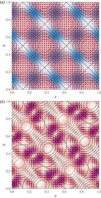
In this work, we have been primarily motivated by the manifestation of the Lorentz force as a local magnetic tension in incompressible MHD. It is therefore instructive to see how the instability arises in this picture. Figure 6 shows the ideal instability of the two-dimensional LFF given by
 \begin{equation} \boldsymbol{B}=B_0 \left(-\sin4{\rm \pi} y, \cos 4{\rm \pi} x, \cos4{\rm \pi} y - \sin 4 {\rm \pi} x \right), \end{equation}
which has  $\alpha = 4{\rm \pi}$. Since the field is translationally invariant in
 $z$, only its component in the
 $xy$-plane contributes to the magnetic tension. An unstable perturbation can be obtained by trialling a truncated Fourier series in (A 5); evaluation of the integral gives a quadratic form in the coefficients of the Fourier modes, which can be diagonalised and the perturbation that minimises
 $\delta W$ obtained (up to an arbitrary normalisation constant). By carrying out this procedure, we find that
 \begin{align} \xi_x &= 7.34754 \cos (2{\rm \pi} x+2 {\rm \pi} y)-7.34754 \sin (2 {\rm \pi} x+2 {\rm \pi} y) + 1.30549 \cos (2 {\rm \pi} x-6 {\rm \pi} y)\nonumber\\ &\quad -1.30549 \sin (2 {\rm \pi} x-6 {\rm \pi} y)+0.447807 \cos (6 {\rm \pi} x-2 {\rm \pi} y)\nonumber\\ &\quad +0.447807 \sin (6 {\rm \pi} x-2 {\rm \pi} y) + \sin (6 {\rm \pi} x+6 {\rm \pi} y)+\cos (6 {\rm \pi} x+6{\rm \pi} y), \end{align}
 \begin{align} \xi_y &= -7.34754 \cos (2 {\rm \pi} x+2 {\rm \pi} y)+7.34754 \sin (2 {\rm \pi} x+2 {\rm \pi} y) + 0.435165 \cos (2 {\rm \pi} x-6 {\rm \pi} y) \nonumber\\ &\quad - 0.435165 \sin (2 {\rm \pi} x-6 {\rm \pi} y)+1.34342 \cos (6 {\rm \pi} x-2 {\rm \pi} y)\nonumber\\ &\quad + 1.34342 \sin (6 {\rm \pi} x-2 {\rm \pi} y) - \sin (6 {\rm \pi} x+6 {\rm \pi} y)- \cos (6 {\rm \pi} x+6 {\rm \pi} y), \end{align}
gives  $\delta W_2<0$. This perturbation (with convenient normalisation) is shown in figure 6, together with the perturbed magnetic-field structure. We observe that the perturbation represents a non-trivial deformation of the magnetic field structure that mostly consists of the ‘magnetic cells’ that make up the field configuration sliding past each other in layers, with smaller perturbations to the field at the boundaries of each cell that generate a magnetic tension force whose net direction is along the direction of the displacement of the layer, preventing the configuration from returning to its original state.
 $(a)$ Black lines are level lines of
 $B_z$ for the field defined by (A 8). By the LFF condition and
 $z$-independent nature of the field, these are also the field lines of the dynamically important
 $xy$-plane field. Solid black lines have
 $B_z>0$, so the in-plane field has anticlockwise circulation, while dashed black lines have
 $B_z<0$, so the in-plane field has clockwise circulation. The strength of the in-plane field is shown in blue. Red arrows show a perturbation for which
 $\delta W <0$.
 $(b)$ The field configuration obtained by applying this perturbation. Black lines again show the
 $xy$-plane field, while blue arrows show the non-compressive part of the magnetic tension force, with the size of this force shown in red.

The timescale for the development of instability can be estimated analytically using energy conservation for the truncated system:
 \begin{equation} \frac{{\textrm{d}}}{{\textrm{d}} t}\left(\frac{1}{2}\int {\textrm{d}}^3\boldsymbol{r}\,\dot{\xi}^2 + \delta W\right) = -\nu\int {\textrm{d}}^3\boldsymbol{r}|\boldsymbol{\nabla} \boldsymbol{\xi}|^2. \end{equation}
When the fluid is inviscid, the timescale can be estimated by balancing the kinetic and potential energy terms and solving the resulting eigenvalue problem for the growth rate of the unstable mode. For a viscously dominated fluid, the rate of change of potential energy is balanced with the rate of energy dissipation by viscosity.
Solving the eigenvalue problem for the truncated system, we find growth rates of  $0.0930196\,\alpha B_0$ for the inviscid case and
 $0.0135899\, B_0^2/\nu$ for the viscous case. The dimensional form of these results is inevitable, but the numerical prefactors turn out to be small, particularly in the viscous case, indicating that the growth rate of the instability should be slower than a naïve estimate of the kind made in § 4.1 would indicate. The reason for this is apparent from figure 6, which shows that force responsible for driving the relative motions of the layers of magnetic cells is mostly generated by the perturbations to the field at the boundary of each cell, and the component of this force along the direction of motion of the layer is small. The viscous growth rate is further suppressed by the fact that the perturbations at the boundaries of each cell that are responsible for generating forces are at a smaller scale than the cell size, and hence are damped more strongly by viscosity.
Similar considerations may apply to the more complicated three-dimensional ‘tangled’ equilibria that we have considered in the main text, explaining why the small-scale instability develops slowly in our simulations. Lyutikov et al. (Reference Lyutikov, Sironi, Komissarov and Porth2017) have also argued that three-dimensional magnetic configurations should be more stable than two-dimensional ones because the field cannot be naturally decomposed into sliding layers.
A.3. Nonlinear evolution
The nonlinear evolution of the instability has been extensively studied using both force-free electrodynamics (FFE) simulations (East et al. Reference East, Zrake, Yuan and Blandford2015; Zrake & East Reference Zrake and East2016; Lyutikov et al. Reference Lyutikov, Sironi, Komissarov and Porth2017) and kinetic simulations (Nalewajko et al. Reference Nalewajko, Zrake, Yuan, East and Blandford2016; Yuan et al. Reference Yuan, Nalewajko, Zrake, East and Blandford2016; Lyutikov et al. Reference Lyutikov, Sironi, Komissarov and Porth2017; Nalewajko Reference Nalewajko2018) of simple LFF configurations, the so-called Arnold–Beltrami–Childress (ABC) fields, of which (A 8) is an example.
In these studies, the late-time evolution is characterised by an ‘untangling’ and merging of magnetic flux tubes, with an associated transfer of magnetic energy from small to large scales. Indeed, Blandford et al. (Reference Blandford, Yuan, Hoshino and Sironi2017) suggested that the particle acceleration that occurs during such an untangling may power dramatic flares in high-energy astrophysical sources. The ultimate state of the system is the stable LFF state with the smallest  $\alpha$ compatible with the size of the box, in accordance with J.B. Taylor relaxation (see appendix A.1). Interestingly, in two dimensions, Zrake & East (Reference Zrake and East2016) have found with force-free electrodynamics simulations that the system does not relax to an LFF state, but instead to a configuration of nonlinear force-free magnetic ‘bubbles’, which they argue is a consequence of the existence in two dimensions of invariants additional to magnetic helicity. East et al. (Reference East, Zrake, Yuan and Blandford2015) found indications that it is possible for the nonlinear system to evolve into a transient LFF state with
 $\alpha$ larger than the smallest value permitted by the geometry, though this does not appear to have been reproduced in later studies.
Appendix B. Proof that the amplitudes of fast Laplace modes of the large-scale motion vanish as $\epsilon \rightarrow 0$

In this appendix, we show that the Laplace amplitudes of any fast motion on large scales vanishes compared with the amplitude of slow motions, as  $\epsilon \rightarrow 0$. This justifies the neglect of
 $p^2$ in the denominator of the coupling term in (3.28).
Retaining  $p^2$ in (3.28), the dispersion relation (3.31) becomes
 \begin{equation} D(p_n) \equiv p_n^2+v_E^2k^2-\sum_{\boldsymbol{k}'}\frac{A_{zj}(\boldsymbol{k}_{\rm w}, \boldsymbol{k}') A_{jz}(\boldsymbol{k}', \boldsymbol{k}_{\rm w})}{p_n^2+k'^2 v_E^2 + \nu k'^2 p_n} +\nu k^2 p_n = 0. \end{equation}
Using the non-dimensionalisation  $\hat {\nu }=\nu k_{\rm w}/v_E$,
 $\hat {p}=p/k_{\rm w} v_E$, we can write (B 1) as
 \begin{equation} \hat{p}^2+1-\sum_{\boldsymbol{k}'} \frac{A_{zj}(\boldsymbol{k}_{\rm w}, \boldsymbol{k}') A_{jz}(\boldsymbol{k}', \boldsymbol{k}_{\rm w})/k'^2}{\epsilon_{k'}^2\hat{p}^2 +1 + \hat{\nu} \hat{p}}+\hat{\nu}\hat{p} = 0, \end{equation}
where  $\epsilon _{k'}=k/k'\sim \epsilon$, and, as before,
 $\epsilon \sim k_{\rm w}/k_{\rm t} \ll 1$. This equation has
 $2W+2$ solutions, where
 $W$ is the number of distinct wavenumbers among the small-scale modes to which the large-scale perturbation couples – this corresponds to the number of distinct small-scale frequencies that are possible.Footnote 14 To evaluate the Laplace amplitude according to (3.30), it is helpful to factorise the dispersion relation. Factoring out
 $1/(p^2+1/\epsilon _{k'}^2+\hat {\nu }\hat {p}/\epsilon _{k'}^2)$ for each of the
 $W$ terms in the sum in (B 2) leaves a polynomial whose leading coefficient is
 $1$, and whose roots are all the solutions of (B 2): this polynomial can be factorised as
 $\prod _{m}(\hat {p}-\hat {p}_{m})$, i.e.
 \begin{equation} \hat{p}^2+1-\sum_{\boldsymbol{k}'} \frac{A_{zj}(\boldsymbol{k}_{\rm w}, \boldsymbol{k}') A_{jz}(\boldsymbol{k}', \boldsymbol{k}_{\rm w})/k'^2}{\epsilon_{k'}^2\hat{p}^2 +1 + \hat{\nu} \hat{p}}+\hat{\nu}\hat{p}=\prod_{k'}\frac{1}{p^2+1/\epsilon_{k'}^2+\hat{\nu}\hat{p}/\epsilon_{k'}^2} \prod_{m=1}^{2W+2}\left(p-p_m\right), \end{equation}
where the first product is over the  $W$ distinct values of
 $k'=|\boldsymbol {k}'|$.
According to (3.30), the Laplace amplitudes are computed according to
 \begin{align} A_n& = \text{Res} \left[ \frac{p}{D(p )} , p\rightarrow p_n \right]\nonumber\\ &=\lim_{\hat{p}\rightarrow \hat{p}_n}\frac{\displaystyle\hat{p}\left(\hat{p}-\hat{p}_n\right)\prod_{k'}\left(\hat{p}^2+1/\epsilon_{k'}^2+\hat{\nu}\hat{p}/\epsilon_{k'}^2\right)}{\displaystyle\prod_{m=1}^{2W+2}\left(\hat{p}-\hat{p}_m\right)} \nonumber\\ & = \frac{\displaystyle\hat{p}_n\prod_{k'}\left(\hat{p}^2+1/\epsilon_{k'}^2+\hat{\nu}\hat{p}/\epsilon_{k'}^2\right)}{\displaystyle\prod_{m=1,m\neq n}^{2W+2}\left(\hat{p}_n-\hat{p}_m\right)}. \end{align}
The scaling of  $A_n$ with
 $\epsilon$ will depend on the ordering of
 $\hat {\nu }$ with respect to
 $\epsilon$ – this determines whether or not the small-scale magnetic field is viscously dominated. Generally, we can write
 $\hat {\nu }=O(\epsilon ^{\beta })$ and consider the scaling of
 $A_n$ for different values of
 $\beta$.
If  $\beta \geq 1$, the small-scale field is not overdamped by viscosity. Any solution for which
 $\epsilon _{k'}^2\hat {p}^2$ is not negligible in the denominator of (B 2) is a balance of
 $\epsilon _{k'}^2\hat {p}^2$ and
 $1$ (and
 $\hat {\nu }\hat {p}$, if
 $\beta =1$), so
 $p\sim \epsilon ^{-1}$. We then have
 \begin{equation} \prod_{m\neq n}\left(p_n-p_m\right) \sim \epsilon^{-(2W+1)}. \end{equation}
Each term in the product  $\prod _{k'}(p^2+1/\epsilon _{k'}^2+\hat {\nu }\hat {p}/\epsilon _{k'}^2)$ is
 $\sim 1/\epsilon ^2$ apart from one, which is that for which
 $p_n$ is an approximate root. The leading-order scaling of this term will be
 $\epsilon ^2$, in order to balance the other terms in (B 2), therefore,
 \begin{equation} \prod_{k'}\left(p^2+1/\epsilon_{k'}^2+\hat{\nu}\hat{p}/\epsilon_{k'}^2\right)\sim \epsilon^{-2(W-1)}\epsilon^2=\epsilon^{4-2W}. \end{equation}
With these scalings, (B 4) gives  $A_n\sim \epsilon ^4$.
Alternatively, if  $\beta <1$, the small-scale field is strongly damped by viscosity. We argue similarly to before: any solution for which
 $\epsilon _{k'}^2\hat {p}^2$ is not negligible in the denominator of (B 2) is a balance of
 $\epsilon _{k'}^2\hat {p}^2$ and
 $\hat {\nu }\hat {p}$, so
 $p\sim \epsilon ^{\beta -2}$. We then have
 \begin{equation} \prod_{m\neq n}\left(p_n-p_m\right) \sim \left(\epsilon^{\beta-2} \right) ^{2W+1}, \end{equation}
while
 \begin{equation} \prod_{k'}\left(p^2+1/\epsilon_{k'}^2+\hat{\nu}\hat{p}/\epsilon_{k'}^2\right)\sim \left(\epsilon^{2\beta-4} \right)^{W-1}\epsilon^{4-2\beta}\sim\left(\epsilon^{\beta-2}\right)^{2W-4}. \end{equation}
With these scalings, (B 4) gives  $A_n\sim \epsilon ^{8-4\beta }$.
In both cases,  $A_n\rightarrow 0$ as
 $\epsilon \rightarrow 0$.