1 Introduction
The scattering of vortical and entropic waves by a cascade of blades is of considerable importance in aeroengine design. It is known that a large component of the noise generated by a modern high-bypass ratio turbofan system is due to the interaction of unsteady wakes generated by the upstream rotors interacting with downstream stators in so-called ‘rotor–stator interaction’ (Peake & Parry Reference Peake and Parry2012). In order to meet increasingly strict restrictions on aircraft noise, coupled with expected growth in air traffic, enhanced modelling and physical understanding of the complex aeroacoustic and aerodynamic interactions involved in rotor–stator interaction are required.
The noise produced by rotor–stator interaction is well understood for stators modelled as flat plates at zero angle of attack (Koch Reference Koch1971; Peake Reference Peake1992, Reference Peake1993; Peake & Kerschen Reference Peake and Kerschen1995; Glegg Reference Glegg1999; Posson, Roger & Moreau Reference Posson, Roger and Moreau2010). However, these models do not take into account the realistic and important effects of mean flow gradients refracting both the incident gust and scattered field. Surprisingly, the corresponding analysis for realistic aerofoil geometry (including both camber and thickness) have not been investigated to the same extent, despite knowledge that realistic geometries can have significant effects on the upstream acoustic field (Peake & Kerschen Reference Peake and Kerschen1997; Evers & Peake Reference Evers and Peake2002; Peake & Kerschen Reference Peake and Kerschen2004). In each of these approaches, the flow is calculated by splitting the domain into inner regions around each leading edge, and matching with an outer solution. This approach is necessary due to the large gradients which occur at the leading edge, but cannot reproduce the details of the flow field in the crucial inter-blade region, particularly the unsteady surface pressure.
Numerical simulations of the noise produced in rotor–stator interaction using computational aeroacoustics (CAA) codes (Verdon Reference Verdon1993; Hixon, Sescu & Allampalli Reference Hixon, Sescu and Allampalli2010; Gea-Aguilera et al. Reference Gea-Aguilera, Gill, Zhang and Nodé-Langlois2016; Grace Reference Grace2016) can typically provide details of the unsteady field throughout the whole flow domain, but these methods can be computationally costly. An analytical expression is useful in elucidating the role of various parameters without the need for expensive computations. The present research is focused on extending the analysis of Glegg (Reference Glegg1999) and Posson et al. (Reference Posson, Roger and Moreau2010), which only considered the influence of flat plates at zero angle of attack. In the former, Glegg found an analytical solution for the acoustic field outside of the flat-plate blade row, and Posson et al. (Reference Posson, Roger and Moreau2010) extended this to be able to calculate the unsteady field within the inter-blade region. Our new analytic solution, which is valid throughout the entire flow domain, extends these two works further and can be used to swiftly calculate the effects of small geometry on the far-field acoustics and unsteady blade loading, as well as providing a benchmark to test CAA simulations against.
The model in the present work is subject to some asymptotic restrictions. Firstly, the aerofoils are assumed to be formally ‘thin’, so that background flow gradients are  $O(\unicode[STIX]{x1D716})$ perturbations from uniformity. Secondly, the frequency must satisfy
 $k\unicode[STIX]{x1D716}\ll 1$, where
 $k$ is the reduced frequency. Far from being restrictive, this asymptotic regime crucially accounts for the first few blade passing frequencies (BPFs), which significantly contribute to engine noise. Typically, the upstream rotors move and shed wakes which impinge on the cascade at the blade passing frequency; accurate modelling of the scattering of incident wakes of frequencies close to the BPFs is essential because they usually occur in the most sensitive frequency regime of human hearing (Dittmar Reference Dittmar1972). Additionally, the BPFs occur at large sound pressure levels, so they are usually the loudest tones, as well as the most annoying. Presently, other analytic cascade interaction models that account for aerofoil geometry (Peake & Kerschen Reference Peake and Kerschen1997, Reference Peake and Kerschen2004; Evers & Peake Reference Evers and Peake2002) are restricted to high frequencies that cannot account for these critical interactions.
In § 2 we discuss the modelling assumptions and give some key details of the form of the background mean flow, which prove useful in later analysis. In § 2.2 the governing equations for the acoustic potential function are derived using rapid distortion theory, as in Goldstein (Reference Goldstein1978), and the corresponding boundary conditions are derived. A perturbation expansion is used, where the small parameter  $\unicode[STIX]{x1D716}$ is the order of magnitude of the distortion of the mean flow from uniform flow. This expansion yields two equations: one at
 $O(1)$ and another at
 $O(\unicode[STIX]{x1D716})$. The leading order,
 $O(1)$, equation is the flat-plate problem solved previously by Glegg (Reference Glegg1999). In § 3.2, we solve the
 $O(\unicode[STIX]{x1D716})$ equation for the Fourier transform of the jump in potential either side of the blade. Whilst more complicated than the
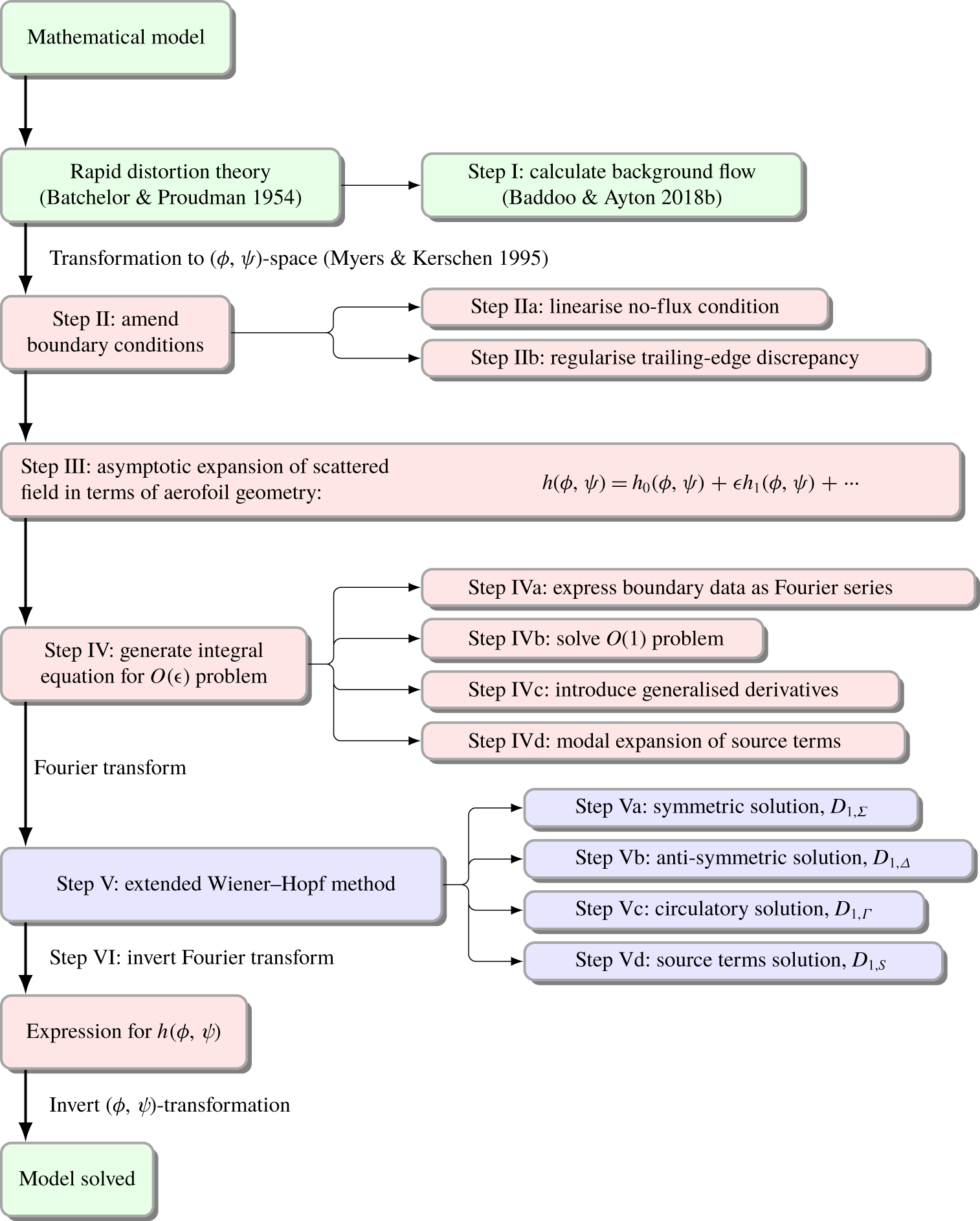
 $O(1)$ problem due to forcing terms arising from the mean flow distortion, this problem can be solved using a similar approach to that of Glegg (Reference Glegg1999). In § 4 this Fourier transform is inverted, using a similar method to Posson et al. (Reference Posson, Roger and Moreau2010). In § 5 various aeroacoustic results are discussed. Finally, in § 6, we summarise our work and suggest future directions of research. We illustrate the important details of the procedure in a road map in figure 1.
Schematic diagram illustrating the solution method of the present paper. The colour of each box represents the space in which the relevant analysis takes place: green denotes physical  $(x,y,z)$-space; red, parametric
 $(\unicode[STIX]{x1D719},\unicode[STIX]{x1D713},z)$-space; and blue, spectral
 $\unicode[STIX]{x1D6FE}$-space.

2 Modelling
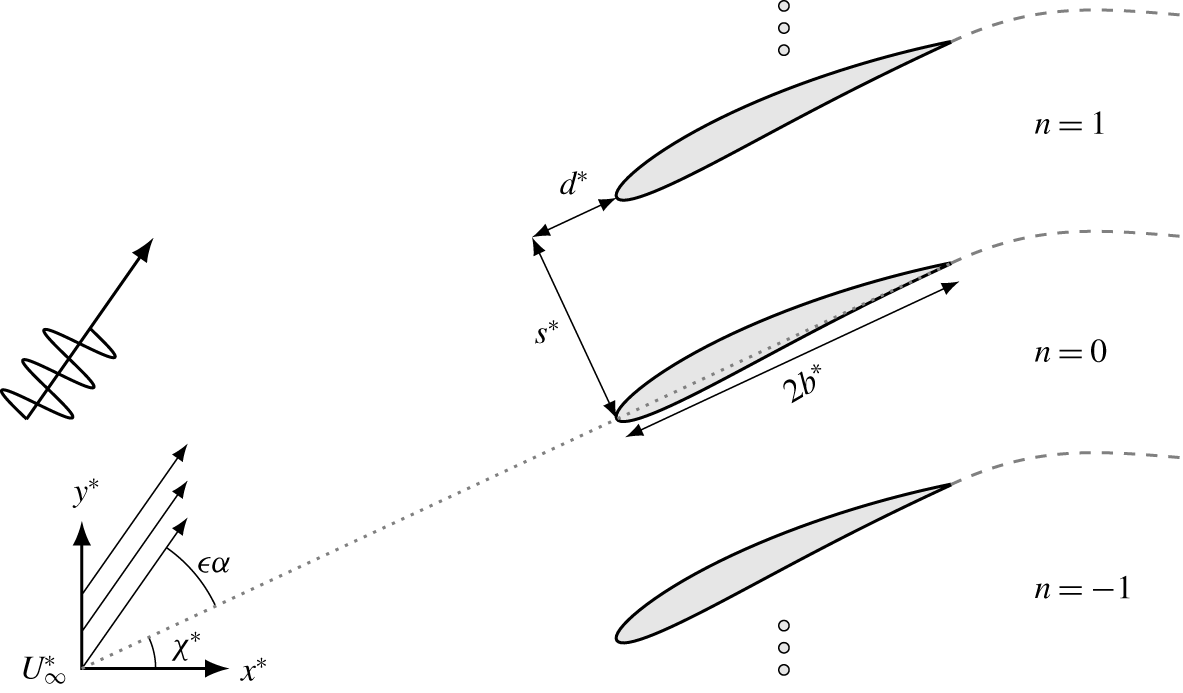
We consider a linear cascade of blades in a subsonic flow as illustrated in figure 2. The blades are separated by  $d^{\ast }$ in the chordwise direction,
 $s^{\ast }$ in the normal direction and have infinite span in the
 $x_{3}^{\ast }$ direction. (Here
 $\ast$ denotes a dimensional quantity.) The aerofoils have semi-chord length
 $b^{\ast }$ in Cartesian coordinates
 $(x^{\ast },y^{\ast })$ and the coordinate origin is taken to be at the leading edge of the 0th blade. We non-dimensionalise lengths by
 $b^{\ast }$. We assume that the blades have non-trivial geometry, such that the upper and lower surfaces of the blade,
 $\unicode[STIX]{x1D716}y_{s\pm }$, can be described by
 $$\begin{eqnarray}\unicode[STIX]{x1D716}y_{s\pm }(x)=\pm \unicode[STIX]{x1D716}y_{th}(x)+\unicode[STIX]{x1D716}y_{c}(x),\end{eqnarray}$$
where the subscripts  $c$ and
 $th$ denote camber and thickness respectively and
 $\unicode[STIX]{x1D716}\ll 1$. We restrict our analysis to bodies that have, at worst, parabolic noses, i.e.
 $y_{th}\sim \unicode[STIX]{x1D716}th^{\prime }\sqrt{x}$ as
 $x\rightarrow 0^{+}$ where
 $th=\unicode[STIX]{x1D716}th^{\prime }$ is the maximum thickness of the aerofoil, which is common in analytical aerofoil interaction problems (Tsai Reference Tsai1992; Ayton & Peake Reference Ayton and Peake2013). Additionally, we require that the derivative of camber is bounded and continuous. The steady mean flow far upstream is uniform with speed
 $U_{\infty }^{\ast }$ (which we will use to non-dimensionalise velocities). We also permit the upstream mean flow at infinity to be at a small angle of attack,
 $\unicode[STIX]{x1D716}\unicode[STIX]{x1D6FC}$.
A cascade of realistic aerofoils at stagger angle  $\unicode[STIX]{x1D712}^{\ast }$ and incidence angle
 $\unicode[STIX]{x1D716}\unicode[STIX]{x1D6FC}$ subject to a convected disturbance. The dotted line indicates the chordwise direction and the dashed lines represent the unsteady wakes.

We denote the velocity potential and streamfunction of the steady background flow through the cascade as  $\unicode[STIX]{x1D719}^{\ast }$ and
 $\unicode[STIX]{x1D713}^{\ast }$ respectively, which we non-dimensionalise as
 $$\begin{eqnarray}\unicode[STIX]{x1D719}=\frac{\unicode[STIX]{x1D719}^{\ast }}{U_{\infty }^{\ast }b^{\ast }},\quad \unicode[STIX]{x1D713}=\unicode[STIX]{x1D6FD}_{\infty }\frac{\unicode[STIX]{x1D713}^{\ast }}{U_{\infty }^{\ast }b^{\ast }},\quad x_{3}=\frac{x_{3}^{\ast }}{b^{\ast }},\end{eqnarray}$$
where  $\unicode[STIX]{x1D6FD}_{\infty }=\sqrt{1-M_{\infty }^{2}}$ is the Prandtl–Glauert factor and
 $M_{\infty }$ is the mean flow Mach number far upstream. The density is non-dimensionalised with respect to the density far upstream
 $\unicode[STIX]{x1D70C}^{\ast }$ and the pressure is non-dimensionalised with respect to
 $\unicode[STIX]{x1D70C}^{\ast }{U_{\infty }^{\ast }}^{2}$.
2.1 Steady flow
Before we can approach the unsteady aeroacoustics, we must first solve the steady background flow. This is step I in the road map (figure 1). There are several ways to calculate the potential flow through a cascade of aerofoils. By utilising a conformal map from a canonical circular domain to a cascade of flat plates, the flow for an arbitrary incident angle can be calculated analytically (Robinson & Laurmann Reference Robinson and Laurmann1956). Whilst this solution is exact, the expression for the conformal mapping is not invertible and the flow may only be written implicitly. Another method that is ubiquitous in thin-aerofoil theory is the method of singularities: the rigid aerofoil surface may be modelled as a distribution of mass sources and vortices on the chord (for thin aerofoils) or the surface (for thick aerofoils). This theory has previously been applied to cascades (Falcão Reference Falcão1975; Schulten Reference Schulten1982). The vortex distribution is typically written as a Glauert sine series or, equivalently, a series of weighted Chebyshev polynomials. These methods have been combined by Evers & Peake (Reference Evers and Peake2002) to provide an analytical expression for the steady flow near the leading edges.
Recently, exact solutions for the flow around thin, slightly staggered aerofoils have been found by modelling the flow as a Riemann–Hilbert problem (Baddoo & Ayton Reference Baddoo and Ayton2018b). The resulting expression is a clear extension of the classical thin-aerofoil theory for a single blade (Thwaites Reference Thwaites1960) and is invertible: given a particular tangential surface velocity, the corresponding aerofoil geometry can be found. However, we want to take into account large stagger angles, so a different approach is required here, although this analytical result will be useful to benchmark any other solutions.
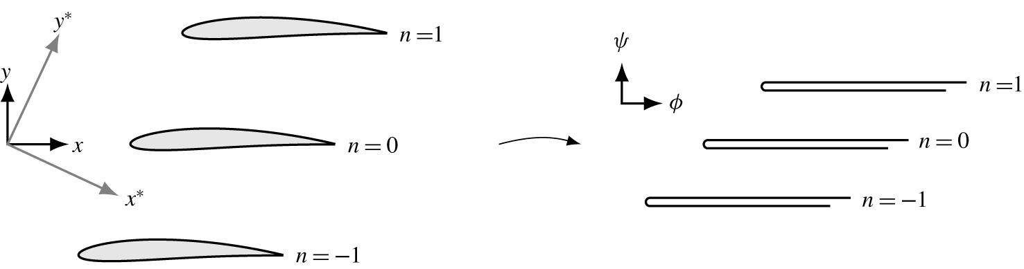
To aid application of the boundary conditions in the unsteady problem, we will transform from non-dimensional Cartesian coordinates  $(x,y)$ to potential-streamline coordinates
 $(\unicode[STIX]{x1D719},\unicode[STIX]{x1D713})$ as is typical for realistic-geometry aerofoil interactions studied analytically (Myers & Kerschen Reference Myers and Kerschen1995, Reference Myers and Kerschen1997; Peake & Kerschen Reference Peake and Kerschen1997, Reference Peake and Kerschen2004; Ayton & Peake Reference Ayton and Peake2013; Ayton Reference Ayton2017). The relationship between coordinates is given by
 $$\begin{eqnarray}z_{\unicode[STIX]{x1D6FD}}=z_{\unicode[STIX]{x1D719}}+\unicode[STIX]{x1D716}F(z_{\unicode[STIX]{x1D719}}),\end{eqnarray}$$
where  $z_{\unicode[STIX]{x1D6FD}}=x+\text{i}\unicode[STIX]{x1D6FD}_{\infty }y$ are the non-dimensional coordinates in the Prandtl–Glauert space (where the flow is incompressible) and
 $z_{\unicode[STIX]{x1D719}}=\unicode[STIX]{x1D719}+\text{i}\unicode[STIX]{x1D713}$. The coordinate transformation is illustrated in figure 3.
 $F(z_{\unicode[STIX]{x1D719}})$ is the complex potential of the steady flow written as
 $q(z_{\unicode[STIX]{x1D719}})-\text{i}\unicode[STIX]{x1D707}(z_{\unicode[STIX]{x1D719}})=F^{\prime }(z_{\unicode[STIX]{x1D719}})$ where the amplitude of the steady flow is given by
 $1+\unicode[STIX]{x1D716}q$, in the direction making an angle
 $\unicode[STIX]{x1D716}\unicode[STIX]{x1D707}$ with the horizontal. Consequently, we may write the non-dimensional perturbation to horizontal uniform flow as (Baddoo & Ayton Reference Baddoo and Ayton2018b)
 $$\begin{eqnarray}q(z_{\unicode[STIX]{x1D6FD}})-\text{i}\unicode[STIX]{x1D707}(z_{\unicode[STIX]{x1D6FD}})=-\text{i}\unicode[STIX]{x1D6FC}+\frac{1}{2(d+\text{i}s)}\int _{0}^{2}\unicode[STIX]{x1D6FE}(\unicode[STIX]{x1D70F})\left(\coth \left(\frac{\unicode[STIX]{x03C0}\text{i}(\unicode[STIX]{x1D70F}-z_{\unicode[STIX]{x1D6FD}})}{d+\text{i}s}\right)-1\right)\,\text{d}\unicode[STIX]{x1D70F},\end{eqnarray}$$
where  $\unicode[STIX]{x1D6FE}$ is a distribution of vortices, sources and sinks arranged on the aerofoil chord and
 $d$ and
 $s$ are the blade spacing in the Prandtl–Glauert space.
Illustration of the change of coordinate system used to simplify the application of boundary conditions. The complex aerofoil surface is mapped to a flat plate.

We now apply the modified Plemelj formulae (Baddoo & Ayton Reference Baddoo and Ayton2018b, appendix A) to each side of the chord of each aerofoil. Taking the difference of the modified Plemelj formulae on each aerofoil yields  $\text{Im}[\unicode[STIX]{x1D6FE}(x)]=-2y_{th}^{\prime }(x)$, while taking the sum yields the singular integral equation
 $$\begin{eqnarray}\text{Im}\left[\frac{1}{d+\text{i}s}\unicode[STIX]{x2A0D}_{0}^{2}\unicode[STIX]{x1D6FE}(\unicode[STIX]{x1D70F})\left(\coth \left(\frac{\unicode[STIX]{x03C0}\text{i}(\unicode[STIX]{x1D70F}-x)}{d+\text{i}s}\right)-1\right)\,\text{d}\unicode[STIX]{x1D70F}\right]=-2(y_{c}^{\prime }(x)-\unicode[STIX]{x1D6FC}),\end{eqnarray}$$
for  $0<x<2$. In the small stagger case, exact solutions for this singular integral equation are available via the Riemann–Hilbert method (Baddoo & Ayton Reference Baddoo and Ayton2018b). However, when the stagger is not asymptotically small, a crucial symmetry is broken and the same method cannot be applied. Consequently, we solve the singular integral equation (2.5) numerically by expanding the real part of
 $\unicode[STIX]{x1D6FE}$ as a series of weighted Chebyshev polynomials (Rienstra Reference Rienstra1992). The coefficients of this series are determined by a spectral Chebyshev collocation method due to Erdogan & Gupta (Reference Erdogan and Gupta1972), as outlined in § S:3 of the supplementary material available at https://doi.org/10.1017/jfm.2019.1016. This method is extremely rapid and converges exponentially fast as the number of basis polynomials is increased.
By integrating expression (2.4), we obtain analytic forms for the streamfunction and velocity potential
 $$\begin{eqnarray}\displaystyle & & \displaystyle \unicode[STIX]{x1D719}(z_{\unicode[STIX]{x1D6FD}})+\text{i}\unicode[STIX]{x1D713}(z_{\unicode[STIX]{x1D6FD}})=z_{\unicode[STIX]{x1D6FD}}(1-\text{i}\unicode[STIX]{x1D716}\unicode[STIX]{x1D6FC})\nonumber\\ \displaystyle & & \displaystyle \quad -\,\frac{\unicode[STIX]{x1D716}}{2\unicode[STIX]{x03C0}\text{i}}\int _{0}^{2}\unicode[STIX]{x1D6FE}(\unicode[STIX]{x1D70F})\left(\log \left(\frac{\displaystyle \sinh \left(\frac{\unicode[STIX]{x03C0}\text{i}(\unicode[STIX]{x1D70F}-z_{\unicode[STIX]{x1D6FD}})}{d+\text{i}s}\right)}{\displaystyle \sinh \left(\frac{\unicode[STIX]{x03C0}\text{i}\unicode[STIX]{x1D70F}}{d+\text{i}s}\right)}\right)+\frac{\unicode[STIX]{x03C0}\text{i}z_{\unicode[STIX]{x1D6FD}}}{d+\text{i}s}\right)\,\text{d}\unicode[STIX]{x1D70F},\end{eqnarray}$$
where the constant of integration has been chosen such that  $F(0)=0$ and the logarithmic branch is orientated along the aerofoil wake. Consequently, (2.6) allows us to calculate the spacing between blades in the new coordinate space as
 $$\begin{eqnarray}d_{\unicode[STIX]{x1D719}}+\text{i}s_{\unicode[STIX]{x1D719}}=\unicode[STIX]{x1D719}(d+\text{i}s)+\text{i}\unicode[STIX]{x1D713}(d+\text{i}s)=(d+\unicode[STIX]{x1D716}\unicode[STIX]{x1D6FC}s)+\text{i}(s-\unicode[STIX]{x1D716}\unicode[STIX]{x1D6FC}d).\end{eqnarray}$$
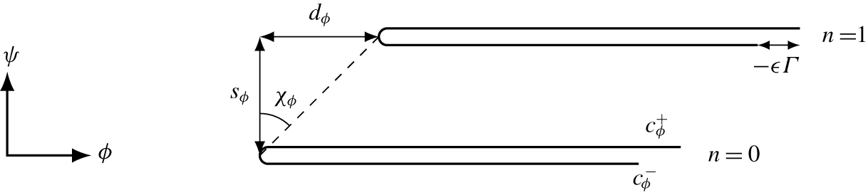
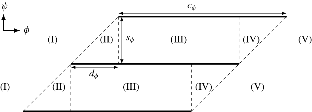
We immediately note that the angle of attack affects the blade spacing in  $(\unicode[STIX]{x1D719},\unicode[STIX]{x1D713})$-space and will accordingly influence the cut-on and cut-off frequencies of the acoustic modes. These new parameters are illustrated in figure 5.
Exponential decompositions of the complex velocity field  $q-\text{i}\unicode[STIX]{x1D707}$ are available in the upstream and downstream regions, and are detailed in §§ S:3 and S:6 of the supplementary material. Such a decomposition is essential for the application of the Wiener–Hopf method in § 3.2.
We define the location of the upper/lower side of the image of the trailing edge in  $(\unicode[STIX]{x1D719},\unicode[STIX]{x1D713})$-space as
 $(c_{\unicode[STIX]{x1D719}}^{\pm },0)$. It is important to note that the image of the physical trailing edge is not unique, but the upper and lower sides are in fact mapped to two different points. Formula (2.6) yields analytic expressions for the trailing-edge images as
 $$\begin{eqnarray}c_{\unicode[STIX]{x1D719}}^{\pm }=2(1-\text{i}\unicode[STIX]{x1D716}\unicode[STIX]{x1D6FC})-\frac{\unicode[STIX]{x1D716}}{2\unicode[STIX]{x03C0}\text{i}}\int _{0}^{2}\unicode[STIX]{x1D6FE}(\unicode[STIX]{x1D70F})\left(\log \left(\frac{\displaystyle \sinh \left(\frac{\unicode[STIX]{x03C0}\text{i}(\unicode[STIX]{x1D70F}-2)}{d+\text{i}s}\right)}{\displaystyle \sinh \left(\frac{\unicode[STIX]{x03C0}\text{i}\unicode[STIX]{x1D70F}}{d+\text{i}s}\right)}\right)\pm \unicode[STIX]{x03C0}\text{i}+\frac{2\unicode[STIX]{x03C0}\text{i}}{d+\text{i}s}\right)\,\text{d}\unicode[STIX]{x1D70F},\end{eqnarray}$$
which are both real numbers since the physical trailing edge  $(2,0^{\pm })$ lies on the same streamline as the origin. The difference between the location of the upper and lower trailing edges in
 $(\unicode[STIX]{x1D719},\unicode[STIX]{x1D713})$-space is
 $-\unicode[STIX]{x1D716}\unicode[STIX]{x1D6E4}$, which is the circulation around a single aerofoil, and may be calculated as
 $$\begin{eqnarray}\unicode[STIX]{x1D716}\unicode[STIX]{x1D6E4}=-\unicode[STIX]{x1D716}\int _{0}^{2}\unicode[STIX]{x1D6FE}(\unicode[STIX]{x1D70F})\,\text{d}\unicode[STIX]{x1D70F}=-\unicode[STIX]{x1D716}\unicode[STIX]{x03C0}\left(\unicode[STIX]{x1D6FE}_{r,0}+\frac{\unicode[STIX]{x1D6FE}_{r,1}}{2}\right),\end{eqnarray}$$
where  $\unicode[STIX]{x1D6FE}_{r,0}$ and
 $\unicode[STIX]{x1D6FE}_{r,1}$ are the first two coefficients of the weighted Chebyshev series defined in (S:3.6) in the supplementary material.
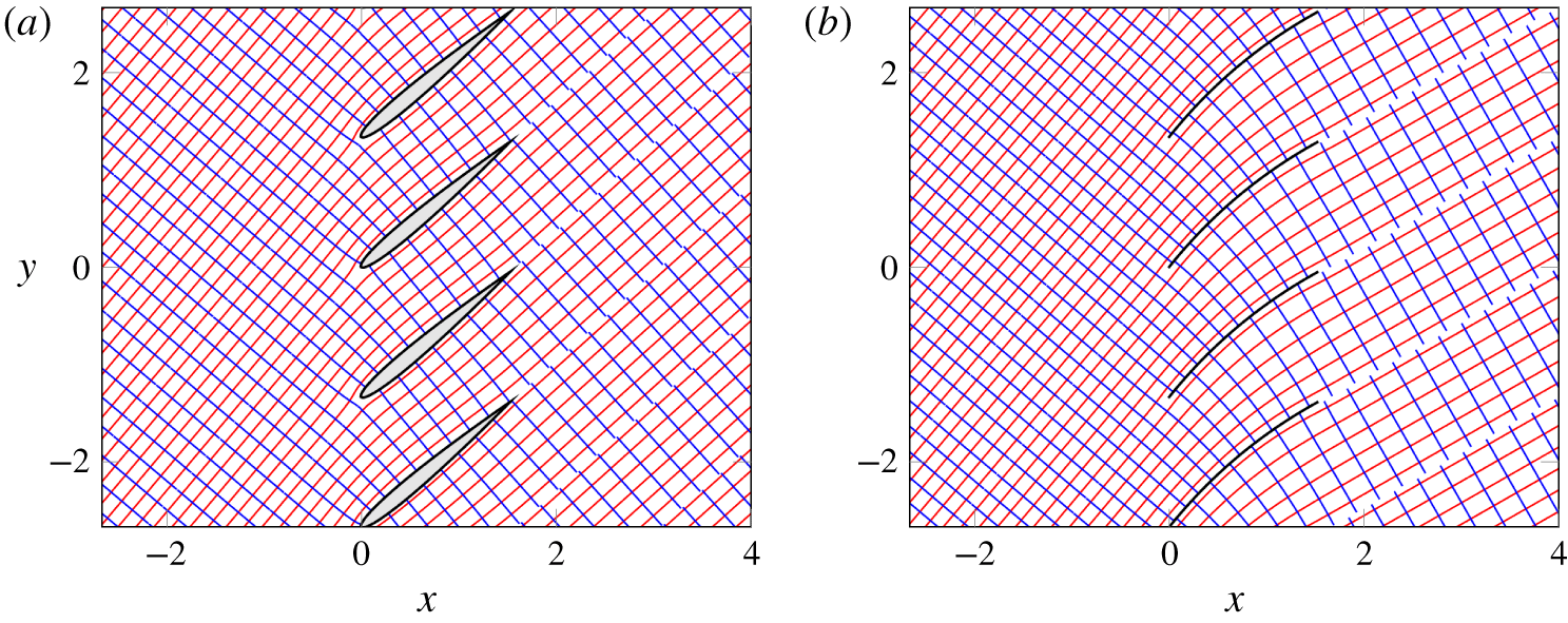
Contours of the velocity potential (blue) and streamfunction (red) for two cascades of aerofoils with gap-to-chord ratio  $\unicode[STIX]{x1D6E5}/2=2/3$, stagger angle
 $\unicode[STIX]{x1D712}=40^{\circ }$ and angle of attack
 $10^{\circ }$. (a) NACA 0008; (b) NACA 5500.

In figure 4 we plot the velocity potential and streamfunction contours for two aerofoil profiles at angle of attack  $10^{\circ }$: one with thickness (figure 4a) and one with camber (figure 4b). At this point, we highlight several features of the background flow in order to expedite the discussion of the aeroacoustic analysis in the following sections. Firstly, we note that the flow field satisfies the no-flux condition on the aerofoil surfaces and the Kutta condition at the aerofoil trailing edges. Secondly, the velocity potential and streamfunction are orthogonal everywhere and consequently form an orthogonal coordinate system. Thirdly, it can be seen that the thick aerofoils (figure 4a) scarcely deflect the flow whereas the cambered aerofoils (figure 4b) induce a significant flow deflection. The deflection angle is closely related to the aerofoil circulation (Baddoo & Ayton Reference Baddoo and Ayton2018b) and, accordingly, we observe a significant discontinuity in velocity potential across the wake in figure 4(b). In the following aeroacoustic analysis, this discontinuity must be regularised in order to ensure that the pressure field does not possess a jump across the wake.
Diagram showing parameters in the transformed  $(\unicode[STIX]{x1D719},\unicode[STIX]{x1D713})$-space.

2.2 Unsteady formulation
We now consider the unsteady interaction in the new, transformed coordinate system. The present analysis is restricted to inviscid linear disturbances of a two-dimensional irrotational compressible mean flow, using the formulation derived by Goldstein (Reference Goldstein1978) and further developed by Myers & Kerschen (Reference Myers and Kerschen1995). We assume that there are small amplitude vortical and entropic perturbations in the uniform flow far upstream of the cascade, which we denote by  $\boldsymbol{v}^{\prime }$ and
 $s^{\prime }$ respectively. These disturbances are convected downstream by the mean flow and interact with the cascade, thus producing sound. Similar approaches have been employed (Peake & Kerschen Reference Peake and Kerschen1997, Reference Peake and Kerschen2004; Evers & Peake Reference Evers and Peake2002) in modelling gust–cascade interaction. Unlike the flat-plate case (Glegg Reference Glegg1999), the mean flow modifies both the boundary conditions and governing equation. We will see that extra forcing terms are induced in the governing equation, while the boundary conditions include terms depending on the surface velocity.
The total unsteady velocity perturbation may be decomposed into the form (Goldstein Reference Goldstein1978)
 $$\begin{eqnarray}\boldsymbol{u}^{\prime }=\unicode[STIX]{x1D735}G^{\prime }+\boldsymbol{v}^{\prime },\end{eqnarray}$$
where  $\boldsymbol{v}^{\prime }$ satisfies a modified form of the linearised momentum equation. By employing the method of characteristics,
 $\boldsymbol{v}^{\prime }$ may be found exactly throughout the whole flow domain. The irrotational scattered field,
 $G^{\prime }$, then satisfies (Goldstein Reference Goldstein1978)
 $$\begin{eqnarray}\frac{\text{D}_{0}}{\text{D}t}\left(\frac{1}{c_{0}^{2}}\frac{\text{D}_{0}G^{\prime }}{\text{D}t}\right)-\frac{1}{\unicode[STIX]{x1D70C}_{0}}\unicode[STIX]{x1D735}\boldsymbol{\cdot }(\unicode[STIX]{x1D70C}_{0}\unicode[STIX]{x1D735}G^{\prime })=\frac{1}{\unicode[STIX]{x1D70C}_{0}}\unicode[STIX]{x1D735}\boldsymbol{\cdot }(\unicode[STIX]{x1D70C}_{0}\boldsymbol{v}^{\prime }),\end{eqnarray}$$
where the material derivative  $\text{D}_{0}/\text{D}t$ is taken with respect to the local mean flow. The quantities
 $\unicode[STIX]{x1D70C}_{0}$ and
 $c_{0}$ are the local values of density and speed of sound for the mean flow. The no-flux boundary condition on
 $G^{\prime }$ at any rigid surface is
 $$\begin{eqnarray}\frac{\unicode[STIX]{x2202}G^{\prime }}{\unicode[STIX]{x2202}n}=-\boldsymbol{v}^{\prime }\boldsymbol{\cdot }\boldsymbol{n},\end{eqnarray}$$
where  $\boldsymbol{n}$ is the unit normal vector.
The non-dimensional upstream velocity and entropy disturbances far upstream may be written as
 $$\begin{eqnarray}\left.\begin{array}{@{}c@{}}\displaystyle \boldsymbol{v}^{\prime }\rightarrow \unicode[STIX]{x1D708}\left[\begin{array}{@{}c@{}}A_{t}\\ A_{n}\\ A_{s}\end{array}\right]\text{e}^{\text{i}k(\unicode[STIX]{x1D719}+k_{n}\unicode[STIX]{x1D713}+k_{s}x_{3}-t)},\\ \displaystyle s^{\prime }\rightarrow 2\unicode[STIX]{x1D708}B\text{e}^{\text{i}k(\unicode[STIX]{x1D719}+k_{n}\unicode[STIX]{x1D713}+k_{s}x_{3}-t)},\end{array}\right\}\end{eqnarray}$$
subject to  $A_{t}+A_{n}k_{n}\unicode[STIX]{x1D6FD}_{\infty }+A_{s}k_{s}=0$, where
 $k=\unicode[STIX]{x1D714}b^{\ast }/U_{\infty }^{\ast }$ is the reduced frequency and time is normalised by
 $b^{\ast }/U_{\infty }^{\ast }$. The amplitude of the disturbance,
 $\unicode[STIX]{x1D708}$, is assumed to be small (
 $\unicode[STIX]{x1D708}\ll \unicode[STIX]{x1D716}$).
The transformation
 $$\begin{eqnarray}G^{\prime }(\unicode[STIX]{x1D719},\unicode[STIX]{x1D713})=h(\unicode[STIX]{x1D719},\unicode[STIX]{x1D713})\exp [\text{i}k(k_{3}x_{3}-t-\unicode[STIX]{x1D6FF}M_{\infty }^{2}\unicode[STIX]{x1D719})+\unicode[STIX]{x1D716}M_{\infty }^{2}q],\end{eqnarray}$$
allowed Kerschen & Myers (Reference Kerschen and Myers1987) to express Goldstein’s wave equation as
 $$\begin{eqnarray}\displaystyle & & \displaystyle \frac{\unicode[STIX]{x2202}^{2}h}{\unicode[STIX]{x2202}\unicode[STIX]{x1D719}^{2}}+\frac{\unicode[STIX]{x2202}^{2}h}{\unicode[STIX]{x2202}\unicode[STIX]{x1D713}^{2}}+k^{2}w^{2}h+\unicode[STIX]{x1D716}(\unicode[STIX]{x1D6FE}+1)M_{\infty }^{4}\unicode[STIX]{x1D6FF}\left\{q\left[\frac{\unicode[STIX]{x2202}^{2}h}{\unicode[STIX]{x2202}\unicode[STIX]{x1D713}^{2}}+2\text{i}k\unicode[STIX]{x1D6FF}\frac{\unicode[STIX]{x2202}h}{\unicode[STIX]{x2202}\unicode[STIX]{x1D719}}+k^{2}(w^{2}+\unicode[STIX]{x1D6FF}^{2})h\right]\right.\nonumber\\ \displaystyle & & \displaystyle \quad -\left.\frac{\unicode[STIX]{x2202}q}{\unicode[STIX]{x2202}\unicode[STIX]{x1D719}}\left[\frac{\unicode[STIX]{x2202}h}{\unicode[STIX]{x2202}\unicode[STIX]{x1D719}}-\text{i}k\unicode[STIX]{x1D6FF}h\right]\right\}-\unicode[STIX]{x1D716}2k^{2}w^{2}\unicode[STIX]{x1D6FD}_{\infty }^{2}qh=\unicode[STIX]{x1D716}kS(\unicode[STIX]{x1D719},\unicode[STIX]{x1D713})\text{e}^{\text{i}k\unicode[STIX]{x1D6FA}},\end{eqnarray}$$
where
 $$\begin{eqnarray}\left.\begin{array}{@{}c@{}}\displaystyle \begin{array}{@{}c@{}}\unicode[STIX]{x1D6FA}=\unicode[STIX]{x1D6FF}\unicode[STIX]{x1D719}+k_{n}\unicode[STIX]{x1D713}+\unicode[STIX]{x1D716}g(\unicode[STIX]{x1D719},\unicode[STIX]{x1D713}),\quad w^{2}=(\unicode[STIX]{x1D6FF}M_{\infty })^{2}-(k_{s}/\unicode[STIX]{x1D6FD}_{\infty })^{2},\\ \displaystyle \unicode[STIX]{x1D6FF}=1/\unicode[STIX]{x1D6FD}_{\infty }^{2},\quad \tilde{A}_{t}=A_{t}-B,\end{array}\\ \displaystyle \begin{array}{@{}rcl@{}}\displaystyle S(\unicode[STIX]{x1D719},\unicode[STIX]{x1D713})\; & =\; & \displaystyle 2\unicode[STIX]{x1D6FF}\left\{\text{i}(\tilde{A}_{t}-k_{n}A_{n}\unicode[STIX]{x1D6FD}_{\infty }^{3})q+\text{i}(k_{n}\tilde{A}_{t}\unicode[STIX]{x1D6FD}_{\infty }+A_{n}\unicode[STIX]{x1D6FD}_{\infty })\unicode[STIX]{x1D707}\right.\\ \; & \; & \displaystyle +\left.\frac{1}{k}\left[\tilde{A}_{t}M_{\infty }^{2}\frac{\unicode[STIX]{x2202}q}{\unicode[STIX]{x2202}\unicode[STIX]{x1D719}}+A_{n}M_{\infty }^{2}\unicode[STIX]{x1D6FD}_{\infty }\frac{\unicode[STIX]{x2202}q}{\unicode[STIX]{x2202}\unicode[STIX]{x1D713}}\right]\right\},\end{array}\end{array}\right\}\end{eqnarray}$$
and  $g$ is Lighthill’s drift function, which represents the cumulative distortion of vortex filaments by the non-uniform mean flow,
 $$\begin{eqnarray}g(\unicode[STIX]{x1D719},\unicode[STIX]{x1D713})=\int _{-\infty }^{\unicode[STIX]{x1D719}}\left[\frac{1}{U_{0}^{2}(\unicode[STIX]{x1D702},\unicode[STIX]{x1D713})}-1\right]\,\text{d}\unicode[STIX]{x1D702}=-2\int _{-\infty }^{\unicode[STIX]{x1D719}}q(\unicode[STIX]{x1D702},\unicode[STIX]{x1D713})\,\text{d}\unicode[STIX]{x1D702}.\end{eqnarray}$$
The no-flux boundary condition applied to rigid surfaces (2.10c) becomes
 $$\begin{eqnarray}\frac{\unicode[STIX]{x2202}h}{\unicode[STIX]{x2202}\unicode[STIX]{x1D713}}+\unicode[STIX]{x1D716}M_{\infty }^{2}\frac{\unicode[STIX]{x2202}q}{\unicode[STIX]{x2202}\unicode[STIX]{x1D713}}h=-\left[\frac{A_{n}}{\unicode[STIX]{x1D6FD}_{\infty }}(1-\unicode[STIX]{x1D716}M_{\infty }^{2}q)-\unicode[STIX]{x1D716}2\tilde{A}_{t}\unicode[STIX]{x1D707}\right]\text{e}^{\text{i}k\unicode[STIX]{x1D6FA}},\end{eqnarray}$$
applied on the body surface.
We will use the modified pressure  $p$, which is defined in terms of actual pressure
 $p^{\prime }$ as
 $$\begin{eqnarray}p=-p^{\prime }\text{e}^{\text{i}k(-k_{s}x_{3}+t)}=\frac{\unicode[STIX]{x2202}}{\unicode[STIX]{x2202}\unicode[STIX]{x1D719}}(h\text{e}^{-\text{i}k\unicode[STIX]{x1D6FF}\unicode[STIX]{x1D719}})\text{e}^{\text{i}k\unicode[STIX]{x1D719}}.\end{eqnarray}$$
2.3 Boundary conditions
We must specify an adequate number of boundary conditions in order for the problem to be well posed and physically valid. The boundary conditions are applied to each streamline that correspond to a blade surface, i.e.  $\unicode[STIX]{x1D713}=ns_{\unicode[STIX]{x1D719}}$ for integer
 $n$. Upstream of the blade, we require that there are no discontinuities across this streamline. On the blade itself, the no-flux condition for a rigid surface (2.16) must be satisfied either side of the blade. Downstream of the blade, we require two conditions – firstly the jump in normal velocity either side of the wake must vanish, and secondly, there can be no pressure jump across the wake. Due to the disparity between the images of the upper and lower trailing edge, which is equal to the mean flow circulation, some care is required with these latter two boundary conditions. The full set of boundary conditions is summarised and illustrated in figure 6.
As previously mentioned in (2.8), there are two trailing edges  $c_{\unicode[STIX]{x1D719}}^{\pm }$ in the parametric
 $(\unicode[STIX]{x1D719},\unicode[STIX]{x1D713})$-space. In the application of the boundary conditions, we define a single trailing edge at
 $c_{\unicode[STIX]{x1D719}}=c_{\unicode[STIX]{x1D719}}^{+}$. This produces
 $O(\unicode[STIX]{x1D716})$ errors, which will be corrected in our asymptotic expansion later.
In the following analysis, we use  $\unicode[STIX]{x1D6E5}_{n}$ and
 $\unicode[STIX]{x1D6F4}_{n}$ to denote the difference and sum of a given quantity either side of the
 $n$th aerofoil’s streamline.
Schematic illustrating where each boundary condition is applied.

2.3.1 Upstream boundary condition
The condition of no upstream discontinuities is simply
 $$\begin{eqnarray}\unicode[STIX]{x1D6E5}_{n}[h](\unicode[STIX]{x1D719})=0,\quad \text{for }\unicode[STIX]{x1D719}<0.\end{eqnarray}$$
2.3.2 No-flux boundary conditions
The flow on each side of the blade must satisfy the rigid surface condition (2.16) which, after ignoring  $O(\unicode[STIX]{x1D716}^{2})$ terms, becomes
 $$\begin{eqnarray}\displaystyle & & \displaystyle \frac{\unicode[STIX]{x2202}h^{\pm }}{\unicode[STIX]{x2202}\unicode[STIX]{x1D713}}(\unicode[STIX]{x1D719})+\unicode[STIX]{x1D716}M_{\infty }^{2}\frac{\unicode[STIX]{x2202}q^{\pm }}{\unicode[STIX]{x2202}\unicode[STIX]{x1D713}}(\unicode[STIX]{x1D719})h^{\pm }(\unicode[STIX]{x1D719})\end{eqnarray}$$
 $$\begin{eqnarray}\displaystyle & & \displaystyle \quad =-\left[\frac{A_{n}}{\unicode[STIX]{x1D6FD}_{\infty }}(1-\unicode[STIX]{x1D716}M_{\infty }^{2}q^{\pm }(\unicode[STIX]{x1D719})+\unicode[STIX]{x1D716}\text{i}kg^{\pm }(\unicode[STIX]{x1D719}))-\unicode[STIX]{x1D716}2\tilde{A}_{t}\unicode[STIX]{x1D707}^{\pm }(\unicode[STIX]{x1D719})\right]\text{e}^{\text{i}k\unicode[STIX]{x1D6FF}\unicode[STIX]{x1D719}},\quad 0<\unicode[STIX]{x1D719}<c_{\unicode[STIX]{x1D719}},\nonumber\\ \displaystyle & & \displaystyle\end{eqnarray}$$
where we have assumed that  $\unicode[STIX]{x1D716}k\ll 1$. This linearisation corresponds to step IIa in the road map.
2.3.3 Wake boundary conditions
We now derive the boundary conditions to be applied on the aerofoil wake. This corresponds to step IIb in the road map. The lower trailing edge lags behind the upper trailing edge in  $(\unicode[STIX]{x1D719},\unicode[STIX]{x1D713})$-space by a distance of
 $-\unicode[STIX]{x1D716}\unicode[STIX]{x1D6E4}$, as illustrated in figures 5 and 6. Consequently, the condition of continuity of normal velocity in terms of our acoustic potential function is
 $$\begin{eqnarray}\frac{\unicode[STIX]{x2202}h^{+}}{\unicode[STIX]{x2202}\unicode[STIX]{x1D713}}(\unicode[STIX]{x1D719})\text{e}^{-\text{i}kM_{\infty }^{2}\unicode[STIX]{x1D6FF}\unicode[STIX]{x1D719}}-\frac{\unicode[STIX]{x2202}h^{-}}{\unicode[STIX]{x2202}\unicode[STIX]{x1D713}}(\unicode[STIX]{x1D719}+\unicode[STIX]{x1D716}\unicode[STIX]{x1D6E4})\text{e}^{-\text{i}kM_{\infty }^{2}\unicode[STIX]{x1D6FF}(\unicode[STIX]{x1D719}+\unicode[STIX]{x1D716}\unicode[STIX]{x1D6E4})}=0,\quad \text{for }\unicode[STIX]{x1D719}>c_{\unicode[STIX]{x1D719}}.\end{eqnarray}$$
We may Taylor expand the second term about  $\unicode[STIX]{x1D719}$ to give
 $$\begin{eqnarray}\frac{\unicode[STIX]{x2202}h^{+}}{\unicode[STIX]{x2202}\unicode[STIX]{x1D713}}(\unicode[STIX]{x1D719})-\left(\frac{\unicode[STIX]{x2202}h^{-}}{\unicode[STIX]{x2202}\unicode[STIX]{x1D713}}(\unicode[STIX]{x1D719})+\unicode[STIX]{x1D716}\unicode[STIX]{x1D6E4}\frac{\unicode[STIX]{x2202}^{2}h^{-}}{\unicode[STIX]{x2202}\unicode[STIX]{x1D719}\unicode[STIX]{x2202}\unicode[STIX]{x1D713}}(\unicode[STIX]{x1D719})\right)(1-\text{i}kM_{\infty }^{2}\unicode[STIX]{x1D6FF}\unicode[STIX]{x1D716}\unicode[STIX]{x1D6E4})=0,\end{eqnarray}$$
where we have assumed that  $\unicode[STIX]{x1D716}kM_{\infty }^{2}\ll 1$ and ignored
 $O(\unicode[STIX]{x1D716}^{2})$ terms. We accordingly obtain the condition on the jump in normal velocity in
 $(\unicode[STIX]{x1D719},\unicode[STIX]{x1D713})$-space as
 $$\begin{eqnarray}\unicode[STIX]{x1D6E5}_{n}\left[\frac{\unicode[STIX]{x2202}h}{\unicode[STIX]{x2202}\unicode[STIX]{x1D713}}\right](\unicode[STIX]{x1D719})=\unicode[STIX]{x1D716}\unicode[STIX]{x1D6E4}\left(\frac{\unicode[STIX]{x2202}^{2}h^{-}}{\unicode[STIX]{x2202}\unicode[STIX]{x1D719}\unicode[STIX]{x2202}\unicode[STIX]{x1D713}}(\unicode[STIX]{x1D719})-\text{i}kM_{\infty }^{2}\unicode[STIX]{x1D6FF}\frac{\unicode[STIX]{x2202}h^{-}}{\unicode[STIX]{x2202}\unicode[STIX]{x1D713}}(\unicode[STIX]{x1D719})\right),\quad \text{for }\unicode[STIX]{x1D719}>c_{\unicode[STIX]{x1D719}}.\end{eqnarray}$$
Using a similar method, we reformulate the pressure continuity condition in  $(\unicode[STIX]{x1D719},\unicode[STIX]{x1D713})$-space. Due to the lag in the lower trailing-edge location, we may write
 $$\begin{eqnarray}p^{\prime +}(\unicode[STIX]{x1D719})-p^{\prime -}(\unicode[STIX]{x1D719}+\unicode[STIX]{x1D716}\unicode[STIX]{x1D6E4})=0,\quad \text{for }\unicode[STIX]{x1D719}>c_{\unicode[STIX]{x1D719}}.\end{eqnarray}$$
Taylor expanding the latter term about  $\unicode[STIX]{x1D719}$ and ignoring terms of
 $O(\unicode[STIX]{x1D716}^{2})$ yields
 $$\begin{eqnarray}p^{\prime +}(\unicode[STIX]{x1D719})-p^{\prime -}(\unicode[STIX]{x1D719})-\unicode[STIX]{x1D716}\unicode[STIX]{x1D6E4}\frac{\unicode[STIX]{x2202}p^{\prime -}}{\unicode[STIX]{x2202}\unicode[STIX]{x1D719}}(\unicode[STIX]{x1D719})=0.\end{eqnarray}$$
By substituting (2.17) and cancelling terms, we obtain
 $$\begin{eqnarray}\frac{\unicode[STIX]{x2202}}{\unicode[STIX]{x2202}\unicode[STIX]{x1D719}}(\unicode[STIX]{x1D6E5}_{n}[h](\unicode[STIX]{x1D719})\text{e}^{-\text{i}k\unicode[STIX]{x1D6FF}\unicode[STIX]{x1D719}})\text{e}^{\text{i}k\unicode[STIX]{x1D719}}-\unicode[STIX]{x1D716}\unicode[STIX]{x1D6E4}\frac{\unicode[STIX]{x2202}}{\unicode[STIX]{x2202}\unicode[STIX]{x1D719}}\left(\frac{\unicode[STIX]{x2202}}{\unicode[STIX]{x2202}\unicode[STIX]{x1D719}}(h^{-}(\unicode[STIX]{x1D719})\text{e}^{-\text{i}k\unicode[STIX]{x1D6FF}\unicode[STIX]{x1D719}})\text{e}^{\text{i}k\unicode[STIX]{x1D719}}\right)=0.\end{eqnarray}$$
We may integrate the above expression to obtain the condition on the jump in acoustic potential in  $(\unicode[STIX]{x1D719},\unicode[STIX]{x1D713})$-space as
 $$\begin{eqnarray}\unicode[STIX]{x1D6E5}_{n}[h](\unicode[STIX]{x1D719})=2\unicode[STIX]{x03C0}\text{i}P\text{e}^{\text{i}k\unicode[STIX]{x1D6FF}\unicode[STIX]{x1D719}}+\unicode[STIX]{x1D716}\unicode[STIX]{x1D6E4}\left(\frac{\unicode[STIX]{x2202}h^{-}}{\unicode[STIX]{x2202}\unicode[STIX]{x1D719}}(\unicode[STIX]{x1D719})-\text{i}kM_{\infty }^{2}\unicode[STIX]{x1D6FF}h^{-}(\unicode[STIX]{x1D719})\right),\quad \text{for }\unicode[STIX]{x1D719}>c_{\unicode[STIX]{x1D719}},\end{eqnarray}$$
where  $P$ is a constant of integration that will be determined by the Wiener–Hopf technique.
3 Acoustic scattered solution
We now seek a regular perturbation expansion in  $\unicode[STIX]{x1D716}$ for
 $h$ as
 $$\begin{eqnarray}h(\unicode[STIX]{x1D719},\unicode[STIX]{x1D713})\sim h_{0}(\unicode[STIX]{x1D719},\unicode[STIX]{x1D713})+\unicode[STIX]{x1D716}h_{1}(\unicode[STIX]{x1D719},\unicode[STIX]{x1D713})+\cdots \,.\end{eqnarray}$$
This corresponds to step III in the road map. We now separate the  $O(1)$ and
 $O(\unicode[STIX]{x1D716})$ problems in order to generate an integral equation for the
 $O(\unicode[STIX]{x1D716})$ problem (road map step IV). The asymptotic expansion results in a pair of equations for the first- and second-order expansions of
 $h$,
 $$\begin{eqnarray}\displaystyle & \displaystyle O(1):\quad {\mathcal{L}}(h_{0})=0, & \displaystyle\end{eqnarray}$$
 $$\begin{eqnarray}\displaystyle & \displaystyle O(\unicode[STIX]{x1D716}):\quad {\mathcal{L}}(h_{1})=\mathbb{S}(\unicode[STIX]{x1D719},\unicode[STIX]{x1D713}), & \displaystyle\end{eqnarray}$$
 $$\begin{eqnarray}{\mathcal{L}}(f)=\frac{\unicode[STIX]{x2202}^{2}f}{\unicode[STIX]{x2202}\unicode[STIX]{x1D719}^{2}}+\frac{\unicode[STIX]{x2202}^{2}f}{\unicode[STIX]{x2202}\unicode[STIX]{x1D713}^{2}}+k^{2}w^{2}f,\end{eqnarray}$$
and the forcing term is
 $$\begin{eqnarray}\displaystyle \mathbb{S}(\unicode[STIX]{x1D719},\unicode[STIX]{x1D713}) & = & \displaystyle kS(\unicode[STIX]{x1D719},\unicode[STIX]{x1D713})\text{e}^{\text{i}k\unicode[STIX]{x1D6FA}}-(\unicode[STIX]{x1D6FE}+1)M_{\infty }^{4}\unicode[STIX]{x1D6FF}\left\{q\left[\frac{\unicode[STIX]{x2202}^{2}h_{0}}{\unicode[STIX]{x2202}\unicode[STIX]{x1D713}^{2}}+2\text{i}k\unicode[STIX]{x1D6FF}\frac{\unicode[STIX]{x2202}h_{0}}{\unicode[STIX]{x2202}\unicode[STIX]{x1D719}}+k^{2}(w^{2}+\unicode[STIX]{x1D6FF}^{2})h_{0}\right]\right.\nonumber\\ \displaystyle & & \displaystyle -\left.\frac{\unicode[STIX]{x2202}q}{\unicode[STIX]{x2202}\unicode[STIX]{x1D719}}\left[\frac{\unicode[STIX]{x2202}h_{0}}{\unicode[STIX]{x2202}\unicode[STIX]{x1D719}}-\text{i}k\unicode[STIX]{x1D6FF}h_{0}\right]\right\}+2k^{2}w^{2}\unicode[STIX]{x1D6FD}_{\infty }^{2}qh_{0}.\end{eqnarray}$$
The condition of no discontinuities upstream of the cascade simply becomes
 $$\begin{eqnarray}\displaystyle & \displaystyle \unicode[STIX]{x1D6E5}_{0}[h_{0}](\unicode[STIX]{x1D719})=0,\quad \text{for }\unicode[STIX]{x1D719}<0, & \displaystyle\end{eqnarray}$$
 $$\begin{eqnarray}\displaystyle & \displaystyle \unicode[STIX]{x1D6E5}_{0}[h_{1}](\unicode[STIX]{x1D719})=0,\quad \text{for }\unicode[STIX]{x1D719}<0. & \displaystyle\end{eqnarray}$$
 $\unicode[STIX]{x1D6F4}_{0}$) or difference (
 $\unicode[STIX]{x1D6E5}_{0}$) either side of the blade. To further facilitate the Wiener–Hopf analysis, we expand the boundary data in terms of a Fourier series (step IVa of the road map). The anti-symmetric boundary data become
 $$\begin{eqnarray}\displaystyle & \displaystyle \unicode[STIX]{x1D6E5}_{0}\left[\frac{\unicode[STIX]{x2202}h_{0}}{\unicode[STIX]{x2202}\unicode[STIX]{x1D713}}\right](\unicode[STIX]{x1D719})=0,\quad 0<\unicode[STIX]{x1D719}<c_{\unicode[STIX]{x1D719}}, & \displaystyle\end{eqnarray}$$
 $$\begin{eqnarray}\displaystyle & \displaystyle \unicode[STIX]{x1D6E5}_{0}\left[\frac{\unicode[STIX]{x2202}h_{1}}{\unicode[STIX]{x2202}\unicode[STIX]{x1D713}}\right](\unicode[STIX]{x1D719})=\mathop{\sum }_{l=-\infty }^{\infty }{\mathcal{c}}_{\unicode[STIX]{x1D6E5},l}\text{e}^{-\text{i}\unicode[STIX]{x1D705}_{l}^{-}\unicode[STIX]{x1D719}},\quad 0<\unicode[STIX]{x1D719}<c_{\unicode[STIX]{x1D719}}, & \displaystyle\end{eqnarray}$$
where  $\unicode[STIX]{x1D705}_{l}^{-}=-k\unicode[STIX]{x1D6FF}+l\unicode[STIX]{x03C0}/c_{\unicode[STIX]{x1D719}}$. The Fourier coefficients are defined using (2.20) as
 $$\begin{eqnarray}{\mathcal{c}}_{\unicode[STIX]{x1D6E5},l}=\frac{1}{c_{\unicode[STIX]{x1D719}}}\int _{0}^{c_{\unicode[STIX]{x1D719}}}\unicode[STIX]{x1D6E5}_{0}\left[\frac{\unicode[STIX]{x2202}h_{1}}{\unicode[STIX]{x2202}\unicode[STIX]{x1D713}}\right](\unicode[STIX]{x1D719})\cos \left(\frac{l\unicode[STIX]{x03C0}\unicode[STIX]{x1D719}}{c_{\unicode[STIX]{x1D719}}}\right)\text{e}^{\text{i}\unicode[STIX]{x1D705}_{0}^{-}\unicode[STIX]{x1D719}}\,\text{d}\unicode[STIX]{x1D719},\end{eqnarray}$$
which also accounts for the  $\unicode[STIX]{x1D716}M_{\infty }^{2}(\unicode[STIX]{x2202}q^{\pm }/\unicode[STIX]{x2202}\unicode[STIX]{x1D713})(\unicode[STIX]{x1D719})h_{0}^{\pm }(\unicode[STIX]{x1D719})$ terms taken to the right-hand side of (2.20), which may be considered as known due to the perturbation expansion. Note that the periodicity of this Fourier series is
 $2c_{\unicode[STIX]{x1D719}}$ to ensure a good approximation at the leading and trailing edges.
Similarly, we may write the symmetric data in the no-flux condition (2.20) as
 $$\begin{eqnarray}\displaystyle & \displaystyle \unicode[STIX]{x1D6F4}_{0}\left[\frac{\unicode[STIX]{x2202}h_{0}}{\unicode[STIX]{x2202}\unicode[STIX]{x1D713}}\right](\unicode[STIX]{x1D719})=-2\frac{A_{n}}{\unicode[STIX]{x1D6FD}_{\infty }}\text{e}^{\text{i}k\unicode[STIX]{x1D6FF}\unicode[STIX]{x1D719}},\quad 0<\unicode[STIX]{x1D719}<c_{\unicode[STIX]{x1D719}}, & \displaystyle\end{eqnarray}$$
 $$\begin{eqnarray}\displaystyle & \displaystyle \unicode[STIX]{x1D6F4}_{0}\left[\frac{\unicode[STIX]{x2202}h_{1}}{\unicode[STIX]{x2202}\unicode[STIX]{x1D713}}\right](\unicode[STIX]{x1D719})=\mathop{\sum }_{l=-\infty }^{\infty }{\mathcal{c}}_{\unicode[STIX]{x1D6F4},l}\text{e}^{-\text{i}\unicode[STIX]{x1D705}_{l}^{-}\unicode[STIX]{x1D719}},\quad 0<\unicode[STIX]{x1D719}<c_{\unicode[STIX]{x1D719}}, & \displaystyle\end{eqnarray}$$
where the Fourier coefficients are defined using (2.20) as
 $$\begin{eqnarray}{\mathcal{c}}_{\unicode[STIX]{x1D6F4},l}=\frac{1}{c_{\unicode[STIX]{x1D719}}}\int _{0}^{c_{\unicode[STIX]{x1D719}}}\unicode[STIX]{x1D6F4}_{0}\left[\frac{\unicode[STIX]{x2202}h_{1}}{\unicode[STIX]{x2202}\unicode[STIX]{x1D713}}\right](\unicode[STIX]{x1D719})\cos \left(\frac{l\unicode[STIX]{x03C0}\unicode[STIX]{x1D719}}{c_{\unicode[STIX]{x1D719}}}\right)\text{e}^{\text{i}\unicode[STIX]{x1D705}_{0}^{-}\unicode[STIX]{x1D719}}\,\text{d}\unicode[STIX]{x1D719}.\end{eqnarray}$$
Combining the anti-symmetric ((3.6a), (3.6b)) and symmetric ((3.7a), (3.7b)) data yield the original no-flux condition (2.20).
Applying the perturbation expansion to continuity of normal velocity across the wake (2.23) and equating terms of equal order gives
 $$\begin{eqnarray}\displaystyle & \displaystyle \unicode[STIX]{x1D6E5}_{0}\left[\frac{\unicode[STIX]{x2202}h_{0}}{\unicode[STIX]{x2202}\unicode[STIX]{x1D713}}\right](\unicode[STIX]{x1D719})=0, & \displaystyle\end{eqnarray}$$
 $$\begin{eqnarray}\displaystyle & \displaystyle \unicode[STIX]{x1D6E5}_{0}\left[\frac{\unicode[STIX]{x2202}h_{1}}{\unicode[STIX]{x2202}\unicode[STIX]{x1D713}}\right](\unicode[STIX]{x1D719})=\unicode[STIX]{x1D6E4}\left(\frac{\unicode[STIX]{x2202}^{2}h^{-}}{\unicode[STIX]{x2202}\unicode[STIX]{x1D719}\unicode[STIX]{x2202}\unicode[STIX]{x1D713}}(\unicode[STIX]{x1D719})-\text{i}kM_{\infty }^{2}\unicode[STIX]{x1D6FF}\frac{\unicode[STIX]{x2202}h^{-}}{\unicode[STIX]{x2202}\unicode[STIX]{x1D713}}(\unicode[STIX]{x1D719})\right),\quad \unicode[STIX]{x1D719}>c_{\unicode[STIX]{x1D719}}. & \displaystyle\end{eqnarray}$$
 $$\begin{eqnarray}\displaystyle & \displaystyle \unicode[STIX]{x1D6E5}_{0}[h_{0}](\unicode[STIX]{x1D719})=2\unicode[STIX]{x03C0}\text{i}P_{0}\text{e}^{-\text{i}\unicode[STIX]{x1D705}_{0}^{-}\unicode[STIX]{x1D719}},\quad \unicode[STIX]{x1D719}>c_{\unicode[STIX]{x1D719}}, & \displaystyle\end{eqnarray}$$
 $$\begin{eqnarray}\displaystyle & \displaystyle \unicode[STIX]{x1D6E5}_{0}[h_{1}](\unicode[STIX]{x1D719})=2\unicode[STIX]{x03C0}\text{i}P_{1}\text{e}^{-\text{i}\unicode[STIX]{x1D705}_{0}^{-}\unicode[STIX]{x1D719}}+\unicode[STIX]{x1D6E4}\left(\frac{\unicode[STIX]{x2202}h^{-}}{\unicode[STIX]{x2202}\unicode[STIX]{x1D719}}(\unicode[STIX]{x1D719})-\text{i}kM_{\infty }^{2}\unicode[STIX]{x1D6FF}h^{-}(\unicode[STIX]{x1D719})\right),\quad \unicode[STIX]{x1D719}>c_{\unicode[STIX]{x1D719}}, & \displaystyle\end{eqnarray}$$
 $P_{0}$ and
 $P_{1}$ are constants of integration to be determined by the unsteady Kutta condition (Ayton, Gill & Peake Reference Ayton, Gill and Peake2016).
3.1 Solution to  $O(1)$ problem

The  $O(1)$ system of equations ((3.2a), (3.5a), (3.6a), (3.7a), (3.8a), (3.9a)) was considered by Glegg (Reference Glegg1999) and Posson et al. (Reference Posson, Roger and Moreau2010). This corresponds to step IVb in the road map. The solution is written in terms of the
 $\unicode[STIX]{x1D719}$-Fourier transform of the jump in potential either side of the blade and wake,
 $$\begin{eqnarray}D_{0}(\unicode[STIX]{x1D6FE})=\frac{1}{2\unicode[STIX]{x03C0}}\int _{0}^{\infty }\unicode[STIX]{x1D6E5}_{0}[h_{0}](\unicode[STIX]{x1D719})\text{e}^{\text{i}\unicode[STIX]{x1D6FE}\unicode[STIX]{x1D719}}\,\text{d}\unicode[STIX]{x1D719},\end{eqnarray}$$
and the solution is
 $$\begin{eqnarray}\displaystyle D_{0}(\unicode[STIX]{x1D6FE}) & = & \displaystyle \frac{-\text{i}A_{n}}{\unicode[STIX]{x1D6FD}_{\infty }(2\unicode[STIX]{x03C0})^{2}(\unicode[STIX]{x1D6FE}-\unicode[STIX]{x1D705}_{0}^{-})J_{+}(\unicode[STIX]{x1D6FE})J_{-}(\unicode[STIX]{x1D705}_{0}^{-})}-\mathop{\sum }_{n=0}^{\infty }\frac{({\mathcal{A}}_{0,n}+{\mathcal{C}}_{0,n})\text{e}^{\text{i}(\unicode[STIX]{x1D6FE}-\unicode[STIX]{x1D703}_{n}^{-})c_{\unicode[STIX]{x1D719}}}}{\text{i}(\unicode[STIX]{x1D6FE}-\unicode[STIX]{x1D705}_{0}^{-})(\unicode[STIX]{x1D6FE}-\unicode[STIX]{x1D703}_{n}^{-})}\cdot \frac{J_{-}(\unicode[STIX]{x1D703}_{n}^{-})}{J_{-}(\unicode[STIX]{x1D6FE})}\nonumber\\ \displaystyle & & \displaystyle -\,\mathop{\sum }_{n=0}^{\infty }\frac{{\mathcal{B}}_{0,n}}{(\unicode[STIX]{x1D6FE}-\unicode[STIX]{x1D703}_{n}^{+})}\cdot \frac{J_{+}(\unicode[STIX]{x1D703}_{n}^{+})}{J_{+}(\unicode[STIX]{x1D6FE})},\end{eqnarray}$$
where all undefined terms may be found in the supplementary material. The function  $D_{0}(\unicode[STIX]{x1D6FE})$ was found by Glegg (Reference Glegg1999), and the Fourier transform was inverted to provide the acoustic field in the upstream and downstream regions. The acoustic field in the inter-blade region was found by Posson et al. (Reference Posson, Roger and Moreau2010) by choosing an appropriate contour of integration dependent on the region in the channel where the acoustic field was to be evaluated.
3.2 Solution to $O(\unicode[STIX]{x1D716})$ problem

Having solved the  $O(1)$ equation, we now move on to the
 $O(\unicode[STIX]{x1D716})$ equation. In particular, we seek to generate an integral equation that will be amenable to the Wiener–Hopf method. Following Glegg (Reference Glegg1999), we seek a solution using integral transforms. Currently,
 $h_{1}$ has a discontinuity across each blade and wake and consequently its derivatives are not integrable. Therefore, we introduce generalised derivatives (Lighthill Reference Lighthill1958) such that the Laplacian operator becomes
 $$\begin{eqnarray}\unicode[STIX]{x1D6FB}^{2}h_{1}=\tilde{\unicode[STIX]{x1D6FB}}^{2}h_{1}-\mathop{\sum }_{n=-\infty }^{\infty }\unicode[STIX]{x1D6E5}_{n}[h_{1}](\unicode[STIX]{x1D719})\unicode[STIX]{x1D6FF}^{\prime }(\unicode[STIX]{x1D713}-ns_{\unicode[STIX]{x1D719}})-\mathop{\sum }_{n=-\infty }^{\infty }\unicode[STIX]{x1D6E5}_{n}\left[\frac{\unicode[STIX]{x2202}h_{1}}{\unicode[STIX]{x2202}\unicode[STIX]{x1D713}}\right](\unicode[STIX]{x1D719})\unicode[STIX]{x1D6FF}(\unicode[STIX]{x1D713}-ns_{\unicode[STIX]{x1D719}}),\end{eqnarray}$$
where  $\tilde{\unicode[STIX]{x1D6FB}}^{2}$ represents the Laplacian operator with discontinuities removed, the second term on the right represents the discontinuity of acoustic potential either side of the blade and wake and the third term on the right represents the discontinuity of normal velocity either side of the blade and wake. This step corresponds to step IVc in the road map. Crucially, the above is expressed in the
 $(\unicode[STIX]{x1D719},\unicode[STIX]{x1D713})$-space, not in physical space.
In Glegg (Reference Glegg1999), the last term in (3.12) disappears on the aerofoil surfaces because the blades are infinitesimally thin, so there is no jump in the normal velocity either side of the blade. However, although the blades are ‘thin’ in our  $(\unicode[STIX]{x1D719},\unicode[STIX]{x1D713})$-space, they have been converted from thick blades in physical space, and therefore will induce some mass flux in order to satisfy the no-flux condition in the physical domain. Also, in Glegg (Reference Glegg1999), the last term in (3.12) disappears along the wake, because it is not a source of mass injection. Whilst this condition is true in our case in physical space, the mean flow circulation has induced a shift in the upper and lower trailing edges in the
 $(\unicode[STIX]{x1D719},\unicode[STIX]{x1D713})$-space, so some mass injection is required in the transformed space in order to have continuous normal velocity in the physical space.
The jump in the acoustic potential across a blade streamline is unknown and must be found as part of the solution. Conversely, the jump in  $\unicode[STIX]{x1D713}$-derivative of the acoustic potential is known in terms of mean flow quantities and the
 $O(1)$ solution.
As is typical in cascade acoustics problems, we note that the periodicity of the background flow and gust furnishes a quasi-periodic condition on the physical unsteady potential,
 $$\begin{eqnarray}G^{\prime }(\unicode[STIX]{x1D719}+nd_{\unicode[STIX]{x1D719}},\unicode[STIX]{x1D713}+ns_{\unicode[STIX]{x1D719}})=G^{\prime }(\unicode[STIX]{x1D719},\unicode[STIX]{x1D713})\text{e}^{\text{i}n\unicode[STIX]{x1D70E}_{\unicode[STIX]{x1D719}}},\end{eqnarray}$$
where  $\unicode[STIX]{x1D70E}_{\unicode[STIX]{x1D719}}$ is the inter-blade phase angle of the gust in
 $(\unicode[STIX]{x1D719},\unicode[STIX]{x1D713})$-space so that
 $\unicode[STIX]{x1D70E}_{\unicode[STIX]{x1D719}}=k(d_{\unicode[STIX]{x1D719}}+k_{n}s_{\unicode[STIX]{x1D719}})$. The inter-blade phase angle in the physical domain,
 $\unicode[STIX]{x1D70E}$, is obtained using (2.7). In terms of the modified potential, this quasi-periodic condition becomes
 $$\begin{eqnarray}h_{1}(\unicode[STIX]{x1D719}+nd_{\unicode[STIX]{x1D719}},\unicode[STIX]{x1D713}+ns_{\unicode[STIX]{x1D719}})=h_{1}(\unicode[STIX]{x1D719},\unicode[STIX]{x1D713})\text{e}^{\text{i}n\unicode[STIX]{x1D70E}_{\unicode[STIX]{x1D719}}^{\prime }},\end{eqnarray}$$
where the modified inter-blade phase angle is  $\unicode[STIX]{x1D70E}_{\unicode[STIX]{x1D719}}^{\prime }=k(\unicode[STIX]{x1D6FF}d_{\unicode[STIX]{x1D719}}+k_{n}s_{\unicode[STIX]{x1D719}})$. We will use this relation repeatedly to reduce the problem from an infinite cascade to a strip of finite height. For example, by inserting (3.14) into the expression for the generalised Laplacian (3.12), we may rewrite the
 $O(\unicode[STIX]{x1D716})$ governing equation (3.2b) as
 $$\begin{eqnarray}\displaystyle \frac{\unicode[STIX]{x2202}^{2}h_{1}}{\unicode[STIX]{x2202}\unicode[STIX]{x1D719}^{2}}+\frac{\unicode[STIX]{x2202}^{2}h_{1}}{\unicode[STIX]{x2202}\unicode[STIX]{x1D713}^{2}}+k^{2}w^{2}h_{1} & = & \displaystyle \mathbb{S}(\unicode[STIX]{x1D719},\unicode[STIX]{x1D713})+\mathop{\sum }_{n=-\infty }^{\infty }\unicode[STIX]{x1D6E5}_{0}[h_{1}](\unicode[STIX]{x1D719}-nd_{\unicode[STIX]{x1D719}})\unicode[STIX]{x1D6FF}^{\prime }(\unicode[STIX]{x1D713}-ns_{\unicode[STIX]{x1D719}})\text{e}^{\text{i}n\unicode[STIX]{x1D70E}_{\unicode[STIX]{x1D719}}^{\prime }}\nonumber\\ \displaystyle & & \displaystyle +\,\mathop{\sum }_{n=-\infty }^{\infty }\unicode[STIX]{x1D6E5}_{0}\left[\frac{\unicode[STIX]{x2202}h_{1}}{\unicode[STIX]{x2202}\unicode[STIX]{x1D713}}\right](\unicode[STIX]{x1D719}-nd_{\unicode[STIX]{x1D719}})\unicode[STIX]{x1D6FF}(\unicode[STIX]{x1D713}-ns_{\unicode[STIX]{x1D719}})\text{e}^{\text{i}n\unicode[STIX]{x1D70E}_{\unicode[STIX]{x1D719}}^{\prime }}.\end{eqnarray}$$
We define the Fourier integral transform and its inverse as
 $$\begin{eqnarray}\left.\begin{array}{@{}c@{}}\displaystyle F(\unicode[STIX]{x1D6FE},\unicode[STIX]{x1D707})=\frac{1}{(2\unicode[STIX]{x03C0})^{2}}\int _{-\infty }^{\infty }\int _{-\infty }^{\infty }f(\unicode[STIX]{x1D719},\unicode[STIX]{x1D713})\text{e}^{\text{i}\unicode[STIX]{x1D6FE}\unicode[STIX]{x1D719}+\text{i}\unicode[STIX]{x1D707}\unicode[STIX]{x1D713}}\,\text{d}\unicode[STIX]{x1D719}\,\text{d}\unicode[STIX]{x1D713},\\ \displaystyle f(\unicode[STIX]{x1D719},\unicode[STIX]{x1D713})=\int _{-\infty }^{\infty }\int _{-\infty }^{\infty }F(\unicode[STIX]{x1D6FE},\unicode[STIX]{x1D707})\text{e}^{-\text{i}\unicode[STIX]{x1D6FE}\unicode[STIX]{x1D719}-\text{i}\unicode[STIX]{x1D707}\unicode[STIX]{x1D713}}\,\text{d}\unicode[STIX]{x1D6FE}\,\text{d}\unicode[STIX]{x1D707}.\end{array}\right\}\end{eqnarray}$$
Applying the transform to the left-hand side of (3.15) yields
 $$\begin{eqnarray}(-\unicode[STIX]{x1D6FE}^{2}-\unicode[STIX]{x1D707}^{2}+k^{2}w^{2})H_{1}(\unicode[STIX]{x1D6FE},\unicode[STIX]{x1D707})=s_{0}(\unicode[STIX]{x1D6FE},\unicode[STIX]{x1D707})+\frac{1}{2\unicode[STIX]{x03C0}}\mathop{\sum }_{n=-\infty }^{\infty }\{-\text{i}\unicode[STIX]{x1D707}D_{1}(\unicode[STIX]{x1D6FE})+G(\unicode[STIX]{x1D6FE})\}\text{e}^{\text{i}n(\unicode[STIX]{x1D70E}_{\unicode[STIX]{x1D719}}^{\prime }+\unicode[STIX]{x1D6FE}d_{\unicode[STIX]{x1D719}}+\unicode[STIX]{x1D707}s_{\unicode[STIX]{x1D719}})},\end{eqnarray}$$
where
 $$\begin{eqnarray}\displaystyle & \displaystyle s_{0}(\unicode[STIX]{x1D6FE},\unicode[STIX]{x1D707})=\frac{1}{(2\unicode[STIX]{x03C0})^{2}}\int _{-\infty }^{\infty }\int _{-\infty }^{\infty }\mathbb{S}(\unicode[STIX]{x1D719},\unicode[STIX]{x1D713})\text{e}^{\text{i}\unicode[STIX]{x1D6FE}\unicode[STIX]{x1D719}+\text{i}\unicode[STIX]{x1D707}\unicode[STIX]{x1D713}}\,\text{d}\unicode[STIX]{x1D719}\,\text{d}\unicode[STIX]{x1D713}, & \displaystyle\end{eqnarray}$$
 $$\begin{eqnarray}\displaystyle & \displaystyle D_{1}(\unicode[STIX]{x1D6FE})=\frac{1}{2\unicode[STIX]{x03C0}}\int _{0}^{\infty }\unicode[STIX]{x1D6E5}_{0}[h_{1}](\unicode[STIX]{x1D719})\text{e}^{\text{i}\unicode[STIX]{x1D6FE}\unicode[STIX]{x1D719}}\,\text{d}\unicode[STIX]{x1D719}, & \displaystyle\end{eqnarray}$$
 $$\begin{eqnarray}\displaystyle & \displaystyle G(\unicode[STIX]{x1D6FE})=\frac{1}{2\unicode[STIX]{x03C0}}\int _{0}^{\infty }\unicode[STIX]{x1D6E5}_{0}\left[\frac{\unicode[STIX]{x2202}h_{1}}{\unicode[STIX]{x2202}\unicode[STIX]{x1D713}}\right](\unicode[STIX]{x1D719})\text{e}^{\text{i}\unicode[STIX]{x1D6FE}\unicode[STIX]{x1D719}}\,\text{d}\unicode[STIX]{x1D719}. & \displaystyle\end{eqnarray}$$
The first of these expressions (3.18) is known in terms of the background flow quantities and  $O(1)$ solution. The last of these expressions (3.20) is also known, and may be evaluated using the no-flux condition on the blade (3.7b) and continuity of normal velocity either side of the wake ((3.8b), (S:1.6)) to obtain
 $$\begin{eqnarray}\displaystyle G(\unicode[STIX]{x1D6FE}) & = & \displaystyle \mathop{\sum }_{l=-\infty }^{\infty }\frac{{\mathcal{c}}_{\unicode[STIX]{x1D6E5},l}((-1)^{l}\text{e}^{\text{i}(\unicode[STIX]{x1D6FE}-\unicode[STIX]{x1D705}_{0}^{-})c_{\unicode[STIX]{x1D719}}}-1)}{2\unicode[STIX]{x03C0}\text{i}(\unicode[STIX]{x1D6FE}-\unicode[STIX]{x1D705}_{l}^{-})}\nonumber\\ \displaystyle & & \displaystyle +\,\frac{\unicode[STIX]{x1D6E4}}{2\unicode[STIX]{x03C0}}\left(\mathop{\sum }_{\pm }\frac{\pm \unicode[STIX]{x1D701}_{\unicode[STIX]{x1D705}_{0}^{-}}{\mathcal{H}}_{0,\unicode[STIX]{x1D705}_{0}^{-}}^{\pm \prime }\text{e}^{\text{i}(\unicode[STIX]{x1D6FE}-\unicode[STIX]{x1D705}_{0}^{-})c_{\unicode[STIX]{x1D719}}}}{\unicode[STIX]{x1D6FE}-\unicode[STIX]{x1D705}_{0}^{-}}+\mathop{\sum }_{m=-\infty }^{\infty }\frac{\unicode[STIX]{x1D701}_{m}^{-}{\mathcal{H}}_{0,m}^{\prime }\text{e}^{\text{i}(\unicode[STIX]{x1D6FE}-\unicode[STIX]{x1D706}_{m}^{-})c_{\unicode[STIX]{x1D719}}}}{\unicode[STIX]{x1D6FE}-\unicode[STIX]{x1D706}_{m}^{-}}\right).\end{eqnarray}$$
The problem is now to find  $D_{1}(\unicode[STIX]{x1D6FE})$ – the Fourier transform of the jump in acoustic potential either side of the blade and wake. To do so, we must obtain an expression for the sum of the normal derivative in order to apply the relevant boundary conditions.
We now invert the Fourier transform in (3.17) to obtain an integral equation into which we may insert the known boundary data,
 $$\begin{eqnarray}\displaystyle & & \displaystyle h_{1}(\unicode[STIX]{x1D719},\unicode[STIX]{x1D713})=\int _{-\infty }^{\infty }\int _{-\infty }^{\infty }\frac{\text{e}^{-\text{i}\unicode[STIX]{x1D6FE}\unicode[STIX]{x1D719}-\text{i}\unicode[STIX]{x1D707}\unicode[STIX]{x1D713}}}{k^{2}w^{2}-\unicode[STIX]{x1D707}^{2}-\unicode[STIX]{x1D6FE}^{2}}\nonumber\\ \displaystyle & & \displaystyle \quad \times \,\left\{s_{0}(\unicode[STIX]{x1D6FE},\unicode[STIX]{x1D707})+\frac{1}{2\unicode[STIX]{x03C0}}\mathop{\sum }_{n=-\infty }^{\infty }[-\text{i}\unicode[STIX]{x1D707}D_{1}(\unicode[STIX]{x1D6FE})+G(\unicode[STIX]{x1D6FE})]\text{e}^{\text{i}n(\unicode[STIX]{x1D70E}_{\unicode[STIX]{x1D719}}^{\prime }+\unicode[STIX]{x1D6FE}d_{\unicode[STIX]{x1D719}}+\unicode[STIX]{x1D707}s_{\unicode[STIX]{x1D719}})}\right\}\,\text{d}\unicode[STIX]{x1D6FE}\,\text{d}\unicode[STIX]{x1D707}.\quad\end{eqnarray}$$
The  $\unicode[STIX]{x1D707}$ integral can be carried out using contour integration by writing
 $\unicode[STIX]{x1D701}=\sqrt{k^{2}w^{2}-\unicode[STIX]{x1D6FE}^{2}}$ where the branch cut is taken such that
 $\text{Im}[\unicode[STIX]{x1D701}]>0$ when
 $\unicode[STIX]{x1D6FE}$ is in a strip in the spectral plane for the Wiener–Hopf method. This gives
 $$\begin{eqnarray}\displaystyle h_{1}(\unicode[STIX]{x1D719},\unicode[STIX]{x1D713}) & = & \displaystyle \int _{-\infty }^{\infty }\left\{s_{1}(\unicode[STIX]{x1D6FE})+\frac{1}{2}\mathop{\sum }_{n=-\infty }^{\infty }\left[-D_{1}(\unicode[STIX]{x1D6FE})\text{sgn}(ns_{\unicode[STIX]{x1D719}}-\unicode[STIX]{x1D713})\right.\right.\nonumber\\ \displaystyle & & \displaystyle +\left.\left.\frac{G(\unicode[STIX]{x1D6FE})}{\text{i}\unicode[STIX]{x1D701}}\right]\text{e}^{\text{i}n(\unicode[STIX]{x1D70E}_{\unicode[STIX]{x1D719}}^{\prime }+\unicode[STIX]{x1D6FE}d_{\unicode[STIX]{x1D719}})+\text{i}\unicode[STIX]{x1D701}|ns_{\unicode[STIX]{x1D719}}-\unicode[STIX]{x1D713}|}\right\}\text{e}^{-\text{i}\unicode[STIX]{x1D6FE}\unicode[STIX]{x1D719}}\text{d}\unicode[STIX]{x1D6FE},\end{eqnarray}$$
where we have used the quasi-periodicity (3.14) of the source terms to write
 $$\begin{eqnarray}\left.\begin{array}{@{}c@{}}\displaystyle s_{1}(\unicode[STIX]{x1D6FE},\unicode[STIX]{x1D713})=\frac{1}{4\text{i}\unicode[STIX]{x03C0}\unicode[STIX]{x1D701}}\int _{0}^{s_{\unicode[STIX]{x1D719}}}S_{\unicode[STIX]{x1D719}}(\unicode[STIX]{x1D6FE},\unicode[STIX]{x1D713}_{1})\mathop{\sum }_{n=-\infty }^{\infty }\text{e}^{\text{i}n(\unicode[STIX]{x1D70E}_{\unicode[STIX]{x1D719}}^{\prime }+\unicode[STIX]{x1D6FE}d_{\unicode[STIX]{x1D719}})+\text{i}\unicode[STIX]{x1D701}|\unicode[STIX]{x1D713}_{1}+ns_{\unicode[STIX]{x1D719}}-\unicode[STIX]{x1D713}|}\,\text{d}\unicode[STIX]{x1D713}_{1},\\ \displaystyle S_{\unicode[STIX]{x1D719}}(\unicode[STIX]{x1D6FE},\unicode[STIX]{x1D713}_{1})=\int _{-\infty }^{\infty }\mathbb{S}(\unicode[STIX]{x1D719}_{1},\unicode[STIX]{x1D713}_{1})\text{e}^{\text{i}\unicode[STIX]{x1D6FE}\unicode[STIX]{x1D719}_{1}}\,\text{d}\unicode[STIX]{x1D719}_{1}.\end{array}\right\}\end{eqnarray}$$
We differentiate (3.23) with respect to  $\unicode[STIX]{x1D713}$ and take the limit
 $\unicode[STIX]{x1D713}\rightarrow 0^{\pm }$ to obtain
 $$\begin{eqnarray}\frac{\unicode[STIX]{x2202}h_{1}^{\pm }}{\unicode[STIX]{x2202}\unicode[STIX]{x1D713}}(\unicode[STIX]{x1D719})=2\unicode[STIX]{x03C0}\int _{-\infty }^{\infty }\{-D_{1}(\unicode[STIX]{x1D6FE})j(\unicode[STIX]{x1D6FE})+G(\unicode[STIX]{x1D6FE})[k(\unicode[STIX]{x1D6FE})\mp 1]+S(\unicode[STIX]{x1D6FE})\}\text{e}^{-\text{i}\unicode[STIX]{x1D6FE}\unicode[STIX]{x1D719}}\,\text{d}\unicode[STIX]{x1D6FE},\end{eqnarray}$$
where
 $$\begin{eqnarray}\displaystyle & \displaystyle j(\unicode[STIX]{x1D6FE})=\frac{\text{i}\unicode[STIX]{x1D701}}{4\unicode[STIX]{x03C0}}\mathop{\sum }_{n=-\infty }^{\infty }\text{e}^{\text{i}n(\unicode[STIX]{x1D70E}_{\unicode[STIX]{x1D719}}^{\prime }+\unicode[STIX]{x1D6FE}d_{\unicode[STIX]{x1D719}})+\text{i}\unicode[STIX]{x1D701}|ns_{\unicode[STIX]{x1D719}}|}=\frac{\unicode[STIX]{x1D701}}{4\unicode[STIX]{x03C0}}\cdot \frac{\sin (\unicode[STIX]{x1D701}s_{\unicode[STIX]{x1D719}})}{\cos (\unicode[STIX]{x1D701}s_{\unicode[STIX]{x1D719}})-\cos (\unicode[STIX]{x1D6FE}d_{\unicode[STIX]{x1D719}}+\unicode[STIX]{x1D70E}_{\unicode[STIX]{x1D719}}^{\prime })}, & \displaystyle\end{eqnarray}$$
 $$\begin{eqnarray}\displaystyle & \displaystyle k(\unicode[STIX]{x1D6FE})=\frac{1}{4\unicode[STIX]{x03C0}}\mathop{\sum }_{\substack{ n=-\infty \\ n\neq 0}}^{\infty }\text{sgn}(ns_{\unicode[STIX]{x1D719}})\text{e}^{\text{i}n(\unicode[STIX]{x1D70E}_{\unicode[STIX]{x1D719}}^{\prime }+\unicode[STIX]{x1D6FE}d_{\unicode[STIX]{x1D719}})+\text{i}\unicode[STIX]{x1D701}|ns_{\unicode[STIX]{x1D719}}|}=\frac{1}{4\unicode[STIX]{x03C0}\text{i}}\cdot \frac{\sin (\unicode[STIX]{x1D6FE}d_{\unicode[STIX]{x1D719}}+\unicode[STIX]{x1D70E}_{\unicode[STIX]{x1D719}}^{\prime })}{\cos (\unicode[STIX]{x1D701}s_{\unicode[STIX]{x1D719}})-\cos (\unicode[STIX]{x1D6FE}d_{\unicode[STIX]{x1D719}}+\unicode[STIX]{x1D70E}_{\unicode[STIX]{x1D719}}^{\prime })},\qquad & \displaystyle\end{eqnarray}$$
 $$\begin{eqnarray}\displaystyle S(\unicode[STIX]{x1D6FE}) & = & \displaystyle -\frac{1}{8\unicode[STIX]{x03C0}^{2}}\int _{0}^{s_{\unicode[STIX]{x1D719}}}S_{\unicode[STIX]{x1D719}}(\unicode[STIX]{x1D6FE},\unicode[STIX]{x1D713}_{1})\mathop{\sum }_{n=-\infty }^{\infty }\text{sgn}(\unicode[STIX]{x1D713}_{1}+ns_{\unicode[STIX]{x1D719}})\text{e}^{\text{i}n(\unicode[STIX]{x1D70E}_{\unicode[STIX]{x1D719}}^{\prime }+d_{\unicode[STIX]{x1D719}}\unicode[STIX]{x1D6FE})}\text{e}^{\text{i}\unicode[STIX]{x1D701}|\unicode[STIX]{x1D713}_{1}+ns_{\unicode[STIX]{x1D719}}|}\,\text{d}\unicode[STIX]{x1D713}_{1}\nonumber\\ \displaystyle & = & \displaystyle -\frac{1}{8\unicode[STIX]{x03C0}^{2}}\int _{0}^{s_{\unicode[STIX]{x1D719}}}S_{\unicode[STIX]{x1D719}}(\unicode[STIX]{x1D6FE},\unicode[STIX]{x1D713}_{1})\mathop{\sum }_{\pm }\frac{\text{e}^{\pm \text{i}\unicode[STIX]{x1D701}\unicode[STIX]{x1D713}_{1}}}{1-\text{e}^{\text{i}(\pm \unicode[STIX]{x1D701}s_{\unicode[STIX]{x1D719}}+\unicode[STIX]{x1D70E}_{\unicode[STIX]{x1D719}}^{\prime }+\unicode[STIX]{x1D6FE}d_{\unicode[STIX]{x1D719}})}}\,\text{d}\unicode[STIX]{x1D713}_{1},\end{eqnarray}$$
and we have used ((S:5.8), (S:5.9), (S:5.10)) in the supplementary material to simplify the infinite sums. The analysis of the transforms of these source terms is carried out in § S:6 of the supplementary material where the source terms are decomposed into Fourier-type series in the upstream, downstream and inter-blade regions. The modal expansion corresponds to step IVd in the road map.
We note that if we take the difference of formulae (3.25) and use contour integration to calculate the resulting integral, we recover the conditions for the jump in normal velocity (3.6b) and (3.9b), as expected. Conversely, summing formulae (3.25) gives the governing integral equation for the acoustic field
 $$\begin{eqnarray}\unicode[STIX]{x1D6F4}_{0}\left[\frac{\unicode[STIX]{x2202}h_{1}}{\unicode[STIX]{x2202}\unicode[STIX]{x1D713}}\right](\unicode[STIX]{x1D719})=4\unicode[STIX]{x03C0}\int _{-\infty }^{\infty }\{-D_{1}(\unicode[STIX]{x1D6FE})j(\unicode[STIX]{x1D6FE})+G(\unicode[STIX]{x1D6FE})k(\unicode[STIX]{x1D6FE})+S(\unicode[STIX]{x1D6FE})\}\text{e}^{-\text{i}\unicode[STIX]{x1D6FE}\unicode[STIX]{x1D719}}\,\text{d}\unicode[STIX]{x1D6FE}.\end{eqnarray}$$
We see that  $h_{1}$ and its normal derivative
 $\unicode[STIX]{x2202}h_{1}/\unicode[STIX]{x2202}\unicode[STIX]{x1D713}$ can be expressed solely in terms of the unknown
 $D_{1}(\unicode[STIX]{x1D6FE})$. Thus our problem is now to find
 $D_{1}(\unicode[STIX]{x1D6FE})$ which solves the integral equation (3.29) subject to (3.5b), (3.6b) and (3.9b).
The linearity of the governing equation and boundary conditions allow the solution to be split into four parts,
 $$\begin{eqnarray}h_{1}(\unicode[STIX]{x1D719},\unicode[STIX]{x1D713})=h_{1,\unicode[STIX]{x1D6F4}}(\unicode[STIX]{x1D719},\unicode[STIX]{x1D713})+h_{1,\unicode[STIX]{x1D6E5}}(\unicode[STIX]{x1D719},\unicode[STIX]{x1D713})+h_{1,\unicode[STIX]{x1D6E4}}(\unicode[STIX]{x1D719},\unicode[STIX]{x1D713})+h_{1,S}(\unicode[STIX]{x1D719},\unicode[STIX]{x1D713}).\end{eqnarray}$$
There are several reasons for this splitting, chiefly that each component can be broadly attributed to a feature of the background flow and distortion of the  $O(1)$ acoustic field. Firstly,
 $h_{1,\unicode[STIX]{x1D6F4}}$ depends predominantly on the value of the sum of the normal velocity either side of the blade. In Baddoo & Ayton (Reference Baddoo and Ayton2018b), it was shown that this sum is a function of camber and angle of attack, and thickness terms generally do not appear. Therefore,
 $h_{1,\unicode[STIX]{x1D6F4}}$ may roughly be viewed as the influence of camber and angle of attack on the acoustic field. Secondly,
 $h_{1,\unicode[STIX]{x1D6E5}}$ depends predominantly on the jump in normal velocity. In the flat-plate case, this term disappears due to the symmetry of the blades, whereas in the present case this term can be viewed as a mass source required to satisfy the no-flux condition. Similarly, this jump was shown in Baddoo & Ayton (Reference Baddoo and Ayton2018b) to depend predominantly on aerofoil thickness, and therefore
 $h_{1,\unicode[STIX]{x1D6E5}}$ may be roughly viewed as the influence of thickness on the acoustic field. However, the separation of geometrical effects is not total, as both
 $h_{1,\unicode[STIX]{x1D6F4}}$ and
 $h_{1,\unicode[STIX]{x1D6E5}}$ include terms proportional to the drift function,
 $g$, which does not have a straightforward dependence on aerofoil geometry. Thirdly,
 $h_{1,\unicode[STIX]{x1D6E4}}$ arises due to the circulation induced on each blade by the background flow. The sum and jump in its normal velocity vanish on the blade, but it has a specified pressure jump (in
 $(\unicode[STIX]{x1D719},\unicode[STIX]{x1D713})$-space) across the wake. This jump is necessary to ensure no pressure jump in the physical
 $(x,y)$-space. This disparity arises due to the circulation around the blade in mean flow. Fourthly, and finally,
 $h_{1,S}$ depends on the source terms in the equation only. Similarly to
 $h_{1,\unicode[STIX]{x1D6E4}}$, the sum and jump in its normal velocity on the blades disappear, but unlike the previous solutions it has a forcing term in the governing Helmholtz equation. This forcing depends on the background flow, and the distortion of the
 $O(1)$ solution by the background flow.
In addition to the above physical reasons, this splitting substantially reduces the mathematical complexity of the problem. Each component induces its own system of Wiener–Hopf problems, and these may be solved separately. The Kutta condition is enforced individually for each component. When the Fourier transform is inverted, the components may be inverted individually, which yields slightly more tractable expressions, each of which may be verified independently.
In the following sections, the governing equations and boundary conditions are stated for each of the four components and we solve for the relevant  $D_{1,x}(\unicode[STIX]{x1D6FE})$ (defined in an analogous way to (3.19)). The Fourier transform of the jump in potential either side of the blade is solved using a similar Wiener–Hopf method to Glegg (Reference Glegg1999) and the solution is stated in each case. The analysis is carried out in § S:2 of the supplementary material, wherein the definitions of all new parameters may be found.
3.2.1 The $h_{1,\unicode[STIX]{x1D6F4}}$ problem and solution (road map step Va)

The governing equation is
 $$\begin{eqnarray}\unicode[STIX]{x1D6F4}_{0}\left[\frac{\unicode[STIX]{x2202}h_{1,\unicode[STIX]{x1D6F4}}}{\unicode[STIX]{x2202}\unicode[STIX]{x1D713}}\right](\unicode[STIX]{x1D719})=-4\unicode[STIX]{x03C0}\int _{-\infty }^{\infty }D_{1,\unicode[STIX]{x1D6F4}}(\unicode[STIX]{x1D6FE})j(\unicode[STIX]{x1D6FE})\text{e}^{-\text{i}\unicode[STIX]{x1D6FE}\unicode[STIX]{x1D719}}\text{d}\unicode[STIX]{x1D6FE},\end{eqnarray}$$
subject to
 $$\begin{eqnarray}\displaystyle & \displaystyle \unicode[STIX]{x1D6E5}_{0}[h_{1,\unicode[STIX]{x1D6F4}}](\unicode[STIX]{x1D719})=0,\quad \unicode[STIX]{x1D719}<0; & \displaystyle\end{eqnarray}$$
 $$\begin{eqnarray}\displaystyle & \displaystyle \unicode[STIX]{x1D6F4}_{0}\left[\frac{\unicode[STIX]{x2202}h_{1,\unicode[STIX]{x1D6F4}}}{\unicode[STIX]{x2202}\unicode[STIX]{x1D713}}\right](\unicode[STIX]{x1D719})=\mathop{\sum }_{l=-\infty }^{\infty }{\mathcal{c}}_{\unicode[STIX]{x1D6F4},l}\text{e}^{-\text{i}\unicode[STIX]{x1D705}_{l}^{-}\unicode[STIX]{x1D719}},\quad 0<\unicode[STIX]{x1D719}<c_{\unicode[STIX]{x1D719}}; & \displaystyle\end{eqnarray}$$
 $$\begin{eqnarray}\displaystyle & \displaystyle \unicode[STIX]{x1D6E5}_{0}[h_{1,\unicode[STIX]{x1D6F4}}](\unicode[STIX]{x1D719})=2\unicode[STIX]{x03C0}\text{i}P_{1,\unicode[STIX]{x1D6F4}}\text{e}^{-\text{i}\unicode[STIX]{x1D705}_{0}^{-}\unicode[STIX]{x1D719}},\quad \unicode[STIX]{x1D719}>c_{\unicode[STIX]{x1D719}}. & \displaystyle\end{eqnarray}$$
This problem corresponds to the homogeneous Helmholtz equation with symmetric boundary conditions on each blade (3.7b), along with some unknown vortex shedding into the wake. The decomposition of the boundary data into a Fourier series means that the method of solution is relevant to a range of applications where arbitrary boundary data are prescribed. The method of solution is described in § S:2.2 of the supplementary material. The solution is
 $$\begin{eqnarray}\displaystyle & & \displaystyle D_{1,\unicode[STIX]{x1D6F4}}(\unicode[STIX]{x1D6FE})=\mathop{\sum }_{l=-\infty }^{\infty }\frac{{\mathcal{T}}_{1,\unicode[STIX]{x1D6F4},l}}{\unicode[STIX]{x1D6FE}-\unicode[STIX]{x1D705}_{l}^{-}}\cdot \frac{1}{J_{+}(\unicode[STIX]{x1D6FE})}-\mathop{\sum }_{l=-\infty }^{\infty }\frac{{\mathcal{S}}_{1,\unicode[STIX]{x1D6F4},l}\text{e}^{\text{i}(\unicode[STIX]{x1D6FE}-\unicode[STIX]{x1D705}_{l}^{-})c_{\unicode[STIX]{x1D719}}}}{\text{i}(\unicode[STIX]{x1D6FE}-\unicode[STIX]{x1D705}_{0}^{-})(\unicode[STIX]{x1D6FE}-\unicode[STIX]{x1D705}_{l}^{-})}\cdot \frac{J_{-}(\unicode[STIX]{x1D705}_{l}^{-})}{J_{-}(\unicode[STIX]{x1D6FE})}\nonumber\\ \displaystyle & & \displaystyle \quad -\,\mathop{\sum }_{n=0}^{\infty }\frac{{\mathcal{B}}_{1,\unicode[STIX]{x1D6F4},n}}{\unicode[STIX]{x1D6FE}-\unicode[STIX]{x1D703}_{n}^{+}}\cdot \frac{J_{+}(\unicode[STIX]{x1D703}_{n}^{+})}{J_{+}(\unicode[STIX]{x1D6FE})}-\mathop{\sum }_{n=0}^{\infty }\frac{({\mathcal{A}}_{1,\unicode[STIX]{x1D6F4},n}+{\mathcal{C}}_{1,\unicode[STIX]{x1D6F4},n})\text{e}^{\text{i}c_{\unicode[STIX]{x1D719}}(\unicode[STIX]{x1D6FE}-\unicode[STIX]{x1D703}_{n}^{-})}}{\text{i}(\unicode[STIX]{x1D6FE}-\unicode[STIX]{x1D705}_{0}^{-})(\unicode[STIX]{x1D6FE}-\unicode[STIX]{x1D703}_{n}^{-})}\cdot \frac{J_{-}(\unicode[STIX]{x1D703}_{n}^{-})}{J_{-}(\unicode[STIX]{x1D6FE})}.\end{eqnarray}$$
3.2.2 The $h_{1,\unicode[STIX]{x1D6E5}}$ problem and solution (road map step Vb)

The governing equation is
 $$\begin{eqnarray}\unicode[STIX]{x1D6F4}_{0}\left[\frac{\unicode[STIX]{x2202}h_{1,\unicode[STIX]{x1D6E5}}}{\unicode[STIX]{x2202}\unicode[STIX]{x1D713}}\right](\unicode[STIX]{x1D719})=4\unicode[STIX]{x03C0}\int _{-\infty }^{\infty }\{-D_{1,\unicode[STIX]{x1D6E5}}(\unicode[STIX]{x1D6FE})j(\unicode[STIX]{x1D6FE})+G_{\unicode[STIX]{x1D6E5}}(\unicode[STIX]{x1D6FE})k(\unicode[STIX]{x1D6FE})\}\text{e}^{-\text{i}\unicode[STIX]{x1D6FE}\unicode[STIX]{x1D719}}\,\text{d}\unicode[STIX]{x1D6FE},\end{eqnarray}$$
where
 $$\begin{eqnarray}G_{\unicode[STIX]{x1D6E5}}(\unicode[STIX]{x1D6FE})=\mathop{\sum }_{l=-\infty }^{\infty }\frac{{\mathcal{c}}_{\unicode[STIX]{x1D6E5},l}((-1)^{l}\text{e}^{\text{i}(\unicode[STIX]{x1D6FE}-\unicode[STIX]{x1D705}_{0}^{-})c_{\unicode[STIX]{x1D719}}}-1)}{2\unicode[STIX]{x03C0}\text{i}(\unicode[STIX]{x1D6FE}-\unicode[STIX]{x1D705}_{l}^{-})}.\end{eqnarray}$$
This integral equation is solved subject to
 $$\begin{eqnarray}\displaystyle & \displaystyle \unicode[STIX]{x1D6E5}_{0}[h_{1,\unicode[STIX]{x1D6E5}}](\unicode[STIX]{x1D719})=0,\quad \unicode[STIX]{x1D719}<0; & \displaystyle\end{eqnarray}$$
 $$\begin{eqnarray}\displaystyle & \displaystyle \unicode[STIX]{x1D6F4}_{0}\left[\frac{\unicode[STIX]{x2202}h_{1,\unicode[STIX]{x1D6E5}}}{\unicode[STIX]{x2202}\unicode[STIX]{x1D713}}\right](\unicode[STIX]{x1D719})=0,\quad 0<\unicode[STIX]{x1D719}<c_{\unicode[STIX]{x1D719}}; & \displaystyle\end{eqnarray}$$
 $$\begin{eqnarray}\displaystyle & \displaystyle \unicode[STIX]{x1D6E5}_{0}[h_{1,\unicode[STIX]{x1D6E5}}](\unicode[STIX]{x1D719})=2\unicode[STIX]{x03C0}\text{i}P_{1,\unicode[STIX]{x1D6E5}}\text{e}^{-\text{i}\unicode[STIX]{x1D705}_{0}^{-}\unicode[STIX]{x1D719}},\quad \unicode[STIX]{x1D719}>c_{\unicode[STIX]{x1D719}}. & \displaystyle\end{eqnarray}$$
This problem corresponds to the homogeneous Helmholtz equation with anti-symmetric boundary conditions along the blade. This term is not present in the flat-plate case, but the blade geometry induces a difference between upper and lower surface velocities, which generates anti-symmetric terms in the boundary data (3.6b). The method of solution is described in § S:2.3 of the supplementary material. The solution is
 $$\begin{eqnarray}\displaystyle & & \displaystyle D_{1,\unicode[STIX]{x1D6E5}}(\unicode[STIX]{x1D6FE})=\mathop{\sum }_{l=-\infty }^{\infty }\frac{{\mathcal{T}}_{1,\unicode[STIX]{x1D6E5},l}}{\unicode[STIX]{x1D6FE}-\unicode[STIX]{x1D705}_{l}^{-}}\cdot \frac{1}{J_{+}(\unicode[STIX]{x1D6FE})}-\mathop{\sum }_{l=-\infty }^{\infty }\frac{{\mathcal{S}}_{1,\unicode[STIX]{x1D6E5},l}\text{e}^{\text{i}(\unicode[STIX]{x1D6FE}-\unicode[STIX]{x1D705}_{l}^{-})c_{\unicode[STIX]{x1D719}}}}{\text{i}(\unicode[STIX]{x1D6FE}-\unicode[STIX]{x1D705}_{0}^{-})(\unicode[STIX]{x1D6FE}-\unicode[STIX]{x1D705}_{l}^{-})}\cdot \frac{J_{-}(\unicode[STIX]{x1D705}_{l}^{-})}{J_{-}(\unicode[STIX]{x1D6FE})}\nonumber\\ \displaystyle & & \displaystyle \quad +\,\mathop{\sum }_{m=-\infty }^{\infty }\frac{{\mathcal{R}}_{1,\unicode[STIX]{x1D6E5},m}}{\unicode[STIX]{x1D6FE}-\unicode[STIX]{x1D706}_{m}^{-}}\cdot \frac{1}{J_{+}(\unicode[STIX]{x1D6FE})}-\mathop{\sum }_{m=-\infty }^{\infty }\frac{{\mathcal{U}}_{1,\unicode[STIX]{x1D6E5},m}}{\text{i}(\unicode[STIX]{x1D6FE}-\unicode[STIX]{x1D705}_{0}^{-})(\unicode[STIX]{x1D6FE}-\unicode[STIX]{x1D706}_{m}^{+})}\cdot \frac{1}{J_{-}(\unicode[STIX]{x1D6FE})}\nonumber\\ \displaystyle & & \displaystyle \quad -\,\mathop{\sum }_{n=0}^{\infty }\frac{{\mathcal{B}}_{1,\unicode[STIX]{x1D6E5},n}}{\unicode[STIX]{x1D6FE}-\unicode[STIX]{x1D703}_{n}^{+}}\cdot \frac{J_{+}(\unicode[STIX]{x1D703}_{n}^{+})}{J_{+}(\unicode[STIX]{x1D6FE})}-\mathop{\sum }_{n=0}^{\infty }\frac{\left({\mathcal{A}}_{1,\unicode[STIX]{x1D6E5},n}+{\mathcal{C}}_{1,\unicode[STIX]{x1D6E5},n}\right)\text{e}^{\text{i}c_{\unicode[STIX]{x1D719}}(\unicode[STIX]{x1D6FE}-\unicode[STIX]{x1D703}_{n}^{-})}}{\text{i}(\unicode[STIX]{x1D6FE}-\unicode[STIX]{x1D705}_{0}^{-})(\unicode[STIX]{x1D6FE}-\unicode[STIX]{x1D703}_{n}^{-})}\cdot \frac{J_{-}(\unicode[STIX]{x1D703}_{n}^{-})}{J_{-}(\unicode[STIX]{x1D6FE})}.\end{eqnarray}$$
3.2.3 The $h_{1,\unicode[STIX]{x1D6E4}}$ problem and solution (road map step Vc)

The governing equation is
 $$\begin{eqnarray}\unicode[STIX]{x1D6F4}_{0}\left[\frac{\unicode[STIX]{x2202}h_{1,\unicode[STIX]{x1D6E4}}}{\unicode[STIX]{x2202}\unicode[STIX]{x1D713}}\right](\unicode[STIX]{x1D719})=4\unicode[STIX]{x03C0}\int _{-\infty }^{\infty }\{-D_{1,\unicode[STIX]{x1D6E4}}(\unicode[STIX]{x1D6FE})j(\unicode[STIX]{x1D6FE})+G_{\unicode[STIX]{x1D6E4}}(\unicode[STIX]{x1D6FE})k(\unicode[STIX]{x1D6FE})\}\text{e}^{-\text{i}\unicode[STIX]{x1D6FE}\unicode[STIX]{x1D719}}\,\text{d}\unicode[STIX]{x1D6FE},\end{eqnarray}$$
where
 $$\begin{eqnarray}G_{\unicode[STIX]{x1D6E4}}(\unicode[STIX]{x1D6FE})=\frac{\unicode[STIX]{x1D6E4}}{2\unicode[STIX]{x03C0}}\left(\mathop{\sum }_{m=-\infty }^{\infty }\frac{\unicode[STIX]{x1D701}_{m}^{-}{\mathcal{H}}_{0,m}^{\prime }\text{e}^{\text{i}(\unicode[STIX]{x1D6FE}-\unicode[STIX]{x1D706}_{m}^{-})c_{\unicode[STIX]{x1D719}}}}{\unicode[STIX]{x1D6FE}-\unicode[STIX]{x1D706}_{m}^{-}}+\mathop{\sum }_{\pm }\frac{\pm \unicode[STIX]{x1D701}_{\unicode[STIX]{x1D705}_{0}^{-}}{\mathcal{H}}_{0,\unicode[STIX]{x1D705}_{0}^{-}}^{\pm \prime }\text{e}^{\text{i}(\unicode[STIX]{x1D6FE}-\unicode[STIX]{x1D705}_{0}^{-})c_{\unicode[STIX]{x1D719}}}}{\unicode[STIX]{x1D6FE}-\unicode[STIX]{x1D705}_{0}^{-}}\right).\end{eqnarray}$$
This integral equation is solved subject to
 $$\begin{eqnarray}\displaystyle & \displaystyle \unicode[STIX]{x1D6E5}_{0}[h_{1,\unicode[STIX]{x1D6E4}}](\unicode[STIX]{x1D719})=0,\quad \unicode[STIX]{x1D719}<0; & \displaystyle\end{eqnarray}$$
 $$\begin{eqnarray}\displaystyle & \displaystyle \unicode[STIX]{x1D6F4}_{0}\left[\frac{\unicode[STIX]{x2202}h_{1,\unicode[STIX]{x1D6E4}}}{\unicode[STIX]{x2202}\unicode[STIX]{x1D713}}\right](\unicode[STIX]{x1D719})=0,\quad 0<\unicode[STIX]{x1D719}<c_{\unicode[STIX]{x1D719}}; & \displaystyle\end{eqnarray}$$
 $$\begin{eqnarray}\displaystyle \unicode[STIX]{x1D6E5}_{0}[h_{1,\unicode[STIX]{x1D6E4}}](\unicode[STIX]{x1D719}) & = & \displaystyle 2\unicode[STIX]{x03C0}\text{i}P_{1,\unicode[STIX]{x1D6E4}}\text{e}^{-\text{i}\unicode[STIX]{x1D705}_{0}^{-}\unicode[STIX]{x1D719}}\nonumber\\ \displaystyle & & \displaystyle +\,\unicode[STIX]{x1D6E4}\left(\mathop{\sum }_{\pm }{\mathcal{H}}_{0,\unicode[STIX]{x1D705}_{0}^{-}}^{\pm \prime }\text{e}^{-\text{i}\unicode[STIX]{x1D705}_{0}^{-}\unicode[STIX]{x1D719}}+\mathop{\sum }_{m=-\infty }^{\infty }{\mathcal{H}}_{0,m}^{\prime }\text{e}^{-\text{i}\unicode[STIX]{x1D706}_{m}^{-}\unicode[STIX]{x1D719}}\right),\quad \unicode[STIX]{x1D719}>c_{\unicode[STIX]{x1D719}}.\end{eqnarray}$$
This problem corresponds to the homogeneous Helmholtz equation with homogeneous boundary conditions on the blade and prescribed data along the wake ((3.8b), (3.9b)) that necessitates no flux and no pressure jump across the wake in physical space. In this case it happens that these prescribed data can be expressed in a Fourier series of the acoustic modes of the cascade, but any type of Fourier series could have been considered. However, the acoustic potential function is not fully specified along the wake, and the unknown constant  $P_{1,\unicode[STIX]{x1D6E4}}$ still needs to be determined via the Wiener–Hopf method to specify the strength of vortex shedding into the wake. The method of solution is described in § S:2.4 of the supplementary material. The solution is
 $$\begin{eqnarray}\displaystyle D_{1,\unicode[STIX]{x1D6E4}}(\unicode[STIX]{x1D6FE}) & = & \displaystyle -\frac{\unicode[STIX]{x1D6E4}}{2\unicode[STIX]{x03C0}\text{i}}\cdot \mathop{\sum }_{m=-\infty }^{\infty }\frac{(\unicode[STIX]{x1D706}_{m}^{-}-\unicode[STIX]{x1D705}_{0}^{-}){\mathcal{H}}_{0,m}^{\prime }\text{e}^{\text{i}(\unicode[STIX]{x1D6FE}-\unicode[STIX]{x1D706}_{m}^{-})c_{\unicode[STIX]{x1D719}}}}{(\unicode[STIX]{x1D6FE}-\unicode[STIX]{x1D705}_{0}^{-})(\unicode[STIX]{x1D6FE}-\unicode[STIX]{x1D706}_{m}^{-})}\cdot \frac{J_{-}(\unicode[STIX]{x1D706}_{m}^{-})}{J_{-}(\unicode[STIX]{x1D6FE})}\nonumber\\ \displaystyle & & \displaystyle -\,\mathop{\sum }_{m=-\infty }^{\infty }\frac{{\mathcal{U}}_{1,\unicode[STIX]{x1D6E4},m}\text{e}^{\text{i}\unicode[STIX]{x1D6FE}c_{\unicode[STIX]{x1D719}}}}{\text{i}(\unicode[STIX]{x1D6FE}-\unicode[STIX]{x1D705}_{0}^{-})(\unicode[STIX]{x1D6FE}-\unicode[STIX]{x1D706}_{m}^{+})}\cdot \frac{1}{J_{-}(\unicode[STIX]{x1D6FE})}-\mathop{\sum }_{n=0}^{\infty }\frac{{\mathcal{B}}_{1,\unicode[STIX]{x1D6E4},n}}{\unicode[STIX]{x1D6FE}-\unicode[STIX]{x1D703}_{n}^{+}}\cdot \frac{J_{+}(\unicode[STIX]{x1D703}_{n}^{+})}{J_{+}(\unicode[STIX]{x1D6FE})}\nonumber\\ \displaystyle & & \displaystyle -\,\mathop{\sum }_{n=0}^{\infty }\frac{{\mathcal{C}}_{1,\unicode[STIX]{x1D6E4},n}\text{e}^{\text{i}c_{\unicode[STIX]{x1D719}}(\unicode[STIX]{x1D6FE}-\unicode[STIX]{x1D703}_{n}^{-})}}{\text{i}(\unicode[STIX]{x1D6FE}-\unicode[STIX]{x1D705}_{0}^{-})(\unicode[STIX]{x1D6FE}-\unicode[STIX]{x1D703}_{n}^{-})}\cdot \frac{J_{-}(\unicode[STIX]{x1D703}_{n}^{-})}{J_{-}(\unicode[STIX]{x1D6FE})}.\end{eqnarray}$$
3.2.4 The $h_{1,S}$ problem and solution (road map step Vd)

The governing equation is
 $$\begin{eqnarray}\unicode[STIX]{x1D6F4}_{0}\left[\frac{\unicode[STIX]{x2202}h_{1,S}}{\unicode[STIX]{x2202}\unicode[STIX]{x1D713}}\right](\unicode[STIX]{x1D719})=4\unicode[STIX]{x03C0}\int _{-\infty }^{\infty }\{-D_{1,S}(\unicode[STIX]{x1D6FE})j(\unicode[STIX]{x1D6FE})+S(\unicode[STIX]{x1D6FE})\}\text{e}^{-\text{i}\unicode[STIX]{x1D6FE}\unicode[STIX]{x1D719}}\,\text{d}\unicode[STIX]{x1D6FE},\end{eqnarray}$$
subject to homogeneous boundary conditions analogous to those in (3.33c), (3.33d) and (3.33e). This problem is the inhomogeneous Helmholtz equation subject to homogeneous boundary conditions in a cascade geometry. The only requirements on the source terms are that they can be expanded in the upstream and downstream regions as series of the form (S:6.1) and (S:6.3) respectively. Consequently, this method of solution can be applied to other problems that involve forcing terms in a cascade geometry, such as in Guzman Inigo et al. (Reference Guzman Inigo, Baddoo, Morgans and Ayton2019). By linearity, this solution can be combined with any of  $h_{1,\unicode[STIX]{x1D6F4}}$,
 $h_{1,\unicode[STIX]{x1D6E5}}$ or
 $h_{1,\unicode[STIX]{x1D6E4}}$ to generate a solution to the inhomogeneous Helmholtz equation with inhomogeneous boundary conditions. The boundary conditions for
 $h_{1,S}$ are given by
 $$\begin{eqnarray}\displaystyle & \displaystyle \unicode[STIX]{x1D6E5}_{0}[h_{1,S}](\unicode[STIX]{x1D719})=0,\quad \unicode[STIX]{x1D719}<0; & \displaystyle\end{eqnarray}$$
 $$\begin{eqnarray}\displaystyle & \displaystyle \unicode[STIX]{x1D6F4}_{0}\left[\frac{\unicode[STIX]{x2202}h_{1,S}}{\unicode[STIX]{x2202}\unicode[STIX]{x1D713}}\right](\unicode[STIX]{x1D719})=0,\quad 0<\unicode[STIX]{x1D719}<c_{\unicode[STIX]{x1D719}}; & \displaystyle\end{eqnarray}$$
 $$\begin{eqnarray}\displaystyle & \displaystyle \unicode[STIX]{x1D6E5}_{0}[h_{1,S}](\unicode[STIX]{x1D719})=2\unicode[STIX]{x03C0}\text{i}P_{1,S}\text{e}^{-\text{i}\unicode[STIX]{x1D705}_{0}^{-}\unicode[STIX]{x1D719}},\quad \unicode[STIX]{x1D719}>c_{\unicode[STIX]{x1D719}}. & \displaystyle\end{eqnarray}$$
The method of solution is described in § S:2.5 of the supplementary material. The solution is
 $$\begin{eqnarray}\displaystyle & & \displaystyle D_{1,S}(\unicode[STIX]{x1D6FE})=\mathop{\sum }_{m=-\infty }^{\infty }\frac{{\mathcal{R}}_{1,S,m}}{\unicode[STIX]{x1D6FE}-\unicode[STIX]{x1D706}_{m}^{-}}\cdot \frac{1}{J_{+}(\unicode[STIX]{x1D6FE})}-\mathop{\sum }_{m=-\infty }^{\infty }\frac{{\mathcal{U}}_{1,S,m}}{\text{i}(\unicode[STIX]{x1D6FE}-\unicode[STIX]{x1D705}_{0}^{-})(\unicode[STIX]{x1D6FE}-\unicode[STIX]{x1D706}_{m}^{+})}\cdot \frac{\text{e}^{\text{i}\unicode[STIX]{x1D6FE}c_{\unicode[STIX]{x1D719}}}}{J_{-}(\unicode[STIX]{x1D6FE})}\nonumber\\ \displaystyle & & \displaystyle \quad -\,\mathop{\sum }_{n=0}^{\infty }\frac{{\mathcal{B}}_{1,S,n}}{\unicode[STIX]{x1D6FE}-\unicode[STIX]{x1D703}_{n}^{+}}\cdot \frac{J_{+}(\unicode[STIX]{x1D703}_{n}^{+})}{J_{+}(\unicode[STIX]{x1D6FE})}-\mathop{\sum }_{n=0}^{\infty }\frac{({\mathcal{A}}_{1,S,n}+{\mathcal{C}}_{1,S,n})\text{e}^{\text{i}c_{\unicode[STIX]{x1D719}}(\unicode[STIX]{x1D6FE}-\unicode[STIX]{x1D703}_{n}^{-})}}{\text{i}(\unicode[STIX]{x1D6FE}-\unicode[STIX]{x1D705}_{0}^{-})(\unicode[STIX]{x1D6FE}-\unicode[STIX]{x1D703}_{n}^{-})}\cdot \frac{J_{-}(\unicode[STIX]{x1D703}_{n}^{-})}{J_{-}(\unicode[STIX]{x1D6FE})}.\quad\end{eqnarray}$$
4 Inversion of Fourier transform
In this section, we invert the Fourier transforms of the  $O(\unicode[STIX]{x1D716})$ acoustic field found in § 3.2. This corresponds to step VI in the road map. Since
 $D_{1}$ is now known, the Fourier inversion integral in (3.23) can now be computed analytically. The integral is computed using residue calculus; this approach is similar to the inversion of the
 $O(1)$ problem done in Posson et al. (Reference Posson, Roger and Moreau2010), except there are a large number of additional modes arising in the
 $O(\unicode[STIX]{x1D716})$ case.
Diagram indicating the different areas in the  $(\unicode[STIX]{x1D719},\unicode[STIX]{x1D713})$-plane which require different regions of contour integration in the Fourier inversion.

The acoustic field is given by (3.23), which we rewrite as
 $$\begin{eqnarray}\displaystyle h(\unicode[STIX]{x1D719},\unicode[STIX]{x1D713}) & = & \displaystyle \int _{-\infty }^{\infty }\left(\left\{\int _{0}^{s_{\unicode[STIX]{x1D719}}}\unicode[STIX]{x1D716}S_{\unicode[STIX]{x1D719}}(\unicode[STIX]{x1D6FE},\unicode[STIX]{x1D713}_{1})I_{S}(\unicode[STIX]{x1D6FE},\unicode[STIX]{x1D713},\unicode[STIX]{x1D713}_{1})\,\text{d}\unicode[STIX]{x1D713}_{1}\right\}\right.\nonumber\\ \displaystyle & & \displaystyle +\left.D(\unicode[STIX]{x1D6FE})I_{D}(\unicode[STIX]{x1D6FE},\unicode[STIX]{x1D713})+\unicode[STIX]{x1D716}G(\unicode[STIX]{x1D6FE})I_{G}(\unicode[STIX]{x1D6FE},\unicode[STIX]{x1D713})\right)\text{e}^{-\text{i}\unicode[STIX]{x1D6FE}\unicode[STIX]{x1D719}}\,\text{d}\unicode[STIX]{x1D6FE},\end{eqnarray}$$
where
 $$\begin{eqnarray}\left.\begin{array}{@{}c@{}}\displaystyle I_{D}(\unicode[STIX]{x1D6FE},\unicode[STIX]{x1D713})=\frac{\cos (\unicode[STIX]{x1D701}(\unicode[STIX]{x1D713}-s_{\unicode[STIX]{x1D719}}))-\text{e}^{\text{i}(d_{\unicode[STIX]{x1D719}}\unicode[STIX]{x1D6FE}+\unicode[STIX]{x1D70E}_{\unicode[STIX]{x1D719}}^{\prime })}\cos (\unicode[STIX]{x1D701}\unicode[STIX]{x1D713})}{2(\cos (s_{\unicode[STIX]{x1D719}}\unicode[STIX]{x1D701})-\cos (d_{\unicode[STIX]{x1D719}}\unicode[STIX]{x1D6FE}+\unicode[STIX]{x1D70E}_{\unicode[STIX]{x1D719}}^{\prime }))},\\ \displaystyle I_{G}(\unicode[STIX]{x1D6FE},\unicode[STIX]{x1D713})=\frac{\sin (\unicode[STIX]{x1D701}(\unicode[STIX]{x1D713}-s_{\unicode[STIX]{x1D719}}))-\text{e}^{\text{i}(d_{\unicode[STIX]{x1D719}}\unicode[STIX]{x1D6FE}+\unicode[STIX]{x1D70E}_{\unicode[STIX]{x1D719}}^{\prime })}\sin (\unicode[STIX]{x1D701}\unicode[STIX]{x1D713})}{2\unicode[STIX]{x1D701}(\cos (s_{\unicode[STIX]{x1D719}}\unicode[STIX]{x1D701})-\cos (d_{\unicode[STIX]{x1D719}}\unicode[STIX]{x1D6FE}+\unicode[STIX]{x1D70E}_{\unicode[STIX]{x1D719}}^{\prime }))},\\ \displaystyle I_{S}(\unicode[STIX]{x1D6FE},\unicode[STIX]{x1D713},\unicode[STIX]{x1D713}_{1})=\frac{\sin (\unicode[STIX]{x1D701}(|\unicode[STIX]{x1D713}-\unicode[STIX]{x1D713}_{1}|-s_{\unicode[STIX]{x1D719}}))-\text{e}^{\text{i}(d_{\unicode[STIX]{x1D719}}\unicode[STIX]{x1D6FE}+\unicode[STIX]{x1D70E}_{\unicode[STIX]{x1D719}}^{\prime })\text{sgn}(\unicode[STIX]{x1D713}-\unicode[STIX]{x1D713}_{1})}\sin (\unicode[STIX]{x1D701}|\unicode[STIX]{x1D713}-\unicode[STIX]{x1D713}_{1}|)}{4\unicode[STIX]{x03C0}\unicode[STIX]{x1D701}(\cos (s_{\unicode[STIX]{x1D719}}\unicode[STIX]{x1D701})-\cos (d_{\unicode[STIX]{x1D719}}\unicode[STIX]{x1D6FE}+\unicode[STIX]{x1D70E}_{\unicode[STIX]{x1D719}}^{\prime }))},\end{array}\right\}\end{eqnarray}$$
the derivations of which are provided in equations ((S:5.11), (S:5.12), (S:5.13)) of the supplementary material. We proceed to evaluate this integral analytically.
The Fourier inversion is achieved by splitting the  $(\unicode[STIX]{x1D719},\unicode[STIX]{x1D713})$-plane into five regions, as illustrated in figure 7. In a similar way to Posson et al. (Reference Posson, Roger and Moreau2010), the closure of the contour for each term is determined by the location in the
 $(\unicode[STIX]{x1D719},\unicode[STIX]{x1D713})$-plane. We calculate the acoustic potential function in the strip
 $0<\unicode[STIX]{x1D713}<s_{\unicode[STIX]{x1D719}}$, which gives the function in the entire domain via (3.14). We combine
 $O(1)$ and
 $O(\unicode[STIX]{x1D716})$ terms to give the full solution up to
 $O(\unicode[STIX]{x1D716}^{2})$. After considerable calculation, cancellation and simplification, we obtain the following expressions, where the new constants and functions are defined in § S:8 of the supplementary material. Functions denoted by
 $\mathbb{I}$ represent the inhomogeneous functions required by the source terms.
4.1 Upstream region (I)
In the upstream region,
 $$\begin{eqnarray}\displaystyle h(\unicode[STIX]{x1D719},\unicode[STIX]{x1D713}) & = & \displaystyle \mathop{\sum }_{m=-\infty }^{\infty }{\mathcal{H}}_{m}^{+}\exp [-\text{i}(\unicode[STIX]{x1D706}_{m}^{+}\unicode[STIX]{x1D719}-\unicode[STIX]{x1D701}_{m}^{+}\unicode[STIX]{x1D713})]\nonumber\\ \displaystyle & & \displaystyle +\,\mathop{\sum }_{M_{m}^{+}}\unicode[STIX]{x1D716}\mathbb{S}_{P,M_{m}^{+}}^{+}\mathbb{I}_{P,M_{m}^{+}}^{+}(\unicode[STIX]{x1D719},\unicode[STIX]{x1D713}).\end{eqnarray}$$
4.2 Inter-blade upstream region (II)
In the inter-blade upstream region,
 $$\begin{eqnarray}\displaystyle h(\unicode[STIX]{x1D719},\unicode[STIX]{x1D713}) & = & \displaystyle \mathop{\sum }_{m=-\infty }^{\infty }\{({\mathcal{H}}_{a,m}^{+}\cos (\unicode[STIX]{x1D713}\unicode[STIX]{x1D701}_{m}^{+})+{\mathcal{H}}_{G,a,m}^{+}\sin (\unicode[STIX]{x1D701}_{m}^{+}\unicode[STIX]{x1D713}))\exp [-\text{i}\unicode[STIX]{x1D706}_{m}^{+}\unicode[STIX]{x1D719}]\nonumber\\ \displaystyle & & \displaystyle +\,({\mathcal{H}}_{{\mathcal{R}},a,m}^{-}\cos (\unicode[STIX]{x1D713}\unicode[STIX]{x1D701}_{m}^{-})+{\mathcal{H}}_{G,a,m}^{-}\exp [\text{i}\unicode[STIX]{x1D701}_{m}^{-}\unicode[STIX]{x1D713}])\exp [-\text{i}\unicode[STIX]{x1D706}_{m}^{-}\unicode[STIX]{x1D719}]\!\}\nonumber\\ \displaystyle & & \displaystyle +\,\mathop{\sum }_{n=0}^{\infty }({\mathcal{H}}_{\unicode[STIX]{x1D703}^{+},a,n}\exp [-\text{i}\unicode[STIX]{x1D703}_{n}^{+}\unicode[STIX]{x1D719}]+{\mathcal{H}}_{\unicode[STIX]{x1D703}^{-},a,n}\exp [-\text{i}\unicode[STIX]{x1D703}_{n}^{-}\unicode[STIX]{x1D719}])\cos (n\unicode[STIX]{x1D713})\nonumber\\ \displaystyle & & \displaystyle +\,\mathop{\sum }_{l=-\infty }^{\infty }\{({\mathcal{H}}_{S,a,l}+{\mathcal{H}}_{\unicode[STIX]{x1D6F4},a,l})\cos (\unicode[STIX]{x1D701}_{\unicode[STIX]{x1D705}_{l}^{-}}\left(\unicode[STIX]{x1D713}-s_{\unicode[STIX]{x1D719}}\right))+{\mathcal{H}}_{S,b,l}\cos (\unicode[STIX]{x1D701}_{\unicode[STIX]{x1D705}_{l}^{-}}\unicode[STIX]{x1D713})\nonumber\\ \displaystyle & & \displaystyle +\,({\mathcal{H}}_{S,c,l}+{\mathcal{H}}_{\unicode[STIX]{x1D6E5},a,l})\sin (\unicode[STIX]{x1D701}_{\unicode[STIX]{x1D705}_{l}^{-}}(\unicode[STIX]{x1D713}-s_{\unicode[STIX]{x1D719}}))+{\mathcal{H}}_{S,d,l}\sin (\unicode[STIX]{x1D701}_{\unicode[STIX]{x1D705}_{l}^{-}}\unicode[STIX]{x1D713})\!\}\nonumber\\ \displaystyle & & \displaystyle \times \,\exp [-\text{i}\unicode[STIX]{x1D705}_{l}^{-}\unicode[STIX]{x1D719}]\nonumber\\ \displaystyle & & \displaystyle +\,\mathop{\sum }_{l_{1},l_{2}}\unicode[STIX]{x1D716}\mathbb{S}_{l_{1},l_{2}}^{i}\mathbb{I}_{l_{1},l_{2}}^{i}(\unicode[STIX]{x1D719},\unicode[STIX]{x1D713}).\end{eqnarray}$$
4.3 Inter-blade inner region (III)
In the inter-blade inner region,
 $$\begin{eqnarray}\displaystyle h(\unicode[STIX]{x1D719},\unicode[STIX]{x1D713}) & = & \displaystyle \mathop{\sum }_{n=0}^{\infty }\{({\mathcal{H}}_{\unicode[STIX]{x1D703}^{+},a,n}+{\mathcal{H}}_{\unicode[STIX]{x1D703}^{+},b,n})\exp [-\text{i}\unicode[STIX]{x1D703}_{n}^{+}\unicode[STIX]{x1D719}]\nonumber\\ \displaystyle & & \displaystyle +\,({\mathcal{H}}_{\unicode[STIX]{x1D703}^{-},a,n}+{\mathcal{H}}_{\unicode[STIX]{x1D703}^{-},b,n})\exp [-\text{i}\unicode[STIX]{x1D703}_{n}^{-}\unicode[STIX]{x1D719}]\!\}\cos (n\unicode[STIX]{x1D713})\nonumber\\ \displaystyle & & \displaystyle +\,\mathop{\sum }_{l=-\infty }^{\infty }\{({\mathcal{H}}_{S,a,l}+{\mathcal{H}}_{\unicode[STIX]{x1D6F4},a,l})\cos (\unicode[STIX]{x1D701}_{\unicode[STIX]{x1D705}_{l}^{-}}(\unicode[STIX]{x1D713}-s_{\unicode[STIX]{x1D719}}))+({\mathcal{H}}_{S,b,l}+{\mathcal{H}}_{\unicode[STIX]{x1D6F4},b,l})\cos (\unicode[STIX]{x1D701}_{\unicode[STIX]{x1D705}_{l}^{-}}\unicode[STIX]{x1D713})\nonumber\\ \displaystyle & & \displaystyle +\,({\mathcal{H}}_{S,c,l}+{\mathcal{H}}_{\unicode[STIX]{x1D6E5},a,l})\sin (\unicode[STIX]{x1D701}_{\unicode[STIX]{x1D705}_{l}^{-}}(\unicode[STIX]{x1D713}-s_{\unicode[STIX]{x1D719}}))+({\mathcal{H}}_{S,d,l}+{\mathcal{H}}_{\unicode[STIX]{x1D6E5},b,l})\sin (\unicode[STIX]{x1D701}_{\unicode[STIX]{x1D705}_{l}^{-}}\unicode[STIX]{x1D713})\!\}\nonumber\\ \displaystyle & & \displaystyle \times \,\exp [-\text{i}\unicode[STIX]{x1D705}_{l}^{-}\unicode[STIX]{x1D719}]\nonumber\\ \displaystyle & & \displaystyle +\,\mathop{\sum }_{l_{1},l_{2}}\unicode[STIX]{x1D716}\mathbb{S}_{l_{1},l_{2}}^{i}\mathbb{I}_{l_{1},l_{2}}^{i}(\unicode[STIX]{x1D719},\unicode[STIX]{x1D713}).\end{eqnarray}$$
4.4 Inter-blade downstream region (IV)
In the inter-blade downstream region,
 $$\begin{eqnarray}\displaystyle h(\unicode[STIX]{x1D719},\unicode[STIX]{x1D713}) & = & \displaystyle \mathop{\sum }_{m=-\infty }^{\infty }\{\!(\!{\mathcal{H}}_{b,m}^{-}\cos ((\unicode[STIX]{x1D713}-s_{\unicode[STIX]{x1D719}})\unicode[STIX]{x1D701}_{m}^{-})+{\mathcal{H}}_{G,b,m}^{-}\sin ((\unicode[STIX]{x1D713}-s_{\unicode[STIX]{x1D719}})\unicode[STIX]{x1D701}_{m}^{-})\nonumber\\ \displaystyle & & \displaystyle +\,{\mathcal{H}}_{m,b}^{-}\exp [-\text{i}\unicode[STIX]{x1D701}_{m}^{-}\unicode[STIX]{x1D713}]\!)\exp [-\text{i}\unicode[STIX]{x1D706}_{m}^{-}\unicode[STIX]{x1D719}]\nonumber\\ \displaystyle & & \displaystyle +\,({\mathcal{H}}_{{\mathcal{U}},b,m}^{+}\cos ((\unicode[STIX]{x1D713}-s_{\unicode[STIX]{x1D719}})\unicode[STIX]{x1D701}_{m}^{+})+{\mathcal{H}}_{G,b,m}^{+}\exp [-\text{i}\unicode[STIX]{x1D701}_{m}^{+}\unicode[STIX]{x1D713}])\exp [-\text{i}\unicode[STIX]{x1D706}_{m}^{+}\unicode[STIX]{x1D719}]\nonumber\\ \displaystyle & & \displaystyle +\,(\unicode[STIX]{x1D706}_{m}^{-}(\unicode[STIX]{x1D713}-s_{\unicode[STIX]{x1D719}})-\unicode[STIX]{x1D701}_{m}^{-}\unicode[STIX]{x1D719}){\mathcal{H}}_{\unicode[STIX]{x1D6E4},m,b}^{-}\text{e}^{-\text{i}(\unicode[STIX]{x1D706}_{m}^{-}\unicode[STIX]{x1D719}+\unicode[STIX]{x1D701}_{m}^{-}\unicode[STIX]{x1D713})}\!\}\nonumber\\ \displaystyle & & \displaystyle +\,\mathop{\sum }_{n=0}^{\infty }(\!{\mathcal{H}}_{\unicode[STIX]{x1D703}^{+},b,n}\exp [-\text{i}\unicode[STIX]{x1D703}_{n}^{+}\unicode[STIX]{x1D719}]+{\mathcal{H}}_{\unicode[STIX]{x1D703}^{-},b,n}\exp [-\text{i}\unicode[STIX]{x1D703}_{n}^{-}\unicode[STIX]{x1D719}]\!)\cos (n\unicode[STIX]{x1D713})\nonumber\\ \displaystyle & & \displaystyle +\,\mathop{\sum }_{l=-\infty }^{\infty }\{\!{\mathcal{H}}_{S,a,l}\cos (\unicode[STIX]{x1D701}_{\unicode[STIX]{x1D705}_{l}^{-}}(\unicode[STIX]{x1D713}-s_{\unicode[STIX]{x1D719}}))+({\mathcal{H}}_{S,b,l}+{\mathcal{H}}_{\unicode[STIX]{x1D6F4},b,l})\cos (\unicode[STIX]{x1D701}_{\unicode[STIX]{x1D705}_{l}^{-}}\unicode[STIX]{x1D713})\nonumber\\ \displaystyle & & \displaystyle +\,{\mathcal{H}}_{S,c,l}\sin (\unicode[STIX]{x1D701}_{\unicode[STIX]{x1D705}_{l}^{-}}(\unicode[STIX]{x1D713}-s_{\unicode[STIX]{x1D719}}))+({\mathcal{H}}_{S,d,l}+{\mathcal{H}}_{\unicode[STIX]{x1D6E5},b,l})\sin (\unicode[STIX]{x1D701}_{\unicode[STIX]{x1D705}_{l}^{-}}\unicode[STIX]{x1D713})\!\}\nonumber\\ \displaystyle & & \displaystyle \times \,\exp [-\text{i}\unicode[STIX]{x1D705}_{l}^{-}\unicode[STIX]{x1D719}]\nonumber\\ \displaystyle & & \displaystyle +\,\left(\mathop{\sum }_{\pm }{\mathcal{H}}_{\unicode[STIX]{x1D6E4},\unicode[STIX]{x1D705}_{0}^{-},\pm ,b}^{-}\exp [\mp \text{i}\unicode[STIX]{x1D701}_{\unicode[STIX]{x1D705}_{0}^{-}}\unicode[STIX]{x1D713}]+{\mathcal{H}}_{\unicode[STIX]{x1D705}_{0}^{-},b}^{-}\cos ((\unicode[STIX]{x1D713}-s_{\unicode[STIX]{x1D719}})\unicode[STIX]{x1D701}_{\unicode[STIX]{x1D705}_{0}^{-}})\right)\exp [-\text{i}\unicode[STIX]{x1D705}_{0}^{-}\unicode[STIX]{x1D719}]\nonumber\\ \displaystyle & & \displaystyle +\,\mathop{\sum }_{l_{1},l_{2}}\unicode[STIX]{x1D716}\mathbb{S}_{l_{1},l_{2}}^{i}\mathbb{I}_{l_{1},l_{2}}^{i}(\unicode[STIX]{x1D719},\unicode[STIX]{x1D713}).\end{eqnarray}$$
4.5 Downstream region (V)
In the downstream region,
 $$\begin{eqnarray}\displaystyle h(\unicode[STIX]{x1D719},\unicode[STIX]{x1D713}) & = & \displaystyle \mathop{\sum }_{m=-\infty }^{\infty }{\mathcal{H}}_{m}^{-}\exp [-\text{i}(\tilde{\unicode[STIX]{x1D706}}_{m}^{-}\unicode[STIX]{x1D719}+\tilde{\unicode[STIX]{x1D701}}_{m}^{-}\unicode[STIX]{x1D713})]\nonumber\\ \displaystyle & & \displaystyle +\,\mathop{\sum }_{M_{m}^{-}}\unicode[STIX]{x1D716}\mathbb{S}_{P,M_{m}^{-}}^{-}\mathbb{I}_{P,M_{m}^{-}}^{-}(\unicode[STIX]{x1D719},\unicode[STIX]{x1D713})+\mathop{\sum }_{N_{\unicode[STIX]{x1D719},n}^{-}}\unicode[STIX]{x1D716}\mathbb{S}_{N,N_{\unicode[STIX]{x1D719},n}^{-}}^{-}\mathbb{I}_{N,N_{\unicode[STIX]{x1D719},n}^{-}}^{-}(\unicode[STIX]{x1D719},\unicode[STIX]{x1D713})\nonumber\\ \displaystyle & & \displaystyle +\,\mathop{\sum }_{\pm }\unicode[STIX]{x1D716}\mathbb{S}_{N,\unicode[STIX]{x1D705}_{0}^{-},\pm }^{-}\mathbb{I}_{N,\unicode[STIX]{x1D705}_{0}^{-},\pm }^{-}(\unicode[STIX]{x1D719},\unicode[STIX]{x1D713})+\mathop{\sum }_{\pm }{\mathcal{H}}_{\unicode[STIX]{x1D705}_{0}^{-},\pm }^{-}\text{e}^{-\text{i}(\unicode[STIX]{x1D705}_{0}^{-}\unicode[STIX]{x1D719}\pm \unicode[STIX]{x1D701}_{\unicode[STIX]{x1D705}_{0}^{-}}\unicode[STIX]{x1D713})},\nonumber\\ \displaystyle & & \displaystyle +\,\mathop{\sum }_{m=-\infty }^{\infty }{\mathcal{H}}_{\unicode[STIX]{x1D6E4},\unicode[STIX]{x1D706}_{m}^{-}}^{-}\unicode[STIX]{x1D713}\exp [-\text{i}(\tilde{\unicode[STIX]{x1D706}}_{m}^{-}\unicode[STIX]{x1D719}+\tilde{\unicode[STIX]{x1D701}}_{m}^{-}\unicode[STIX]{x1D713})].\end{eqnarray}$$
4.6 Fourier inversion discussion
It may be verified by hand that the acoustic potential satisfies the boundary conditions of no discontinuities upstream (3.5b), the specified normal velocity on either side of the blade ((3.6b), (3.7b)), the specified jump in normal velocity (in  $(\unicode[STIX]{x1D719},\unicode[STIX]{x1D713})$-space) across the wake (3.8b) and the specified jump in acoustic potential across the wake (3.9b). The pressure jump also vanishes (except in the
 $h_{1,\unicode[STIX]{x1D6E4}}$ case, where a finite jump is permitted), at the trailing edge, signifying the fulfilment of the unsteady Kutta condition. It can also be verified that the function satisfies the inhomogeneous convected Helmholtz equation, and has the correct forcing due to the source terms. In § 5 it will also be observed that
 $h$ is continuous across the different regions.
5 Results
In this section we present results to validate our solution against existing methods and codes, as well as demonstrating the versatility of our method by plotting results for a range of geometries and aeroacoustic parameters. Due to the large range of available variables, it is impossible to present a comprehensive parameter study. We have therefore chosen a range of illustrative cases (table 1), and for these we will present key unsteady features exhibited by our solution that highlight the importance of accurately modelling realistic aerofoil geometry.
Summary of different cascade and aeroacoustics parameters used in results sections. Cases A and B are found in Hall (Reference Hall1997) and case C may be found in Posson et al. (Reference Posson, Roger and Moreau2010).

5.1 Validation
We first present comparisons to well-known solutions for cascades of flat plates at zero angle of attack. This is the asymptotic limit of our solution where  $\unicode[STIX]{x1D716}=0$, and therefore our solution should match other analytic and numerical models that cannot account for blade geometry. The previously mentioned Wiener–Hopf method (Posson et al. Reference Posson, Roger and Moreau2010) uses a similar method to the present paper but does not take into account blade geometry. The mode-matching technique (Bouley et al. Reference Bouley, François, Roger, Posson and Moreau2017) matches modal expressions in the upstream, downstream and inter-blade domains by enforcing conservation laws. The LINSUB code (implemented here by Hall (Reference Hall1997)) makes use of a semi-numerical model due to Smith (Reference Smith1973) and compares favourably to experimental results.
Validations of surface pressure jump for flat plates. The real (——, orange) and imaginary (——, blue) parts of the blade pressure jump calculated by the present method are compared to the Wiener–Hopf method (Posson et al. Reference Posson, Roger and Moreau2010), a mode-matching technique (Bouley et al. Reference Bouley, François, Roger, Posson and Moreau2017) and a numerical method (Hall Reference Hall1997). The cascade and aeroacoustic parameters are in table 1. (a) Case A; (b) Case B.

We present two qualitative validations: firstly, we plot the surface pressure as predicted by the four methods in figure 8(a,b). The agreement for both frequencies is excellent, and there are no discernible differences between the methods. The cascades considered in cases A and B have zero stagger angle. Consequently, we also present a second validation for a staggered cascade. In figure 9 we compare the pressure fields for flat plates to the field found using the method of Posson et al. (Reference Posson, Roger and Moreau2010). Again, the agreement is excellent and there are no discernible differences between the methods.
Comparison to figure 11 of Posson et al. (Reference Posson, Roger and Moreau2010). The geometrical and aeroacoustic parameters correspond to case C in table 1. The colour maps are the same in each figure. (a) Present method; (b) method of Posson et al. (Reference Posson, Roger and Moreau2010).

5.2 Effects of realistic geometry
We now illustrate the versatility of the solution by calculating key aeroacoustic properties for a variety of cascade geometries. The results in this section use aerofoils from the NACA four-digit series.
5.2.1 An illustrative example
We now present an illustrative example that demonstrates the importance of accounting for blade geometry in gust–cascade interaction noise. We show that even subtle differences in aerofoil geometry and angle of attack can have a strong effect on the scattered pressure field. It is sufficient to consider a single example where the cascade and aeroacoustic parameters are defined in case D in table 1.
Scattered pressure field for cascade and aeroacoustic parameters defined in case D in table 1. (a)  $\unicode[STIX]{x1D6FC}=0$, flat plates, (b)
 $\unicode[STIX]{x1D6FC}=-3^{\circ }$, flat plates, (c)
 $\unicode[STIX]{x1D6FC}=-0^{\circ }$, NACA 3500.

The scattered pressure field is strongly affected by the inlet and outlet angle of the flow, as illustrated in figure 10. We consider a system where a mode is close to cut-on so that the effects of aerofoil geometry are most noticeable. In particular, the non-dimensional frequency is  $0.1$ below that of the nearest cut-on frequency. In the first case, the blades are flat plates at zero angle of attack (figure 10a), and the modes are cut-off in both the upstream and downstream regions. Modifying the inlet angle changes the cut-on frequency of the modes in the upstream region, as illustrated in figure 10(b). As the inlet angle is reduced to
 $-3^{\circ }$, the upstream mode becomes cut-on and the pressure field no longer decays exponentially in the far-field upstream. Mathematically, this difference is caused by modifications in blade spacing in the drift coordinates (2.7). Generally, increasing the angle of attack also increases the cut-on frequency so that modes that would otherwise be cut-on are evanescent. The downstream modes are also cut-on since the cascade deflected the flow.
Further differences appear when we introduce camber, such as in figure 10(c). Aerodynamically, an effect of camber is to change the outlet angle of the flow by channelling the flow through a curved duct. In particular, the trailing-edge angle plays an important role in determining the overall deflection angle achieved by the cascade (Baddoo & Ayton Reference Baddoo and Ayton2018b). In contrast to angle of attack, camber does not affect the modes in the upstream region: these are uniquely determined by  $\unicode[STIX]{x1D706}_{m}^{+}$ in (S:2.2). Camber does, however, affect the modes in the downstream region through generating circulation around individual blades. Further details are available in § S:7 of the supplementary material, but for now it is sufficient to note that the cut-on frequencies are modified by increasing the flow deflection. For example, in figure 10(c) we plot the scattered pressure field for a cascade of NACA 3500 aerofoils at zero angle of attack. This subtle change in geometry means that the mode in the downstream region is now cut-on. Moreover, the angle of the scattered pressure wave is not the same as that predicted by the solution for flat plates at angle of attack in figure 10(b). The original flat-plate solution (Glegg Reference Glegg1999; Posson et al. Reference Posson, Roger and Moreau2010) is not able to account for these effects, which we have shown are significant.
5.2.2 Unsteady lift
Having found the acoustic potential field throughout the entire domain, we may now calculate the unsteady loading on each blade. The unsteady loading is defined as the integral of the unsteady pressure over the blade surface,
 $$\begin{eqnarray}C_{p}=\oint p^{\prime }(s)\,\text{d}s.\end{eqnarray}$$
We rewrite this integral in  $(\unicode[STIX]{x1D719},\unicode[STIX]{x1D713})$-space as
 $$\begin{eqnarray}C_{p}=-\int _{0}^{c_{\unicode[STIX]{x1D719}}}\unicode[STIX]{x1D6E5}_{0}\left[p\sqrt{1+(\unicode[STIX]{x1D716}y_{s}^{\prime })^{2}}(1-\unicode[STIX]{x1D716}q)\right](\unicode[STIX]{x1D719})\,\text{d}\unicode[STIX]{x1D719},\end{eqnarray}$$
where  $\unicode[STIX]{x1D716}y_{s}$ corresponds to the blade surface (2.1) and we have ignored time and spanwise dependence. The terms in the square root are expressible in terms of the surface velocity of the background flow on the blade. In contrast to the unsteady lift integral for flat plates (Glegg Reference Glegg1999), the integral (5.2) may not be computed analytically. However, the pressure
 $p$ possesses a square-root singularity at the leading edge and a square-root zero at the trailing edge. Accordingly, the integral (5.2) may be rapidly computed using a modified version of Chebyshev–Gauss quadrature.
The unsteady lift for a range of blade geometries. The graphs correspond to varying (a) the angle of attack, (b) the camber, (c) the thickness and (d) all of the above. The parameters are defined in case F in table 1 with  $k_{n}=1/2$.

In figure 11 we plot the unsteady lift as a function of aerofoil geometry for a range of parameters. Consistent with previous analyses for loaded cascades (Fang & Atassi Reference Fang and Atassi1993), we observe that the mean loading greatly affects the unsteady loading in figure 11(a,b). The mean loading is generally increased by the inclusion of angle of attack (figure 11a) and camber (figure 11b). The effect appears to be more significant for angle of attack, and in particular, the location of the peak just below  $k=4$ in figure 11(a) is modified. This effect is attributed to the change in the cut-on frequency of the upstream acoustic modes. Conversely, the effect of aerofoil camber in figure 11(b) around
 $k=4$ is noticeable but not as significant. Camber appears to shift the location of the second peak around
 $k\approx 7$, possibly by distorting the duct modes by creating a curved channel. Finally, thickness has a less significant effect on the unsteady loading insofar as the cut-on frequencies of the modes are unchanged, as illustrated in figure 11(c). The inclusion of aerofoil thickness does not change the locations of the peaks in unsteady lift, although it does affect the amplitude at the peaks.
5.2.3 Sound power output
The sound power from a source, bounded by a volume  $S$, is given by
 $$\begin{eqnarray}W=\int _{S}\boldsymbol{I}\boldsymbol{\cdot }\boldsymbol{n}\,\text{d}S,\end{eqnarray}$$
where  $\boldsymbol{I}$ is the acoustic intensity vector and
 $\boldsymbol{n}$ is the unit normal pointing out of the volume containing the sources.
The (non-dimensional) acoustic intensity is given by (4.3) in Myers & Kerschen (Reference Myers and Kerschen1995) as
 $$\begin{eqnarray}\boldsymbol{I}=\left\langle \left[\frac{p^{\prime }}{\unicode[STIX]{x1D70C}_{0}}+\unicode[STIX]{x1D735}G^{\prime }\boldsymbol{\cdot }\boldsymbol{U}_{0}\right](\unicode[STIX]{x1D70C}_{0}\unicode[STIX]{x1D735}G^{\prime }+\unicode[STIX]{x1D70C}\boldsymbol{U}_{0})\right\rangle .\end{eqnarray}$$
We integrate the acoustic intensity according to (5.3) by transforming the surface  $S$ into the
 $(\unicode[STIX]{x1D719},\unicode[STIX]{x1D713})$-plane and substituting the expression for the modified acoustic potential function found in § 4.
Upstream (a,c) and downstream (b,d) sound power output as a function of non-dimensional frequency for a range of aerofoil geometries. The aeroacoustic parameters are case E in table 1, except for the non-dimensional frequency, which is the independent variable here. (a,b) Flat plates with varying angle of attack. The colours correspond to  $\unicode[STIX]{x1D6FC}=0$ (——, black),
 $\unicode[STIX]{x1D6FC}=-2^{\circ }$ (——, blue),
 $\unicode[STIX]{x1D6FC}=2^{\circ }$ (——, orange),
 $\unicode[STIX]{x1D6FC}=-4^{\circ }$ (——, yellow) and
 $\unicode[STIX]{x1D6FC}=4^{\circ }$ (——, purple). (c,d) Zero angle of attack with varying camber. The colours correspond to flat plates (——, black), NACA 1200 (——, blue), NACA 2200 (——, orange), NACA 1400 (——, purple) and NACA 2400 (——, yellow).

In figure 12, we plot the upstream and downstream sound power outputs for a range of blade geometries. Consistent with numerical and experimental studies by Fang & Atassi (Reference Fang and Atassi1993) and Gea-Aguilera et al. (Reference Gea-Aguilera, Gill, Zhang and Nodé-Langlois2016), aerofoil camber and angle of attack (figure 12a–d) introduce significant aeroacoustic effects. In each case, we see that the effects of geometry perturb the sound power output from the flat-plate solution. In the upstream sound power output we observe new local maxima and minima, which we attribute to the new modes in the inter-blade channel that are not present in the  $O(1)$ solution. Alternatively, these maxima and minima may also exist in the flat-plate solution, but the effect of aerofoil geometry is to change the frequency at which these peaks appear. As the frequency increases, the plots in figure 12 leave the domain of validity as the assumption
 $k\unicode[STIX]{x1D716}\ll 1$ breaks down. The downstream sound power output is generally increased by the inclusion of camber, which is to be expected since the camber deflects the flow downstream. There are subtle changes in the downstream cut-on frequency for camber as indicated in figure 12(c,d).
We attribute these observations to the strong influence of angle of attack and camber on the background flow. In particular, the mean loading on symmetrical aerofoils is generally much smaller than the loading on asymmetrical aerofoils, even at large stagger angles as illustrated in figure 4. When the blades are loaded, the cut-on frequencies are different in the upstream and downstream regions (Fang & Atassi Reference Fang and Atassi1993) due to the distortion of the acoustic field by the background flow. This is observed most clearly in figure 12(a–d). In figure 12(a,b), the angle of attack is varied and the cut-on frequencies are slightly changed in both the upstream and downstream regions since the flow is distorted in both regions. In terms of our solution expansion, for loaded blades the contributions from the  $h_{1,\unicode[STIX]{x1D6E4}}$ term – which is proportional to the circulation – are far larger for loaded aerofoils. Additionally, the source terms are generally larger for cambered aerofoils, and accordingly the
 $h_{1,S}$ term has a significant contribution.
In all the results presented, we see that the inclusion of realistic geometry can strongly affect sound power predictions. The largest difference between the flat-plate case and the solution accounting for full aerofoil geometry (figure 12) shows a difference in sound power level of approximately 4 dB. This is a significant amount, and we attribute these effects predominantly to the inclusion of camber, which substantially deflects the flow. Moreover, camber distorts the inter-blade channel, and consequently modifies the duct modes. The results indicate that, for fan blade design purposes, camber should certainly be appropriately modelled in aeroacoustic predictive tools. The present method represents a powerful design tool to this end, and could be applied in industrial settings to rapidly and accurately compute the steady and unsteady flow through a cascade of realistic aerofoils.
6 Conclusions
In this paper we have presented an analytic expression for the acoustic field resulting from an unsteady vortical or entropic gust impinging on a rectilinear cascade of thin aerofoils in background flow at small angle of attack. In particular, we have solved the inhomogeneous convected Helmholtz equation with inhomogeneous Neumann boundary conditions in a cascade geometry. The resulting expression is valid in the upstream, inter-blade and downstream regions, and represents a considerable extension to existing theory, by including the effects of realistic aerofoil geometry. Key aeroacoustic features, such as the pressure field, sound power output and unsteady surface pressure may be evaluated swiftly using Matlab codes. The solution is validated against previous analytical and numerical approaches and is seen to give very good agreement.
This model is currently restricted to aerofoils with small thickness and mean loading of size  $O(\unicode[STIX]{x1D716})$ and is valid for non-dimensional frequencies such that
 $k\unicode[STIX]{x1D716}\ll 1$. This range includes the important first few blade passing frequencies for turbulence-OGV interaction noise within a typical high bypass ratio aero-engine, which is a dominant source of broadband noise. In addition, since this model permits an upstream entropic disturbance, it could also be used to predict the acoustic feedback from an aero-engine turbine during unsteady combustion (Guzman Inigo, Duran & Morgans Reference Guzman Inigo, Duran and Morgans2018; Guzman Inigo et al. Reference Guzman Inigo, Baddoo, Morgans and Ayton2019). This is a topic for future research.
Acknowledgements
Preliminary versions of this work were presented at AIAA Aviation as Baddoo & Ayton (Reference Baddoo and Ayton2017, Reference Baddoo and Ayton2018a). This research was supported by Engineering and Physical Sciences Research Council (EPSRC) awards 1625902 (P.J.B.) and EP/P015980/1 (L.J.A.). P.J.B. also acknowledges the support of Jesus College, Cambridge for the provision of funds for travel to conferences. Finally, we are grateful for the suggestions of the anonymous reviewers whose comments improved the paper.
Declaration of interests
The authors report no conflict of interest.
Supplementary material
Supplementary material is available at https://doi.org/10.1017/jfm.2019.1016.