1. Introduction
The emergence of the quasi-coherent oblique laminar–turbulent banded patterns in shear flows has long been recognized since the early Taylor–Couette flow experiments by Coles (Reference Coles1965) and more recently by Prigent et al. (Reference Prigent, Greǵoire, Chaté, Dauchot and van Saarloos2002). The formation of the banded pattern generally occurs in various subcritical shear flows; for example, the pattern has been numerically found for plane Couette flow by Barkley & Tuckerman (Reference Barkley and Tuckerman2005) and plane Poiseuille flow by Tsukahara, Seki & Tochio (Reference Tsukahara, Seki and Tochio2005). However, the physical mechanism behind the sustainment of such a coherent banded pattern has not been established.
In the shear-flow-transition literature, coherent structures consisting of streaks and rolls have been related to numerically obtained exact solutions of the Navier–Stokes equations. Such solutions, typically found in a pair of upper and lower branch states, were first discovered by Nagata (Reference Nagata1990) for plane Couette flow and then subsequently called exact coherent structures by Waleffe (Reference Waleffe1997).
On the other hand, for high Reynolds numbers and
 $O(1)$
wavelengths, Hall & Sherwin (Reference Hall and Sherwin2010) conclusively showed that the lower branch exact coherent states in plane Couette flow are described by the vortex–wave interaction theory of Hall & Smith (Reference Hall and Smith1991). The theory was further extended to upper branch states by Deguchi & Hall (Reference Deguchi and Hall2014a
), to long streamwise wavelengths by Deguchi, Hall & Walton (Reference Deguchi, Hall and Walton2013) and to unbounded shear flows by Blackburn, Hall & Sherwin (Reference Blackburn, Hall and Sherwin2013) and Deguchi & Hall (Reference Deguchi and Hall2014b
). Various asymptotic states found by these authors described the parameter dependence of the exact coherent states. Here we remark that these theories are not reliant on any modelling argument to ignore certain terms in the governing equations, thereby explaining the minimum mechanism of the self-sustainment nature of coherent states in a rational way.
In this paper, we are concerned with the generalization of the asymptotic theories to the oblique banded patterns observed in the experiments and direct numerical simulations. For definiteness we choose plane Couette flow as a model but the results in this paper have a broad applicable range, as for already developed asymptotic theories. In the next section we begin the analysis by formulating the full Navier–Stokes problem which we will solve numerically. A computational box inclined in the streamwise direction is used to compute oblique exact coherent states. The numerical results are summarized in § 3. The results are consistent with high-Reynolds-number asymptotic theories developed in the same section. Finally, in § 4, we draw some conclusions.
2. Formulation of the problem
In Cartesian coordinates
 $[x,y,z]$
, we seek steady solutions of plane Couette flow governed by incompressible Navier–Stokes equations:
 $$\begin{eqnarray}\displaystyle & [u\partial _{x}+v\partial _{y}+w\partial _{z}]\left[\begin{array}{@{}c@{}}u\\ v\\ w\end{array}\right]=-\!\left[\begin{array}{@{}c@{}}\partial _{x}p\\ \partial _{y}p\\ \partial _{z}p\end{array}\right]+Re^{-1}[\partial _{x}^{2}+\partial _{y}^{2}+\partial _{z}^{2}]\left[\begin{array}{@{}c@{}}u\\ v\\ w\end{array}\right]\!, & \displaystyle\end{eqnarray}$$
 $$\begin{eqnarray}\displaystyle & \partial _{x}u+\partial _{y}v+\partial _{z}w=0, & \displaystyle\end{eqnarray}$$
 $$\begin{eqnarray}\displaystyle & [u,v,w]=[\pm 1,0,0]\quad \text{at }y=\pm 1, & \displaystyle\end{eqnarray}$$
 $Re$
is the Reynolds number and we have non-dimensionalized the equations so that the half-gap, wall speed and density are to be unity.
In the computational community these equations have usually been solved together with periodic conditions in
 $x,z$
. However, Barkley & Tuckerman (Reference Barkley and Tuckerman2005) showed that a rectangular periodic box oriented in the direction of the band is a more natural periodic computational domain for the oblique banded pattern. The strategy we adopt here is inspired by their work but the numerical implementation is closer to Deguchi & Altmeyer (Reference Deguchi and Altmeyer2013), which facilitates the derivation of the asymptotic theories in the later sections. The benefit we will receive from the latter approach is that we can choose the streamwise and spanwise wavelengths independently of the tilt angle of the oblique domain. Notice that we can also construct similar asymptotic theories in the rectangular domain to those used by Barkley & Tuckerman (Reference Barkley and Tuckerman2005), although the streamwise and spanwise wavelengths are now functions of the tilt angle and thus the theories may become complicated.
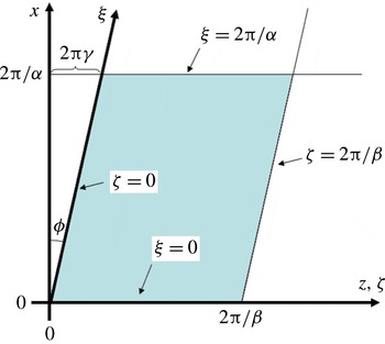
In oblique coordinates,
 $$\begin{eqnarray}\displaystyle {\it\xi}=x,\quad {\it\zeta}=-{\it\alpha}{\it\gamma}x+z, & & \displaystyle\end{eqnarray}$$
we apply periodic conditions of the form
 $$\begin{eqnarray}\displaystyle & [\boldsymbol{u},p]({\it\xi},y,{\it\zeta})=[\boldsymbol{u},p]({\it\xi}+2{\rm\pi}/{\it\alpha},y,{\it\zeta}), & \displaystyle\end{eqnarray}$$
 $$\begin{eqnarray}\displaystyle & [\boldsymbol{u},p]({\it\xi},y,{\it\zeta})=[\boldsymbol{u},p]({\it\xi},y,{\it\zeta}+2{\rm\pi}/{\it\beta}), & \displaystyle\end{eqnarray}$$
 ${\it\alpha}$
,
 ${\it\beta}$
and the tilt parameter
 ${\it\gamma}$
. The tilt angle of the domain is defined by
 ${\it\phi}=\arctan ({\it\alpha}{\it\gamma})$
. In the new coordinates the differential operators
 $\partial _{x}$
and
 $\partial _{z}$
in (2.1) must be replaced by
 $\partial _{{\it\xi}}-{\it\alpha}{\it\gamma}\partial _{{\it\zeta}}$
and
 $\partial _{{\it\zeta}}$
, respectively.
Schematic of the computational domain.

In order to solve the nonlinear equations, the Galerkin spectral code developed in Deguchi et al. (Reference Deguchi, Hall and Walton2013) for Cartesian coordinates is used as the basis of the numerical scheme. The code uses a toroidal–poloidal potential decomposition to simplify the problem. These potentials are first expanded by modified
 $l$
th-order Chebyshev polynomials in
 $y$
, and then each Chebyshev spectrum coefficient
 $a_{l}$
is further decomposed into Fourier series as
 $$\begin{eqnarray}\displaystyle a_{l}(x,z)=\mathop{\sum }_{m,n}\hat{a}_{lmn}\exp [\text{i}(m{\it\alpha}x+n{\it\beta}z)]+\text{c.c.}, & & \displaystyle\end{eqnarray}$$
where c.c. stands for complex conjugate. Instead of (2.4), following Deguchi & Altmeyer (Reference Deguchi and Altmeyer2013), here we use the expansion
 $$\begin{eqnarray}\displaystyle a_{l}({\it\xi},{\it\zeta})=\mathop{\sum }_{m,n}\hat{a}_{lmn}\exp [\text{i}(m{\it\alpha}-n{\it\alpha}{\it\beta}{\it\gamma})x+\text{i}n{\it\beta}z]+\text{c.c.} & & \displaystyle\end{eqnarray}$$
to compute solutions in a parallelogram-shaped domain. The algebraic equations for the unknown spectral coefficients resulting from a Galerkin projection are solved by using Newton’s method. The convergence criterion used here is the same as that used in Deguchi & Hall (Reference Deguchi and Hall2014a
). Note that the limit of
 ${\it\gamma}\rightarrow 0$
recovers the Cartesian case.
3. Numerical results and high-
 $Re$
asymptotic theories

In order to obtain solutions for
 ${\it\gamma}>0$
, we use a homotopy continuation of the solution branch from the mirror-symmetric solutions found by Gibson, Halcrow & Cvitanovic (Reference Gibson, Halcrow and Cvitanovic2009) and Itano & Generalis (Reference Itano and Generalis2009) for
 ${\it\gamma}=0$
. For wavenumbers
 $({\it\alpha},{\it\beta})=(0.75,1.37)$
, which we use throughout the paper, this solution arises as a saddle–node bifurcation at
 $Re\approx 140$
creating lower and upper branches; these branches are called EQ7 and EQ8 respectively in the latter paper. The solutions have symmetries
 $$\begin{eqnarray}\displaystyle & [u,v,w](x,y,z)=[u,v,-w](x+{\rm\pi}/{\it\alpha},y,-z), & \displaystyle\end{eqnarray}$$
 $$\begin{eqnarray}\displaystyle & [u,v,w](x,y,z)=[-u,-v,-w](-x,-y,-z), & \displaystyle\end{eqnarray}$$
 $$\begin{eqnarray}\displaystyle & [u,v,w](x,y,z)=[u,v,w](x+{\rm\pi}/{\it\alpha},y,z+{\rm\pi}/{\it\beta}). & \displaystyle\end{eqnarray}$$
 $w_{m}=\overline{w}$
, which is defined by the averaging operator
 $$\begin{eqnarray}\displaystyle \overline{\ast }=\frac{{\it\alpha}{\it\beta}}{4{\rm\pi}^{2}}\int _{0}^{2{\rm\pi}/{\it\alpha}}\int _{0}^{2{\rm\pi}/{\it\beta}}\ast \,\text{d}x\,\text{d}z. & & \displaystyle\end{eqnarray}$$
Also, we note that the solutions are steady, if they satisfy (3.1b ).
When
 ${\it\gamma}$
is increased from zero, any symmetry which involves reflection in
 $z$
is destroyed. This means that the shift–reflection symmetry (3.1a
) of the solution breaks and a spanwise mean flow must be produced. However, the symmetries (3.1b
) and (3.1c
) do not break, and thus the solution remains steady. Note that steady solutions with spanwise mean flow have already been reported in Gibson et al. (Reference Gibson, Halcrow and Cvitanovic2009). Those solutions, classified as EQ9–EQ13, also satisfy (3.1b
) but not (3.1a
) and (3.1c
).
The results obtained by gradually increasing
 ${\it\gamma}$
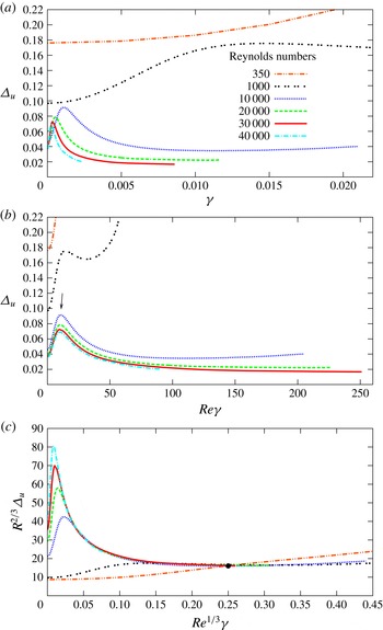
are shown in figure 2(a). The streamwise wall shear correction of the solution
 ${\it\Delta}_{u}=(\text{d}u_{m}/\text{d}y)|_{y=1}$
, defined by the streamwise mean flow correction
 $u_{m}=\overline{u}-y$
, is used as a measure of the solutions. The solution branches for
 $Re=350,1000,10\,000,20\,000,30\,000$
and 40 000 are shown in the figure. For relatively large
 $Re$
, first
 ${\it\Delta}_{u}$
increases when
 ${\it\gamma}$
is increased from zero and then reaches a maximum. The maximum points shift to smaller
 ${\it\gamma}$
with increasing
 $Re$
. The numerical results indicate that the value of
 ${\it\gamma}$
at the maximum scales like
 $Re^{-1}$
, as shown in figure 2(b); see the arrow in the figure which indicates the position of the maximum. After the maximum point,
 ${\it\Delta}_{u}$
decreases with increasing
 ${\it\gamma}$
. For large
 ${\it\gamma}$
a new scaling emerges: we find
 ${\it\gamma}\sim Re^{-1/3}$
,
 ${\it\Delta}_{u}\sim Re^{-2/3}$
which leads us to an asymptotic scaling valid even for
 $Re$
as low as 350; see figure 2(c). The following subsections describe these asymptotic behaviours using high-Reynolds-number asymptotic theories.
The change of the drag of the oblique exact coherent structures as a function of the tilt parameter for
 $({\it\alpha},{\it\beta})=(0.75,1.37)$
. To draw the diagrams, 100–110 Chebyshev modes are used in
 $y$
whilst 4–14 and 28–52 Fourier modes are used in
 ${\it\xi}$
and
 ${\it\zeta}$
, respectively. The arrow in (b) indicates the maximum of the drag.

3.1. The vortex–wave interaction stage
For
 ${\it\gamma}=0$
, Deguchi & Hall (Reference Deguchi and Hall2014b
) showed that with increasing
 $Re$
the lower branch mirror-symmetric mode solutions become vortex–wave interaction states, VWI for short. These states were derived by Hall & Smith (Reference Hall and Smith1991) and first applied to plane Couette flow by Hall & Sherwin (Reference Hall and Sherwin2010). The VWI theory has a deep relevance to the self-sustaining process picture of how exact coherent structures hold together. The self-sustaining process description was derived by Waleffe (Reference Waleffe1997) by a numerical interrogation of solutions of the Navier–Stokes equations. That interrogation showed how streamwise periodic waves occur as instabilities of a streak process but drive rolls through the Reynolds stress terms in the Navier–Stokes equations. The roll then drives the streak, thereby closing the process. In Hall & Smith (Reference Hall and Smith1991) the high-Reynolds-number description of that process had previously been explicitly derived in the context of boundary layer flows. Subsequently Hall & Sherwin (Reference Hall and Sherwin2010) showed, in the context of plane Couette flow, that the mechanism driving the rolls is essentially a steady streaming process involving a wave concentrated in its critical layer driving a streamwise-averaged flow. The self-sustained process picture was derived at finite Reynolds numbers and it is only because the VWI description turns out to apply at relatively low Reynolds number that the separation of individual processes was possible.
Following the VWI theory, now let us decompose the flow field into the vortex and wave components. The vortex component usually refers to the streamwise-averaged flow field, but here we define this component by averaging in
 ${\it\xi}$
and are concerned with how much we can increase the angle of this vortex component from the principal direction of the basic flow. Therefore, using the classical VWI scalings in Cartesian coordinates, we expand in the form
 $$\begin{eqnarray}\displaystyle & u=U+{\it\rho}(\tilde{u} \text{e}^{\text{i}{\it\alpha}{\it\xi}}+\text{c.c.})+\cdots \,, & \displaystyle\end{eqnarray}$$
 $$\begin{eqnarray}\displaystyle & v=Re^{-1}V+{\it\rho}(\tilde{v}\text{e}^{\text{i}{\it\alpha}{\it\xi}}+\text{c.c.})+\cdots \,, & \displaystyle\end{eqnarray}$$
 $$\begin{eqnarray}\displaystyle & w=Re^{-1}W+{\it\rho}(\tilde{w}\text{e}^{\text{i}{\it\alpha}{\it\xi}}+\text{c.c.})+\cdots \,, & \displaystyle\end{eqnarray}$$
 $$\begin{eqnarray}\displaystyle & p=Re^{-2}P+{\it\rho}(\tilde{p}\text{e}^{\text{i}{\it\alpha}{\it\xi}}+\text{c.c.})+\cdots \,, & \displaystyle\end{eqnarray}$$
 $[U,V,W,P](y,{\it\zeta})\in \mathbb{R}$
and
 $[\tilde{u} ,\tilde{v},\tilde{w},\tilde{p}](y,{\it\zeta})\in \mathbb{C}$
are the vortex and wave components, respectively. Hereafter we refer to
 $U$
and
 $(V,W)$
as streak and roll, respectively. The scaling for the roll–streak components follows from the usual Taylor-vortex scaling that allows the viscous effect to be present in the whole channel; see Taylor (Reference Taylor1923) for example. On top of the roll–streak a wave of unknown amplitude propagates. The size of the wave,
 ${\it\rho}\ll Re^{-1}$
, is to be fixed in terms of
 $Re$
so that it drives the vortex by inducing a stress jump across the critical layer.
The leading-order equations for the vortex component are
 $$\begin{eqnarray}\displaystyle & [V\partial _{y}+(W-{\it\alpha}{\it\gamma}_{0}U)\partial _{{\it\zeta}}]\left[\begin{array}{@{}c@{}}U\\ V\\ W\end{array}\right]=-\!\left[\begin{array}{@{}c@{}}0\\ \partial _{y}P\\ \partial _{{\it\zeta}}P\end{array}\right]+[\partial _{y}^{2}+\partial _{{\it\zeta}}^{2}]\left[\begin{array}{@{}c@{}}U\\ V\\ W\end{array}\right]\!, & \displaystyle\end{eqnarray}$$
 $$\begin{eqnarray}\displaystyle & \partial _{y}V+\partial _{{\it\zeta}}(W-{\it\alpha}{\it\gamma}_{0}U)=0, & \displaystyle\end{eqnarray}$$
 ${\it\gamma}=Re^{-1}{\it\gamma}_{0}$
to remove
 $Re$
from the equations. The
 $Re^{-1}$
scaling of
 ${\it\gamma}$
follows from the relative size of the roll and streak. The scaling determines an appropriate angle between the directions of the basic flow and the viscous roll–streak, and has a close relationship to the work of Hall (Reference Hall1985) on the Görtler vortex problem in three-dimensional boundary layers.
The leading-order wave equations satisfy the inviscid equations linearized around the streaky field
 $[U,0,0]$
that can be transformed into a generalized Rayleigh equation:
 $$\begin{eqnarray}\left(\partial _{y}^{2}+\partial _{{\it\zeta}}^{2}-{\it\alpha}^{2}-2\frac{\partial _{y}U}{U}\partial _{y}-2\frac{\partial _{{\it\zeta}}U}{U}\partial _{{\it\zeta}}\right)\tilde{p}=0.\end{eqnarray}$$
The Rayleigh equation (3.5) is singular at the critical layer
 $y=f({\it\zeta})$
where
 $U(f({\it\zeta}),{\it\zeta})=0$
so we need a separate analysis there. In order to regularize the equation we need to bring back viscosity and the viscous–convective balance gives the classical critical layer thickness
 ${\it\delta}_{c}=Re^{-1/3}$
. From the local expansion around the critical layer the wave velocity component tangential to the critical layer, say
 $\tilde{v}^{s}$
, must increase by a factor of
 ${\it\delta}_{c}^{-1}$
. Then the wave creates a Reynolds stress in the critical layer which balances the viscous term in the vortex system. Integrating the vortex equations across the critical layer, we can find that the stress jump drives the roll flow. The unknown wave size
 ${\it\rho}$
is then fixed by making that jump of
 $O((Re\tilde{v}^{s})^{2}{\it\delta}_{c})$
, comparable to the
 $O(1)$
roll stresses outside of the critical layer. From that balance we deduce
 ${\it\rho}=Re^{-7/6}$
.
The critical layer equations derived in this way are exactly the same as the Cartesian case on replacing
 $(x,y)$
by
 $({\it\xi},{\it\zeta})$
. Therefore, as shown in Hall & Sherwin (Reference Hall and Sherwin2010), switching from
 $(y,{\it\zeta})$
to the body-fitted coordinates (
 $n$
,
 $s$
), where
 $n$
and
 $s$
represent the normal and tangential coordinates along the critical layer, the stress jump of the roll component can be analytically solved as
 $$\begin{eqnarray}\displaystyle & [\partial _{n}V^{s}]_{-}^{+}=n_{0}{\it\alpha}^{-5/3}\partial _{s}({\it\mu}^{-5/3}|\partial _{s}\tilde{p}|^{2}), & \displaystyle\end{eqnarray}$$
 $$\begin{eqnarray}\displaystyle & [P]_{-}^{+}=-n_{0}({\it\alpha}{\it\mu})^{-5/3}{\it\Lambda}_{0}|\partial _{s}\tilde{p}|^{2}, & \displaystyle\end{eqnarray}$$
 $V^{s}(n,s)$
is the roll velocity tangential to the critical layer,
 ${\it\mu}=(\partial _{n}U)|_{y=f}$
is the streak shear evaluated on the critical layer,
 ${\it\Lambda}_{0}$
is the critical layer curvature, and
 $n_{0}=2{\rm\pi}(2/3)^{2/3}{\it\Gamma}(1/3)$
. The jump closes the problem and (3.4)–(3.6) constitute a self-consistent set of equations formally derived from the Navier–Stokes equations in the limit
 $Re\rightarrow \infty$
.
The above discussion clearly shows that the VWI theory is still valid for
 ${\it\gamma}\sim O(Re^{-1})$
, consistent with figure 2(b). The overall interaction scenario does not change from the usual VWI; the tilt angle just controls the vortex advection by the streak field in (3.4), and does not influence the structure of the wave system (3.5) and the jump conditions (3.6). In this VWI regime, the streamwise wall shear correction
 ${\it\Delta}_{u}$
is
 $O(1)$
whilst the spanwise wall shear
 ${\it\Delta}_{w}$
, defined by
 $(\text{d}w_{m}/\text{d}y)|_{y=1}$
, is
 $O(Re^{-1})$
. Note that our result here also supports the conclusion by Deguchi & Hall (Reference Deguchi and Hall2014b
) that the large-Reynolds-number mirror-symmetric mode is of VWI type.
3.2. The boundary region equations
In the last subsection we saw that when
 ${\it\gamma}$
becomes larger than
 $O(Re^{-1})$
the VWI structure breaks down. The breakdown process, which we shall concentrate on here, is similar to that observed in Deguchi et al. (Reference Deguchi, Hall and Walton2013), where a long streamwise wavelength of
 $O(Re)$
is considered. The key point of the theory is that the critical layer spreads out to fill the whole channel so that we have a regular behaviour everywhere in the flow. The outcome of the spreading is that the vortex and wave components are comparable in size and it is not possible to distinguish between these quantities. In Deguchi et al. (Reference Deguchi, Hall and Walton2013), the long-wavelength asymptotic states were found to be governed by the so-called boundary-region equations (BREs), instead of the VWI system (3.4)–(3.6). The BREs are given by (2.1a
) and (2.1b
) with unit
 $Re$
and
 $\partial _{x}$
neglected on the right-hand side of (2.1a
). However, because now we fix the streamwise wavelength to be of
 $O(1)$
, there are several fundamental differences.
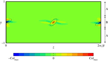
The streamwise vorticity
 ${\it\omega}=(\partial _{z}v-\partial _{y}w)$
of the nonlinear solutions at
 $x=0$
for
 $({\it\alpha},{\it\beta},{\it\gamma})=(0.75,1.37,0.25Re^{-1/3})$
. Colour represents the localization of flow structure at the filled circle in figure 2(c) where
 $Re=30\,000$
and
 $\text{Col}_{max}=0.0849$
. The three ovals placed at each localized structure represent 60 % maximum of
 $|{\it\omega}|$
for
 $Re=1000,10\,000$
and 30 000, from outside to inside.

In order to find the asymptotic structure observed in figure 2(c), we first examine the numerically obtained flow properties. Figure 3 shows the streamwise vorticity
 ${\it\omega}$
of the oblique exact coherent states for
 ${\it\gamma}=0.25Re^{-1/3}$
in a
 $y$
–
 $z$
cross-section at
 $x=0$
. The colour in the figure shows that the vortex structure is localized in
 $y$
, similar to the unbounded VWI. Moreover, the structure is also localized in
 $z$
; in fact, the tails of the localized structure exponentially decay as observed by Gibson & Brand (Reference Gibson and Brand2014). We observe that the localized structure shrinks in both
 $y$
and
 $z$
with increasing
 $Re$
. Two families of three superimposed ovals in the figure are 60 % maximum of
 $|{\it\omega}|$
for
 $Re=1000,10\,000$
and 30 000. This property highlights a physical difference from the VWI case where roll–streak components occupy the whole channel. Also, in contrast to VWI, the states governed by BREs could possess a complicated streamwise dependence; recall that the streamwise dependence of the VWI states is dominated by a monochromatic Rayleigh neutral wave. Detailed visualizations of the VWI states can be found in Hall & Sherwin (Reference Hall and Sherwin2010), Blackburn et al. (Reference Blackburn, Hall and Sherwin2013) and Deguchi & Hall (Reference Deguchi and Hall2014a
,Reference Deguchi and Hall
b
).
In view of the observation above we scale
 $(y,{\it\zeta})$
as
 $y={\it\epsilon}Y$
and
 ${\it\zeta}={\it\epsilon}Z$
with a small parameter
 ${\it\epsilon}$
to be specified later. We then expand the flow field as
 $$\begin{eqnarray}\displaystyle & u=Re^{-1}{\it\epsilon}^{-2}U({\it\xi},Y,Z)+Re^{-1}{\it\epsilon}^{-1}U_{1}({\it\xi},Y)+Re^{-1}d_{u}Y+\cdots \,, & \displaystyle\end{eqnarray}$$
 $$\begin{eqnarray}\displaystyle & v=Re^{-1}{\it\epsilon}^{-1}V({\it\xi},Y,Z)+Re^{-1}V_{1}({\it\xi},Y)+\cdots \,, & \displaystyle\end{eqnarray}$$
 $$\begin{eqnarray}\displaystyle & w=Re^{-1}{\it\epsilon}^{-1}W({\it\xi},Y,Z)+Re^{-1}W_{1}({\it\xi},Y)+{\it\epsilon}Re^{-1}d_{w}Y+\cdots \,, & \displaystyle\end{eqnarray}$$
 $$\begin{eqnarray}\displaystyle & p=Re^{-2}{\it\epsilon}^{-2}P({\it\xi},Y,Z)+Re^{-2}{\it\epsilon}^{-1}P_{1}({\it\xi},Y)+\cdots \,, & \displaystyle\end{eqnarray}$$
 $O({\it\epsilon})$
, i.e. the layer ‘B’ in figure 3. The size of the leading-order spanwise-averaged disturbance component, denoted by subscript 1, must be
 ${\it\epsilon}$
times smaller than the other leading-order terms, because the Reynolds stress driving this component is
 $O({\it\epsilon})$
times smaller than that for the other component due to the spanwise localization. Therefore the spanwise average of
 $[U,V,W]$
must be the ‘basic’ flow
 $[Y,0,0]$
. The constants
 $d_{u}$
and
 $d_{w}$
appearing in the smaller-order terms are to be determined by the second-order spanwise-averaged flow problem. Substituting the above expansions into the scaled Navier–Stokes equations, we obtain a modified form of the BREs to leading order:
 $$\begin{eqnarray}\displaystyle & [U\partial _{{\it\xi}}+V\partial _{Y}+(W-{\it\alpha}{\it\gamma}_{0}U)\partial _{Z}]\left[\begin{array}{@{}c@{}}U\\ V\\ W\end{array}\right]=-\!\left[\begin{array}{@{}c@{}}0\\ \partial _{Y}P\\ \partial _{Z}P\end{array}\right]+[\partial _{Y}^{2}+\partial _{Z}^{2}]\left[\begin{array}{@{}c@{}}U\\ V\\ W\end{array}\right]\!, & \displaystyle\end{eqnarray}$$
 $$\begin{eqnarray}\displaystyle & \partial _{{\it\xi}}U+\partial _{Y}V+\partial _{Z}(W-{\it\alpha}{\it\gamma}_{0}U)=0, & \displaystyle\end{eqnarray}$$
 $$\begin{eqnarray}\displaystyle & [U,V,W]\rightarrow [Y,0,0]\quad \text{as }Y\rightarrow \pm \infty , & \displaystyle\end{eqnarray}$$
 ${\it\gamma}={\it\epsilon}{\it\gamma}_{0}$
in order to balance the effect of the inclination of the domain. Equations (3.8) must be solved with periodic conditions in
 ${\it\xi}$
and exponentially decaying conditions in
 $Z$
for the disturbance. Thus we do not need to consider the spanwise-averaged part of these leading-order equations. This is the first difference from Deguchi et al. (Reference Deguchi, Hall and Walton2013), where the periodic condition is considered in the asymptotic problem, although they reported spanwise localized numerical solutions. The second difference is in the boundary conditions in
 $Y$
that imply we are seeking a solution in an unbounded domain such as the unbounded VWI problem formulated by Blackburn et al. (Reference Blackburn, Hall and Sherwin2013) and Deguchi & Hall (Reference Deguchi and Hall2014b
). The origin of the vertical localization is that we need a short vertical length scale to recover the regularity of the wave equation when the streamwise wavelength is restricted to be of
 $O(1)$
. Outside of the interaction layer, the regions ‘A’ in figure 3, all of the disturbances decay except for the mean flow corrections which must take the form of an unforced linear profile. Since
 $U$
matches to the basic flow component
 $y$
at large
 $|Y|$
, we require
 $Re^{-1}{\it\epsilon}^{-2}Y=y={\it\epsilon}Y$
, i.e.
 ${\it\epsilon}=Re^{-1/3}$
.
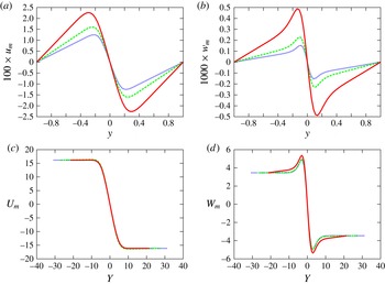
The mean flow correction of the nonlinear Navier–Stokes solutions for
 $({\it\alpha},{\it\beta},{\it\gamma})=(0.75,1.37,0.25Re^{-1/3})$
: (a,b) non-scaled quantities
 $u_{m}$
and
 $w_{m}$
; (c,d) scaled quantities
 $U_{m}=Re^{2/3}u_{m}-Re^{-1/3}d_{u}Y$
and
 $W_{m}=Rew_{m}-Re^{-1/3}d_{w}Y$
in the expansion (3.7), where displacement velocities are
 $d_{u}=16.16$
and
 $d_{w}=3.456$
. Red solid, green dashed and blue dotted lines are for
 $Re=10\,000$
, 20 000 and 30 000, respectively.

The components
 $[U_{1},V_{1},W_{1}]$
and
 $P_{1}$
are determined by the spanwise-averaged equations
 $$\begin{eqnarray}\displaystyle \langle VU\rangle =\partial _{Y}^{2}U_{1},\quad \langle V^{2}\rangle =-\partial _{Y}P_{1}+\partial _{Y}^{2}V_{1}, & & \displaystyle\end{eqnarray}$$
 $$\begin{eqnarray}\displaystyle \langle VW\rangle =\partial _{Y}^{2}W_{1},\quad \partial _{{\it\xi}}U_{1}+\partial _{Y}V_{1}=0, & & \displaystyle\end{eqnarray}$$
 $$\begin{eqnarray}\displaystyle [U_{1},V_{1},W_{1}]\rightarrow [\mp d_{u},0,\mp d_{w}]\quad \text{as }Y\rightarrow \pm \infty , & & \displaystyle\end{eqnarray}$$
where
 $\langle \ast \rangle =\lim _{L\rightarrow \infty }(1/L)\int _{0}^{L}\ast \,\text{d}Z$
. The constants
 $d_{u}$
and
 $d_{w}$
are the displacement velocities in the mean flows
 $U_{m}(Y)=\overline{U}_{1}$
and
 $W_{m}(Y)=\overline{W}_{1}$
produced as a result of nonlinear interactions. These components, and smaller linear terms
 $Re^{-1}d_{u}$
and
 ${\it\epsilon}Re^{-1}d_{w}$
in (3.7), match to the unforced mean flow corrections of the linear profile outside of the interaction layer. The matching process is similar to that found in Deguchi & Hall (Reference Deguchi and Hall2014b
). Since the mean flow corrections must be written in the form of
 $u_{m}\approx {\it\Delta}_{u}(y\mp 1)$
and
 $w_{m}\approx {\it\Delta}_{w}(y\mp 1)$
in the region ‘A’, the matching conditions yield
 $u_{m}=Re^{-1}{\it\epsilon}^{-1}d_{u}(y\mp 1)$
and
 $w_{m}=Re^{-1}d_{w}(y\mp 1)$
. Therefore, the wall shears and displacement velocities are
 ${\it\Delta}_{u}=Re^{-2/3}d_{u}$
and
 ${\it\Delta}_{w}=Re^{-1}d_{w}$
.
In order to confirm the asymptotic structure, we plot the streamwise and spanwise mean flow corrections from the full Navier–Stokes calculation for
 $Re=10\,000,20\,000$
and 30 000 in figure 4(a,b). When we apply the scaling
 $U_{m}=Re^{2/3}u_{m}-Re^{-1/3}d_{u}Y$
and
 $W_{m}=Rew_{m}-Re^{-1/3}d_{w}Y$
to the mean flows, as shown in figure 4(c,d), the scaled mean flows converge to a single curve with increasing
 $Re$
. Consistent with the theory, for large
 $|Y|$
the streamwise and spanwise scaled mean flows become the constant displacement velocities,
 $\pm d_{u}=16.16$
and
 $\pm d_{w}=3.456$
, respectively, calculated by the wall shears.
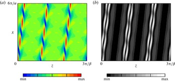
The asymptotically converged solution scaled for
 $Re=350$
. The solution shown in figure 3 is used for the asymptotic extrapolation. (a) Streamwise vorticity at
 $y=0$
, (b) kinetic energy
 $(u^{2}+v^{2}+w^{2})/2$
at
 $y=0$
.

We recall that the BREs scaling in figure 2(c) gives a better agreement of the
 $Re=350$
curve with the asymptotically converged large-
 $Re$
results compared with figure 2(a,b). Thus for relatively small
 $Re$
it would be sensible to use BREs to describe oblique patterns. If the solution obtained for
 $Re=30\,000$
is considered to be a good approximation to the solution of the reduced problem (3.8), we can use it to predict the behaviour of the oblique exact coherent structures for various values of
 $Re$
. For definiteness, here we consider such a prediction for
 $Re=350$
to compare with the simulation by Barkley & Tuckerman (Reference Barkley and Tuckerman2005). By increasing the tilt angle by a factor of
 $(30\,000/350)^{1/3}$
and extending the flow regime in the spanwise direction by the same factor as from the solution shown in figure 3, we have a prediction for the vorticity distribution at the mid-channel as shown in figure 5(a). In the figure, we can clearly see an oblique band structure localized in the spanwise direction.
The corresponding kinetic energy at the mid-plane of this regime is presented in figure 5(b). The region where the energy is highest is visualized by the small bright blobs aligned in oblique fashion and is seen to be similar to those observed in figures 1 and 5 of Barkley & Tuckerman (Reference Barkley and Tuckerman2005). However, in the simulation many blobs are clustered to create a large-scale laminar–turbulent band structure, whilst in our case the oblique band is created by a single line of localized blobs. This means that further computations are required before we reach a definitive conclusion. Here we remark that the difference could be resolved if we assume that the asymptotic equations can support more complicated asymptotic solutions which play a more important role in the dynamics. Thus one of the possible scenarios would be for the reduced system (3.8) to have solutions with clustered blobs connected by snakings of the solution branch similar to Schneider, Gibson & Burke (Reference Schneider, Gibson and Burke2010) or Deguchi & Hall (Reference Deguchi and Hall2014a ). Alternatively a direct comparison with numerical simulations for various Reynolds numbers could be used to validate our theory. Also, notice that the difference of the shape of the domains is not a significant issue in the comparison because the domains used both in this work and in Barkley & Tuckerman (Reference Barkley and Tuckerman2005) are appropriate periodic boxes to describe the minimum structure of the banded patterns, which are self-organized in large computational domains.
Once we have the solution of (3.8) for some
 ${\it\alpha}$
, an asymptotic solution with a different value of wavenumber, say
 $\hat{{\it\alpha}}$
, can be easily obtained following a self-similar transformation similar to that proposed for unbounded VWI by Blackburn et al. (Reference Blackburn, Hall and Sherwin2013):
 $$\begin{eqnarray}U=a^{1/3}\hat{U} ,\quad V=a^{-1/3}\hat{V},\quad W=a^{-1/3}{\hat{W}},\quad P=a^{-2/3}\hat{P},\end{eqnarray}$$
 $$\begin{eqnarray}{\it\xi}=a\hat{{\it\xi}},\quad Y=a^{1/3}{\hat{Y}},\quad Z=a^{1/3}\hat{Z},\quad {\it\gamma}_{0}=a^{1/3}\hat{{\it\gamma}}_{0},\end{eqnarray}$$
where
 $a=\hat{{\it\alpha}}/{\it\alpha}$
. It is easy to confirm that the hat variables satisfy the same problem as (3.8) with a wavenumber
 $\hat{{\it\alpha}}$
in
 $\hat{{\it\xi}}$
. We can increase the value of
 $a$
until the nonlinear interaction layer of depth
 ${\it\delta}=O(a^{1/3}Re^{-1/3})$
fills the entire gap. For maximum
 $a\sim O(Re)$
, the streamwise wavenumber is
 ${\it\alpha}\sim O(Re^{-1})$
and the same long-wavelength problem as discussed in Deguchi et al. (Reference Deguchi, Hall and Walton2013) is recovered if
 $\hat{{\it\gamma}}_{0}=0$
. The tilt angle predicted for this largest-scale case, where the kinetic energy at the mid-plane is the most significant, is
 $\tan {\it\phi}={\it\alpha}{\it\gamma}\sim O({\it\alpha}^{2/3}Re^{-1/3})\sim O(Re^{-1})$
.
4. Conclusion
We have continued the solution branch of the mirror-symmetric exact coherent states in plane Couette flow to parallelogram-shaped computational domains. When the tilt angle of the domain
 ${\it\phi}$
is increased, we find that the solution develops into an oblique banded pattern. Our results for large
 $Re$
were used to motivate asymptotic analyses which explained the parameter dependence of the results.
For small
 ${\it\phi}$
the oblique exact coherent states first obey the modified VWI theory satisfying
 $\tan {\it\phi}\sim O(Re^{-1})$
scaling. The scaling, obtained by considering the advection balance due to the roll and streak components, is consistent with Barkley & Tuckerman (Reference Barkley and Tuckerman2007), where the oblique banded pattern observed in the experiments and simulations is summarized. Good convergence of the numerical solutions to this asymptotic result are observed for relatively large
 $Re$
of
 $O(10^{4})$
.
When the tilt angle of the domain is further increased, the solution eventually develops a localized structure in both spanwise and wall-normal directions. A new asymptotic theory was developed for this regime and it is found that the centre of the nonlinear interaction at the localized position is governed by the modified boundary-region equations. That situation is similar to the long-wavelength VWI theory by Deguchi et al. (Reference Deguchi, Hall and Walton2013); however, here we found that the nonlinear interaction only occurs in a region of vertical and spanwise length scales of
 $O(({\it\alpha}Re)^{-1/3})$
, where
 ${\it\alpha}$
is the streamwise wavenumber. The localization of the nonlinear structure naturally creates a laminar–turbulent banded pattern. The new theory has two important properties: (i) the local nonlinear structure can be embedded in any shear flow when the basic flow is locally approximated by a linear profile; (ii) the local nonlinear structure is invariant under certain self-similar transformation, and therefore the theory can be applicable for various spatial scales. These properties are similar to those seen in the VWI theory in an unbounded domain.
The theoretical tilt angle for the BREs state is
 $\tan {\it\phi}\sim O({\it\alpha}{\it\delta})$
, where
 ${\it\delta}\sim ({\it\alpha}Re)^{-1/3}$
. For the largest-scale structure, which is the most energetic and has
 ${\it\alpha}\sim O(Re^{-1})$
and
 ${\it\delta}\sim O(1)$
, the scaling of the tilt angle is again consistent with Barkley & Tuckerman (Reference Barkley and Tuckerman2007). Our numerical computations suggest that the asymptotically converged result can at least qualitatively predict the oblique exact coherent structures even for transitional
 $Re$
as low as
 $350$
, which is used in the simulation by Barkley & Tuckerman (Reference Barkley and Tuckerman2005). The appropriately rescaled asymptotic results for
 $Re=350$
are at least qualitatively reminiscent of the simulation. Therefore the essential sustainment mechanism behind the oblique banded pattern in subcritical shear flows is likely to be elucidated by the BRE-type asymptotic theory developed in this paper.
Acknowledgements
This work was supported by EPSRC grant EP/1037946/1. The authors would like to thank the referees for their helpful comments.