


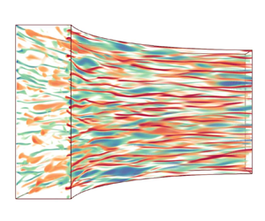



1. Introduction
Taylor–Couette flow (TCF), i.e. fluid flow enclosed by two coaxial and independently rotating cylinders, is a paradigm for studies of flow instability and turbulence dynamics, owing to its geometric simplicity and versatility in generating diverse flow regimes (Grossmann, Lohse & Sun Reference Grossmann, Lohse and Sun2016). Specifically, TCF exhibits a rich phase diagram. For example, inner-cylinder-rotating-only (ICRO) TCF exhibits supercritical centrifugal instability, while turbulence arises in strong counter-rotating TCF via a subcritical shear instability. Recently, in co-rotating TCF a subtle regime known as Keplerian flow has gained increasing attention, due to its fundamental importance to relevant astrophysics (Ji & Goodman Reference Ji and Goodman2023). This flow regime is centrifugally stable and is characterized by the angular velocity ratio  $\omega _{o}/\omega _{i}=(r_{o}/r_{i})^{p}$ with
 $p=-3/2$, where
 $r_{i,o}$ are the radii of the inner and outer cylinders and
 $\omega _{i,o}$ their angular velocities, respectively. Thus, the existence of turbulence in Keplerian flows and the corresponding mechanism of angular momentum transport is of great interest. Although subcritically unstable shear flows become turbulent when the shear Reynolds number (
 $Re$) is sufficiently large, there is no concrete evidence that hydrodynamic instability alone can sustain turbulence in the Keplerian regime. Unfortunately, experiments in TCF are difficult to conduct and interpret in this regime due to major axial end cap effects that could cause secondary flows and influence the global stability of the flow (Avila Reference Avila2012; Lopez & Avila Reference Lopez and Avila2017). In fact, when one minimizes the end effect to the extent possible, turbulence does not arise in TCF experiments up to
 $Re=2\times 10^6$ (Ji et al. Reference Ji, Burin, Schartman and Goodman2006; Schartman et al. Reference Schartman, Ji, Burin and Goodman2012). Moreover, direct numerical simulations (DNS) with axial periodicity either with centrifugally driven turbulence as an initial condition (Ostilla-Mónico et al. Reference Ostilla-Mónico, Verzicco, Grossmann and Lohse2014) or after the introduction of an optimal perturbation for transient growth (Shi et al. Reference Shi, Hof, Rampp and Avila2017) exhibit turbulence decay in the Keplerian regime.
In contrast to the increased interest in the Keplerian regime of Newtonian TCF, its non-Newtonian counterpart continues to not attract much attention, despite the fact that the so-called elastorotational instability (ERI) in the Keplerian regime is regarded as a close analogue of turbulence in astrophysical accretion disks that arises due to a magnetorotational instability (MRI) (Ogilvie & Proctor Reference Ogilvie and Proctor2003; Ogilvie & Potter Reference Ogilvie and Potter2008). This analogy relies on a rigorous theoretical foundation that the viscoelastic stresses in dilute polymeric fluids, which follow a dumbbell model, and the Maxwell stresses in electric conducting fluids, which follow the magnetohydrodynamics (MHD) equation, have mathematically similar terms (Vieu & Mutabazi Reference Vieu and Mutabazi2019). Hence, the physical mechanisms that destabilize a viscoelastic flow are remarkably similar to the MRI (Boldyrev, Huynh & Pariev Reference Boldyrev, Huynh and Pariev2009; Dey et al. Reference Dey, Chatterjee, Murthy, Korsós, Liu, Nelson and Erdélyi2022). Therefore, experimental studies and simulations of ERI in the Keplerian regime are of great interest, as laboratory demonstrations of MRI have proved difficult due to the fact that to trigger MRI, even for the most highly conducting liquid metals, one must reach  $Re$ in excess of
 $10^6$. Specifically, in recent years Bai, Crumeyrolle & Mutabazi (Reference Bai, Crumeyrolle and Mutabazi2015) have identified four different modes in viscoelastic TCF experiments in the Keplerian regime, namely, a stationary axisymmetric mode composed of vortices with an axial wavelength smaller than the gap width, a disordered wave mode, a solitary vortex mode and a pure elasticity mode. Interestingly, the first three modes cease to exist in the anti-Keplerian regime (
 $\,p=3/2$), so they are ERI modes which are analogous to MRI (Ogilvie & Potter Reference Ogilvie and Potter2008; Boldyrev et al. Reference Boldyrev, Huynh and Pariev2009; Bai et al. Reference Bai, Vieu, Crumeyrolle and Mutabazi2021). As expected, the purely elastic mode arises regardless of rotating conditions (Larson, Shaqfeh & Muller Reference Larson, Shaqfeh and Muller1990). Experimental evidence to date suggests that sufficiently large shear and elastic energies are a prerequisite for triggering ERI modes. However, the aforementioned experimental observations and theoretical analysis of ERI are of limited use due to their small
 $Re$ (
 ${<}100$), which are close to the onset condition for ERI. In fact, as suggested by Ogilvie & Potter (Reference Ogilvie and Potter2008), the analogy between viscoelastic and MHD flows is more accurate at large values of
 $Re$. In this respect, the ERI-induced turbulence would be analogous to a turbulent accretion disk containing a magnetic field. This analogy is of great interest as it allows examination of the turbulent regime of viscoelastic TCF with Keplerian rotation.
Hence, we conduct DNS of Keplerian turbulence, namely, the turbulent state with Keplerian rotation, in TCF of dilute polymeric solutions up to  $Re=10^4$. Polymer additives can induce turbulence in Keplerian flow realized in axially periodic TCF via the ERI. We closely examine the coherent flow structures in this novel turbulent flow state and reveal a scaling law between angular momentum transport and the driving force. Furthermore, we analytically derive the exact relation between energy dissipation and angular momentum transport, which demonstrates that the combination of Newtonian and polymeric effects results in the observed scaling law.
2. Numerical details
We explore Keplerian turbulence in TCF of dilute polymeric solutions by DNS via a high-fidelity robust and efficient finite-difference algorithm that has proven successful in simulating inertially to elastically dominated turbulent flows (Lin et al. Reference Lin, Wan, Zhu, Liu, Lu and Khomami2022). We have chosen  $d=r_o-r_i$,
 $U=r_i|\omega _i-\omega _o|$,
 $d/U$ and
 $\rho U^2$ as scales for length, velocity
 $\boldsymbol {u}$, time and pressure
 $P$, respectively. Here,
 $\rho$ denotes the solution density and
 $\boldsymbol{u}$ consists of three components
 $(u_r, u_\theta, u_z)$ corresponding in sequence to the cylindrical coordinates
 $(r, \theta, z)$. The polymer stress
 $\boldsymbol {\tau }$ is related to the conformation tensor
 $\boldsymbol{\mathsf{C}}$ through the FENE-P (finitely extensible nonlinear elastic-Peterlin) model. To capture the shear and rotation effects, we perform simulations in a frame of reference that co-rotates with the outer cylinder. The dimensionless governing equations are
 $$\begin{gather} \boldsymbol{\nabla}\boldsymbol{\cdot}\boldsymbol{u} = 0, \end{gather}$$
 $$\begin{gather}\frac{\partial \boldsymbol{u}}{\partial t}+\boldsymbol{u}\boldsymbol{\cdot} \boldsymbol{\nabla} \boldsymbol{u}=-\boldsymbol{\nabla} P+\frac{\beta}{Re}\nabla^2\boldsymbol{u}+\frac{1-\beta}{Re}\boldsymbol{\nabla} \boldsymbol{\cdot} \boldsymbol{\tau}-Ro^{-1}\boldsymbol{e}_{z}\times \boldsymbol{u} \end{gather}$$
and
 \begin{equation} \frac{\partial \boldsymbol{\mathsf{C}}}{\partial t}+\boldsymbol{u} \boldsymbol{\cdot} \boldsymbol{\nabla}\boldsymbol{\mathsf{C}}=\boldsymbol{\mathsf{C}}\boldsymbol{\cdot} \boldsymbol{\nabla} \boldsymbol{u}+(\boldsymbol{\nabla} \boldsymbol{u})^{\rm T}\boldsymbol{\cdot} \boldsymbol{\mathsf{C}}-\boldsymbol{\tau}, \end{equation}
where  $\beta =\eta _s/\eta _t$ is the viscosity ratio between the solvent viscosity
 $\eta_s$ and the viscosity of the solution at zero shear rate,
 $\eta_t$, and
 $Re=\rho U d/\eta _t$ is the shear Reynolds number based on the azimuthal velocity of the inner cylinder in the rotating frame. The effect of outer cylinder rotation is manifested in a Coriolis force
 $Ro^{-1}\boldsymbol {e}_{z}\times \boldsymbol {u}$, where
 $Ro=U/(2\omega _o d)$ is the Rossby number and
 $e_z$ is the unit vector in the axial direction (Ostilla-Mónico et al. Reference Ostilla-Mónico, Verzicco, Grossmann and Lohse2014). Moreover, the polymer stress
 $\boldsymbol {\tau }$ is related to the conformation tensor via the relationship
 $\boldsymbol {\tau }=(\,f(\boldsymbol{\mathsf{C}})\boldsymbol{\mathsf{C}}-\boldsymbol{\mathsf{I}})/Wi$, where
 $f(\boldsymbol{\mathsf{C}})=(L^2-3)/(L^2-\text {trace}(\boldsymbol{\mathsf{C}}))$ is the Peterlin function,
 $\boldsymbol{\mathsf{I}}$ is the unit tensor and
 $Wi=\lambda U/d$ is the Weissenberg number, with
 $\lambda$ and
 $L$ being the polymer relaxation time and the maximum chain length, respectively. The governing equations are supplemented with no-slip boundary conditions at walls, as well as periodic boundary conditions in the axial direction.
We performed simulations at a radius ratio of  $\eta =r_i/r_o=0.8$, which leads to
 $Ro^{-1}\approx 1.2577$ for the Keplerian regime
 $\omega _o/\omega _i=\eta ^{3/2}$. The fluid confined between the two concentric cylinders is a dilute polymeric solution composed of long linear polymer chains with
 $\beta =0.9$ and
 $L=100$. To extensively explore the flow dynamics, including the scaling feature in the Keplerian regime, simulations over a broad range of
 $Re$ are carried out: specifically,
 $Re$ is increased over two decades from
 $10^2$ to
 $10^4$, corresponding to an elasticity number (
 $El=Wi/Re$) range of
 $3\times 10^{-3} \sim 0.3$ at a selected
 $Wi=30$. According to Bai et al. (Reference Bai, Crumeyrolle and Mutabazi2015), the critical modes observed for
 $El < El_{0}$ arise due to ERI, where
 $El_{0}$ represents the transition threshold from ERI to purely elastic instability;
 $El_{0} =0.672$ for
 $\eta =0.8$. Hence, ERI that signifies the combination of elastic and rotational effects should destabilize the flow under consideration. Table 1 contains the details of the grid resolutions at various
 $Re$. To strike a balance between flow resolution accuracy and computational efficiency, we gradually refine the grids with the increase of
 $Re$. Moreover, we cluster grid points near the cylinder walls to accurately capture the localized flow structures. The low values of
 $\varDelta _{\epsilon }$ for all
 $Re$ demonstrate the adequacy of grids used in the simulations. Specifically, Ostilla-Mónico et al. (Reference Ostilla-Mónico, Stevens, Grossmann, Verzicco and Lohse2013) have shown that a value of less than
 $1\,\%$ for
 $\varDelta _{\epsilon }$ leads to reliable results at the simulated
 $Re$. The time step is varied between
 $4\times 10^{-3}$ and
 $1\times 10^{-3}$ depending on the flow conditions. To obtain statistically stationary flow states, we perform long simulations typically of 500
 $T$, where
 $T=d/U$ is the convective time unit. Moreover, we use ensemble averaging for time periods of at least
 $500T$ to evaluate the turbulence statistics.
Grid resolutions for different cases, with  $N_r$,
 $N_\theta$ and
 $N_z$ being the numbers of grid points in the radial, azimuthal and axial directions, respectively. Here,
 $L_z$ represents the axial periodicity length and
 $\varDelta _{\epsilon }=(4Nu_{\omega }/(1-\eta )^2-(\beta \epsilon _{v}+(1-\beta )\epsilon _{e}))/(\beta \epsilon _{v}+(1-\beta )\epsilon _{e})$ denotes the relative difference between the energy dissipation per unit mass calculated from a volume average of the local dissipation rate and from the global balance. The definitions of
 $Nu_{\omega }, \epsilon _{v}\ {\rm and}\ \epsilon _{e}$ are given in the main text.

3. Results and discussions
Upon the introduction of polymers in the Keplerian regime, ERI destabilizes the azimuthal Couette flow for all the  $Re$ considered. As depicted in figure 1(a), the rise of Keplerian turbulence is demonstrated by the obvious deviation of the mean angular velocity
 $\langle \omega \rangle$ from the laminar profile, where
 $\omega =u_{\theta }/r$ and
 $\langle \boldsymbol{\cdot} \rangle =\langle \langle \langle \boldsymbol{\cdot} \rangle _{\theta }\rangle _z \rangle _t$ denotes hereafter averaging in the
 $\theta$- and
 $z$-directions and in time. Overall, three regions can be identified in the gap, namely, the inner- and outer-wall boundary layers, which are connected by the bulk zone. With the increase of driving forces, the
 $\langle \omega \rangle$ slopes near the walls become steeper, and the bulk zone becomes wider to accommodate the enhanced angular momentum transport. In order to quantify the angular momentum transport, we examine the angular momentum current
 $J^{\omega }$ via the following expression (Song et al. Reference Song, Teng, Liu, Ding, Lu and Khomami2019):
 \begin{equation} J^{\omega}=r^3\lbrack\langle u_r \omega \rangle -\beta \partial_r \langle \omega \rangle/Re - (1-\beta) \langle \tau_{r\theta} \rangle /(rRe)\rbrack. \end{equation}
The right-hand side terms of (3.1) represent in sequence the contributions of the convective flux ( $J_{c}^{\omega }$), the diffusive flux (
 $J_{d}^{\omega }$) and the elastic source/sink term (
 $J_{p}^{\omega }$) to angular momentum. As shown in figure 1(b), the constant value of
 $J^{\omega }$ across the gap is direct evidence of the accuracy of our DNS. Comparison of various effects’ contributions to
 $J^{\omega }$ shows the dominant transport mechanisms in different regions. Specifically, due to the presence of cylinder walls, viscous diffusion in the boundary layers of
 $\omega$ is the dominant transport mechanism. However, in the bulk region the transport induced by elastic stresses plays a crucial role in addition to the Newtonian flow convective mechanism. Here,
 $J_{p}^{\omega }$ makes the dominant contribution to the balance of
 $J^{\omega }$ in the region of
 $\tilde {r}=0.05\sim 0.95$, while
 $J_{c}^{\omega }$ is rather low across the gap, indicating the trivial contribution of convective fluid motions in angular momentum transport. Thus, it implies that purely hydrodynamic turbulence cannot transport angular momentum effectively in the Keplerian regime in the parameter range studied (Ji et al. Reference Ji, Burin, Schartman and Goodman2006).
(a) Profiles of the mean angular velocity  $\langle \omega \rangle$ for various
 $Re$. Hereafter,
 $\tilde {r} =(r-r_i)/d$ denotes the dimensionless distance to the inner cylinder wall. The black solid line indicates the azimuthal laminar flow
 $\omega _{lam}=(r_{i}^{2}-\eta ^{2}r^{2})/((1-\eta ^{2})r^{2})$. Note that the angular velocity has been rescaled by
 $\omega _i-\omega _o$ to obtain a range of
 $0 \sim 1$. (b) Balance of angular momentum current across the gap for the highest case at
 $Re=10\,000\ {\rm and}\ Wi=30$.

We depict the coherent flow structures of ERI-induced Keplerian turbulence in figure 2 by the streamwise vorticity patterns for various  $Re$. Distinct penetrating vortices that span the entire gap appear at
 $Re=100$. Increasing
 $Re$ results in a considerable increase in the population of small-scale vortices (see figure 2a). These small-scale structures predominantly occupy the near-wall regions, where the turbulent shear and consequently the polymer stretch are high. Corresponding to the enhanced incoherence indicated by the instantaneous plots, penetrating vortices deteriorate due to the continuous increase of
 $Re$. However, one can still see their remnants from the time and
 $\theta$-direction averaged plots (see figure 2b). Moreover, the flow patterns at
 $Re=100\sim 1000$ clearly depict their penetrating characteristics. As the shear strength increases, these intriguing vortices persist with gradually decreasing axial length scales. Therefore, it is reasonable to assume that the turbulent states obtained are in the same flow regime characterized by the persistence of penetrating vortices. It is worth noting that flow structures with axial length scales smaller than the gap width have been reported by Dong (Reference Dong2008) for counter-rotating TCF. However, the generation mechanisms are different in these two cases, i.e. penetrating vortices here result from an ERI, as suggested by linear stability analysis (Bai et al. Reference Bai, Crumeyrolle and Mutabazi2015). Moreover, it is interesting to compare the present results with the standard TCF, i.e. ICRO cases reported in Song et al. (Reference Song, Teng, Liu, Ding, Lu and Khomami2019). In contrast, the ICRO viscoelastic TCF at comparable
 $\eta =0.833$ and
 $Re=3000$ is populated by well-organized large-scale Taylor vortices that stack axially and occupy the entire gap, with no small-scale vortices. These observations further underscore the mechanistic differences between the flow driven by ERI and that driven by elastic and centrifugal forces.
Contour plots of (a) the instantaneous streamwise vorticity  $\omega _{\theta }$ and (b) the time and
 $\theta$-direction averaged streamwise vorticity
 $\langle \omega _{\theta } \rangle _{\theta,t}$ for various
 $Re$. Note that patterns are not shown for
 $Re=10^4$, at which similar vortical features are obtained with a smaller
 $L_z$. The vectors show the corresponding in-plane velocity field.

To quantify the scale change of the coherent structures described above, the two-point autocorrelation function ( $R_{rr}$) for the radial velocity in the axial direction is calculated by
 \begin{equation} R_{rr}(\Delta z)=\langle u'_{r}(r,\theta,z,t)u'_{r}(r,\theta,z+\Delta z,t) \rangle/\langle{u'_{r}}^{2}(r,\theta,z,t)\rangle, \end{equation}
where  $\phi '$ represents the fluctuating part of a variable
 $\phi$, obtained as
 $\phi '=\phi -\langle \phi \rangle$. As shown in figure 3(a) for all
 $Re$ considered,
 $R_{rr}$ decays to approximately zero at half of the domain size in the spanwise direction, demonstrating that the computational domain used is sufficiently large to accommodate the coherent flow structures of interest. In flow physics, radial velocity fluctuations across an azimuthal vortex tube tend to be negatively correlated. Thus, the axial length scales (at the middle of the gap) of the penetrating vortices are determined by the axial separation
 $\Delta z_{min}$ that corresponds to the first minimum of
 $R_{rr}$ (Dong Reference Dong2008). As depicted in figure 3(b),
 $\Delta z_{min}$ monotonically decreases from
 $0.43d$ to
 $0.15d$ as the shear strength is increased from
 $Re=10^2$ to
 $10^4$, corresponding to the axial squeeze of the penetrating vortices observed in figure 2(b). These length scales are consistent with those of the linear stability analysis and experiments conducted by Bai et al. (Reference Bai, Crumeyrolle and Mutabazi2015), in which they had shown that at small
 $El$ the critical mode of ERI appears as vortices with an axial wavelength smaller than the gap width. Interestingly, the log–log plot of
 $\Delta z_{min}$ suggests that the axial length scale of coherent structures in viscoelastic Keplerian turbulence nearly scales as
 $\Delta z_{min} \sim Re^{\xi }$ with
 $\xi =-0.22$.
(a) Two-point autocorrelation functions in the axial direction for the radial velocity  $u_r$ sampled at the middle of the gap for various
 $Re$. (b) The positions of the first minimum of
 $R_{rr}$ as a function of
 $Re$, where the dashed line denotes the best fit
 $\Delta z_{min}=(1.2\pm 0.5)Re^{-0.22\pm 0.04}$.

Another length scale of interest in turbulent TCF is the boundary-layer (BL) thickness. Here we examine both kinetic and elastic BLs in the viscoelastic TCF. Following Ostilla-Mónico et al. (Reference Ostilla-Mónico, Stevens, Grossmann, Verzicco and Lohse2013), we define the kinetic BL thickness  $\delta _u$ as the depth where the linear fit to the
 $\langle \omega \rangle$ profile near the wall intersects the linear fit to the profile at mid-depth. We define the elastic BL thickness
 $\delta _e$ as the distance from the wall to the maximum value of the mean elastic hoop stress
 $\langle \tau _{\theta \theta }\rangle$ (Song et al. Reference Song, Lin, Liu, Lu and Khomami2021), as depicted in figure 4(a). The hoop stress induced by the polymer stretch is frequently used to quantify the elastic nature of the viscoelastic TCF, which is the driving force for the elastic instability (Somasi & Khomami Reference Somasi and Khomami2000; Thomas, Khomami & Sureshkumar Reference Thomas, Khomami and Sureshkumar2009; Larson & Desai Reference Larson and Desai2015). As depicted in figure 4(a), the mean elastic hoop stress magnitude becomes smaller with increasing inertial driving force (
 $Re$). For each
 $Re$, away from the cylinder walls, we observe two sharp increases of
 $\langle \tau _{\theta \theta }\rangle$, with the inner one having a higher value than the outer one. The asymmetry of the BL dynamics is evident in the kinetic and elastic BL thicknesses in figure 4(b). Specifically, the outer BL is significantly thinner than the inner one for
 $Re\leq 2000$, after which they become almost equal, with the inner one still remaining slightly thicker than the outer one for
 $\delta _u^{i,o}$. This is different from the co-rotating Newtonian TCF, in which a slightly thicker outer BL is usually observed (Ostilla-Mónico et al. Reference Ostilla-Mónico, Stevens, Grossmann, Verzicco and Lohse2013; Brauckmann & Eckhardt Reference Brauckmann and Eckhardt2017). This is because in the viscoelastic TCF, the elastic stresses at the cylinder walls (see (3.1)) have a significant influence on the kinetic BL thicknesses (
 $\partial _r \langle \omega \rangle \vert _{i,o}$). Remarkably, one observes clear scaling laws for the inner kinetic and elastic BL thicknesses as functions of
 $Re$, i.e.
 $\delta _{u}\sim Re^{-0.48}$ and
 $\delta _{e}\sim Re^{-0.49}$. This implies that the BL of the viscoelastic Keplerian turbulent flow considered here is of the Prandtl–Blasius type, where the classical BL scaling
 $\delta \sim Re^{-0.5}$ is known to hold (Landau & Lifshitz Reference Landau and Lifshitz1987). Nevertheless, a large parameter space exists in viscoelastic TCF. Future work aiming at comprehensively examining the BL behaviour in viscoelastic wall-bounded turbulence should consider a comprehensive range of
 $(Wi, L, \beta )$.
(a) The mean elastic hoop stress  $(1-\beta )\langle \tau _{\theta \theta }\rangle /Re$ across the gap for various
 $Re$. Here
 $\delta _e^i/\delta _e^o$ represents the elastic BL thickness, defined as the distance from the wall to the maximum values of
 $(1-\beta )\langle \tau _{\theta \theta }\rangle /Re$. (b) The inner and outer kinetic and elastic BL thicknesses for various
 $Re$. The dashed line denotes the best fit of the inner kinetic BL thickness,
 $\delta _u^i=(1.1\pm 0.1)Re^{-0.48\pm 0.02}$, and the dash–dotted line denotes the best fit of the inner elastic BL thickness,
 $\delta _e^i=(0.73\pm 0.13)Re^{-0.49\pm 0.02}$.

To further examine the scaling behaviour of angular momentum transport in viscoelastic Keplerian turbulent flow, we have calculated the pseudo-Nusselt number ( $Nu_{\omega }$) for all
 $Re$ considered. Specifically,
 $Nu_{\omega }$ is obtained as
 $J^{\omega }/J^{\omega }_{lam}$, where
 $J^{\omega }_{lam}=2(\omega _i-\omega _o)r_{i}^{2}r_{o}^{2}/(Re(r_{o}^{2}-r_{i}^{2}))$, corresponding to a purely azimuthal flow in which angular momentum is transported solely by molecular diffusion (Eckhardt, Grossmann & Lohse Reference Eckhardt, Grossmann and Lohse2007). As depicted in figure 5(a),
 $Nu_{\omega }$ increases monotonically as the driving force is enhanced and follows a clear scaling relation of
 $Nu_{\omega }\sim Re^{0.42}$, where the scaling exponent is obtained via a least-squares linear fit of the log–log plots. Furthermore, in terms of the non-dimensional forcing of the TCF system, with the more commonly used Taylor number
 $Ta$, the scaling law is given as
 $Nu_{\omega }\sim Ta^{\gamma }$ with
 $\gamma =0.21$ (see inset in figure 5a). Overall, this scaling law spans a large parameter space, i.e. two (four) orders of magnitude of
 $Re$ (
 $Ta$).
(a) The angular momentum transport pseudo-Nusselt number  $Nu_{\omega }$ as a function of
 $Re$, where the dashed line denotes the best fit
 $Nu_{\omega }=(0.5\pm 0.04)Re^{0.42\pm 0.01}$. The inset shows
 $Nu_{\omega }$ as a function of
 $Ta$, with the dash–dotted line showing the best fit
 $Nu_{\omega }=(0.47\pm 0.03)Ta^{0.21\pm 0.05}$. Here
 $Ta$ is defined as
 $\sigma d^2 r_{a}^{2} (\omega _i-\omega _o)^2 /\nu _{t}^{2}$, where
 $\sigma =(1+r_i /r_o)^4/(4r_i/r_o)^2$ is the pseudo-Prandtl number,
 $r_a = (r_i+r_o)/2$ is the arithmetic mean of the radii and
 $\nu _{t}$ is the kinematic viscosity (Ostilla-Mónico et al. Reference Ostilla-Mónico, Stevens, Grossmann, Verzicco and Lohse2013). (b) The viscous (
 $\epsilon _{v}$) and elastic (
 $\epsilon _{e}$) dissipation rates,
 $4Nu_{\omega }/( 1+\eta ) ^2$ and
 $\beta \epsilon _v+( 1-\beta ) \epsilon _e$ obtained in (3.4) as a function of
 $Re$. The dash–dotted line denotes the best fit
 $\epsilon _{v}=(0.51\pm 0.13)Re^{0.36\pm 0.02}$, the dotted line
 $\epsilon _{e}=(2.2\pm 0.1)Re^{0.48\pm 0.01}$ and the dashed line
 $4Nu_{\omega }/( 1+\eta ) ^2=(0.62\pm 0.05)Re^{0.42\pm 0.01}$.

To the best of our knowledge, no one has studied the scaling behaviour of angular momentum transport in turbulent viscoelastic TCF. In contrast, a vast amount of literature has documented the value of  $\gamma$ for the Newtonian counterparts of the flow studied. Specifically, the effective exponent
 $\gamma$ is approximately 0.39 for the so-called ‘ultimate turbulence’ regime where both the bulk and the BL become turbulent (e.g.
 $Ta > 3\times 10^8$ for
 $\eta =0.71$), while
 $\gamma < 1/3$ for the classical turbulent states (Grossmann et al. Reference Grossmann, Lohse and Sun2016). Intriguingly, in magnetized TCF destabilized by standard MRI (Mishra, Mamatsashvili & Stefani Reference Mishra, Mamatsashvili and Stefani2023) one obtains nearly identical exponent values of torque scaling, i.e.
 $Re^{0.4\sim 0.5}$. This highlights the analogy of scaling properties between MRI- and ERI-induced flow instabilities and transitions.
To quantify the elastic effects on the scaling behaviour of angular momentum transport in the Keplerian turbulence of dilute polymeric solutions, following Eckhardt et al. (Reference Eckhardt, Grossmann and Lohse2007), we have developed an analytical relation between the viscous and elastic dissipation rates of kinetic energy and the angular momentum transport. Specifically, for a statistically stationary flow, volume averaging over (2.2) multiplied by  $\boldsymbol {u}$ leads to the following balance equation for the viscoelastic TCF:
 \begin{equation} \frac{\beta}{Re}\epsilon _v+\frac{1-\beta}{Re}\epsilon _e=\left\langle \frac{\beta}{Re}\partial _j(u_i(\partial _ju_i+\partial _iu_j)) \right\rangle_V+ \left\langle \frac{1-\beta}{Re}\partial _j(\tau _{ij}u_i)\right\rangle_V, \end{equation}
where  $\epsilon _{v}= \langle (\partial _{i}u_{j}+\partial _{j}u_{i})^2 \rangle _{V}/2$ and
 $\epsilon _{e}=\langle \tau _{ij}\partial _{j}u_{i} \rangle _{V}$ are the viscous and elastic dissipation rates, respectively, and
 $\langle \boldsymbol{\cdot} \rangle _{V}$ denotes volume averaging. Note that here the convective surface terms and the Coriolis force term vanish as they do not contribute to energy generation. Integrating the right-hand side of (3.3) in the limit of large aspect ratio or with periodic boundary conditions in the axial direction, we obtain the following expression:
 \begin{equation} \beta \epsilon _v+(1-\beta) \epsilon _e=4Nu_{\omega}/(1+\eta)^2. \end{equation}
As demonstrated in figure 5(b), this relation is satisfied for all the simulations. Clearly the combined effects of viscous and elastic dissipation rates result in the scaling behaviour of the angular momentum transport. Indeed, one should obtain the classic Newtonian expression by varying the rheological parameters, e.g. ultra-dilute solution ( $\beta \to 1$) or exceedingly small
 $Wi$. For the present flow considered, these two energy dissipation rates are shown to follow different scaling laws with respect to the driving force, i.e.
 $\epsilon _{v}\sim Re^{0.36}$ and
 $\epsilon _{e}\sim Re^{0.48}$, which are obtained by using a least-squares linear fit of the log–log plots. This observation resembles the torque scaling in Newtonian TCF, in which one separates the dissipation rate for the bulk and its BL contributions (Eckhardt et al. Reference Eckhardt, Grossmann and Lohse2007). However, (3.4) does not provide a theoretical prediction for the angular momentum transport (or torque) scaling, as we need a more precise estimation for the scalings of the viscous and elastic dissipation rates. That is, one must pay particular attention to the relation between the elastic dissipation rate and the control parameters. Nevertheless, the analytical equation (3.4) derived here is a good first step towards examining the contributions of the angular momentum transport scaling of viscoelastic turbulent TCF.
4. Concluding remarks
In summary, we report Keplerian turbulence in TCF of dilute polymeric solutions for the first time via three-dimensional DNS for a broad range of shear Reynolds numbers of  $10^2\sim 10^4$. The turbulence in the Keplerian regime arises due to an ERI, which is a close analogue of the MRI in astrophysical MHD flows. Instead of the convective mechanism in Newtonian TCF, elastic stresses play a crucial role in the angular momentum transport in Keplerian turbulence, which clearly indicates that Newtonian turbulence cannot transport angular momentum effectively in the Keplerian regime in the parameter range studied. For all the
 $Re$ range considered, consistent with linear stability analysis and experimental observations, the coherent flow structures induced by ERI are penetrating vortices that span across the gap with axial length scales smaller than the gap width. We have performed detailed examinations of the scaling behaviours for both kinetic and elastic BL thicknesses, length scales of the coherent flow structures, angular momentum transport, and viscous and elastic dissipation rates of kinetic energy. These analyses demonstrate that the viscoelastic Keplerian turbulence belongs to the classical turbulent regime of TCF with the Prandtl–Blasius-type BL dynamics. Furthermore, we have derived an analytical expression between the viscous and elastic dissipation rates and angular momentum transport and numerically validated it. This expression clearly highlights that in the present parameter range a combination of viscous and elastic effects contributes to the angular momentum transport scaling law, i.e.
 $Nu_{\omega } \sim Re^{0.42}$. Thus, the present findings have laid a foundation for future studies on the scaling relations of angular momentum transport in astrophysical Keplerian turbulence.
Acknowledgements
The calculations were completed on the supercomputing system in the Supercomputing Center at the University of Science and Technology of China.
Funding
This work was supported by the National Natural Science Foundation of China through grant numbers 12402257, 12388101, 12172353, 92252202 and 92052301; the Science Challenge Project; and the National Science Foundation CBET0755269. F.L. acknowledges financial support from the Postdoctoral Fellowship Program of CPSF: GZC20232551. J.S. acknowledges financial support from the Alexander von Humboldt Research Fellowship Foundation.
Declaration of interests
The authors report no conflict of interest.



