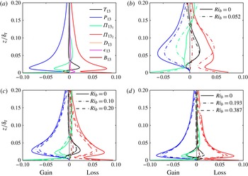
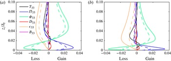
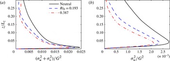
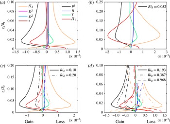
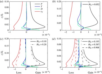
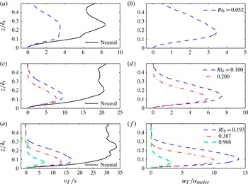
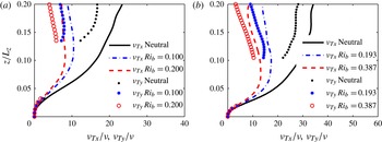
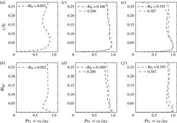
1. Introduction
Understanding and parametrizing turbulent fluxes in statically stable boundary layers, where buoyant forces destroy turbulence kinetic energy (TKE), remains a challenging yet very important problem in fluid dynamics (Ivey, Winters & Koseff Reference Ivey, Winters and Koseff2008; Fernando & Weil Reference Fernando and Weil2010). A stable flow of particular interest is the one in the atmospheric boundary layer (ABL), which roughly spans the lowest 0.2–2 km of the atmosphere and which is ubiquitously affected by stability (Stull Reference Stull1988). Arya (Reference Arya1968), Brost & Wyngaard (Reference Brost and Wyngaard1978), Nieuwstadt (Reference Nieuwstadt1984) and Hunt, Kaimal & Gaynor (Reference Hunt, Kaimal and Gaynor1985), among others, conducted experimental and numerical studies of the stable ABL to develop simple models for the mean profiles of turbulent quantities. Arya (Reference Arya1975) carried out experiments of flow on a flat plate with stabilizing temperature gradients and illustrated that the mean temperature and velocity profiles are affected by stability, in both the inner and outer layers. André et al. (Reference André, de Moor, Lacarrère and Du Vachat1978) developed a higher-order closure model for the diurnal evolution (where stability varies with time) of the ABL, which included equations for up to third-order statistics. Mahrt (Reference Mahrt1999) assessed the complications in modelling of stable layers and formulating surface flux parametrizations for numerical models. One such complication is that, under very stable conditions, turbulence in the atmosphere has been observed to collapse, at least intermittently. In a recent study, Flores & Riley (Reference Flores and Riley2011) developed a criterion for identifying such a collapse under strongly stable conditions using direct numerical simulations (DNS) of open channel flows. Van de Wiel et al. (Reference Van de Wiel, Moene, Jonker and Clercx2011) also discussed ABL conditions where winds become weak, resulting in very low levels of turbulence. They analysed these quasi-laminar flows using DNS and a simplified model to understand the collapse of turbulence.
While the earlier development of our understanding of flow and turbulence in the stable ABL was based on field experiments, particularly some of the crucial early experiments that date back to the 1960s and 1970s (Faller Reference Faller1963; Tatro & Mollo-Christensen Reference Tatro and Mollo-Christensen1967; Caldwell & Van Atta Reference Caldwell and Van Atta1970; Caldwell, Van Atta & Helland Reference Caldwell, Van Atta and Helland1972; Kaimal et al. Reference Kaimal, Wyngaard, Izumi and Coté1972), numerical simulations, with their ability to provide three-dimensional time-varying information on turbulent structures and dynamics, have recently emerged as a powerful tool to further our understanding of this problem. Some of the first numerical simulations of neutral and unstable (convective) boundary layers were carried out by Deardorff (Reference Deardorff1970, Reference Deardorff1972) using large eddy simulations (LES). Deardorff investigated profiles of turbulence statistics, the effect of buoyancy on mean profiles, and the effect of latitude upon turbulence and its structure. Later on, Mason & Thomson (Reference Mason and Thomson1987), Moeng & Sullivan (Reference Moeng and Sullivan1994), Cai & Steyn (Reference Cai and Steyn1996), Kosović & Curry (Reference Kosović and Curry2000), Bou-Zeid, Meneveau & Parlange (Reference Bou-Zeid, Meneveau and Parlange2004), Jiménez & Cuxart (Reference Jiménez and Cuxart2005), Bou-Zeid, Parlange & Meneveau (Reference Bou-Zeid, Parlange and Meneveau2007), Conzemius & Fedorovich (Reference Conzemius and Fedorovich2007), Stoll & Porté-Agel (Reference Stoll and Porté-Agel2008), Zhou & Chow (Reference Zhou and Chow2011) and Remmler & Hickel (Reference Remmler and Hickel2012), to name a few, also did similar studies of neutral and non-neutral ABL flows relying mainly on the LES technique with wall modelling (Pope Reference Pope2000). However, for flows under highly stable conditions, some uncertainties regarding the performance of LES remain, for two reasons. Firstly, owing to stability, there is a reduction in the size of the eddies (Mason & Derbyshire Reference Mason and Derbyshire1990; Andren Reference Andren1995). This reduces the fraction of the TKE that the simulation can resolve and the resolution with which the most energetic eddies are captured, and hence leads to an increased importance of the subgrid scales (SGS) and their models (Huang & Bou-Zeid Reference Huang and Bou-Zeid2013). Secondly, under strongly stable conditions, turbulence can become spatially and temporally intermittent as well as highly anisotropic (Ohya, Neff & Meroney Reference Ohya, Neff and Meroney1997; Mahrt Reference Mahrt1999); this invalidates some of the basic assumptions often used in developing SGS models, such as the statistical homogeneity of the horizontal dimensions and the applicability of Kolmogorov’s theories to the subgrid range of eddies.
While recent a priori (Bou-Zeid et al.
Reference Bou-Zeid, Higgins, Huwald, Meneveau and Parlange2010) and a posteriori (Kumar et al.
Reference Kumar, Kleissl, Meneveau and Parlange2006; Huang & Bou-Zeid Reference Huang and Bou-Zeid2013) studies tested and validated some facets of the LES approach for weak and moderate stabilities, their scope does not include very high stabilities, where the turbulence can become intermittent or completely damped. Furthermore, Taylor & Sarkar (Reference Taylor and Sarkar2008a
) recently investigated the Ekman layer under an external stratification using DNS, wall-resolved LES and wall-modelled LES; their main aim being to evaluate wall-resolved and wall-modelled LES, along with the investigation of the thermal properties of the Ekman layer. They observed that LES can capture mean velocity profiles well, but had biases in reproducing some higher-order quantities (fluxes near the top of the stable boundary layer). Higher-order statistics in LES are more sensitive to SGS contributions and models than the means, and increasingly higher resolutions are needed to accurately capture statistics of increasing orders. This was documented by Sullivan & Patton (Reference Sullivan and Patton2011) for the convective ABL and is expected to be even more critical in the stable ABL, where the contribution of the SGS increases with increasing stabilities. Hence, to probe in detail how stability modifies turbulent structure and higher-order budgets in this paper, we rely on DNS despite the limit that this technique imposes on the highest achievable Reynolds number. For example, Spalart, Coleman & Johnstone (Reference Spalart, Coleman and Johnstone2008, Reference Spalart, Coleman and Johnstone2009) could reach a maximum Reynolds number (based on the laminar Ekman boundary layer depth and the geostrophic wind speed) of 2000, while in the atmosphere the observed magnitude of this dimensionless number is
 ${\sim}10^{5}$
.
We thus perform a series of DNS at moderate Reynolds numbers with the aim of better understanding flow physics and improving current turbulence models under stable conditions. The set-up of the numerical experiments in this paper is very similar to the DNS studies on statically stable Ekman layers carried out by Coleman, Ferziger & Spalart (Reference Coleman, Ferziger and Spalart1992) at low Reynolds numbers. Coleman, Ferziger & Spalart (Reference Coleman, Ferziger and Spalart1990) and Coleman et al. (Reference Coleman, Ferziger and Spalart1992) examined the structural differences in neutral and stable Ekman layers by analysing quantities such as the vertical profiles of various parameters and the eddy size. They also evaluated some of the parametrizations recommended by Brost & Wyngaard (Reference Brost and Wyngaard1978), Nieuwstadt (Reference Nieuwstadt1984) and Hunt et al. (Reference Hunt, Kaimal and Gaynor1985) for stable ABLs. The main aim of Coleman et al. was to extrapolate, using theoretical arguments, certain DNS results to high Reynolds numbers applicable to ABLs. Their analysis suggests that the models proposed by Hunt et al. and Brost & Wyngaard are valid if the effects of varying Reynolds number are accounted for. They also show that simple gradient closures for temperature variance and heat flux are not very sensitive to Reynolds-number variation. Furthermore, Coleman (Reference Coleman1999) simulated neutral Ekman layers at a Reynolds number of 1000 based on the laminar Ekman boundary layer depth and geostrophic wind. He found that the flow has a distinct logarithmic region within a certain range of distances from the wall, and that the profiles of shear stress are indeed similar to the high-Reynolds-number flow simulated using LES by Andrén & Moeng (Reference Andrén and Moeng1993), but he did not find a complete Reynolds-number similarity. (Flow is said to show Reynolds-number similarity when ‘the motion of the energy-containing components of the turbulence are determined by the boundary conditions of the flow alone and are independent of the fluid viscosity, except so far as a change in the fluid viscosity may change the boundary conditions’ (see Townsend (Reference Townsend1956, p. 89) and Kunkel, Allen & Smits (Reference Kunkel, Allen and Smits2007)).) This suggests that further investigations of turbulent Ekman layers, where both the Reynolds (
 $\mathit{Re}$
) and Richardson (
 $\mathit{Ri}$
) numbers vary over wide ranges, are needed to further understand the effect of stability and to develop simple but accurate closures that are for example needed in weather and climate models. In this paper, we perform DNS with varying Reynolds and Richardson numbers to understand the physical mechanisms through which stability affects the budgets of first- and second-order quantities, with the long-term aim of developing improved physical models of turbulence in stable wall-bounded flows for any
 $(\mathit{Re},\mathit{Ri})$
combination.
One of the few studies with analysis of second-order budgets was performed by Garg et al. (Reference Garg, Ferziger, Monismith and Koseff2000), who investigated the budgets of TKE, fluxes and density variance in a channel flow using wall-resolved LES with a dynamic SGS model and showed that stability weakens the coupling between the inner and outer layers. Their Reynolds numbers based on the friction velocity
 $u_{\ast }$
were limited to 180 and 360, while in this paper, and owing to the increase in computational power since their paper came out, we are able to reach values exceeding 1180 (this corresponds to 900 based on laminar Ekman boundary layer depth and geostrophic wind speed). In addition, the Coriolis force was not included in their simulations and the flow in the upper part of the channel remained turbulent owing to mechanical production of turbulence at the upper wall, which would affect the bottom stable part of the flow in a channel but not in a boundary layer flow. Hattori, Houra & Nagano (Reference Hattori, Houra and Nagano2007), in their DNS of stable and unstable developing boundary layers also without the Coriolis force, examined the budgets of TKE, fluxes and temperature variance. The main aim of their study was to probe the near-wall structures and turbulent quantities under the influence of stability, and as such their simulations were performed at a constant Reynolds number, and only one stable simulation (with one Richardson number) was carried out. Marlatt, Waggy & Biringen (Reference Marlatt, Waggy and Biringen2010), on the other hand, analysed turbulence energy budgets in Ekman layer simulations, but did not study the effect of varying Richardson and Reynolds numbers. Hence, despite these important previous studies and others, the need for a comparative analysis of higher-order statistics in Ekman boundary layers at a range of Reynolds and Richardson numbers remains unfulfilled.
The primary goal of this study is thus to conduct such a comparative analysis. On an initially neutrally stratified and fully developed turbulent flow, a stable temperature profile is imposed with a constant temperature at the surface. Decreasing the surface temperature relative to the fluid temperature far from the wall increases the temperature gradient and the Richardson number, which is the dimensionless parameter we use here to quantify stability. The shape of the imposed profile is given in § 2. The main questions we aim to answer are these: (i) How does buoyancy in stable boundary layers affect higher-order turbulent quantities such as spectra and the various terms in the budget equations of TKE, fluxes and temperature variance? (ii) Are there mechanisms, other than direct buoyant destruction of TKE, through which stability acts on the flow and turbulence, and can the relative importance of the different mechanisms be quantified? (iii) Is Monin–Obukhov similarity theory (MOST) (Monin & Obukhov Reference Monin and Obukhov1954) valid under stable conditions and at the relatively low Reynolds numbers, compared to the ABL that we simulate.
In the next section, § 2, the equations and the set-up describing the flow simulated in this paper are presented. In § 3, we discuss the numerical methods used and the simulations carried out. Validation of the numerical methods and the code details are discussed in § 4. Section 5 presents the results and analyses, and § 6 contains the discussion and conclusions.
2. Governing equations and boundary conditions for DNS
The incompressible Navier–Stokes equations and the thermal energy budget equation, which govern the flow of a statically stable fluid, are numerically integrated in time. The momentum budget equations are solved in rotational form to ensure conservation of kinetic energy (Orszag & Pao Reference Orszag and Pao1974). The flow is driven by a steady pressure gradient, equivalent to a geostrophic forcing, and experiences steady homogeneous rotation resulting from the Coriolis force. We use the Boussinesq approximation to account for the effects of buoyancy in the flow. The governing equations are as follows:
 $$\begin{eqnarray}\displaystyle & \displaystyle \frac{\partial u_{i}}{\partial x_{i}}=0, & \displaystyle\end{eqnarray}$$
 $$\begin{eqnarray}\displaystyle & \displaystyle \frac{\partial u_{i}}{\partial t}+u_{j}\left(\frac{\partial u_{i}}{\partial x_{j}}-\frac{\partial u_{j}}{\partial x_{i}}\right)=-\frac{1}{{\it\rho}_{\infty }}\frac{\partial p^{\ast }}{\partial x_{i}}+2{\it\epsilon}_{ijk}{\it\Omega}_{j}(G_{k}-u_{k})+{\it\delta}_{i3}g{\it\Phi}+{\it\nu}\frac{\partial ^{2}u_{i}}{\partial x_{j}\partial x_{j}}, & \displaystyle\end{eqnarray}$$
 $$\begin{eqnarray}\displaystyle & \displaystyle \frac{\partial {\it\Phi}}{\partial t}+u_{i}\frac{\partial {\it\Phi}}{\partial x_{i}}={\it\alpha}\frac{\partial ^{2}{\it\Phi}}{\partial x_{j}\partial x_{j}}, & \displaystyle\end{eqnarray}$$
 $$\begin{eqnarray}\displaystyle & \displaystyle p^{\ast }=p+{\textstyle \frac{1}{2}}{\it\rho}_{\infty }u_{j}u_{j}, & \displaystyle\end{eqnarray}$$
 $$\begin{eqnarray}\displaystyle & \displaystyle \frac{\partial P}{\partial x_{i}}=-2{\it\rho}_{\infty }{\it\epsilon}_{ijk}{\it\Omega}_{j}G_{k}+{\it\delta}_{i3}{\it\rho}_{\infty }g, & \displaystyle\end{eqnarray}$$
 $$\begin{eqnarray}\displaystyle & \displaystyle {\it\Phi}=({\it\theta}-{\it\theta}_{\infty })/{\it\theta}_{\infty }. & \displaystyle\end{eqnarray}$$
 $u_{i}$
is the velocity vector;
 ${\it\theta}$
is the local potential temperature and
 ${\it\theta}_{\infty }$
is the constant reference potential temperature;
 $g=9.81\ \text{m}^{2}\ \text{s}^{-1}$
is the gravitational acceleration;
 ${\it\epsilon}_{ijk}$
is the alternating unit tensor, with
 $i,j,k$
running from 1 to 3;
 ${\it\delta}_{i3}$
is the Kronecker delta;
 ${\it\Omega}_{j}$
is the angular velocity vector of the Earth and is in the opposite direction to gravity (the summations use the ‘
 $f$
-plane’ approximation; see Zikanov, Slinn & Dhanak (Reference Zikanov, Slinn and Dhanak2003) for details on the effect of a non-zero horizontal component of the Earth’s rotation vector);
 $G_{k}$
is the geostrophic wind vector;
 $p$
is the pressure deviation from the mean pressure (
 $P$
) field imposed via the geostrophic forcing and the mean hydrostatic balance;
 ${\it\rho}_{\infty }$
is a constant reference density;
 $p^{\ast }$
is the modified perturbation pressure that is computed by solving a Poisson equation (resulting from taking the divergence of the momentum equation and using the continuity equation) at each time step; and
 ${\it\nu}$
and
 ${\it\alpha}$
are the kinematic viscosity and thermal diffusivity, respectively (both assumed to be constant). Note that the actual potential temperature conservation equation has the term
 ${\it\alpha}({\it\theta}/T)\,\partial ^{2}T/\partial x_{j}\partial x_{j}$
, where
 $T$
is the temperature. But at the small scales where thermal diffusivity is important, the ratio
 ${\it\theta}/T$
varies negligibly in space (and can be brought inside the Laplacian operator) and hence the diffusion term simplifies to
 ${\it\alpha}\,\partial ^{2}{\it\theta}/\partial x_{j}\partial x_{j}$
(Wyngaard Reference Wyngaard2010). In the set of equations that we solve, this term results in
 ${\it\alpha}\,\partial ^{2}{\it\Phi}/\partial x_{j}\partial x_{j}$
.
Horizontal boundary conditions are periodic. Vertical boundary conditions consist of no-slip (
 $u=0$
and
 $v=0$
) and impermeability (
 $w=0$
), with a smooth wall at the bottom surface, and a stress-free impermeable boundary, with zero heat flux, at the top of the domain:
 $$\begin{eqnarray}\frac{\partial u}{\partial z}=\frac{\partial v}{\partial z}=w=0\quad \text{and}\quad \frac{\partial {\it\theta}}{\partial z}=0\quad \text{at the top}.\end{eqnarray}$$
A constant temperature, which is lower than the temperature
 ${\it\theta}_{\infty }$
above the boundary layer, is imposed at the wall; this results in a downward stabilizing heat flux across the whole boundary layer that varies with time. Consequently, a stationary state is not attained in simulations with stable stratification. However, the change in downward heat flux is sufficiently slow such that a quasi-steady state is reached where the turbulence is very close to equilibrium with the mean fields at any time. This set-up is very similar to the one used by Coleman et al. (Reference Coleman, Ferziger and Spalart1992) and is representative of stable flows in the atmospheric Ekman boundary layers. For stable flows in the oceanic Ekman boundary layers, an open channel flow with heat flux applied at the free surface (with the atmosphere) and no heat flux (adiabatic conditions) at the bottom wall (ocean floor) is usually simulated as in the LES of Taylor & Sarkar (Reference Taylor and Sarkar2008b
).
The initial temperature profile (Coleman et al. Reference Coleman, Ferziger and Spalart1992) is given by the following equation:
 $$\begin{eqnarray}{\it\theta}(z)=\frac{a_{\ast }}{2}\left(\frac{-{\rm\pi}}{\ln (0.01)}\right)^{1/2}{\it\Gamma}_{0,0}\;\text{erf}\left(\frac{z/a_{\ast }}{(-\ln (0.01))^{-1/2}}\right)+{\it\theta}_{0}.\end{eqnarray}$$
Here erf is the error function;
 ${\it\Gamma}_{0,0}$
is the initial vertical temperature gradient at the surface (the vertical temperature gradient is
 ${\it\Gamma}=\text{d}\langle {\it\theta}\rangle /\text{d}z$
, with angle brackets
 $\langle \;\rangle$
indicating Reynolds averaging throughout the paper);
 ${\it\theta}_{0}$
is the surface temperature, which remains fixed throughout any given simulation; and
 $a_{\ast }$
is the height where the vertical temperature gradient
 $\text{d}\langle {\it\theta}\rangle /\text{d}z$
is approximately 1 % of
 ${\it\Gamma}_{0,0}$
. Throughout this paper, a single 0 subscript is used to indicate surface values and a double (
 $0,0$
) subscript is used to indicate surface values at initial time,
 $t=0$
. Further details about the initialization of the temperature field can be found in Coleman et al. (Reference Coleman, Ferziger and Spalart1992). Note, however, that since we impose a constant temperature at the surface and run the simulations for sufficiently long periods before starting to compute statistics (further details in the next section), the effect of the initialization on the results should be negligible.
Some of the important non-dimensionalization variables we will use include: the Coriolis parameter
 $f=2\Vert {\it\bf\Omega}\Vert \sin {\it\phi}$
, where
 $\Vert {\it\bf\Omega}\Vert$
is the magnitude of the angular velocity (that is, the rotation rate) of the Earth and
 ${\it\phi}$
is the latitude (here we assume a latitude of 90°, giving a value of
 $f=1.454\times 10^{-4}\ \text{rad}\ \text{s}^{-1}$
and the largest Coriolis effect); the laminar Ekman layer depth
 $D=(2{\it\nu}/f)^{1/2}\approx 0.4$
m; and the neutral-case turbulent Ekman layer length scale
 ${\it\delta}_{t}=u_{\ast }/f$
. A good approximation of the actual neutral Ekman boundary layer depth in our simulations would be
 $C_{h}u_{\ast }/f$
, where
 $C_{h}=0.7$
is a constant. The range of values of
 $C_{h}$
used in the literature vary from 0.5 to 0.7 (Caldwell et al.
Reference Caldwell, Van Atta and Helland1972; Coleman et al.
Reference Coleman, Ferziger and Spalart1990; Zilitinkevich & Mironov Reference Zilitinkevich and Mironov1996). The friction velocity
 $u_{\ast }$
is defined as
 $$\begin{eqnarray}u_{\ast }=\left[\left({\it\nu}\frac{\partial u}{\partial z}\right)^{2}|_{0}+\left({\it\nu}\frac{\partial v}{\partial z}\right)^{2}|_{0}\right]^{1/2},\end{eqnarray}$$
where the subscript 0 indicates that the gradients are taken at the surface.
The important set of non-dimensional parameters based on these variables includes: the Reynolds number
 $\mathit{Re}_{f}=GD/{\it\nu}=G/({\it\nu}f/2)^{1/2}$
; the bulk Reynolds number
 $\mathit{Re}_{{\it\delta}_{t}}=G{\it\delta}_{t}/{\it\nu}$
; the surface (initial) Richardson number
 $\mathit{Ri}_{0,0}=g{\it\Gamma}_{0,0}D^{2}/{\it\theta}_{\infty }G^{2}$
; the bulk Richardson number
 $\mathit{Ri}_{b}=g{\rm\Delta}{\it\theta}{\it\delta}_{t}/{\it\theta}_{\infty }G^{2}$
, where
 ${\rm\Delta}{\it\theta}={\it\theta}_{\infty }-{\it\theta}_{s}$
; the Prandtl number
 $\mathit{Pr}={\it\nu}/{\it\alpha}=0.7$
; the non-dimensional thermal length scales
 $L_{V}=a_{\ast }/D$
and
 $L_{T}=a_{\ast }/{\it\delta}_{t}$
; and the non-dimensional time
 $t_{s}=tf$
. Note that
 $U_{g}$
is the
 $x$
component of
 $\boldsymbol{G}$
, but since the imposed mean geostrophic wind is aligned with the
 $x$
direction,
 $U_{g}$
and
 $G$
(the magnitude of
 $\boldsymbol{G}$
) are the same.
3. Physical and numerical set-up of the simulations
The code used here was initially developed as an LES code by Albertson & Parlange (Reference Albertson and Parlange1999a
,Reference Albertson and Parlange
b
) and later modified by Porté-Agel, Meneveau & Parlange (Reference Porté-Agel, Meneveau and Parlange2000) and Bou-Zeid, Meneveau & Parlange (Reference Bou-Zeid, Meneveau and Parlange2005). For the current DNS, it was further modified by Shah & Bou-Zeid (Reference Shah and Bou-Zeid2012). The domain is periodic in the spanwise
 $y$
and streamwise
 $x$
directions, which are also associated with the use of pseudo-spectral numerical schemes. A second-order centred-difference scheme on a uniform staggered grid is used in the vertical (
 $z$
) direction. Time integration is carried out using the second-order Adams–Bashforth scheme. Nonlinear terms are dealiased using the
 $\frac{3}{2}$
rule (Orszag Reference Orszag1971). Message passing interface (MPI) is used to carry out the simulations on multiple cores. Simulations at Reynolds numbers (
 $\mathit{Re}_{f}$
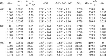
) of 400, 600 and 900 were carried out on 128, 288 and 416 cores, respectively, on computing clusters at the National Center for Atmospheric Research and at Princeton University. In total, 15 cases were simulated.
Simulation parameters.
 $\text{}^{\dagger }$
For the highest stability cases where intermittency occurs, the values of the friction velocity
 $u_{\ast }$
(and hence the corresponding
 ${\it\delta}_{t}$
, wall units and
 $\mathit{Re}_{{\it\tau}}$
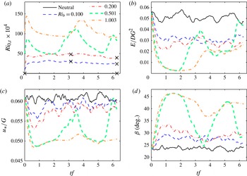
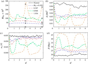
) are not very meaningful owing to the large-amplitude oscillatory behaviour with periods comparable to the simulation time (larger than averaging time); see figures 7(c), 8(c) and 9(c).

3.1. Physical parameters
The details of all simulations are listed in table 1. Unlike Coleman et al. (Reference Coleman, Ferziger and Spalart1990, Reference Coleman, Ferziger and Spalart1992), here we vary both parameters: the Reynolds number (
 $\mathit{Re}_{f}$
) from 400 to 900, and the surface Richardson number (
 $\mathit{Ri}_{0,0}$
) from 0 to 0.010. Parameters that have been kept constant are the latitude
 ${\it\phi}=90^{\circ }$
, which was selected to give the largest Coriolis effect, the Prandtl number (
 $\mathit{Pr}=0.7$
for air) and the ratio of the initial thermal length scale to the approximate turbulent length scale
 $L_{T}=a_{\ast }/{\it\delta}_{t}=0.75$
. The value used here for
 $a_{\ast }$
corresponds to a late-night or early-morning temperature profile over land, where the effect of lower surface temperature has reached larger heights. Some analysis with temperature profiles corresponding to early evening can be found in Coleman et al. (Reference Coleman, Ferziger and Spalart1992). For the three Reynolds numbers (
 $\mathit{Re}_{f}=400,600,900$
), the geostrophic wind speeds
 $G$
are 0.0115, 0.0172 and
 $0.0259\ \text{m}\ \text{s}^{-1}$
, respectively; the domain sizes are
 $L_{x}\times L_{y}\times L_{z}=26D\times 26D\times 24D$
,
 $36D\times 36D\times 25D$
and
 $50D\times 50D\times 33D$
, respectively; and the heights of the computational domains in terms of the dynamically simulated boundary layer depths are approximately
 $2{\it\delta}_{t}$
,
 $1.5{\it\delta}_{t}$
and
 $1.33{\it\delta}_{t}$
, respectively.
Coleman et al. (Reference Coleman, Ferziger and Spalart1992) found that
 $\mathit{Ri}_{0,0}\sim 0.001$
is about the maximum surface Richardson number that can be imposed on a neutral flow with
 $\mathit{Re}_{f}=400$
before laminarization occurs. Our simulation results agree with findings of Coleman et al. (Reference Coleman, Ferziger and Spalart1992); for higher surface Richardson number (0.005 and 0.010) at
 $\mathit{Re}_{f}=400$
, the flow in our simulations laminarizes or becomes intermittently turbulent. However, we observed that, for
 $\mathit{Ri}_{0,0}=0.002$
, turbulence intensity dies down to very small values, and then increases again after build-up of shear, resulting in an intermittently turbulent boundary layer. With a higher Reynolds number (
 $\mathit{Re}_{f}=600$
), the surface Richardson number
 $\mathit{Ri}_{0,0}$
where this intermittent behaviour in TKE is seen increases to around 0.005, while for
 $\mathit{Ri}_{0,0}=0.010$
the flow laminarizes almost completely. At
 $\mathit{Re}_{f}=900$
, the flow remains fully and steadily turbulent up to
 $\mathit{Ri}_{0,0}=0.005$
; therefore, the hypothesized increase in the critical Richardson number with increasing Reynolds number (Schlichting Reference Schlichting1979; Katul et al.
Reference Katul, Porporato, Shah and Bou-Zeid2014) is further supported by these findings.
The horizontal extent of the domain is governed by the ability to capture the largest dynamically important turbulent scales. Jiménez (Reference Jiménez1998), Abe & Kawamura (Reference Abe, Kawamura and Castro2002) and others have indicated the existence of very large-scale structures in wall flows that could require very large simulation domains. However, Coleman et al. (Reference Coleman, Ferziger and Spalart1990) found no evidence of such large-scale structures in their studies. Shingai & Kawamura (Reference Shingai and Kawamura2004) studied neutral Ekman layers at higher Reynolds numbers and on larger domains than Coleman et al. (Reference Coleman, Ferziger and Spalart1990) to verify the existence of these large-scale structures. They observe that energy spectra and two-point correlations do indicate the existence of large-scale structures away from the wall; however, turbulence statistics near the surface were not affected by the size of the computational domain and averaging time, which suggests that these very large-scale structures are not very active dynamically near the wall. To ensure that our results and conclusions are not dependent on the domain size, we performed a simulation for one of the cases (
 $\mathit{Re}_{f}=600$
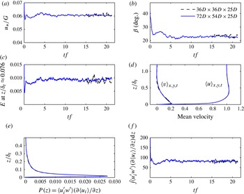
with neutral stratification) using a larger domain (twice the length and 1.5 times the width) and found no discernible impact on the computed statistics that we analyse in this study (see appendix A). However, we cannot rule out that other statistics we do not compute here or statistics in simulations that exhibit intermittency might be sensitive to the size of the periodic domain (García-Villalba & Del Álamo Reference García-Villalba and Del Álamo2011). For this and other reasons detailed later, we will refrain from analysing averaged statistics of intermittent simulations and will focus on those not exhibiting intermittency.
3.2. Numerical parameters
Computations for all cases at a particular Reynolds number were performed using the same number of grid points for all stabilities; the corresponding grid resolution, domain sizes and other simulation parameters are given in table 1. As Coleman et al. (Reference Coleman, Ferziger and Spalart1992) argue, vorticity fluctuations are reduced in the stable cases and so is the rate of dissipation of kinetic energy throughout the domain. Even if stability dampens some of the largest length scales present, the Kolmogorov scale (
 ${\it\eta}$
) will be larger in the stable cases than in the neutral one with the same
 $\mathit{Re}_{f}$
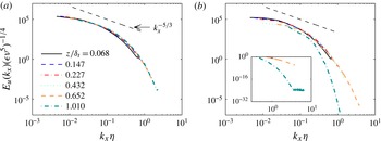
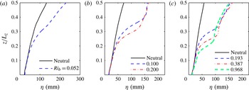
(see appendix B for detailed profiles of the Kolmogorov length scale). This can also be verified from figure 1. Here we plot the normalized streamwise velocity spectra against the normalized wavenumber at different heights
 $z/{\it\delta}_{t}$
, for
 $\mathit{Re}_{f}=900$
. The energy content at all the levels decreases with stability. For the stable case, the spectra drop faster with increasing wavenumber in the viscous range compared to the neutral case, particularly for the higher elevations. For the highest level analysed, which is near the top of the boundary layer, the inset in figure 1(b) clearly shows that the smallest scales in the stable case are over-resolved. Similarly, the smallest scale over which fluctuations in the scalar field are maintained is given by the Batchelor scale
 ${\it\eta}_{s}$
, which for a Prandtl number
 ${<}1$
is larger than
 ${\it\eta}$
(Tennekes & Lumley Reference Tennekes and Lumley1972). Hence, the number of points used for a neutral case is necessarily also sufficient to capture the Kolmogorov and Batchelor scale eddies in the stable cases at the same Reynolds number. A further requirement in DNS is the proper resolution of the viscous sublayer, which extends up to
 $z^{+}=10$
. We ensure this by placing around 10 points in that sublayer in the neutral simulations, to yield a non-dimensional grid spacing in wall units
 ${\rm\Delta}z^{+}={\rm\Delta}zu_{\ast }/{\it\nu}\approx 1$
, where
 ${\rm\Delta}z$
is the constant grid spacing in the vertical direction. Again, this is more than sufficient for the stable cases at the same
 $\mathit{Re}$
in which we maintain the same dimensional
 ${\rm\Delta}z$
: the friction velocity at the surface is reduced for stronger stability simulations, leading to a reduction in the grid spacing in wall units
 ${\rm\Delta}z^{+}$
, as reported in table 1, and hence to a better resolution of the viscous sublayer.
Streamwise velocity spectra for (a) neutral case (
 $\mathit{Ri}_{0,0}=0$
) and (b) stable case with
 $\mathit{Ri}_{0,0}=0.002$
at
 $\mathit{Re}_{f}=900$
. The spectral energy is non-dimensionalized using the plane-averaged dissipation at that height (
 ${\it\epsilon}=2{\it\nu}\langle (\partial u_{i}^{\prime }/\partial x_{j})(\partial u_{i}^{\prime }/\partial x_{j})\rangle$
) and the molecular viscosity (
 ${\it\nu}$
), while the wavenumber is non-dimensionalized by the Kolmogorov scale (
 ${\it\eta}=({\it\nu}^{3}/{\it\epsilon})^{1/4}$
) at that height. The
 $-\frac{5}{3}$
slope corresponding to the inertial subrange is also depicted. The inset in panel (b) shows a plot of the spectra at the higher levels and wavenumbers. Here the height is normalized by the neutral-case turbulent length scale
 ${\it\delta}_{t}$
so that we can compare spectra at the same physical height in the stable and neutral cases.

Simulations are run for at least 60 physical hours with no static stability (i.e. neutral case) as a warm-up to allow the flow field to fully develop before any statistics are collected for analysis. Initial conditions imposed for these warm-up runs were laminar profiles with random perturbations of approximately 5 % of the free-stream values. The flow fields at the end of these warm-up runs (for different Reynolds numbers) are subsequently used to initialize the runs used to generate the analyses data; the analyses simulations are run for one inertial period
 $=2{\rm\pi}/f$
(here
 $f=2{\it\omega}\sin ({\rm\pi}/2)=2{\it\omega}=2\times 2{\rm\pi}\ \text{rad}/24\ \text{h}$
; thus one inertial period
 $=12\ \text{h}$
), for both neutral and stable cases. However, for cases with stability, the initial temperature profile and the constant lower surface temperature are imposed on these velocity fields and the buoyancy term is added to the momentum equations. While stable cases are run for one inertial period, the data used for analysis of these cases are from the last half of this period. This is intended to allow the stable simulations to reach a quasi-equilibrium state and overcome the influence of the initial temperature profile. Perturbations do not need to be added to the initial temperature field (Coleman et al.
Reference Coleman, Ferziger and Spalart1992) for the stable cases; they emerge dynamically as a result of perturbations in the velocity field.
The time step (
 ${\rm\Delta}t^{+}={\rm\Delta}tu_{\ast }^{2}/{\it\nu}$
) for the neutral cases is around 0.015 (
 ${\rm\Delta}t^{+}=0.011$
, 0.0104 and 0.017 for
 $\mathit{Re}_{f}=400$
, 600 and 900, respectively). The corresponding dimensional time steps thus ranged from 0.1 to 0.225 s. For stable cases, since the friction velocity is smaller than the neutral value, the time steps in inner coordinates are also somewhat smaller.
3.3. Statistics
Throughout this paper, the notation used is as follows:
 $u_{j}=\langle u_{j}\rangle +u_{j}^{\prime }=U_{j}+u_{j}^{\prime }$
,
 $p=\langle p\rangle +p^{\prime }$
,
 ${\it\rho}=\langle {\it\rho}\rangle +{\it\rho}^{\prime }$
and
 ${\it\theta}=\langle {\it\theta}\rangle +{\it\theta}^{\prime }$
, where angle brackets
 $\langle \;\rangle$
indicate Reynolds averaging and primes (
 $^{\prime }$
) indicate the fluctuating component. Subscripts denoting directions
 $x$
,
 $y$
and
 $z$
are used interchangeably with 1, 2 and 3, respectively. Pressure is computed from the modified pressure solved for by the DNS code by subtracting the trace term as per (2.4). Averaging has been carried out over
 $xy$
planes and in time
 $t$
, at each
 $z$
, for about half an inertial period, or
 ${\rm\pi}/f$
seconds, unless otherwise noted. The start and end points of the averaging period are later indicated in the surface Richardson number plots (for example 7
a) by cross marks.
4. Validation
4.1. Neutral mean profiles
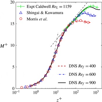
We first present basic plots to validate our methodology and the DNS code. Figure 2 shows the mean velocity profiles for the neutrally stratified cases at various Reynolds numbers in comparison with the experimental studies of Caldwell & Van Atta (Reference Caldwell and Van Atta1970) and the numerical simulations of Shingai & Kawamura (Reference Shingai and Kawamura2004) and Morris, Handler & Rouson (Reference Morris, Handler and Rouson2011). Our simulations reproduce the log law (given by
 $M^{+}=(1/{\it\kappa})\log (z^{+})+B$
, where
 $M=\sqrt{\langle u\rangle ^{2}+\langle v\rangle ^{2}}$
is the mean streamwise velocity magnitude,
 ${\it\kappa}$
is the von Kármán constant and
 $B=5.5$
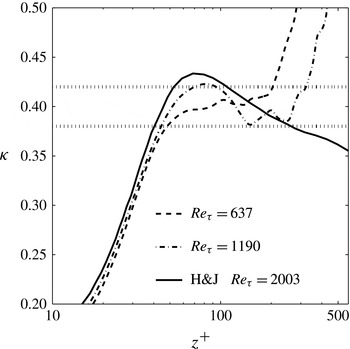
is a constant) very well in the higher-Reynolds-number simulations where a log region exists, and match both the experiments and the other simulations. The simulated log region can also be observed in figure 3, where a plateau of relatively constant
 ${\it\kappa}$
, depicting the slope in the log region, is seen (Marlatt, Waggy & Biringen Reference Marlatt, Waggy and Biringen2011), particularly for the simulation with
 $\mathit{Re}_{f}=900$
. The value of the von Kármán constant
 ${\it\kappa}$
for this Ekman layer with turning is computed using the following surface layer similarity relationship (Stull Reference Stull1988):
 $$\begin{eqnarray}\frac{{\it\kappa}z}{u_{\ast }}\left[\left(\frac{\partial \langle u\rangle }{\partial z}\right)^{2}+\left(\frac{\partial \langle v\rangle }{\partial z}\right)^{2}\right]^{1/2}=1.\end{eqnarray}$$
The exact value of
 ${\it\kappa}$
is not precisely known, and whether its value is truly constant over the log region remains the subject of debate. However, experiments in laboratories, in the atmosphere and DNS indicate relatively constant (compared to its variation with height outside of the log region) values ranging from 0.38 to 0.42 (Miyashita, Iwamoto & Kawamura Reference Miyashita, Iwamoto and Kawamura2006; Spalart et al.
Reference Spalart, Coleman and Johnstone2008, Reference Spalart, Coleman and Johnstone2009; Marlatt et al.
Reference Marlatt, Waggy and Biringen2011). The above equation can be further written in inner coordinates as
 $$\begin{eqnarray}\frac{1}{{\it\kappa}}=z^{+}\left[\left(\frac{\partial \langle u^{+}\rangle }{\partial z^{+}}\right)^{2}+\left(\frac{\partial \langle v^{+}\rangle }{\partial z^{+}}\right)^{2}\right]^{1/2},\end{eqnarray}$$
where
 $u^{+}=u/u_{\ast }$
and
 $z^{+}=z\ u_{\ast }/{\it\nu}$
. The values we obtain for the simulations with
 $\mathit{Re}_{f}=600$
and
 $\mathit{Re}_{f}=900$
fall within the range reported by other studies over more than 100 wall units (the log layer in the
 $\mathit{Re}_{f}=400$
simulation is too thin to compute a value).
Mean velocity profiles for neutral cases at different Reynolds numbers, in comparison with numerical studies (Shingai & Kawamura Reference Shingai and Kawamura2004; Morris et al.
Reference Morris, Handler and Rouson2011) and experimental observations (Caldwell et al. (Reference Caldwell, Van Atta and Helland1972); at a comparable Reynolds number of
 $\mathit{Re}_{L}=G/\sqrt{{\it\nu}{\it\omega}_{p}}=1159$
, where
 ${\it\omega}_{p}$
is the speed of rotation in Caldwell’s experiments).

The von Kármán measure for the neutral case with
 $\mathit{Re}_{{\it\tau}}=637$
(
 $\mathit{Re}_{f}=600$
) and 1190 (
 $\mathit{Re}_{f}=900$
) in comparison with channel flow at
 $\mathit{Re}_{{\it\tau}}=2003$
(Hoyas & Jiménez Reference Hoyas and Jiménez2006; Spalart et al.
Reference Spalart, Coleman and Johnstone2009). Typical range of values of von Kármán constant
 ${\it\kappa}$
reported in the literature (0.38–0.42) is indicated by the two black dotted lines.

4.2. Velocity and temperature spectra
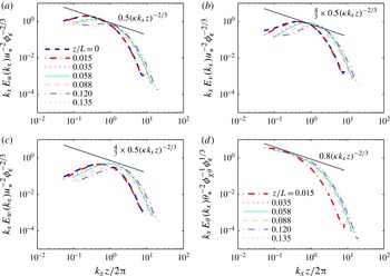
In figure 4, we plot one-dimensional (streamwise) normalized premultiplied spectra of each of the three velocity components and temperature against normalized wavenumber at different levels of stability (at
 $\mathit{Re}_{f}=900$
and
 $\mathit{Ri}_{0,0}=0.001,0.002,0.005$
) defined by the parameter
 $z/L$
, where
 $$\begin{eqnarray}L=-\frac{u_{\ast }^{3}{\it\theta}_{\infty }}{{\it\kappa}gH_{k,s}}\end{eqnarray}$$
is the Obukhov length. Here,
 ${\it\theta}_{\infty }$
is the reference temperature; and
 $H_{k,s}=-{\it\alpha}\,\text{d}\langle {\it\theta}\rangle /\text{d}z|_{0}$
is the surface kinematic heat flux, with
 ${\it\alpha}=k/{\it\rho}C_{p}$
the thermal diffusivity of air, where
 $k$
is the thermal conductivity,
 ${\it\rho}$
the density and
 $C_{p}$
the specific heat capacity of air. The spectra are normalized using the Monin–Obukhov similarity parameters
 $u_{\ast }$
,
 ${\it\theta}_{\ast }$
and
 $z$
, where
 ${\it\theta}_{\ast }=-H_{k,s}/u_{\ast }$
is a surface temperature scale (Kaimal et al.
Reference Kaimal, Wyngaard, Izumi and Coté1972; Wyngaard & Coté Reference Wyngaard and Coté1972; Chung & Matheou Reference Chung and Matheou2012). In the inertial range, dimensional arguments (see e.g. Kaimal et al.
Reference Kaimal, Wyngaard, Izumi and Coté1972) lead to the following expressions for these spectra (we write only the equations for the
 $u$
and
 ${\it\theta}$
spectra; the equations for the spectra of
 $v$
and
 $w$
are similar to
 $u$
but with an additional
 $\frac{4}{3}$
factor on the right-hand side):
 $$\begin{eqnarray}\displaystyle \displaystyle \frac{k_{x}E_{u}(k_{x})}{u_{\ast }^{2}} & = & \displaystyle \displaystyle \frac{{\it\beta}_{1}}{{\it\kappa}^{2/3}}{\it\phi}_{{\it\epsilon}}^{2/3}(k_{x}z)^{-2/3},\end{eqnarray}$$
 $$\begin{eqnarray}\displaystyle \displaystyle \frac{k_{x}E_{{\it\theta}}(k_{x})}{{\it\theta}_{\ast }^{2}} & = & \displaystyle \displaystyle \frac{{\it\beta}_{2}}{{\it\kappa}^{2/3}}{\it\phi}_{{\it\epsilon}}^{-1/3}{\it\phi}_{{\it\chi}_{{\it\theta}}}(k_{x}z)^{-2/3}.\end{eqnarray}$$
 ${\it\beta}_{1}\approx 0.5$
and
 ${\it\beta}_{2}\approx 0.8$
(Kaimal et al.
Reference Kaimal, Wyngaard, Izumi and Coté1972);
 ${\it\phi}_{{\it\epsilon}}={\it\epsilon}{\it\kappa}z/u_{\ast }^{3}$
and
 ${\it\phi}_{{\it\chi}_{{\it\theta}}}={\it\chi}_{{\it\theta}}{\it\kappa}z/(u_{\ast }{\it\theta}_{\ast }^{2})$
are the non-dimensional dissipation rates for TKE and
 $\langle {\it\theta}^{\prime }{\it\theta}^{\prime }\rangle /2$
, respectively (
 ${\it\chi}_{{\it\theta}}={\it\epsilon}_{{\it\theta}}/2$
, where
 ${\it\epsilon}_{{\it\theta}}$
is the molecular dissipation of temperature variance);
 $k_{x}$
is the wavenumber and
 ${\it\kappa}=0.41$
is used. The advantage of this non-dimensionalization is that, regardless of the level of static stability imposed on the flow, the spectra collapse in the inertial subrange (if the Reynolds number is high enough for the subrange to exist) on to a
 $-\frac{2}{3}$
power law. One can then examine the energy content of the larger scales as a function of
 $z/L$
.
Streamwise velocity and temperature spectra: (a)
 $u$
, (b)
 $v$
, (c)
 $w$
and (d)
 ${\it\theta}$
at
 $\mathit{Re}_{f}=900$
with varying static stabilities defined by the parameter
 $z/L$
. Various
 $z/L$
values are obtained by considering simulations with different
 $\mathit{Ri}_{0,0}$
at the same
 $\mathit{Re}_{f}=900$
. The heights of the spectra are selected to fall approximately in the inertial layer; they correspond to
 $z/{\it\delta}_{t,neutral}$
of 0.0325, 0.0587, 0.0785 and 0.0896, which in wall units are approximately at
 $z^{+}$
of 40, 72, 96 and 110. The spectral energy is normalized using the plane-averaged dissipation rates (
 ${\it\epsilon}$
and
 ${\it\chi}_{{\it\theta}}$
) at that height. The
 $-\frac{2}{3}$
slope corresponding to the inertial subrange is depicted with a straight solid black line in all the panels.

In neutral and near-neutral cases (
 $z/L\approx 0$
), there is a small inertial subrange indicated by the segments of the spectra with a slope of
 $-\frac{2}{3}$
(given the Reynolds number, the extent of the inertial subrange is limited as one would expect). Higher-Reynolds-number simulations will be useful to further confirm the continuous presence of an inertial subrange as stability increases. At the lower end of the wavenumbers, the spectral lines for different values of
 $z/L$
bifurcate, as has been observed by Kaimal et al. (Reference Kaimal, Wyngaard, Izumi and Coté1972). The overall behaviour at all scales agrees quite well with the generally observed spectra in ABLs (also observable in figure 1): the energy peak shifts to higher wavenumbers and the energy content of the large scales at different heights drops with increasing stability, indicating that the buoyancy damping is mostly affecting the larger scales (in agreement with LES results reported in Huang & Bou-Zeid (Reference Huang and Bou-Zeid2013)). This reduces the span of scales that fall in the inertial subrange. The amount of energy decreases with increasing stability parameter
 $z/L$
, again underlining the important effect of buoyancy on the total TKE content away from the wall (as
 $z$
increases or
 $L$
decreases,
 $z/L$
increases).
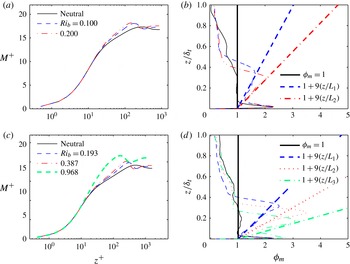
(a,c) Mean velocity profiles in inner coordinates,
 $M^{+}=M/u_{\ast }$
, for (a)
 $\mathit{Re}_{f}=600$
and (c)
 $\mathit{Re}_{f}=900$
and (b,d) the respective mean non-dimensional velocity gradients
 ${\it\phi}_{m}$
. In panels (b,d), the solid black thick line gives the neutral-case constant non-dimensional velocity gradient, while the other thick lines are gradients predicted by MOST (Monin & Obukhov Reference Monin and Obukhov1954),
 ${\it\phi}_{m}=1+{\it\beta}_{m}(z/L)$
, for various stabilities; the thin lines are the corresponding simulated profiles. In panel (b), the dashed line (blue online) corresponds to
 $\mathit{Ri}_{b}=0.100$
and the dot-dashed line (red online) corresponds to
 $\mathit{Ri}_{b}=0.200$
, both at
 $\mathit{Re}_{f}=600$
; here
 $L_{1}$
and
 $L_{2}$
denote the Obukhov lengths at
 $\mathit{Ri}_{b}=0.100$
and
 $\mathit{Ri}_{b}=0.200$
, respectively. In panel (d), the dashed line (blue online) corresponds to
 $\mathit{Ri}_{b}=0.193$
, the dotted line (red online) corresponds to
 $\mathit{Ri}_{b}=0.387$
and the dot-dashed line (green online) corresponds to
 $\mathit{Ri}_{b}=0.968$
, all at
 $\mathit{Re}_{f}=900$
; here,
 $L_{1}$
,
 $L_{2}$
and
 $L_{3}$
denote the Obukhov lengths at
 $\mathit{Ri}_{b}=0.193$
, 0.387 and 0.968, respectively. Note that the non-dimensionalization length scale in the vertical (
 $y$
axis) in panels (b) and (d) is the depth
 ${\it\delta}_{t}$
of the neutral case at that
 $\mathit{Re}_{f}$
.

5. Results
5.1. Mean profiles with stability
Log-linear plots similar to the one in figure 2, but with positive Richardson numbers, are compared to the neutral case in figure 5(a,c), which correspond to
 $\mathit{Re}_{f}$
of 600 and 900, respectively. A correction to the log law in stably stratified cases was given by Monin & Obukhov (Reference Monin and Obukhov1954). The MOST, which theoretically holds for infinite Reynolds number only, postulates that the non-dimensional velocity and temperature gradients (
 ${\it\phi}_{m}$
and
 ${\it\phi}_{h}$
, respectively) for non-neutral cases are functions of the height normalized by the Obukhov length
 $L$
. These functions have been experimentally shown to be linear in
 $z/L$
(for
 $0\leqslant z/L<1$
) in stable conditions (Brutsaert Reference Brutsaert1982; Stull Reference Stull1988; see also theoretical justification in Li, Katul & Bou-Zeid (Reference Li, Katul and Bou-Zeid2012)):
 $$\begin{eqnarray}\displaystyle & \displaystyle {\it\phi}_{m}\biggl(\frac{z}{L}\biggr)=\frac{{\it\kappa}z}{u_{\ast }}\left[\left(\frac{\partial \langle u\rangle }{\partial z}\right)^{2}+\left(\frac{\partial \langle v\rangle }{\partial z}\right)^{2}\right]^{1/2}=1+{\it\beta}_{m}\frac{z}{L}, & \displaystyle\end{eqnarray}$$
 $$\begin{eqnarray}\displaystyle & \displaystyle {\it\phi}_{h}\biggl(\frac{z}{L}\biggr)=\frac{{\it\kappa}z}{{\it\theta}_{\ast }}\frac{\partial \langle {\it\theta}\rangle }{\partial z}={\it\alpha}_{h}+{\it\beta}_{h}\frac{z}{L}, & \displaystyle\end{eqnarray}$$
 ${\it\beta}_{m}$
,
 ${\it\alpha}_{h}$
and
 ${\it\beta}_{h}$
are empirical constants. Physically,
 $z/L$
is an approximation of the ratio of buoyant destruction or production of TKE to TKE production by shear, while
 $L$
indicates the height at which buoyancy destruction or production is of the same order as TKE production by shear (shear production dominates at heights smaller than
 ${\sim}L$
). The magnitude of
 $L$
is infinite under neutral conditions, where
 $H_{k,s}=0$
, and the non-dimensional velocity gradient
 ${\it\phi}_{m}$
reverts to its law-of-the-wall value of 1.
The mean velocity gradients simulated in our statically stable DNS follow MOST despite the finite and relatively moderate
 $\mathit{Re}$
, as can be seen from figure 5(b,d). The value of
 ${\it\beta}_{m}$
at the Reynolds numbers simulated here (
 ${\approx}9$
), however, is higher than typical values observed in atmospheric flows (
 ${\approx}5$
) with higher Reynolds numbers for
 $z/L<1$
(Webb Reference Webb1970; Dyer Reference Dyer1974; Kondo, Kanechika & Yasuda Reference Kondo, Kanechika and Yasuda1978; Stull Reference Stull1988). This suggests that these MOST coefficients are Reynolds-number-dependent, i.e. viscosity has an effect on
 ${\it\beta}_{m}$
. This effect was in fact analysed by Chung & Matheou (Reference Chung and Matheou2012). By considering a stable regime where shear stress is mainly carried by eddies of sizes ranging between the Kolmogorov scale (
 ${\it\eta}$
) and
 $L$
, they got an expression of the form
 $$\begin{eqnarray}1\approx \frac{3}{4}\frac{{\it\gamma}_{1}}{(2{\rm\pi}{\it\kappa})^{4/3}}{\it\beta}_{m}({\it\beta}_{m}-1)^{1/3}(1-({\it\eta}/L)^{4/3}),\end{eqnarray}$$
where
 ${\it\gamma}_{1}\approx 0.15$
is the constant in the
 $u{-}w$
cospectra model for the inertial range (Lumley Reference Lumley1967; Wyngaard & Coté Reference Wyngaard and Coté1972; Chung & Matheou Reference Chung and Matheou2012). The expression above illustrates that the value of
 ${\it\beta}_{m}$
has to increase as the term
 $1-({\it\eta}/L)^{4/3}$
decreases. But since
 $L/{\it\eta}$
is the ratio of the largest scale
 $L$
to the smallest scale
 ${\it\eta}$
, it is proportional to
 $\mathit{Re}^{3/4}$
. As such, as this Reynolds number decreases,
 $1-({\it\eta}/L)^{4/3}$
also decreases and
 ${\it\beta}_{m}$
increases. This increase in
 ${\it\beta}_{m}$
leads to a reduction in the critical flux Richardson number (
 $\mathit{Ri}_{f}=z/(L{\it\phi}_{m})$
; Chung & Matheou Reference Chung and Matheou2012) at lower Reynolds numbers, which is indeed what we observed in our simulations as noted above. Similar arguments can be applied to suggest that
 ${\it\beta}_{h}$
also increases when this Reynolds number is reduced.
The profiles from the lowest Reynolds-number simulations carried out (
 $\mathit{Re}_{f}=400$
) are not shown in figure 5, since a distinct log region is not observed in the neutral case owing to the proximity of the viscous and outer regions of the flow (as can be seen in figure 2). For such flows, the separation between the production range and dissipation range eddies is not sufficient to allow the existence of an inertial range, which is associated with the observed shapes of the log region or MOST region mean profiles (Gioia et al.
Reference Gioia, Guttenberg, Goldenfeld and Chakraborty2010; Katul, Koning & Porporato Reference Katul, Koning and Porporato2012; Li et al.
Reference Li, Katul and Bou-Zeid2012).
A last point to underline here is that the plots of the non-dimensional gradients use the surface fluxes to define the Obukhov length. Similar plots (not shown here) with local values of the fluxes (Nieuwstadt Reference Nieuwstadt1984), and hence a local Obukhov length, at each height and friction velocity yield closer constants (
 ${\it\beta}_{m}\approx 4$
and
 ${\it\beta}_{h}\approx 3.75$
) to the ones measured and used in the ABL. This is relevant since it illustrates that the fluxes are not exactly constant in the MOST layer, and meteorologists often use fluxes measured locally using eddy-covariance instruments as proxies for analysis. Results from the present DNS (not shown here) on the variability of the total fluxes (
 $\text{viscous}+\text{turbulent}$
) with height for neutral and the most weakly stable cases reveal that momentum fluxes drop by approximately 20 % from their surface values within the first 5 % of the boundary layer (which is in fact remarkably close to the estimate of that drop associated with the pressure gradient term that Monin & Obukhov (Reference Monin and Obukhov1954) presented in their original work), while buoyancy fluxes drop by 20 % of their surface value at approximately 10 % of the boundary layer depth. The constant flux assumption in MOST comes from simplifications to the momentum and thermal energy conservation equations, which are not affected by the moderate Reynolds numbers if the viscous or molecular fluxes are included as in our analysis. As such, its violation is not related to the low Reynolds number of the simulations, and should be indicative of the drops expected in the ABL. The DNS results also confirm that the drop in fluxes with height is insensitive to the Reynolds number of the simulation for momentum flux and very weakly sensitive for buoyancy flux. However, increasing stability increases the rate of the flux decrease with height, particularly for the momentum flux, compared to neutral simulations.
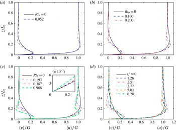
Figure 6(a–c) depicts the separate variations in the mean profiles of
 $u$
and
 $v$
as stability increases for
 $\mathit{Re}_{f}=400$
, 600 and 900, respectively, while figure 6(d) shows the variation of these velocity components with time during one inertial period
 $2{\rm\pi}/f$
(
 $=12\ \text{h}$
) for the case
 $\mathit{Re}_{f}=600$
at
 $\mathit{Ri}_{0,0}=0.002$
. Increasing stability changes the Ekman rotation angle at a given height. It also reduces flow velocities very close to the wall (see inset in figure 6
c), while increasing them away from the wall (see figure 5). This is consistent with the reduced mixing and momentum transport from the upper levels of the boundary layer, where the flow becomes faster, to the near-wall region, where the flow becomes slower, as stability increases. The stable profiles are hence more ‘laminar-like’.
(a–c) Reynolds-averaged non-dimensional velocity profiles at Reynolds number (
 $\mathit{Re}_{f}$
) of (a) 400, (b) 600 and (c) 900 at various stabilities (
 $\mathit{Ri}_{0,0}=0.001$
for
 $\mathit{Re}_{f}=400$
; 0.001, 0.002 for
 $\mathit{Re}_{f}=600$
; and 0.001, 0.002 and 0.005 for
 $\mathit{Re}_{f}=900$
) compared with the neutral case (black solid line in each panel). Corresponding bulk Richardson numbers
 $\mathit{Ri}_{b}$
can be found in table 1 and are shown in the legend of each panel. The inset in panel (c) shows a zoomed-in plot of normalized
 $\langle u\rangle$
near the wall. (d) The time variation of the velocity profiles, averaged over horizontal directions, at
 $\mathit{Re}_{f}=600$
and
 $\mathit{Ri}_{0,0}=0.002$
equivalent to
 $\mathit{Ri}_{b}=0.2$
. Here
 $tf\approx 0$
(solid black lines) shows neutral-case profiles.

The neutral-case turbulent Ekman layer depth can be defined as
 ${\it\delta}_{t}=u_{\ast }/f$
(Caldwell et al.
Reference Caldwell, Van Atta and Helland1972; Coleman et al.
Reference Coleman, Ferziger and Spalart1990; Zilitinkevich & Mironov Reference Zilitinkevich and Mironov1996). As illustrated in table 1, the dimensional friction velocity
 $u_{\ast }$
and, correspondingly, the Ekman layer depth increase with increasing
 $\mathit{Re}$
, and decrease with increasing
 $\mathit{Ri}$
. As the Obukhov length and vertical mixing decrease for the more stable simulations, a shallower boundary layer is produced – a common feature of stable ABLs (Kaimal & Finnigan Reference Kaimal and Finnigan1994). The results obtained here are consistent with this trend. A good indicator of the boundary layer depth is the height at which there is a maximum in the velocity profile; this depth decreases with increasing stability as shown in figure 6. The bands of super-geostrophic velocities around the peaks observed in figures 5 and 6, where the flow speed in the boundary layer can be higher than the geostrophic value far from the wall, are also a common feature seen in stable ABLs (Stull Reference Stull1988).
5.2. Evolution of turbulence and stability
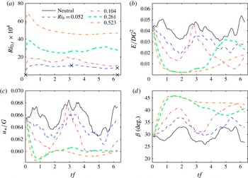
Figures 7(a), 8(a) and 9(a) show the time evolution of the surface Richardson number (
 $\mathit{Ri}_{0,t}=g{\it\Gamma}_{0,t}D^{2}/{\it\theta}_{\infty }G^{2}$
) at various bulk Richardson numbers
 $\mathit{Ri}_{b}=g{\it\delta}_{t}{\rm\Delta}{\it\theta}/{\it\theta}_{0}G^{2}$
, where
 ${\rm\Delta}{\it\theta}={\it\theta}_{\infty }-{\it\theta}_{0}$
. The bulk Richardson number
 $\mathit{Ri}_{b}$
remains almost constant throughout a simulation and we thus use it to characterize the bulk stability. From the plots, it can be seen that the gradient at the surface initially increases, since the initial temperature profiles are not in equilibrium with the turbulent velocity fields; therefore, the gradients at the surface need time to adjust. Subsequently,
 $\mathit{Ri}$
falls back and stabilizes. The cross marks on the plots show the period over which the statistics were averaged (the ones overlaid on the
 $x$
axis are for the neutral cases). Coleman et al. (Reference Coleman, Ferziger and Spalart1992) argue that the first
 $tf=1$
is enough for the development of temperature fluctuations in the field, which would be in equilibrium with the velocity field. However, in our analysis, the time before the first cross mark at
 $tf={\rm\pi}$
is not used for averaging, since during this period the changes in turbulence statistics due to stability seem to remain significant in our simulations. The time interval after
 $tf={\rm\pi}$
has a more or less constant surface Richardson number, confirming that the flow is in quasi-equilibrium and justifying the averaging we perform over this half inertial time period. For the stronger stability simulations at each value of
 $\mathit{Re}$
, intermittency is observed whereby turbulence is damped and then regenerated as discussed previously. This behaviour has also been observed by García-Villalba & Del Álamo (Reference García-Villalba and Del Álamo2011) in their channel flow simulations, and might be indicative of insufficiently large computational domains for the stronger stratification cases. While these intermittent simulations warrant more in-depth analysis to validate their behaviour and potentially analyse it, in this paper, only data from the continuously turbulent simulations will henceforth be analysed.
Results at
 $\mathit{Re}_{f}=400$
. (a) Surface Richardson number (
 $\mathit{Ri}_{0,t}$
) versus non-dimensional time (
 $tf$
) at various stabilities indicated by the legend. Cross marks indicate the start and end times of the averaging period used for calculating means and the averages of budgets for neutral and weakly stable cases. (b) Non-dimensional volume-integrated TKE per unit area (
 $E$
). (c) Friction velocity (
 $u_{\ast }$
) and its variation with time and stability. (d) Variation of the angle (
 ${\it\beta}$
) between the geostrophic wind direction and the surface shear stress direction with time and stability.

Results at
 $\mathit{Re}_{f}=600$
. (a) Surface Richardson number (
 $\mathit{Ri}_{0,t}$
) versus non-dimensional time (
 $tf$
) at various stabilities indicated by the legend. Cross marks indicate the start and end times of the averaging period used for calculating means and the averages of budgets for neutral and weakly stable cases. (b) Non-dimensional volume-integrated TKE per unit area (
 $E$
). (c) Friction velocity (
 $u_{\ast }$
) and its variation with time and stability. (d) Variation of the angle (
 ${\it\beta}$
) between the geostrophic wind direction and the surface shear stress direction with time and stability.

Results at
 $\mathit{Re}_{f}=900$
. (a) Surface Richardson number (
 $\mathit{Ri}_{0,t}$
) versus non-dimensional time (
 $tf$
) at various stabilities indicated by the legend. Cross marks indicate the start and end times of the averaging period used for calculating means and the averages of budgets for neutral and weakly stable cases. For the highest stable stratification imposed, the period denoted by cross marks in panel (a) for
 $\mathit{Ri}_{b}=1.936$
shows the intermittency in that time period and hence has not been used for analysis. (b) Non-dimensional volume-integrated TKE per unit area (
 $E$
). (c) Friction velocity (
 $u_{\ast }$
) and its variation with time and stability. (d) Variation of the angle (
 ${\it\beta}$
) between the geostrophic wind direction and the surface shear stress direction with time and stability.

In figures 7(b), 8(b) and 9(b), we plot the variation of volume-integrated TKE per unit area (
 $E$
), non-dimensionalized by the laminar Ekman layer depth (
 $D$
) and the square of the geostrophic wind velocity (
 $G^{2}$
), versus time, for various stabilities. The volume-integrated TKE (per unit area) averaged over a horizontal plane is defined as
 $$\begin{eqnarray}E=\frac{1}{2}\int _{0}^{L_{z}}\langle u_{i}^{\prime }u_{i}^{\prime }\rangle _{x,y}\text{d}z.\end{eqnarray}$$
Here
 $\langle \;\rangle _{x,y}$
indicates averaging over
 $xy$
planes, the prime (
 $^{\prime }$
) indicates the fluctuating component and
 $L_{z}$
is the top of the domain. The TKE drops down with increasing stability (the mechanisms behind this drop are discussed later in the paper), with most of the drop occurring when the flow transitions from neutral to weakly stable. For Reynolds numbers of 600 and 900, the total TKE in the domain for the least stable cases is about half of that for the neutral simulation. For the highest Richardson numbers imposed at every value of the Reynolds number, the TKE in the domain drops almost to zero, but with strong intermittent bursts. The bulk Richardson number at which this intermittency sets in varies with
 $\mathit{Re}_{f}$
(recall the discussion of the variation of the critical Richardson number with
 $\mathit{Re}$
above). We also observe that the stronger the imposed stability, the faster the rate at which TKE drops at initial times. The decay rates of the TKE near the wall are consistent with a scaling with
 $L/u_{\ast }$
, as reported by Flores & Riley (Reference Flores and Riley2011). Note that all the simulations have the same initial state (fully turbulent neutral Ekman layer), and hence this comparison is meaningful.
Figures 7(c), 8(c) and 9(c) show the evolution of the friction velocity (non-dimensionalized by the geostrophic wind velocity
 $G$
;
 $u_{\ast }/G$
is referred to in the meteorological literature as the geostrophic drag coefficient) versus time. Static stability reduces the friction velocity (and thus the surface momentum flux). The initial rate at which the friction velocity drops from the neutral-case initial value also increases with stability. At large stabilities, there are bursts in the friction velocity too, associated with the turbulent bursts, which increase
 $u_{\ast }$
to values comparable to those seen in the neutral cases. One should note here that, for the neutral and weakly stable simulations,
 $u_{\ast }/G\approx 0.05$
, which is the value used by Monin & Obukhov (Reference Monin and Obukhov1954) to estimate the rate of decrease in fluxes with height discussed above.
Figures 7(d), 8(d) and 9(d) show the variation of the angle between the geostrophic wind velocity vector and the shear stress vector at the surface versus time, for the various stabilities. Note that the angle for the turbulent neutral case is denoted by the black solid lines, while the value of the angle at the surface for the laminar limit is 45° (Stull Reference Stull1988). This limit can be obtained by solving the Reynolds-averaged equations of motion with the simplifying assumptions of steadiness, homogeneity in the horizontal directions, neutral stratification and a constant viscosity. With increasing stability, as the TKE drops and the flow becomes less turbulent, the angle at the surface increases and approaches the limit of 45° for the laminarizing intermittent cases.
The average angle,
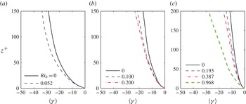
 $\langle {\it\gamma}\rangle$
, between the surface shear stress (which is about aligned with the wind very close to the surface) and the wind direction with height is depicted in figure 10. In many stable boundary layer theories, it is assumed that the turning due to the Coriolis force is negligibly small near the surface (lowest 10 % of the boundary layer). From the plots, it is clear that, even if the direct effect of the Coriolis force is small on turbulence (as compared to other terms in the budgets analysed later), the angle between surface shear stress and wind direction can be significant, particularly at higher stabilities. However,
 $\langle {\it\gamma}\rangle$
decreases with increasing Reynolds number, and thus higher-Reynolds-number simulations will be needed to verify whether
 $\langle {\it\gamma}\rangle$
is indeed negligible in the lower ABL.
Average angle between the shear stress at the surface and the wind velocity,
 $\langle {\it\gamma}\rangle =\tan ^{-1}(v/u)-{\it\beta}$
, as a function of height in the surface layer: (a)
 $\mathit{Re}_{f}=400$
, (b)
 $\mathit{Re}_{f}=600$
and (c)
 $\mathit{Re}_{f}=900$
at various stabilities indicated in the legend.

5.3. Profiles of the gradient Richardson number, TKE and stress
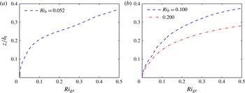
The vertical profiles of the gradient Richardson number are depicted in figure 11. The gradient Richardson number is defined as
 $$\begin{eqnarray}\mathit{Ri}_{gr}=\frac{g}{{\it\theta}_{\infty }}\frac{\text{d}\langle {\it\theta}\rangle /\text{d}z}{(\text{d}\langle u\rangle /\text{d}z)^{2}+(\text{d}\langle v\rangle /\text{d}z)^{2}}.\end{eqnarray}$$
As the Richardson number increases, buoyancy effects will result in complete laminarization of the flow. The exact value at which this happens, called the critical Richardson number (
 $\mathit{Ri}_{c}$
, the value of
 $\mathit{Ri}_{gr}$
below which fluid flow becomes dynamically unstable), is determined by the state of the flow. It has been argued by Miles (Reference Miles1961) and Howard (Reference Howard1961), using linear stability analysis of two-dimensional steady stable shear flows, that a sufficient condition for dynamic stability is that the gradient Richardson number (
 $\mathit{Ri}_{gr}$
) exceed 0.25 everywhere in the flow (any small perturbation will be damped under such conditions). This value of 0.25 is hence often used as an estimate for
 $\mathit{Ri}_{c}$
. However, the limitations of the linear stability analysis and the possibility of sustaining turbulence if the local
 $\mathit{Ri}_{gr}$
is below 0.25 somewhere in the flow makes this estimate not very robust. For example, some studies (see Canuto Reference Canuto2002, and references therein) indicate that
 $\mathit{Ri}_{c}$
may be as large as one or beyond, and some argue that a critical limit does not exist at all (Monin & Yaglom Reference Monin and Yaglom1975; Yamamoto Reference Yamamoto1975; Lettau Reference Lettau1979; Galperin, Sukoriansky & Anderson Reference Galperin, Sukoriansky and Anderson2007). Other arguments suggest that laminarization would happen when the characteristic length of the large eddies (estimated as the Obukhov scale in Flores & Riley (Reference Flores and Riley2011) and the Ozmidov scale in Katul et al. (Reference Katul, Porporato, Shah and Bou-Zeid2014)), which is reduced by buoyancy, approaches some multiple of the Kolmogorov scale, the ratio of the two scales effectively becoming proportional to
 $\mathit{Re}^{3/4}$
. Chung & Matheou (Reference Chung and Matheou2012) also argue in their analysis of stationary homogeneous stratified turbulence that the Richardson number is not sufficient to determine the state of the flow; a measure of the scale separation (given by the Reynolds number) is also needed. This point of view is confirmed by our previous analysis in this paper where we illustrated that the Richardson number at which intermittency starts being observed depends on the Reynolds number.
Gradient Richardson number as a function of height with varying stabilities at a Reynolds number
 $\mathit{Re}_{f}$
of (a) 400 and (b) 600. The normalization depth
 ${\it\delta}_{t}$
for all cases is the depth of the neutral boundary layer at the given Reynolds number.

From the profiles in figure 11, one can see that buoyancy starts influencing the flow significantly (large
 $\mathit{Ri}_{gr}$
exceeding some arbitrary threshold, e.g. 0.25) only at larger heights, but this critical height at which buoyancy becomes important decreases drastically with increasing
 $\mathit{Ri}_{b}$
owing to the decrease of the boundary layer depth. A very similar trend is observed in the plot with
 $\mathit{Re}_{f}=900$
(not shown here), indicating a decrease in the height at which the ‘critical’ Richardson number is reached. Note that the normalization of height (
 $y$
axis here) is carried out using the depth (turbulent length scale) of the neutral simulations. Other scales can be used for normalization (Mironov & Fedorovich (Reference Mironov and Fedorovich2010), for example, pointed to several depth scales for stable boundary layers that are consistent with TKE and momentum budgets), but, to emphasize the effect of static stability on turbulence at a given dimensional distance from the wall, we use the fixed neutral-case turbulent Ekman layer length scale for normalization.
Figure 12 presents the vertical variation of
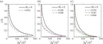
 $2q^{2}=\langle u_{i}^{\prime }u_{i}^{\prime }\rangle$
(twice the TKE) at various stabilities and at different Reynolds numbers. Increasing
 $\mathit{Re}$
brings the peak in
 $2q^{2}$
closer to the wall as expected, while increasing
 $\mathit{Ri}$
generally reduces the peak values of
 $2q^{2}$
; for the highest stabilities, the peaks move slightly away from the wall.
Profiles of the time-averaged non-dimensional sum of the variances of the three velocity components (i.e.
 $2q^{2}$
, where
 $q^{2}$
is TKE) at Reynolds number (
 $\mathit{Re}_{f}$
) of (a) 400 (b) 600 and (c) 900 at various stabilities, compared with the corresponding neutral cases (black solid line in each panel). The bulk Richardson numbers
 $\mathit{Ri}_{b}$
given in the legend correspond, from lowest to highest, to the following initial surface Richardson numbers:
 $\mathit{Ri}_{0,0}=0.001$
, 0.002, 0.005.

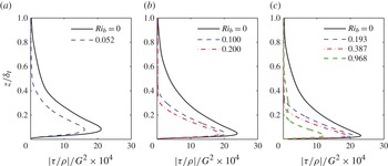
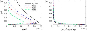
Figure 13 depicts the vertical profiles of the magnitude of the kinematic stress, for various Reynolds numbers and stabilities. The magnitude of this kinematic turbulent stress
 $|{\it\tau}/{\it\rho}|$
is defined as follows:
 $$\begin{eqnarray}|\frac{{\it\tau}}{{\it\rho}}|=(\langle u^{\prime }w^{\prime }\rangle ^{2}+\langle v^{\prime }w^{\prime }\rangle ^{2})^{1/2}.\end{eqnarray}$$
More than for the TKE, the effect of stability on the stress profiles is very pronounced. The stresses (and hence the momentum fluxes) are monotonically damped with increasing stability. This damping of fluxes by buoyancy will be a critical factor in reducing TKE in stable boundary layers, as will be illustrated in the next subsection.
Time-averaged non-dimensional Reynolds stress (
 $|{\it\tau}/{\it\rho}|$
) profiles at
 $\mathit{Re}_{f}$
of (a) 400, (b) 600 and (c) 900 at various stabilities compared with neutral cases. The bulk Richardson numbers
 $\mathit{Ri}_{b}$
given in the legend correspond, from lowest to highest, to the following initial surface Richardson numbers:
 $\mathit{Ri}_{0,0}=0.001$
, 0.002, 0.005.

5.4. TKE and momentum flux budgets
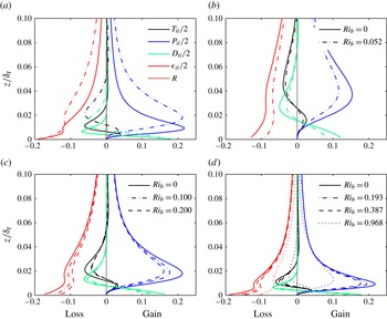
We have seen from vertical profiles of TKE (figure 12) that buoyancy affects turbulence at all heights, but more so away from the wall where the velocity shear is weaker. It has also been observed in the evolution of TKE with time that, as static stability is increased, the total TKE in the domain decreases (figures 7 b, 8 b and 9 b). To investigate the mechanisms causing this reduction in TKE, we study the TKE budgets for stable cases in comparison with neutral ones at the same Reynolds number. Figure 14 shows TKE budgets for all the Reynolds numbers and with varying stabilities.
(a) Turbulence kinetic energy (
 $q^{2}=\langle u_{i}^{\prime }u_{i}^{\prime }\rangle /2$
) budget neutral-case comparison for
 $\mathit{Re}_{f}=600$
(dotted-dashed lines) and
 $\mathit{Re}_{f}=900$
(solid lines); and (b–d) comparison of the neutral case with stable cases at Reynolds numbers (
 $\mathit{Re}_{f}$
) of (b) 400, (c) 600 and (d) 900. Different line styles indicate the various stabilities and different greyscales (colours online) denote the various terms of the budget:
 $\partial q/\partial t+U_{k}(\partial q/\partial x_{k})=(P_{ii}+T_{ii}+{\it\Pi}_{ii}+B_{ii}+C_{ii}+D_{ii}+{\it\epsilon}_{ii})/2$
, where turbulent transport
 $T_{ii}=-\partial \langle u_{i}^{\prime }u_{i}^{\prime }w^{\prime }\rangle /\partial z$
, shear production
 $P_{ii}=-\langle u_{i}^{\prime }w^{\prime }\rangle \partial U_{i}/\partial z$
, viscous diffusion
 $D_{ii}={\it\nu}\partial ^{2}\langle u_{i}^{\prime }u_{i}^{\prime }\rangle /\partial ^{2}z$
and viscous dissipation rate
 ${\it\epsilon}_{ii}=-2{\it\nu}\langle (\partial u_{i}^{\prime }/\partial x_{k})(\partial u_{i}^{\prime }/\partial x_{k})\rangle$
. Note that the computation of the terms is simplified to take advantage of the horizontal homogeneity of the flow and of the zero mean vertical velocity. The terms that are not plotted or shown in the legend have been computed and found to be negligibly small (including the Coriolis term
 $C_{ii}$
, which theoretically is zero), but the full expressions of these terms can be found in appendix C. In panel (a) we plot the residual
 $R$
, which should be zero for validation. We also checked the residuals in non-neutral cases, and they are sufficiently small (but non-zero since the simulations are not exactly in steady state) to validate our computations of the different terms. All terms are normalized by
 $u_{\ast ,neutral}^{4}/{\it\nu}$
. The vertical grey line at the centre of each panel indicates the zero gain/loss line.

Figure 14(a) shows the trends of all the terms in the TKE budget equation for the neutral simulations at Reynolds numbers of
 $\mathit{Re}_{f}$
of 600 and 900. Note that the peaks of the shear production
 $P_{ii}$
, turbulent transport
 $T_{ii}$
and viscous diffusion
 $D_{ii}$
have almost the same value near the wall, after normalization by the relevant velocity scale (friction velocity
 $u_{\ast }$
in this case; see caption of the figure) at both Reynolds numbers. However, the height at which those peaks occur is reduced with increasing Reynolds number, as expected. The vertical trends of all terms are in very good qualitative agreements with the budget computed by Ansorge & Mellado (Reference Ansorge and Mellado2014) (exact quantitative comparison is not possible owing to small differences in the Reynolds number). Figure 14(b–d) compares these terms in neutral and (continuously turbulent) stable cases at
 $\mathit{Re}_{f}=400,\ 600$
and 900, respectively. When stability is imposed, though the overall shapes remain more or less the same, the magnitudes of the individual terms drop. The friction velocity used for non-dimensionalization is the neutral-case value
 $u_{\ast ,neutral}$
at the corresponding Reynolds number, so that the reduction in the budget terms with stability is captured. Normalization based on respective friction velocities for stable cases has been carried out (not shown here), and it was observed that the profiles of the TKE budget terms for
 $\mathit{Re}_{f}=900$
(but not for lower
 $\mathit{Re}_{f}$
) collapse well on to the neutral-case lines, as is observed in the ABL (see Stull Reference Stull1988).
The TKE buoyancy destruction terms are not shown in the TKE budget plots, but are plotted separately in figure 15. The term is very small in comparison to the other terms in the TKE budget, but it is not zero. In fact, one can clearly observe the increase in its magnitude with increasing static stability. This implies that the main direct impact of stability on the flow is not through TKE destruction, but rather through another mechanism: from the plots in figure 14 one can see that a drastic drop in the shear production of TKE is induced by stability. Hence, it is the inhibition of shear production that seems to be the most prominent impact of stability on the TKE budget. This is also in agreement with the conclusions of Ansorge & Mellado (Reference Ansorge and Mellado2014). Since, in a steady turbulence state with small direct buoyant destruction, domain-averaged TKE dissipation has to be approximately equal to TKE production, dissipation is also significantly reduced. Viscous diffusion terms near the wall and turbulent transport, which have smaller contributions in the TKE budget, are similarly decreased.
Profiles of buoyant destruction
 $B_{ii}/2=g\langle w^{\prime }{\it\theta}^{\prime }\rangle /{\it\theta}_{\infty }$
normalized by the viscosity and the neutral-case friction velocity, the same non-dimensionalization used in the TKE budget, at (a)
 $\mathit{Re}_{f}=600$
and (b)
 $\mathit{Re}_{f}=900$
.

To elucidate the mechanism and causes of the drop in shear TKE production, we investigate the quantities involved in this term, namely the gradients and fluxes. The fluxes (
 $\langle u^{\prime }w^{\prime }\rangle ,\langle v^{\prime }w^{\prime }\rangle$
) and the gradients (
 $\partial \langle u\rangle /\partial z,\partial \langle v\rangle /\partial z$
) that enter in the two dominant terms of the TKE shear production,
 $$\begin{eqnarray}-\langle u^{\prime }w^{\prime }\rangle \frac{\partial \langle u\rangle }{\partial z}\quad \text{and}\quad -\langle v^{\prime }w^{\prime }\rangle \frac{\partial \langle v\rangle }{\partial z},\end{eqnarray}$$
are plotted in figure 16 for
 $\mathit{Re}_{f}=900$
. The effect of stability on velocity gradients near the wall is significant, while away from the wall, this effect is reduced. In general, gradients are reduced near the wall by a factor of approximately 2 and increased away from the wall, with higher gradients for the more stable conditions at heights where peaks in the TKE production are seen. Changes in gradients thus cannot explain the sharp drops in TKE production. The effect of stability on the Reynolds stresses (
 $=-\text{vertical momentum fluxes}$
), however, is much more significant. The fluxes are reduced due to static stability throughout the boundary layer compared to the neutral case. This indicates that the reduction due to stability in the vertical transport of momentum from the higher elevations in the boundary layer into the near-wall region, where shear production can occur, is the main mechanism for the reduction in this TKE production term in stable wall-bounded flows.
(a) Magnitude of turbulent stress
 ${\it\tau}=(\langle u^{\prime }w^{\prime }\rangle ^{2}+\langle v^{\prime }w^{\prime }\rangle ^{2})^{1/2}$
and (b) magnitude of the viscous stress
 ${\it\nu}|\langle \text{d}\boldsymbol{u}/\text{d}z\rangle |$
, which represents the gradients (where
 $|\langle \text{d}\boldsymbol{u}/\text{d}z\rangle |=(\langle \text{d}u/\text{d}z\rangle ^{2}+\langle \text{d}v/\text{d}z\rangle ^{2})^{1/2}$
), at
 $\mathit{Re}_{f}=900$
.

The normalization used in figure 16 also makes the gradients plotted in panel (b) equivalent to viscous stresses, normalized by
 $G^{2}$
, while panel (a) depicts the turbulent stresses also normalized by
 $G^{2}$
. Hence from this figure one can compare the viscous and turbulent stresses and observe the increase in the relative importance of the turbulent part as the distance to the wall increases, and as stability decreases.
To further understand the reduction of the momentum fluxes by buoyancy, we study the momentum flux budgets for
 $\langle u^{\prime }w^{\prime }\rangle$
(the
 $\langle v^{\prime }w^{\prime }\rangle$
budget was computed but is not shown here since the behaviour is very similar to the
 $\langle u^{\prime }w^{\prime }\rangle$
budget). Figure 17(a) shows all the terms of the flux budget for the neutral case with
 $\mathit{Re}_{f}=900$
. Details of the equations for the flux budgets and all the terms in it can be found in appendix C. For clarity, only the significant terms have been plotted in figure 17(b–d), where the effects of stability are illustrated. Note that, since the flux is negative, sources would be negative and sinks positive. As seen in the TKE budget plots, the peaks in vertical profiles shift towards the wall with increasing Reynolds numbers. The magnitudes of the peak values also increase with Reynolds number, even though each budget is normalized with the neutral friction velocity at its corresponding Reynolds number. The figure illustrates that the pressure correlation and return to isotropy terms, which have opposite signs near the surface, are both reduced in magnitude as stability increases; the changes in these terms near the surface for stronger stabilities partially offset each other. The flux production (which like the TKE shear production depends on the fluxes themselves) and the turbulent transport terms are also significantly damped by buoyancy. Given that the highest gradients are in the vertical direction, the dominant components of these terms will be
 $-\partial \langle u^{\prime }w^{\prime }w^{\prime }\rangle /\partial z$
in the transport and
 $-\langle w^{\prime }w^{\prime }\rangle \partial U/\partial z$
in the production, both of which are strongly dependent on
 $w^{\prime }$
. Therefore, damping of turbulent transport of momentum, which as we showed leads to a reduction in TKE, seems to be a result of the damping of
 $w^{\prime 2}$
, which is a component of the TKE. This circular dependence thus needs further elucidation. Note that the buoyancy term
 $B_{13}$
here remains much smaller than the other components.
(a) Momentum flux (
 $\langle u^{\prime }w^{\prime }\rangle$
) budget for the neutral case at
 $\mathit{Re}_{f}=900$
, and (b–d) comparison of neutral and stable cases at Reynolds numbers (
 $\mathit{Re}_{f}$
) of (b) 400, (c) 600 and (d) 900. Different line styles indicate the various stabilities and different greyscales (colours online) denote the various terms of the budget:
 $\partial \langle u^{\prime }w^{\prime }\rangle /\partial t+U_{k}(\partial \langle u^{\prime }w^{\prime }\rangle /\partial x_{k})=P_{13}+T_{13}+C_{13}+D_{13}+{\it\Pi}_{13}+{\it\phi}_{13}+{\it\epsilon}_{13}+B_{13}$
, where turbulent transport
 $T_{13}=-\partial \langle u^{\prime }w^{\prime }w^{\prime }\rangle /\partial z$
, turbulent production
 $P_{13}=-\langle w^{\prime }w^{\prime }\rangle \partial U/\partial z$
, pressure transport
 ${\it\Pi}_{13}=-(1/{\it\rho}_{\infty })(\partial \langle p^{\prime }u^{\prime }\rangle /\partial z+\partial \langle p^{\prime }w^{\prime }\rangle /\partial x)$
, pressure–strain redistribution
 ${\it\phi}=(2/{\it\rho}_{\infty })\langle p^{\prime }S_{13}^{\prime }\rangle$
with strain-rate tensor
 $\mathsf{S}_{ij}=[\partial u_{i}/\partial x_{j}+\partial u_{j}/\partial x_{i}]/2$
, molecular diffusion
 $D_{13}={\it\nu}\partial ^{2}\langle u^{\prime }w^{\prime }\rangle /\partial ^{2}z$
, viscous dissipation
 ${\it\epsilon}_{13}=-2{\it\nu}\langle (\partial u^{\prime }/\partial x_{k})(\partial w^{\prime }/\partial x_{k})\rangle$
, and buoyancy
 $B_{13}=g\langle u^{\prime }{\it\theta}^{\prime }\rangle /{\it\theta}_{\infty }$
. All terms are normalized by
 $u_{\ast ,neutral}^{4}/{\it\nu}$
. The vertical grey line at the centre of each panel indicates the zero gain/loss line, but note that here sources would be negative since the momentum flux is negative. The computation of the terms is simplified to take advantage of the horizontal homogeneity of the flow and of the zero mean vertical velocity. Full budget equations can be found in appendix C.

To clarify the sequence of effects that stability induces in a turbulent boundary layer, we now plot the budget of the vertical velocity variance (figure 18). The plot in figure 18(a) compares the budget of vertical velocity variance in the neutral case to the case with stability at
 $\mathit{Ri}_{0,0}=0.002$
for Reynolds number
 $\mathit{Re}_{f}=600$
, while figure 18(b) gives the same comparison at
 $\mathit{Re}_{f}=900$
and
 $\mathit{Ri}_{0,0}=0.005$
. It is observed from the plots that the change in the buoyancy destruction here, while still small, is of the same order as the changes in the other terms. For example, the drop in the peak of the pressure redistribution term, which is the main source in this budget, from the neutral to the most stable simulation at
 $\mathit{Re}_{f}=900$
is only 2.5 times the increase in buoyancy destruction. Notice that we are comparing the change in the terms from neutral to stable simulations, not their magnitude (for the neutral case this buoyancy destruction is zero). This is thus the only budget where the direct effect of buoyancy, via a destruction term, is significant. This implies that buoyancy first affects motions in the vertical direction, damping
 $w^{\prime }$
and
 $\langle w^{\prime }w^{\prime }\rangle$
, which then causes a reduction in the production, and hence in the magnitude, of the momentum fluxes (
 $\langle u^{\prime }w^{\prime }\rangle$
and
 $\langle v^{\prime }w^{\prime }\rangle$
), which then leads to lower TKE production, particularly of the
 $\langle u^{\prime 2}\rangle$
and
 $\langle v^{\prime 2}\rangle$
components of the TKE (the shear production of
 $\langle w^{\prime 2}\rangle$
is zero since it involves gradients of the mean vertical velocity). The reduction in
 $\langle u^{\prime 2}\rangle$
and
 $\langle v^{\prime 2}\rangle$
could then lead to the reduction in the pressure–strain redistribution term illustrated in figure 18, further reducing
 $\langle w^{\prime 2}\rangle$
, but more in-depth analysis of the impact of buoyancy on this redistribution term is needed to ascertain that. We also analysed the turbulent transport efficiencies estimated via
 $R_{uw}=\langle u^{\prime }w^{\prime }\rangle /{\it\sigma}_{u}{\it\sigma}_{w}$
and
 $R_{vw}=\langle v^{\prime }w^{\prime }\rangle /{\it\sigma}_{v}{\it\sigma}_{w}$
, and, while they decrease with increasing stability away from the wall, near the wall they remain about constant. This confirms that the reduction in the momentum fluxes is related to a drop in the amplitude of the vertical velocity, rather than to a drop in the turbulent transport efficiency.
Comparison of budgets of the variance of vertical velocity (
 $\langle w^{\prime }w^{\prime }\rangle$
) for neutral case with stable cases: (a)
 $\mathit{Re}_{f}=600$
, where solid line corresponds to neutral case and dashed line corresponds to stable case with
 $\mathit{Ri}_{b}=0.200$
; (b)
 $\mathit{Re}_{f}=900$
, where solid line corresponds to neutral case and dashed line corresponds to stable case with
 $\mathit{Ri}_{b}=0.968$
. Different line styles indicate the various stabilities and different greyscales (colours online) denote the various terms of the budget:
 $\partial \langle w^{\prime }w^{\prime }\rangle /\partial t+U_{k}(\partial \langle w^{\prime }w^{\prime }\rangle /\partial x_{k})=P_{33}+T_{33}+C_{33}+D_{33}+{\it\Pi}_{33}+{\it\phi}_{33}+{\it\epsilon}_{33}+B_{33}$
, where turbulent transport
 $T_{33}=-\partial \langle w^{\prime }w^{\prime }w^{\prime }\rangle /\partial z$
, pressure transport
 ${\it\Pi}_{33}=(-2/{\it\rho}_{\infty })\ \partial \langle p^{\prime }w^{\prime }\rangle /\partial z$
, pressure–strain redistribution
 ${\it\Phi}_{33}=(2/{\it\rho}_{\infty })\langle p^{\prime }S_{33}^{\prime }\rangle$
with strain-rate tensor
 $\mathsf{S}_{ij}=[\partial u_{i}/\partial x_{j}+\partial u_{j}/\partial x_{i}]/2$
, viscous diffusion
 $D_{33}={\it\nu}\partial ^{2}\langle w^{\prime }w^{\prime }\rangle /\partial ^{2}z$
, viscous dissipation rate
 ${\it\epsilon}_{33}=-2{\it\nu}\langle (\partial w^{\prime }/\partial x_{k})(\partial w^{\prime }/\partial x_{k})\rangle$
and buoyancy destruction
 $B_{33}=2(g/{\it\theta}_{\infty })\langle w^{\prime }{\it\theta}^{\prime }\rangle$
. All terms are normalized by
 $u_{\ast ,neutral}^{4}/{\it\nu}$
; minor terms including production, are not shown. The vertical grey line at the centre of each panel indicates the zero gain/loss line. The computation of the terms is simplified to take advantage of the horizontal homogeneity of the flow and of the zero mean vertical velocity. Full budget equations can be found in appendix C.

Figure 19 shows the profiles of the horizontal velocity variance (a) and the vertical velocity variance (b), illustrating that the reduction in
 $\langle w^{\prime 2}\rangle$
relative to the neutral case, which is associated with the damping of the vertical motions, is larger than the relative reduction in
 $\langle u^{\prime 2}\rangle$
and
 $\langle v^{\prime 2}\rangle$
, as can be anticipated. A particularly important implication of this finding is that even a small Richardson number associated with a small direct buoyant TKE destruction, compared to shear production, can have a significant impact on turbulence in wall-bounded flows: this small TKE destruction will primarily reduce the vertical variance, which then drastically reduces production compared to a neutral flow. This might explain the very rapid drop in TKE levels shortly after the evening transition in the ABL (Nadeau et al.
Reference Nadeau, Pardyjak, Higgins, Fernando and Parlange2011). It is also worth underlining that the reduction in momentum flux under stable conditions results in a reduction in the surface drag. In a pipe or channel flow, this might not be possible if the wall drag needs to balance a fixed imposed pressure gradient. But in an Ekman boundary layer, this is always possible since it just entails a rebalancing of the equilibrium between the pressure gradient, Coriolis and surface drag forces in such a way that the Coriolis force increases and compensates for the reduced surface drag in this equilibrium.
Reduction in the sum of the horizontal velocities variances (a) compared to the reduction in the vertical velocity variance (b) with increasing static stability at
 $\mathit{Re}_{f}=900$
. The black solid line corresponds to the neutral case; and other lines correspond to stable cases: dashed line (blue online)
 $\mathit{Ri}_{b}=0.193$
and dash-dotted line (red online)
 $\mathit{Ri}_{b}=0.387$
.

5.5. Buoyancy flux and temperature variance budgets
Heat flux budgets for all the stable cases are shown in figure 20. The shear production of heat flux given by
 $P^{2}=-\langle {\it\theta}^{\prime }u_{j}^{\prime }\rangle \,\partial \langle w\rangle /\partial x_{j}$
is identically zero for the flows simulated here. The main source of covariance or flux is the production term with temperature gradient
 $P^{1}=-\langle w^{\prime }u_{j}^{\prime }\rangle \,\partial \langle {\it\theta}\rangle /\partial x_{j}$
(note that production and other sources here are negative since the heat flux is negative or downwards; in a statically unstable boundary layer it would be positive). The two significant terms are the pressure terms, while other terms (namely the Coriolis term
 $C$
, dissipation
 ${\it\epsilon}_{23}$
, viscous diffusion
 $D_{23}$
and turbulent transport
 $T_{23}$
) are quite small for neutral simulations. For simulations with stable stratification, the reduction in the temperature gradient production term drives the buoyancy effect on this budget. However, the buoyancy destruction term becomes important at stronger stabilities, especially for the
 $\mathit{Re}_{f}=900$
simulation. Note here that, for increasing stabilities, the vertical temperature gradient is larger in magnitude, and yet the gradient production term is smaller. This results from the significant drop in the magnitude of the variance of the
 $w$
component of velocity with stability, illustrated in the previous subsection, which appears in this production term. Expressions for all the terms involved in the heat flux budget can be found in appendix C.
(a) Buoyancy flux (
 $\langle w^{\prime }{\it\theta}^{\prime }\rangle$
) budget for the stable case at
 $\mathit{Re}_{f}=900$
,
 $\mathit{Ri}_{0,0}=0.001$
and (b–d) comparison of all significant terms from the stable cases at Reynolds numbers (
 $\mathit{Re}_{f}$
) of (b) 400, (c) 600 and (d) 900. Different line styles indicate the various stabilities and different greyscales (colours online) denote the various terms of the budget:
 $\partial \langle w^{\prime }{\it\theta}^{\prime }\rangle /\partial t+U_{j}(\partial \langle w^{\prime }{\it\theta}^{\prime }\rangle /\partial x_{j})=P^{1}+P^{2}+T+{\it\Pi}+{\it\phi}+D^{1}+D^{2}+{\it\chi}+B$
, where turbulent production by mean temperature gradient
 $P^{1}=-\langle w^{\prime }w^{\prime }\rangle \partial \langle {\it\theta}\rangle /\partial z$
, buoyancy destruction
 $B=g\langle {\it\theta}^{\prime }{\it\theta}^{\prime }\rangle /{\it\theta}_{\infty }$
, turbulent transport
 $T=-\partial \langle w^{\prime }w^{\prime }{\it\theta}^{\prime }\rangle /\partial z$
, transport by pressure correlation
 ${\it\Pi}=-(1/{\it\rho}_{\infty })\partial \langle p^{\prime }{\it\theta}^{\prime }\rangle /\partial z$
, redistribution by return-to-isotropy term
 ${\it\phi}=(1/{\it\rho}_{\infty })\langle p^{\prime }\partial {\it\theta}^{\prime }/\partial z\rangle$
, diffusion by velocity gradients
 $D^{1}=(\partial /\partial z)({\it\nu}\partial \langle {\it\theta}^{\prime }\partial w^{\prime }/\partial z\rangle )$
, diffusion by temperature gradients
 $D^{2}=(\partial /\partial z)({\it\nu}_{{\it\theta}}\partial \langle w^{\prime }\partial {\it\theta}^{\prime }/\partial z\rangle )$
, and molecular dissipation
 ${\it\chi}=-({\it\nu}+{\it\nu}_{{\it\theta}})\langle (\partial w^{\prime }/\partial x_{j})(\partial {\it\theta}^{\prime }/\partial x_{j})\rangle$
. All terms are normalized by
 $u_{\ast ,neutral}^{3}({\it\theta}_{\infty }-{\it\theta}_{0})/{\it\nu}$
. The vertical grey line at the centre of each panel indicates the zero gain/loss line, but note that here sources would be negative since the buoyancy flux is negative in a stable boundary layer. The computation of the terms is simplified to take advantage of the horizontal homogeneity of the flow and of the zero mean vertical velocity. Full budget equations can be found in appendix C.

The last budget we examine is the budget of the perturbation temperature variance (
 $\langle {\it\theta}^{\prime }{\it\theta}^{\prime }\rangle$
) plotted in figure 21. Similar to TKE budget plots, from these plots one can infer that the main terms being modified by stability are the variance production terms. Variance dissipation falls with decreasing production. Turbulent transport and molecular diffusion away from the wall are small, while near the wall they are very weakly affected by buoyancy.
(a) Temperature variance (
 $\langle {\it\theta}^{\prime }{\it\theta}^{\prime }\rangle$
) budget at
 $\mathit{Re}_{f}=900$
and
 $\mathit{Ri}_{0,0}=0.001$
and (b–d) comparison of all the significant terms from the stable cases at Reynolds numbers (
 $\mathit{Re}_{f}$
) of (b) 400, (c) 600 and (d) 900 and at various Richardson numbers. Different line styles indicate the various stabilities and different greyscales (colours online) denote the various terms of the budget:
 $\partial \langle {\it\theta}^{\prime }{\it\theta}^{\prime }\rangle /\partial t+U_{j}(\partial \langle {\it\theta}^{\prime }{\it\theta}^{\prime }\rangle /\partial x_{j})=P_{{\it\theta}}+T_{{\it\theta}}+D_{{\it\theta}}+{\it\chi}_{{\it\theta}}$
, where production
 $P_{{\it\theta}}=-2\langle w^{\prime }{\it\theta}^{\prime }\rangle \partial \langle {\it\theta}\rangle /\partial z$
, turbulent transport
 $T_{{\it\theta}}=-\partial \langle w^{\prime }{\it\theta}^{\prime }{\it\theta}^{\prime }\rangle /\partial z$
, molecular diffusion
 $D_{{\it\theta}}={\it\nu}_{{\it\theta}}\partial ^{2}\langle {\it\theta}^{\prime }{\it\theta}^{\prime }\rangle /\partial ^{2}z$
, and molecular dissipation
 ${\it\epsilon}_{{\it\theta}}=-2{\it\nu}_{{\it\theta}}\langle (\partial {\it\theta}^{\prime }/\partial x_{j})(\partial {\it\theta}^{\prime }/\partial x_{j})\rangle$
. All terms are normalized by
 $u_{\ast ,neutral}^{2}({\it\theta}_{\infty }-{\it\theta}_{0})^{2}/({\it\nu}/\mathit{Pr})$
. The vertical grey line at the centre of each panel indicates the zero gain/loss line. The computation of the terms is simplified to take advantage of the horizontal homogeneity of the flow and of the zero mean vertical velocity. Full budget equations can be found in appendix C.

5.6. Turbulent diffusivities under stable conditions
Most stable flows of practical engineering or geophysical relevance are at much higher Reynolds numbers than the ones we can attain here, and many can only be modelled using the Reynolds-averaged Navier–Stokes (RANS) approach (e.g. stable ABL in weather and climate models). Thus, an important follow-up on the investigation of turbulence dynamics and budgets that we performed in the previous sections is to relate the findings to the development of better turbulence closure models for stable conditions and the comparison to existing models for very high-
 $\mathit{Re}$
flows. Readers interested in higher-order closures will find the detailed budget analyses very useful for supporting simplifications of the budget equations that are explicitly solved in models and for guiding the development of such closures. A large fraction of weather and climate models, however, continue to rely on simple first-order or 1.5-order closures under stable conditions; therefore, we focus in this section on the eddy diffusivities and viscosities needed for these closures. We do not aim to develop new closures, but rather to test the assumptions underlying existing ones.
Figure 22 shows the vertical profiles of eddy viscosity (
 ${\it\nu}_{T}$
) and eddy diffusivity (
 ${\it\alpha}_{T}$
) for
 $\mathit{Re}_{f}$
of 400, 600 and 900, non-dimensionalized by molecular viscosity and diffusivity. Following Coleman et al. (Reference Coleman, Ferziger and Spalart1992), eddy viscosity and diffusivity are computed using the following relations:
 $$\begin{eqnarray}\displaystyle & \displaystyle {\it\nu}_{T}=\frac{-\langle u^{\prime }w^{\prime }\rangle \,\text{d}\langle u\rangle /\text{d}z-\langle v^{\prime }w^{\prime }\rangle \,\text{d}\langle v\rangle /\text{d}z}{(\text{d}\langle u\rangle /\text{d}z)^{2}+(\text{d}\langle v\rangle /\text{d}z)^{2}}, & \displaystyle\end{eqnarray}$$
 $$\begin{eqnarray}\displaystyle & \displaystyle {\it\alpha}_{T}=\frac{-\langle w^{\prime }{\it\theta}^{\prime }\rangle }{\text{d}\langle {\it\theta}\rangle /\text{d}z}. & \displaystyle\end{eqnarray}$$
Profiles of (a,c,e) eddy viscosity and (b,d, f) eddy diffusivity non-dimensionalized by their molecular counterparts under varying stabilities for
 $\mathit{Re}_{f}$
of (a,b) 400, (c,d) 600 and (e, f) 900.

In figure 23, we plot the vertical eddy viscosities evaluated separately for the
 $x$
and
 $y$
momentum components (
 ${\it\nu}_{Tx}=-\langle u^{\prime }w^{\prime }\rangle /(\text{d}\langle u\rangle /\text{d}z)$
and
 ${\it\nu}_{Ty}=-\langle v^{\prime }w^{\prime }\rangle /(\text{d}\langle v\rangle /\text{d}z)$
) to test the assumption that the eddy viscosity is isotropic (hence a scalar, see Smagorinsky (Reference Smagorinsky1963), for example), which follows from the Boussinesq analogy. Note that the results are plotted only for values of
 $z/L_{z}$
(
 $L_{z}$
is the domain height) less than 0.2 and where
 $\text{d}\langle v\rangle /\text{d}z$
is not close to zero. From the plots, it seems that this assumption is not exactly applicable: the eddy viscosity evaluated in the
 $y$
direction,
 ${\it\nu}_{Ty}$
, is consistently smaller than that evaluated in the
 $x$
direction,
 ${\it\nu}_{Tx}$
. However, one must note that the discrepancy between the two viscosities seems to be reduced at higher Reynolds numbers and also at higher Richardson numbers. These trends are in agreement with the LES results of Huang, Bou-Zeid & Golaz (Reference Huang, Bou-Zeid and Golaz2013) (at much higher Reynolds numbers), who showed that the Boussinesq analogy was reasonable and its applicability in fact improved with increasing stability. Assuming equality of the two viscosities is equivalent to hypothesizing that the fluxes and gradients or strains are aligned. Plots not shown here of the difference between the angles of the stress (
 $\tan ^{-1}(\langle v^{\prime }w^{\prime }\rangle /\langle u^{\prime }w^{\prime }\rangle )$
) and the gradient (
 $\tan ^{-1}(\partial \langle v\rangle /\partial z)/(\partial \langle u\rangle /\partial z)$
) also show improved alignment at higher Reynolds numbers (the angle differences are less than 16° for
 $\mathit{Re}_{f}=600$
and less than 10° for
 $\mathit{Re}_{f}=900$
). These angles are much larger than the ones observed in the wall-modelled LES of Huang et al. (Reference Huang, Bou-Zeid and Golaz2013), again suggesting a Reynolds-number dependence despite the uncertainty in defining the effective Reynolds number in wall-modelled LES.
Profiles of the vertical eddy viscosity for the
 $x$
and
 $y$
momentum components calculated separately (
 ${\it\nu}_{Tx}=-\langle u^{\prime }w^{\prime }\rangle /(\text{d}\langle u\rangle /\text{d}z)$
and
 ${\it\nu}_{Ty}=-\langle v^{\prime }w^{\prime }\rangle /(\text{d}\langle v\rangle /\text{d}z)$
) non-dimensionalized by their molecular counterparts under varying stabilities for
 $\mathit{Re}_{f}$
of (a) 600 and (b) 900. Missing parts in the vertical profiles for the
 $y$
momentum component correspond to layers where the gradients of
 $v$
have near-zero values, resulting in very large viscosities, and hence not shown.

The ratio of
 ${\it\nu}_{T}$
over
 ${\it\alpha}_{T}$
gives the turbulent Prandtl number
 $\mathit{Pr}_{T}={\it\nu}_{T}/{\it\alpha}_{T}$
, which is plotted in figure 24 for all the Reynolds numbers simulated here, at Richardson numbers of
 $\mathit{Ri}_{0,0}=0.001$
and 0.002 (only 0.001 for the lower
 $\mathit{Re}_{f}$
) versus height (panels (a,c,e)) and versus the gradient Richardson number
 $\mathit{Ri}_{gr}$
(panels (b,d, f)). The turbulent Prandtl number increases, but very slightly, with increasing stability (
 $\mathit{Ri}_{0,0}$
), approaching unity. This indicates that buoyancy affects turbulent transfer of heat and momentum in the same way in statically stable flows. This has also been observed by Coleman et al. (Reference Coleman, Ferziger and Spalart1992). However, for higher Reynolds number, several studies suggest that the turbulent Prandtl number increases more significantly with increasing stability (Bou-Zeid et al.
Reference Bou-Zeid, Higgins, Huwald, Meneveau and Parlange2010; Venayagamoorthy & Stretch Reference Venayagamoorthy and Stretch2010; Huang & Bou-Zeid Reference Huang and Bou-Zeid2013). Despite this divergence on the effect of stability on the similarity of momentum and scalar turbulent transport, a robust conclusion from all those studies is that the Reynolds analogy holds much better in stable wall-bounded flows than in unstable (convective) ones (Li et al.
Reference Li, Katul and Bou-Zeid2012; Katul et al.
Reference Katul, Li, Chamecki and Bou-Zeid2013). Therefore, a first-order closure seems to be more acceptable under stable conditions.
Turbulent Prandtl number (
 $\mathit{Pr}_{t}$
) variation with height and with gradient Richardson number (
 $\mathit{Ri}_{gr}$
) at Reynolds numbers (a,b) 400, (c,d) 600 and (e, f) 900.

Figure 25(a,c,e) depicts the ratio of the magnitude of the horizontal Reynolds stress to the square of the vertical velocity variance (which is defined as
 $b_{1}$
in the caption of the figure), with varying stabilities and Reynolds numbers, as a function of height (we only plot heights above the near-wall region where viscous stresses dominate since this analysis is not meaningful there). Figure 25(b,d, f) depicts the ratio of the same stress component to twice the TKE (defined as
 $a_{1}$
in the caption of the figure), again with varying Richardson and Reynolds numbers, as a function of height. These quantities represent measures of turbulent transport efficiencies in the stable boundary layer. One can observe that these fluxes, when non-dimensionalized by the vertical velocity variance, collapse very well onto a single curve in the surface layer (log or MOST layer, roughly where
 $z/{\it\delta}_{t}<0.2$
), except for some discrepancy for the most stable simulation at the highest
 $\mathit{Re}_{f}$
. The ratio
 $b_{1}$
is not very sensitive to stability in the surface layer since both the numerator and denominator decrease proportionally. A reduction in
 $b_{1}$
can be noted at larger heights, indicating that turbulent transport becomes less efficient with increasing stability. However, when non-dimensionalized with TKE, the lines do not collapse anywhere and this measure of efficiency drops down significantly with increasing stability. Horizontal variances are not reduced significantly by stability (thus the preponderance of pancake-like structures in the stable ABL (Beckers et al.
Reference Beckers, Verzicco, Clercx and Van Heijst2001; Riley & de Bruyn Kops Reference Riley and de Bruyn Kops2003; Davidson Reference Davidson2004)) and hence the TKE decreases with stability at a lower rate than vertical fluxes. These results reconfirm that the variance of the vertical velocity is the primary component of the TKE that accounts for vertical fluxes and suggest that 1.5-order closure models should solve the budget equation of the vertical velocity variance, rather than TKE, or use that variance as the basis for formulating vertical eddy viscosities and diffusivities in stable wall-bounded flows. However, solving the equation for the vertical variance can pose some challenges, particularly ones related to the closure of the pressure redistribution term, and this might explain why currently most formulations rely on the full TKE as the basis for eddy viscosity and diffusivity models.
Ratio of the Reynolds stress magnitude to vertical velocity variance,
 $b_{1}$
, at
 $\mathit{Re}_{f}$
of (a) 400, (c) 600 and (e) 900, respectively, and ratio of Reynolds stress magnitude to twice the TKE,
 $a_{1}$
, at
 $\mathit{Re}_{f}$
of (b) 400, (d) 600 and ( f) 900, respectively, as a function of height and bulk Richardson number, where
 $b_{1}=(\langle u^{\prime }w^{\prime }\rangle ^{2}+\langle v^{\prime }w^{\prime }\rangle ^{2})^{1/2}/{\it\sigma}_{w}^{2}$
and
 $a_{1}=(\langle u^{\prime }w^{\prime }\rangle ^{2}+\langle v^{\prime }w^{\prime }\rangle ^{2})^{1/2}/2q^{2}$
with
 $2q^{2}=\langle u_{i}^{\prime }u_{i}^{\prime }\rangle$
and
 ${\it\sigma}_{w}^{2}=\langle w^{\prime }w^{\prime }\rangle$
. We only plot for
 $z/{\it\delta}_{t}>0.05$
, where
 ${\it\delta}_{t}$
is the turbulent boundary layer depth of each simulation, to focus on the regions where the total fluxes are not dominated by the viscous contributions.

6. Conclusions
Direct numerical simulations of neutral and statically stable turbulent Ekman layers were performed at three moderate Reynolds numbers. For cases with stable stratification, a constant surface temperature was imposed at the wall, which resulted in a time-dependent heat flux across the boundary layer; however, analyses are based on periods during which a quasi-equilibrium state has been reached. The results are first compared with experimental and other numerical simulations by plotting the mean profiles of velocity at the same Reynolds numbers. The spectra of temperature and of each of the three components of velocity are also plotted to confirm the development of an inertial range at the highest Reynolds numbers. Non-dimensionalization of spectra using Monin–Obukhov parameters resulted in collapse of the curves in the inertial subrange (premultiplied by
 $k_{x}$
, where
 $k_{x}$
is the streamwise wavenumber) on to a
 $-\frac{2}{3}$
power law as expected. Spectral characteristics at lower wavenumbers are very similar to those seen in the atmosphere under comparable stabilities, despite a small inertial range.
The agreement of the mean profiles with the MOST for the two highest Reynolds numbers simulated (the lowest one displayed no log layer or inertial subrange under neutral conditions) is found to be good, supporting the applicability of that theory in moderately stable wall-bounded flows. However, the empirical constant
 ${\it\beta}_{m}$
in the non-dimensional gradients that was obtained at
 $\mathit{Re}_{f}=600$
and
 $\mathit{Re}_{f}=900$
is approximately equal to 9, suggesting that viscous effects increase
 ${\it\beta}_{m}$
at low to moderate Reynolds numbers, as has been argued by Chung & Matheou (Reference Chung and Matheou2012). Furthermore, the constant flux layer is found to span only the lowest 5 % of the neutral boundary layer when the original criterion used by Monin & Obukhov (Reference Monin and Obukhov1954) of a change of no more than 20 % compared to the surface fluxes is used, and this depth of the constant flux layer is further reduced with increasing stability. Mean profiles of velocity under stably stratified turbulent cases are similar to the ones seen in laminar Ekman layers. A super-geostrophic maximum in the magnitude of the horizontal velocity at a certain height away from the wall is reached (super-geostrophic velocities), and that height decreases with increasing stability. Friction velocity and hence the turbulent Ekman boundary layer height scale (
 ${\it\delta}_{t}=u_{\ast }/f$
) increase with increasing Reynolds number, and decrease with increasing Richardson number.
The total TKE levels in the domain for the weakest stabilities simulated are about half the levels for the corresponding neutral simulation at the same Reynolds number. The stronger the imposed stability, the faster is the rate at which TKE drops at initial times as the flow adjusts from the initial neutral state to the statically stable state. Similar trends are seen in surface momentum flux (friction velocity) plots. With increasing stability, as the TKE drops and the flow becomes less turbulent, the angle (
 ${\it\beta}$
) between the geostrophic wind direction and the surface shear stress direction increases and approaches the laminar limit of 45°. For the strongest stabilities simulated at each Reynolds number, the TKE drops almost to zero, and the friction velocity decreases even further. However, intermittent bursts of turbulence are observed for these highly stable flow cases. This intermittency is also seen in plots of the surface Richardson number and the angle
 ${\it\beta}$
between the surface shear stress and the geostrophic wind velocity. In these cases, turbulence is almost completely damped and then regenerated due to build-up of shear away from the wall. The bulk Richardson number at which this type of intermittency sets in increases with increasing Reynolds number. Given some uncertainty about the adequacy of the size of the domain in representing these intermittent flows, the statistical analyses in the paper focus on the less stable continuously turbulent simulations.
A detailed analysis of several budgets of second-order quantities was conducted. The results suggest that the most significant effect of buoyancy on TKE in the Ekman boundary layer is not through direct destruction. Buoyancy first damps
 $w^{\prime }$
and reduces its variance, which then causes a reduction in the production and consequently in the magnitude of the downward momentum fluxes
 $\langle u^{\prime }w^{\prime }\rangle$
and
 $\langle v^{\prime }w^{\prime }\rangle$
. The damping of the momentum fluxes then reduces TKE production, thus reducing TKE levels with increasing Richardson number. This indirect effect of buoyancy (since the potential temperature does not enter into the TKE shear production term, although it enters in its budget) is significant and has a much larger impact on the TKE budget than direct buoyancy destruction. This finding indicates that stability parameters formulated to describe the balance between shear production and direct buoyant destruction of TKE, such as the flux Richardson number or the Monin–Obukhov stability parameter, might not be sufficient to describe the dynamics of stable Ekman layers. In the normalized TKE budget equation that gives rise to these parameters (e.g. ignoring transport in the TKE budget equation of figure 14 and dividing by
 $P_{ii}$
yields
 $P_{ii}^{-1}Dq/Dt=1+P_{ii}^{-1}{\it\epsilon}_{ii}-\mathit{Ri}_{f}$
, where the flux Richardson number
 $\mathit{Ri}_{f}=-B_{ii}/P_{ii}$
), TKE production persists as a parameter (outside of the stability parameter term), and its reduction with stability needs to be accounted for. MOST successfully achieves that by using the friction velocity, a good proxy for shear production, as the characteristic scale for normalization.
The reduction in
 $\langle w^{\prime 2}\rangle$
also results in drops in the production terms in the momentum flux, buoyancy flux and temperature variance budgets, leading to a drop in these terms. For the temperature variance and buoyancy flux budgets, the drops occur despite an increase in the vertical temperature gradient that enters into the production terms of both budgets and that would have increased them had the vertical velocity perturbations not been damped even more significantly.
These budget analyses are important for researchers aiming to understand stably stratified shear flows, but are also quite useful in guiding the development of higher-order closure models where (some of) these budget equations are explicitly solved. The present results provide guidance on what terms are negligible and can be omitted. The last section of the paper focused on the implications of these findings for lower-order turbulence closure, with a particular focus on typical closures for the ABL. Results confirm that, while turbulent viscosity and diffusivity dominate away from the wall for the neutral case, the ratio of these turbulent quantities to their molecular counterparts decreases with decreasing Reynolds number and increasing stability. For the most stable continuously turbulent cases, the turbulent contribution to the fluxes is significantly smaller than the viscous one, except near the wall. The ratio of turbulent viscosity to turbulent diffusivity, the turbulent Prandtl number, increases very little with stability, and a constant value seems appropriate for modelling purposes in the stable ABL. This indicates that buoyancy affects turbulent transfer of heat and momentum similarly for statically stable flows. However, we note that the impacts of static stability on turbulent heat and momentum transport were found to be somewhat more dissimilar in studies in the much higher-Reynolds-number ABL. Another Reynolds-number-dependent result concerned the stress–strain alignment, or equivalently the equality of the turbulent viscosities computed from the
 $x$
and
 $y$
components of the stress and strain. The alignment is found to be better under higher Reynolds numbers and it also improves with increasing stability.
When momentum fluxes are non-dimensionalized by the vertical velocity variance, the profiles at different stabilities, at a given Reynolds number, collapse almost perfectly. However, when non-dimensionalized with TKE, these profiles do not collapse and their magnitude drops down significantly with increasing stability: horizontal variances are not reduced significantly by stability and hence the TKE decreases with stability at a lower rate than fluxes. This suggests that first-order or 1.5-order closure models for geophysical or engineering statically stable flows would be more universal if based on the vertical velocity variance, rather than the full TKE.
In general, the results confirm that wall-bounded flows are significantly affected by both the Richardson and Reynolds numbers. Some results are transferable to higher-Reynolds-number flows such as the ABL: MOST is found to predict the stability effects on spectra and mean profiles quite well despite the sensitivity of the coefficients to the Reynolds number. In addition, the general features of the effect of buoyancy on second-order budgets were consistent across all the Reynolds numbers simulated here, which suggests that they might also be representative of higher Reynolds numbers. On the other hand, some results, such as the angle between the horizontal velocity and horizontal shear stress vectors or the impact of stability on the turbulent Prandtl number, seem to be quite dependent on the Reynolds number, and the findings from this study might not hold for more intensely turbulent wall-bounded shear flows.
Acknowledgements
This work is supported by the National Science Foundation’s Division of Physical and Dynamic Meteorology under AGS-1026636 and by the Siebel Energy Grand Challenges Program at Princeton University. We would like to thank the staff of the US National Center for Atmospheric Research and of the Research Computing Facilities of Princeton University for the computational resources used in this study. NCAR supercomputing clusters were used through project P36861020. The authors would also like to thank Professor E. Fedorovich for the insightful suggestions and discussions that improved the quality of this work.
Appendix A. Effect of domain size
To check if the domain sizes used in the cases simulated here are of sufficiently large size, we carried out a simulation with
 $\mathit{Re}_{f}=600$
in a domain that is three times larger in area than the one used for the simulations analysed and reported in table 1. The space and time resolutions for this simulation are kept the same as those over the smaller domain so that the comparison is objective. For the simulations detailed in table 1, at this Reynolds number, the domain size used was
 $36D\times 36D\times 25D$
(with
 $256\times 256\times 864$
points), while the larger domain in this run is
 $72D\times 54D\times 25D$
(with
 $512\times 384\times 864$
points). The averaging period for analysis is also kept similar. Note that this simulation was started from the same initialization and run in a similar manner as the smaller domain run, again to allow for an objective comparison. We check a number of near-wall and bulk statistics to see if there is a significant effect on any of them. Figure 26 shows the time evolution from the smaller and larger domains of (a) friction velocity
 $u_{\ast }$
, (b) angle between geostrophic wind and surface shear stress
 ${\it\beta}$
, (c) TKE at height
 $z/{\it\delta}_{t}\approx 0.076$
(that is,
 $z^{+}=49.08$
), (d) the mean wind speeds in the streamwise and spanwise directions, (e) the time-averaged turbulence shear production in the domain, and ( f) the volume-integrated turbulence production (per unit area) with time. No significant difference is observed in the statistics. Hence, we conclude that any large-scale structures that are present in the larger but not in the smaller domain are ‘dynamically insignificant’ in the current analysis. Coleman et al. (Reference Coleman, Ferziger and Spalart1990), Coleman (Reference Coleman1999) also carried out their simulations with no stable stratification and with similar domain sizes to the ones we use in this paper.
(a) Friction velocity
 $u_{\ast }$
with time for two domains with sizes given in the legend in panel (b). (b) Angle between the geostrophic wind velocity and the surface shear stress
 ${\it\beta}$
. (c) TKE
 $E$
at a height of
 $z/{\it\delta}_{t}\approx 0.076$
(that is, at
 $z^{+}$
of 49.08). (d) Mean wind speeds in the streamwise and spanwise directions. (e) Vertical profiles of TKE production
 $\langle u_{i}^{\prime }w^{\prime }\rangle (\partial \langle u_{i}\rangle /\partial z)$
. ( f) Time evolution of the volume-integrated turbulence shear production
 $\int \langle u_{i}^{\prime }w^{\prime }\rangle (\partial \langle U\rangle /\partial z)\text{d}z$
.

It is well known that turbulent structures in neutral boundary layers are larger in size than in stable cases, as the eddy sizes in stable cases are damped by buoyancy. It has also been observed by García-Villalba & Del Álamo (Reference García-Villalba and Del Álamo2011) that in the near-wall region the size of the horizontal scales (with continuous turbulence, that is, weak stratification) is reduced as a result of stratification. These findings suggest that our domain sizes are sufficient for neutral as well as weakly stable simulations. García-Villalba & Del Álamo (Reference García-Villalba and Del Álamo2011), however, also show that larger computational domains might be required to accurately simulate cases with strong stratification. García-Villalba & Del Álamo (Reference García-Villalba and Del Álamo2011) state that, for weak stratification, the ‘near wall region differs very little for the neutral case’ in terms of continuity in the turbulence structures. In higher-stability cases, however, relaminarization might occur, causing streaks of laminar regions in the flow. These streaks can be large, and hence to capture them the domain sizes should be bigger than those required for capturing fields with continuous turbulence (with neutral and weak stratification). They also find oscillatory behaviour in statistics for strong-stratification cases due to the presence of these laminar streaks. These cases where there is intermittency in the flow field or patchy turbulence, though simulated here, have not been used in the analysis.
Appendix B. Kolmogorov length scales
We plot the full profiles of the Kolmogorov scale
 ${\it\eta}=({\it\nu}^{3}/{\it\epsilon})^{1/4}$
in this appendix (figure 27) to confirm the increase in its value with increasing stability. The value of this smallest turbulent scale in the flow field increases with stability as expected owing to the reduction in TKE dissipation, which follows from the reduction in TKE production. Dissipation of kinetic energy occurs at the smallest scales, and the higher the energy production and cascade, the smaller are the scales required to dissipate it. The grid resolution requirement for DNS depends on the value of this smallest significant Kolmogorov scale (
 ${\it\eta}$
). As its value is larger in stable cases, and since a concomitant increase in the depth of the viscous sublayer must also occur, the grid points used in the neutral case are sufficient for stable cases at the same Reynolds number.
Variation of the Kolmogorov scale (
 ${\it\eta}$
) with height for the neutral case and for stable cases with
 $\mathit{Ri}_{0,0}=0.001$
, 0.002 and 0.005 and at Reynolds number (
 $\mathit{Re}_{f}$
) of (a) 400, (b) 600 and (c) 900.

Appendix C. Turbulence kinetic energy, momentum and buoyancy fluxes, and temperature variance budget equations
Flux budget equation
 $\langle u_{i}^{\prime }u_{j}^{\prime }\rangle$
:
 $$\begin{eqnarray}\frac{\partial \langle u_{i}^{\prime }u_{j}^{\prime }\rangle }{\partial t}+U_{k}\frac{\partial \langle u_{i}^{\prime }u_{j}^{\prime }\rangle }{\partial x_{k}}=P_{ij}+T_{ij}+C_{ij}+D_{ij}+{\it\Pi}_{ij}+{\it\phi}_{ij}+{\it\epsilon}_{ij}+B_{ij},\end{eqnarray}$$
where
 $$\begin{eqnarray}\displaystyle & \displaystyle P_{ij}=-\left[\langle u_{j}^{\prime }u_{k}^{\prime }\rangle \frac{\partial U_{i}}{\partial x_{k}}+\langle u_{i}^{\prime }u_{k}^{\prime }\rangle \frac{\partial U_{j}}{\partial x_{k}}\right],\quad \text{production rate}, & \displaystyle\end{eqnarray}$$
 $$\begin{eqnarray}\displaystyle & \displaystyle T_{ij}=-\frac{\partial \langle u_{i}^{\prime }u_{j}^{\prime }u_{k}^{\prime }\rangle }{\partial x_{k}},\quad \text{turbulent transport}, & \displaystyle\end{eqnarray}$$
 $$\begin{eqnarray}\displaystyle & \displaystyle C_{ij}=f_{c}[{\it\epsilon}_{ik3}\langle u_{j}^{\prime }u_{k}^{\prime }\rangle +{\it\epsilon}_{jk3}\langle u_{i}^{\prime }u_{k}^{\prime }\rangle ],\quad \text{Coriolis effects}, & \displaystyle\end{eqnarray}$$
 $$\begin{eqnarray}\displaystyle & \displaystyle D_{ij}={\it\nu}\frac{\partial ^{2}\langle u_{i}^{\prime }u_{j}^{\prime }\rangle }{\partial ^{2}x_{k}x_{k}},\quad \text{viscous diffusion rate}, & \displaystyle\end{eqnarray}$$
 $$\begin{eqnarray}\displaystyle & \displaystyle {\it\Pi}_{ij}=-\frac{1}{{\it\rho}_{\infty }}\left[\frac{\partial \langle p^{\prime }u_{i}^{\prime }\rangle }{\partial x_{j}}+\frac{\partial \langle p^{\prime }u_{j}^{\prime }\rangle }{\partial x_{i}}\right],\quad \text{pressure transport rate}, & \displaystyle\end{eqnarray}$$
 $$\begin{eqnarray}\displaystyle & \displaystyle {\it\phi}_{ij}=\frac{2}{{\it\rho}_{\infty }}\langle p^{\prime }S_{ij}^{\prime }\rangle ,\quad \text{pressure{-}strain redistribution}, & \displaystyle\end{eqnarray}$$
 $$\begin{eqnarray}\displaystyle & \displaystyle {\it\epsilon}_{ij}=-2{\it\nu}\left\langle \frac{\partial u_{i}^{\prime }}{\partial x_{k}}\frac{\partial u_{j}^{\prime }}{\partial x_{k}}\right\rangle ,\quad \text{viscous dissipation rate}, & \displaystyle\end{eqnarray}$$
 $$\begin{eqnarray}\displaystyle & \displaystyle B_{ij}=\frac{g}{{\it\theta}_{\infty }}[{\it\delta}_{i3}\langle u_{j}^{\prime }{\it\theta}^{\prime }\rangle +{\it\delta}_{j3}\langle u_{i}^{\prime }{\it\theta}^{\prime }\rangle ],\quad \text{buoyancy sink term}. & \displaystyle\end{eqnarray}$$
 $\mathsf{S}_{ij}=[(\partial u_{i}/\partial x_{j})+(\partial u_{j}/\partial x_{i})]/2$
. With horizontal homogeneity and no subsidence, the above equation simplifies to
 $$\begin{eqnarray}\displaystyle \frac{\partial \langle u_{i}^{\prime }u_{j}^{\prime }\rangle }{\partial t} & = & \displaystyle -\left[\langle u_{j}^{\prime }w^{\prime }\rangle \frac{\partial U_{i}}{\partial z}+\langle u_{i}^{\prime }w^{\prime }\rangle \frac{\partial U_{j}}{\partial z}\right]-\frac{\partial \langle u_{i}^{\prime }u_{j}^{\prime }w^{\prime }\rangle }{\partial z}\nonumber\\ \displaystyle & & \displaystyle -\,\frac{1}{{\it\rho}_{\infty }}\left[{\it\delta}_{j3}\frac{\partial \langle p^{\prime }u_{i}^{\prime }\rangle }{\partial z}+{\it\delta}_{i3}\frac{\partial \langle p^{\prime }u_{j}^{\prime }\rangle }{\partial z}\right]+\frac{2}{{\it\rho}_{\infty }}\langle p^{\prime }S_{ij}^{\prime }\rangle \nonumber\\ \displaystyle & & \displaystyle +\,\frac{g}{{\it\theta}_{\infty }}[{\it\delta}_{i3}\langle u_{j}^{\prime }{\it\theta}^{\prime }\rangle +{\it\delta}_{j3}\langle u_{i}^{\prime }{\it\theta}^{\prime }\rangle ]+f_{c}[{\it\epsilon}_{ik3}\langle u_{j}^{\prime }u_{k}^{\prime }\rangle +{\it\epsilon}_{jk3}\langle u_{i}^{\prime }u_{k}^{\prime }\rangle ]\nonumber\\ \displaystyle & & \displaystyle +\,{\it\nu}\frac{\partial ^{2}\langle u_{i}^{\prime }u_{j}^{\prime }\rangle }{\partial z\partial z}-2{\it\nu}\left\langle \frac{\partial u_{i}^{\prime }}{\partial x_{k}}\frac{\partial u_{j}^{\prime }}{\partial x_{k}}\right\rangle .\end{eqnarray}$$
TKE budget
 $q={\textstyle \frac{1}{2}}\langle u_{i}^{\prime }u_{i}^{\prime }\rangle$
:
 $$\begin{eqnarray}\frac{\partial q}{\partial t}+U_{k}\frac{\partial q}{\partial x_{k}}=\frac{1}{2}P_{ii}+\frac{1}{2}T_{ii}+\frac{1}{2}{\it\Pi}_{ii}+\frac{1}{2}B_{ii}+\frac{1}{2}C_{ii}+\frac{1}{2}D_{ii}+\frac{1}{2}{\it\epsilon}_{ii}.\end{eqnarray}$$
Again, with horizontal homogeneity and no subsidence, the above equation simplifies to
 $$\begin{eqnarray}\displaystyle \frac{\partial q}{\partial t} & = & \displaystyle -\langle u_{i}^{\prime }w^{\prime }\rangle \frac{\partial U_{i}}{\partial z}-\frac{1}{2}\frac{\partial \langle u_{i}^{\prime }u_{i}^{\prime }w^{\prime }\rangle }{\partial z}-\frac{1}{{\it\rho}_{\infty }}\frac{\partial \langle p^{\prime }w^{\prime }\rangle }{\partial z}+\frac{g}{{\it\theta}_{\infty }}\langle w^{\prime }{\it\theta}^{\prime }\rangle \nonumber\\ \displaystyle & & \displaystyle +\,\,f_{c}{\it\epsilon}_{ij3}\langle u_{i}^{\prime }u_{j}^{\prime }\rangle +{\it\nu}\frac{\partial ^{2}q}{\partial z\partial z}-2{\it\nu}\left\langle \frac{\partial u_{i}^{\prime }}{\partial x_{j}}\frac{\partial u_{i}^{\prime }}{\partial x_{j}}\right\rangle .\end{eqnarray}$$
Buoyancy flux budget
 $\langle w^{\prime }{\it\theta}^{\prime }\rangle$
:
 $$\begin{eqnarray}\frac{\partial \langle w^{\prime }{\it\theta}^{\prime }\rangle }{\partial t}+U_{j}\frac{\partial \langle w^{\prime }{\it\theta}^{\prime }\rangle }{\partial x_{j}}=P^{1}+P^{2}+T+{\it\Pi}+{\it\phi}+D^{1}+D^{2}+{\it\chi}+B,\end{eqnarray}$$
where
 $$\begin{eqnarray}\displaystyle & \displaystyle P^{1}=-\langle w^{\prime }u_{j}^{\prime }\rangle \frac{\partial \langle {\it\theta}\rangle }{\partial x_{j}},\quad \text{production by mean-temperature gradient}, & \displaystyle\end{eqnarray}$$
 $$\begin{eqnarray}\displaystyle & \displaystyle P^{2}=-\langle {\it\theta}^{\prime }u_{j}^{\prime }\rangle \frac{\partial W}{\partial x_{j}},\quad \text{production by mean-velocity gradient}, & \displaystyle\end{eqnarray}$$
 $$\begin{eqnarray}\displaystyle & \displaystyle T=-\frac{\partial \langle u_{j}^{\prime }w^{\prime }{\it\theta}^{\prime }\rangle }{\partial x_{j}},\quad \text{turbulent transport}, & \displaystyle\end{eqnarray}$$
 $$\begin{eqnarray}\displaystyle & \displaystyle {\it\Pi}=-\frac{1}{{\it\rho}_{\infty }}\frac{\partial \langle p^{\prime }{\it\theta}^{\prime }\rangle }{\partial z},\quad \text{transport by pressure correlation}, & \displaystyle\end{eqnarray}$$
 $$\begin{eqnarray}\displaystyle & \displaystyle {\it\phi}=\frac{1}{{\it\rho}_{\infty }}\left\langle p^{\prime }\frac{\partial {\it\theta}^{\prime }}{\partial z}\right\rangle ,\quad \text{redistribution by return to isotropy}, & \displaystyle\end{eqnarray}$$
 $$\begin{eqnarray}\displaystyle & \displaystyle D^{1}={\it\nu}\frac{\partial }{\partial x_{j}}\left\langle {\it\theta}^{\prime }\frac{\partial w^{\prime }}{\partial x_{j}}\right\rangle ,\quad \text{diffusion by velocity gradients}, & \displaystyle\end{eqnarray}$$
 $$\begin{eqnarray}\displaystyle & \displaystyle D^{2}={\it\nu}_{{\it\theta}}\frac{\partial }{\partial x_{j}}\left\langle w^{\prime }\frac{\partial {\it\theta}^{\prime }}{\partial x_{j}}\right\rangle ,\quad \text{diffusion by temperature gradients}, & \displaystyle\end{eqnarray}$$
 $$\begin{eqnarray}\displaystyle & \displaystyle {\it\chi}=-({\it\nu}+{\it\nu}_{{\it\theta}})\left\langle \frac{\partial w^{\prime }}{\partial x_{j}}\frac{\partial {\it\theta}^{\prime }}{\partial x_{j}}\right\rangle ,\quad \text{molecular dissipation}, & \displaystyle\end{eqnarray}$$
 $$\begin{eqnarray}\displaystyle & \displaystyle B=\frac{\langle {\it\theta}^{\prime }{\it\theta}^{\prime }\rangle }{{\it\theta}_{\infty }}g,\quad \text{buoyant destruction}. & \displaystyle\end{eqnarray}$$
Temperature variance budget
 $\langle {\it\theta}^{\prime }{\it\theta}^{\prime }\rangle$
:
 $$\begin{eqnarray}\frac{\partial \langle {\it\theta}^{\prime }{\it\theta}^{\prime }\rangle }{\partial t}+U_{j}\frac{\partial \langle {\it\theta}^{\prime }{\it\theta}^{\prime }\rangle }{\partial x_{j}}=P_{{\it\theta}}+T_{{\it\theta}}+D_{{\it\theta}}+{\it\chi}_{{\it\theta}},\end{eqnarray}$$
where
 $$\begin{eqnarray}\displaystyle & \displaystyle P_{{\it\theta}}=-2\langle u_{j}^{\prime }{\it\theta}^{\prime }\rangle \frac{\partial \langle {\it\theta}\rangle }{\partial x_{j}},\quad \text{production rate}, & \displaystyle\end{eqnarray}$$
 $$\begin{eqnarray}\displaystyle & \displaystyle T_{{\it\theta}}=-\frac{\partial \langle u_{j}^{\prime }{\it\theta}^{\prime }{\it\theta}^{\prime }\rangle }{\partial x_{j}},\quad \text{turbulent transport}, & \displaystyle\end{eqnarray}$$
 $$\begin{eqnarray}\displaystyle & \displaystyle D_{{\it\theta}}={\it\nu}_{{\it\theta}}\frac{\partial ^{2}\langle {\it\theta}^{\prime }{\it\theta}^{\prime }\rangle }{\partial ^{2}x_{j}x_{j}},\quad \text{molecular diffusion}, & \displaystyle\end{eqnarray}$$
 $$\begin{eqnarray}\displaystyle & \displaystyle {\it\epsilon}_{{\it\theta}}=-2{\it\nu}_{{\it\theta}}\left\langle \frac{\partial {\it\theta}^{\prime }}{\partial x_{j}}\frac{\partial {\it\theta}^{\prime }}{\partial x_{j}}\right\rangle ,\quad \text{molecular dissipation.} & \displaystyle\end{eqnarray}$$