During a period of high anti-immigrant fervor in the early 1900s, there was substantial concern over immigrant residential segregation. “Progress and assimilation are retarded by segregation” wrote influential researchers at the time, arguing that segregated immigrants were less likely to learn American culture or how to speak English (Jenks and Lauck Reference Jenks and Lauck1911, p. 76). Alarm was not limited to segregation in cities; for instance, the Dillingham Commission reported that “where there is rural segregation of large groups, Americanization is a slower process than in the city” (U.S. Immigration Commission Vol I. 1911, p. 564). These statements reflected the broader “Americanization” movement, which eventually led to the immigration quotas in the 1920s. Yet none of these statements about the effect and extent of segregation in the early twentieth century was backed up by data, and it was not until years later that sociologists started to quantify immigrant segregation, albeit only in urban areas (e.g., Burgess Reference Burgess1928; Duncan and Lieberson Reference Duncan and Lieberson1959; Lieberson Reference Lieberson1963). Even today after nearly a century of research, due to several data limitations, there is still no consistent and comprehensive time series of immigrant segregation during the Age of Mass Migration and beyond (1850–1940).
Most segregation measures are based on how immigrants and natives are allocated across different sub-city areas, such as across city wards, census tracts or enumeration districts. Unfortunately, these measures fail to cover key segments of the migrant population outside of the major urban centers—especially in rural areas, which contained half of the migrant population in the nineteenth century. Even for measures within urban areas, comparing segregation across cities and census years can be problematic because the sub-city area is not always consistently sized across time and space. This problem is especially severe with the city ward, the most-used unit in the pre-1940 segregation literature (Cutler, Glaeser, and Vigdor Reference Cutler, Glaeser and Vigdor2008; Shertzer, Walsh, and Logan Reference Shertzer, Walsh and Logan2016). Since much of the literature relies on the city ward, we still do not have high-quality information on how segregation changed for the key periods of immigration, such as during high inflow years for the Irish following the Great Famine and for Southern and Eastern Europeans prior to WWI.
To address these problems, we build the first panel of immigrant segregation that both covers the entire United States and is comparable across time and space: we measure segregation based on whether the next-door neighbor was native born. This pattern was first noted by Agresti (Reference Agresti1980); Logan and Parman (Reference Logan and Parman2017a) extended it to create the first black-white segregation measures for the entire United States with the 1880 and 1940 full-count censuses. The key innovation of the measure is to exploit the fact that historical censuses were taken on a line such that households listed immediately next to each other on the census page are good proxies for the next-door neighbor (Agresti Reference Agresti1980). The resulting neighbor-based measure is advantageous relative to other measures in that it is straightforward and intuitive, is consistent across time and space, covers rural and urban areas, and is straightforward to implement. Instead of using race as the basis for the in- and out-group as in Logan and Parman (Reference Logan and Parman2017a, Reference Logan and Parman2017b), we use country of birth for the in-group and the native-born for the out-group, and then apply this measure to each full-count census between 1850 and 1940. These segregation measures are available online at OpenICPSR (Eriksson and Ward, Reference Eriksson and Ward2019).Footnote 1
The neighbor-based measure reveals several new insights on immigrant segregation throughout American history. First, the most highly segregated areas in the United States were not the main entry ports of New York, Boston, and Philadelphia; rather, they were smaller factory towns and rural areas that were heavily reliant on migrant labor. Therefore, the focus of the literature on the major cities misses key aspects of the immigrant experience in smaller communities. In particular, nineteenth-century rural communities were highly segregated, especially for Scandinavians—they nearly reached the urban segregation levels for Italians and Russians in the early twentieth century. The high levels of rural segregation suggest that segregation was not purely an urban phenomenon that reflected industrial composition, anti-immigrant residential policies or city structure; rather, the results suggest that segregation emerged because enclaves provided economic and social benefits for new arrivals.
Since the neighbor-based measure is consistent across time and space, it allows us to compare the extent of segregation across well-known enclaves or across less studied sources. For example, we find that the Irish in 1850 Boston—many of whom were fleeing the Great Irish Famine—were slightly more segregated than Italians in 1910 New York. Yet while the segregation of Europeans has long been of interest, another contribution of the measure is that it covers non-European sources, including Mexico and China. The Chinese were among the most highly segregated sources in the nineteenth century; in fact, Chinese segregation in 1880 San Francisco reached the highest segregation level of the entire 1850 to 1940 period. Mexican segregation was also high but was more similar to that of Southern Europeans; therefore, Mexicans were not uniquely segregated despite the substantial discrimination that they faced in the early twentieth century.
While the neighbor-based measure provides a more comprehensive and consistent depiction of segregation than previous work, it does not overturn conclusions from prior studies on major cities; in fact, it confirms a few speculations already in the literature. First, we show that, on average, pre-1870 segregation levels for Western Europeans were high, but they were nowhere near that of Southern and Eastern Europeans in the early twentieth century (with the exception of the Irish in mid-nineteenth century Boston). Second, we confirm that Southern and Eastern European segregation steadily decreased between 1910 and 1940, a pattern long expected but never conclusively shown due to the switch from ward-based to tract-based measures in 1940 (Cutler, Glaeser, and Vigdor Reference Cutler, Glaeser and Vigdor2008; Lieberson Reference Lieberson1963). The downward trend in immigrant-native segregation in the early twentieth century contrasts with an upward trend in black-white segregation shown by Logan and Parman (Reference Logan and Parman2017a, Reference Logan and Parman2017b), a pattern also recognized previously—but here we show that it applies to both rural and urban areas across the entire country (Lieberson Reference Lieberson1963, Reference Lieberson1980; Cutler, Glaeser, and Vigdor Reference Cutler, Glaeser and Vigdor1999, Reference Cutler, Glaeser and Vigdor2008).
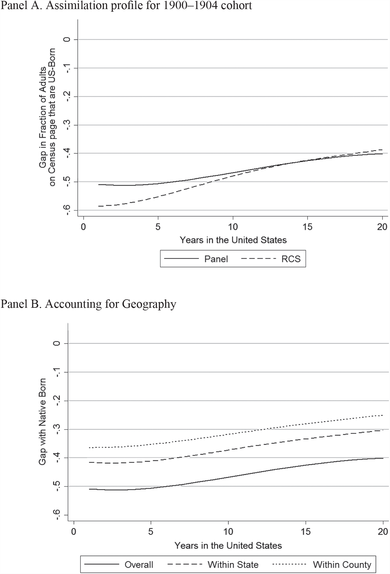
While the fall in immigrant segregation after 1910 suggests that immigrants spatially assimilated by quickly moving out of immigrant neighborhoods after arrival, this was not the case. Using linked census data from the 1910–1930 censuses, we show that the gap in having a U.S.-born neighbor between European arrivals and U.S.-born households closed slightly from 50 percentage points near arrival to 40 percentage points after 20 years of stay.Footnote 2 This result suggests that immigrants did spatially assimilate, but at a slow rate. A slow rate of spatial assimilation is consistent with a lack of convergence in occupational distributions for many source countries between 1900 and 1920 (Abramitzky, Boustan, and Eriksson Reference Abramitzky, Boustan and Eriksson2014); yet it contrasts with the quick rate of social assimilation after arrival in terms of English acquisition, immigrants adopting Anglicized names and immigrants giving their children Anglicized names (Abramitzky, Boustan, and Eriksson Reference Abramitzky, Boustan and Eriksson2016; Biavaschi, Giulietti, and Siddique Reference Biavaschi, Giulietti and Siddique2017; Ward Reference Ward2019). Therefore, despite the social assimilation of immigrants, the average neighborhood experience of immigrants was quite distinct from that of the native born.
We primarily focus on the segregation of immigrant households from native-born households, but there are alternative ways one could consider residential segregation. For example, one could measure how immigrant households were segregated from the third-plus generation households (in other words, U.S.-born to two U.S.-born parents), or how first and second-generation households (combined) were segregated from third-plus generation households. We create these additional measures when it is possible to separate second and third-plus generation households with parental birth place between the 1880–1930 censuses; however, since parental birthplace is not available for the entire period, our focus is on immigrant-native segregation. While we view different measures of segregation to be useful, our primary measure of immigrant-native segregation is important since immigrant segregation is associated with other key measures of assimilation, such as the acquisition of English fluency, intermarriage with native-born spouses and occupational attainment (e.g., Lieberson Reference Lieberson1963). Further, there is evidence that immigrant neighborhoods have long-run influences by shaping the educational and labor market outcomes of the second-generation (Aslund et al. Reference Aslund, Edin, Fredriksson and Gronqvist2011; Borjas Reference Borjas1995; Eriksson Reference Eriksson2018).
OVERVIEW OF HISTORICAL SEGREGATION MEASURES
One of the earliest studies to quantify immigrant segregation also demonstrates the key limitation of the literature. Lieberson (Reference Lieberson1963) measured immigrant segregation in ten major cities and showed that the dissimilarity index fell between 1910 and 1920, and also between 1930 and 1950. The dissimilarity index, one of the most used measures, quantifies how evenly a migrant population is distributed across sub-city geographical units (such as the city ward or enumeration district) (Massey and Denton Reference Massey and Denton1988).Footnote 3 However, one cannot reliably compare the 1910–1920 and 1930–1950 periods because the dissimilarity index uses the city ward as the sub-unit in the earlier period, but the census tract in the later period.Footnote 4 Besides the fact that city wards may be gerrymandered to reflect immigrant neighborhoods, they can also be more than 10 times larger than census tracts and therefore hide segregation; indeed, tract-level racial segregation measures yield dissimilarity scores about 15 points higher than ward-level measures (Cutler, Glaeser, and Vigdor Reference Cutler, Glaeser and Vigdor1999). Because of this switch from city wards to census tracts, Cutler, Glaeser, and Vigdor (Reference Cutler, Glaeser and Vigdor2008), who provide a long-run series of immigrant segregation between 1910 and 2000, show no absolute fall in dissimilarity between 1910 and 1940. This may lead a naïve reader to conclude that dissimilarity-based segregation did not fall in the early twentieth century if they do not note the change from ward-based to tract-based measures.Footnote 5 Cutler et al. (Reference Cutler, Glaeser and Vigdor1999) and Lieberson are careful to explain this measurement issue, but the decline of immigrant segregation in the early twentieth century has not yet been conclusively established.
The problem of using city wards to measure segregation is well known; therefore, some have resorted to census manuscripts to calculate segregation at finer levels of geography. However, this method is quite costly and therefore has been employed by only a few researchers (e.g., Thernstrom Reference Thernstrom1973; Kantrowitz Reference Kantrowitz1979; Zunz Reference Zunz1982).Footnote 6 The most comprehensive study using this method was the Philadelphia Social History Project, which plotted the addresses of more than 2.5 million Philadelphians between 1850 and 1880 (Hershberg Reference Hershberg1976).Footnote 7 After projecting 1930 census tract boundaries onto mid-nineteenth century maps, Hershberg et al. (Reference Hershberg, Burstein, Ericksen, Greenberg, Yancey and Hershberg1981) document that dissimilarity levels were low for Irish and German migrants in 1850 at about 0.30, but then then increased slightly to 0.35 in 1880. This small increase in dissimilarity-based segregation may be surprising given the large inflows of Irish and Germans after 1850; unfortunately, evidence on segregation for the years between 1850 and 1880 outside of Philadelphia is scarce.
This detailed evidence from Philadelphia has led to a consensus that segregation levels were lower in the earlier stages of the Age of Mass Migration and were higher for Southern and Eastern European sources. Yet Philadelphia may not be representative of the entire country. Recent efforts to digitize entire censuses allow researchers to look beyond Philadelphia; for example, Logan and Zhang (Reference Logan and Zhang2012) use the full-count 1880 census to estimate segregation measures for 67 cities across the country (Ruggles et al. Reference Ruggles, Genadek, Goeken, Grover and Sobek2018). They calculate segregation using enumeration districts, which are about the size of a census tract, a vast improvement over the city ward due to the enumeration district’s size and comparability with tract-based measures. They confirm that segregation levels were relatively low for immigrants from “old” sources in 1880 compared with those from “new” sources in the early twentieth century. However, Logan and Zhang also show that the variation in dissimilarity measures across cities was wide, which suggests that the selective city by city studies prior to 1880 may not be informative of the national average. While using enumeration districts to measure dissimilarity is promising, unfortunately enumeration districts did not exist prior to 1880, so one cannot use them to extend segregation measures back to 1850.
Even though measurement of segregation improves when researchers exploit census manuscripts, the literature has ignored segregation outside of larger cities. The literature’s focus on cities partially reflects that most immigrants settled there in the late nineteenth and early twentieth centuries, and that it is difficult to calculate a dissimilarity index in an area without city wards. However, about half of the migrant stock lived in rural areas throughout the nineteenth century, leaving a large gap in the literature. Rural settlement was especially common for Northern and Western Europeans in the Midwest, where many small towns today are still connected with an ethnic identity formed in the past, such as for the Dutch in Holland, Michigan and the Swiss in Berne, Indiana.
Our article continues the trend of using newly digitized census files to measure immigrant segregation. Since we observe everyone who is enumerated, we can exploit the census manuscripts to improve upon the major measurement issues in the literature. First, we cover more areas, including rural communities and smaller towns. Second, we measure segregation for decades and cities previously unquantified, particularly during the first major wave of immigration between 1850 and 1880 in cities outside of Philadelphia. Third, we provide measures that are comparable across time and space, and do not depend on inconsistently sized city wards. Finally, we measure segregation for non-European sources such as Mexico and China, which have been overlooked in the literature. All of this can be done due to the digitization of full-count census files between 1850 and 1940.
MEASURING IMMIGRANT ASSIMILATION BETWEEN 1850 AND 1940
We use full-count Census of Population data between 1850 and 1940 to measure immigrant segregation. These data are available from the University of Minnesota Population Center (Ruggles et al. Reference Ruggles, Genadek, Goeken, Grover and Sobek2018) and were accessed at the National Bureau of Economic Research (NBER).Footnote 8 We measure segregation based on the country of birth of the next-door neighbors’ household heads, which we can proxy because starting with 1850 the census was taken “on a line” such that households listed next to each other on a census page are reasonable proxies for next-door neighbors (Agresti Reference Agresti1980; Logan and Parman Reference Logan and Parman2017a). For example, the 1850 Census enumerator instructions directed census takers to keep houses “numbered in the order of visitation”; our assumption is that the order of households reflects close geographical proximity. Censuses prior to 1850, while also available from MPC, do not record country of birth; moreover, they were not enumerated on a line (Agresti Reference Agresti1980). We do not use the 1890 Census because most of the original manuscripts were lost in a fire.Footnote 9
We measure segregation of the foreign-born following Logan and Parman’s (Reference Logan and Parman2017a) method for black-white segregation with a one main modification: instead of using race for the in- and out-group, we use a specific country of birth for the in-group and the native born for the out-group.
There are several other ways one could create in-groups and out-groups. For example, between 1880 and 1930 we have further information on mother and father’s country of birth, so for these censuses we can alternatively define the out-group as U.S.-born to two U.S.-born parents. We could also define the out-group as all others from a different country of birth, not just the native born. We focus on using the native born as the out-group to be consistent with the immigrant segregation literature (e.g., Lieberson Reference Lieberson1963), and because living closer to natives may be related to linguistic assimilation or access to broader job networks. Here we will briefly describe the segregation measure, but those interested in more detailed information should reference Online Appendix B. While we focus on immigrant-native segregation, alternative measures such as immigrant segregation from any other country of birth are presented in Online Appendix C.
To create the neighbor-based segregation measure, we first keep the household head, dropping those in non-households and other non-heads in the household. This choice is a non-trivial restriction since many immigrants were also non-family members such as boarders or servants, and many also lived in non-household institutions such as employee camps. For example, about 90 percent of the migrant population lived in households between 1850 and 1940, leaving 10 percent in non-households.Footnote 10 Of those in households, about 10 percent were non-relatives of the head.Footnote 11 Moreover, by keeping the household head, we do not account for the birth place of the spouse. The segregation trends are mostly similar when one includes non-household heads and non-households in the measure (see Online Appendix C), but we will limit the measure to household heads for now to be consistent with Logan and Parman (Reference Logan and Parman2017a, Reference Logan and Parman2017b).
After keeping household heads and defining the nativity of the household based on the head, we then sort households by line number such that the households listed next to each other proxy for a next-door neighbor.Footnote 12 After sorting the census pages by line number, we create a variable which indicates whether either of the above or below household heads are native born, a variable on the extensive margin rather than the intensive margin of how many neighbors were native born. We only compare households to others on the same page rather than adjoining pages in case the next page was from a different neighborhood; however, the measure is largely unaffected if one includes those on the next or previous page in the measure.
It is key to note that the next-listed households proxy for the next-door neighbor, but do not always perfectly record the next-door neighbor. For example, the enumerator may have skipped a household if a respondent was not home or available for enumeration, only to return later. Also, there were no explicit directions for the enumeration order of apartment buildings. Nevertheless, treating those listed next to each other remains a reasonable proxy for close-by neighbor, as discussed by Agresti (Reference Agresti1980) and Logan and Parman (Reference Logan and Parman2017a). Moreover, Grigoryeva and Ruef (Reference Grigoryeva and Ruef2015) use geocoded data from 1880 Washington, DC, to verify that enumerators visited households in sequence along the street, finding that deviations from this sequence happened less than 5 percent of the time.
Given this proxy for next-door neighbors, for each county we know (1) the number of foreign-born households, (2) the number of native-born households, and (3) the number of foreign-born households with a native-born neighbor. The neighbor-based measure uses these values in the following formula:
 $${\eta _c} = {{E(\overline {nativ{e_c}} ) - nativ{e_c}} \over {E(\overline {nativ{e_c}} ) - E(\underline {nativ{e_c}} )}}$$
(1)
To calculate the segregation measure η c for country of birth c, the number of foreign-born households with at least one native-born neighbor (native c is compared with the expected number under the conditions of either random household location 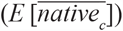 ${(E[\overline {nativ{e_c}} ])}$ or complete segregation from the native born
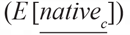 ${(E[\underline {nativ{e_c}} ])}$. Complete segregation from the native born suggests that the immigrant neighborhood (enumerated on a line) is surrounded by foreign-born households from other countries of birth. Therefore, complete segregation should lead to zero native-born neighbors
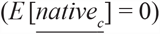 ${(E[\underline {nativ{e_c}} ] = 0)}$.Footnote 13
Given that the complete segregation suggests zero U.S.-born neighbors, Equation (1) can be rewritten as:
 $${\eta _c} = 1 - {{nativ{e_c}} \over {E(\overline {nativ{e_c}} )}}$$
(2)
This reformulation shows that the segregation measure is one minus the ratio of immigrant households with a native-born neighbor over the expected number under random assignment. For example, a segregation measure of 0.75 indicates that the actual number of immigrant households with a native-born neighbor is 25 percent of the expected number under random assignment. Likewise, a segregation measure of one (the maximum number) indicates that the actual number of native-born neighbors is 0 percent of the expected number.
The measure can be calculated for any level of geography, but in this article we present measures at the county- or city-level since we wish to describe the broad trends of segregation between 1850 and 1940. Note that the segregation measure can be noisy for counties or cities with a low number of immigrant households. However, aggregate numbers are weighted by population so this should not affect overall measures.
While the segregation measure typically ranges between zero and one, we document several important cases when the segregation measure goes below zero, especially for long-established sources. In fact, the minimum segregation level for a county and source country with more than 30 immigrant households is negative 1.25, which implies that there were 125 percent more immigrant households with a U.S.-born neighbor than expected under random assignment.Footnote 14 This would happen if immigrants from a given source were more likely to live next to U.S.-born households than next to immigrant households from other source countries. While negative segregation numbers are unusual in the literature, we find them to be informative about a source country’s interaction with both native and other source countries. Nevertheless, we provide an alternative measure in Online Appendix C that uses maximum integration with native-born households as the benchmark, rather than our preferred measure of random assignment of households. Under this alternative measure, the range of segregation is between zero and one.
Different segregation measures capture different forms of segregation (Massey and Denton Reference Massey and Denton1988); the neighbor-based measure is best understood as measuring the evenness of immigrant households in a county or city (Logan and Parman Reference Logan and Parman2017a). This interpretation is key for comparisons across time, place, and source countries. For example, if we measure that segregation is higher in country of birth, county, and year X relative to Y, then immigrant households were more unevenly distributed in X than in Y. Since the measure does not account for spatial distance or population density, it is possible that immigrants in a highly segregated urban county interacted with more U.S.-born individuals than immigrants in a less segregated rural county. Moreover, a highly segregated source country group may still interact with the native-born population if the source country has few immigrant households in the county.
Before showing trends in segregation, we can compare the results from the neighbor-based measure with other more common measures, such as the dissimilarity index or isolation index. The dissimilarity index measures the evenness of the immigrant population across sub-units in a city or county; the isolation index instead measures the exposure of an immigrant group to the U.S.-born population (Massey and Denton Reference Massey and Denton1988).Footnote 15 To calculate the dissimilarity and isolation indices, we use the enumeration district as the sub-unit when they are available between 1880 and 1940. After calculating all measures at the country of birth, county and decade-level and weighting by the number of immigrant households, the neighbor-based measure is positively correlated with the dissimilarity and isolation indices (0.69–0.70) (see Online Appendix Table A1). However, the correlation is much stronger in urban counties (0.74–0.77) than in rural counties (0.33–0.35). Since the correlation across measures is not perfect, it appears that the neighbor-based measure is capturing a different form of segregation, likely due to segregation within the enumeration district. Finally, recall that a benefit of the neighbor-based measure is that it can be extended backward to the beginning of the Age of Mass Migration in 1850, when enumeration districts are unavailable for calculating dissimilarity or isolation indices.
THE RESIDENTIAL SEGREGATION OF IMMIGRANTS BETWEEN 1850 AND 1940
The Broad Trends of Immigrant Segregation
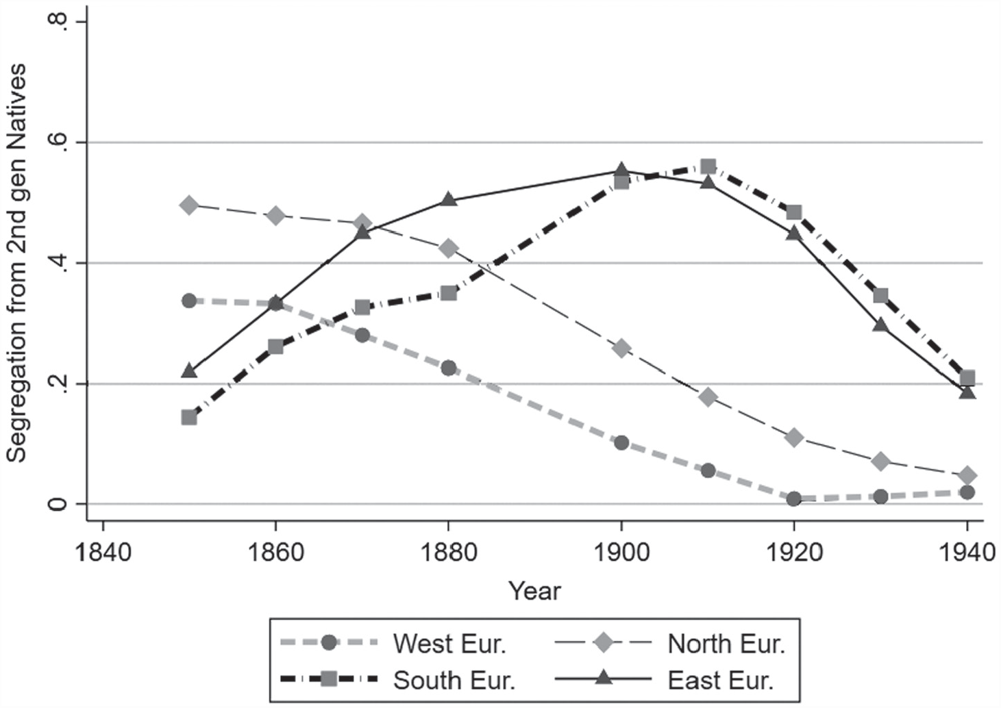
Figure 1 presents the trends of segregation levels from 1850 to 1940 after grouping countries of birth into either Western, Northern, Eastern, or Southern European.Footnote 16 The neighbor-based measure immediately confirms a few inferences in the literature, although here we show the national trend while the literature has been limited to urban areas. First, the segregation of Western Europeans during their peak immigration period in the mid-nineteenth century was less than that of Southern and Eastern Europeans during their peak period in the early twentieth century. Early Western Europeans (in other words, English, Irish, and Germans) started in 1850 with a segregation level of 0.34. On the other hand, Southern and Eastern European segregation levels were about 0.53–0.56 between 1900 and 1910. Therefore, the different immigrant waves had distinct experiences in the United States; this may reflect that Southern and Eastern Europeans entered a more highly urbanized country while earlier arrivals often moved to (less segregated) rural areas. We will explicitly measure differences in urban and rural segregation later.
NATIONAL SEGREGATION TRENDS BY SOURCE REGION, 1850 TO 1940

A second insight from Figure 1 is that Northern Europeans, a group often ignored in the literature due to their rural residences, were highly segregated in the mid-nineteenth century. We measure their level of segregation at 0.50 in 1850—slightly higher than Southern and Eastern European segregation in 1920. After their high levels of segregation in the mid-nineteenth century, Northern European segregation steadily decreased in the following decades, most rapidly after 1880. Interestingly, Northern European segregation decreased when inflows increased in the nineteenth century, which is the exact opposite relationship for inflows and segregation for Southern and Eastern Europeans in the late nineteenth and early twentieth centuries.
A third lesson from Figure 1 is that segregation trended downward for all source countries after 1910, indicating that immigrants became more integrated with the native-born population during the early twentieth century. This trend has long been suspected but never confirmed due to the switch from ward-based to tract-based measures in 1940; here, we are able to confirm it with a consistent measure between 1910 and 1940. Declining segregation after 1910 is likely because of the cutoff of immigration due to WWI and the immigration quotas.
Given the positive relationship between the number of foreign born and segregation across European source countries, we can test the relationship between these variables in a regression framework. To do so, we regress a source country’s segregation level on the source’s fraction households in the county. To account for numerous unobservables, we include the full set of county/year, country of birth/year, and county/country of birth fixed effects.Footnote 17 These fixed effects address, for example, changes in the county-specific economic conditions that may cause immigrants to cluster or disperse. After running the fixed effects regression, we find that a 1 percentage point increase in a source country’s percent in the county is associated with a 0.034-point increase in the segregation level, or 18 percent of mean level of segregation at 0.20 (see Online Appendix Table A2). However, the association is stronger for “new” sources (0.060-point increase) than for “old” sources (0.030), which may indicate that new arrivals from Southern and Eastern Europeans were more likely to cluster than those from Northern and Western Europe. Nevertheless, the regression evidence suggests that the rise and fall in segregation levels documented in Figure 1 partially reflects the rise and fall in inflows over time.
A common problem for immigrant segregation studies is that segregation measures decrease as immigrants’ native-born children age and live near the first generation; therefore, while immigrant-native segregation decreases, ethnic segregation (or living apart from those with a different ethnic background) may stay the same. This pattern may partially explain the strong downward trend in segregation during the twentieth century as source country groups became more established in the United States. To account for this possibility, we can measure immigrant segregation from the third-plus generation; that is, from households headed by someone who is U.S.-born to two U.S.-born parents. We can do this when information on mother and father’s country of birth is available between 1880 and 1930.
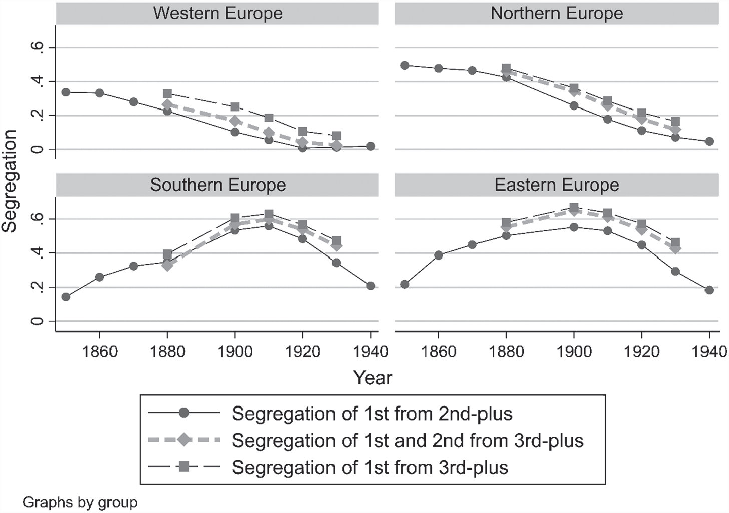
Immigrants were more segregated from the third-plus generation than from the second-plus generation, as seen in Figure 2. For instance, Western European segregation from the second-plus generation was effectively zero in 1920; however, from the third-plus generation, it was 0.11. This is likely because immigrant households were more integrated with second-generation households from their own ethnicity, perhaps because their children lived near their parents after forming their own households. The fall in segregation in the twentieth century was also slightly less rapid when one considers segregation from the third-plus generation. For example, the 21-point fall for Southern European from the second-plus generation (from 0.56 in 1910 to 0.35 in 1930) compares with a 16-point fall from the third-plus generation (0.63 to 0.47). However, the differences in trends across measures are not substantial, which suggests that the downward trend in segregation following 1910 is not primarily due to second-generation children living near their parents.
DIFFERENT WAYS OF MEASURING IMMIGRANT SEGREGATION

Given the discrepancies between segregation from the second-plus generation and segregation from the third-plus generation, note that we primarily present measures of immigrant segregation and not ethnic segregation. One possible way to measure ethnic segregation is to combine the first and second generations together as a proxy for an ethnic group, and then measure their segregation from third-plus generation households. We show these measures of “ethnic” segregation in Figure 2 for different regions of Europe, benchmarking them against segregation of the first from second-plus generation and segregation of the first from third-plus generation. Figure 2 shows that segregation of the first and second-generations from the third-plus generation is less than segregation of the first from the third-plus generation, which is reasonable if there is spatial assimilation across generations. We would prefer to measure segregation from the third-plus generation throughout the 1850–1940 period, but it is only available when information on mother and father’s county of birth is included between 1880 and 1930.
Yet combining the first and second generations to measure ethnic segregation is still somewhat unsatisfactory since third-generation households may descend from the same countries of birth as their first and second-generation neighbors. At some point it is unclear which generation no longer has attachment to ethnicity, partially because intermarriage was more common for higher-order generations (Alba Reference Alba1985; Wildsmith, Gutmann, and Gratton Reference Wildsmith, Gutmann and Gratton2003). This problem does not hold for racial segregation, where race was strongly transmitted to an individual’s children, grandchildren, and great-grandchildren during this period. Given the complexities of measuring ethnic segregation, our main results are for immigrant-native residential segregation. Nevertheless, note that the various ways of measuring segregation in Figure 2 produce roughly the same trends of segregation, albeit different levels.
Measures by Source Country
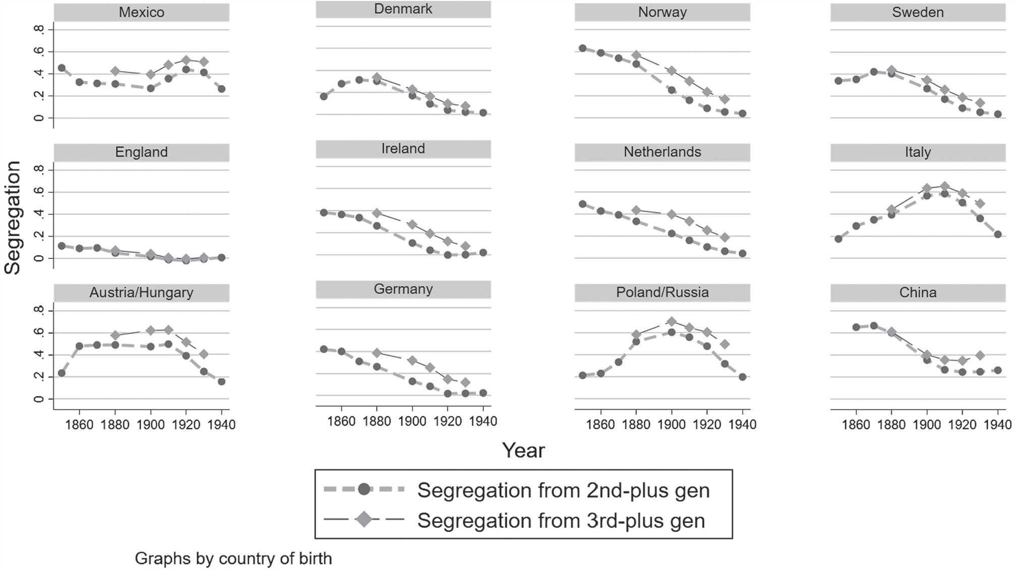
We split the broad regions of Western, Northern, Eastern, or Southern European into 12 selected countries of birth in Figure 3 (see Online Appendix Tables A3 and A4 for underlying estimates for all countries).Footnote 18 This figure reveals starker differences across source countries than for the aggregated regions of Northern, Western, Southern, and Eastern Europe. For example, English immigrants were the least segregated of all sources and remained at a low level of segregation throughout the entire period. In fact, English immigrants were perfectly integrated with native-born households in some decades, perhaps because most native born were descendants of England during the mid-nineteenth century. Standing out on the opposite end of the segregation spectrum was Norway, which was much more segregated than its Northern European counterparts of Denmark or Sweden.
IMMIGRANTS WERE MORE SEGREGATED FROM NATIVE-BORN WITH NATIVE-BORN PARENTS

Mexican and Chinese immigrants were highly segregated, but not much more so than Italians or Russians/Poles during their peak of immigration between 1900 and 1910. The peak of segregation for Mexicans was at 0.44 in 1920, the first decade immediately following the Mexican Revolution when hundreds of thousands fled the country for safety; yet many economic migrants came at the same time and worked in segregated mining towns and farming areas. Mexican segregation, like European segregation, fell following the 1920s, perhaps reflecting the mass movement back to Mexico due to the Great Depression and deportations. On the other hand, the peak of Chinese segregation was earlier in 1870 at 0.67 when there were relatively few Chinese household heads (~11,000). The segregation of Chinese fell in the next few decades to a low of 0.24 in 1920, lower than the level for Southern and Eastern Europeans. Therefore, the Chinese were indeed highly segregated, but primarily in the nineteenth century.
Measuring Segregation across Urban and Rural Areas
In this section, we turn to document something that has been commonly ignored in the literature: segregation in rural areas. We are primarily interested in how the level of segregation differed across rural and urban areas, which will uncover whether the literature’s focus on urban areas has provided an incomplete guide to the history of immigrant segregation. We can further examine the trend in segregation levels across urban and rural areas, which may indicate whether urban phenomenon, such as the rise of mass transit or urban factories, led to increased segregation between 1850 and 1940. If segregation trended similarly in rural and urban areas, then this suggests that cultural or demographic factors were more influential, such as a preference for living in an ethnic community.
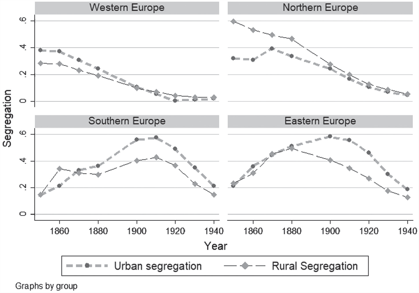
Figure 4 plots segregation by rural and urban counties for the four European source regions (Eastern, Northern, Southern, and Western) between 1850 and 1940.Footnote 19 Following Logan and Parman (Reference Logan and Parman2017a), we define counties to be urban if more than 25 percent of the population lived in an IPUMS-defined urban area, which are cities or incorporated areas with more than 2,500 residents. The figure illustrates two key points. First, while urban segregation was often higher than rural segregation, Northern European rural segregation was higher than urban segregation in the nineteenth century. This was especially true between 1850 and 1880 when rural Norwegians, Swedes, and the Dutch were more segregated than their urban counterparts. Rural segregation could be quite high. For instance, Dutch rural segregation in 1850 was higher than Irish urban segregation at the same time, which may be surprising since this included the infamous Irish slums in Boston and New York during the Great Famine (Anbinder Reference Anbinder2001; Handlin Reference Handlin1959). Moreover, Dutch rural segregation in the mid-nineteenth century was near that of Southern and Eastern European urban segregation between 1900 and 1910. Overall, rural Northern Europeans in the nineteenth century were highly segregated.
RURAL SEGREGATION WAS OFTEN HIGHER THAN URBAN SEGREGATION IN THE NINETEENTH CENTURY

While rural counties were more segregated than urban counties for nineteenth century Northern Europeans, this pattern did not hold for other source regions, especially after 1880 when the inflows of “new” source immigrants from Southern and Eastern Europe increased rapidly. Despite often hailing from rural communities, Southern and Eastern Europeans overwhelmingly located in urban areas after arrival (more than 90 percent in 1910). One consequence of this large urban inflow appears to be that urban segregation increased disproportionately relative to rural segregation after 1880 (see Figure 4). For example, while rural and urban segregation for Eastern Europeans was similar at 0.50 in 1880, it diverged by 1900 when urban segregation had increased to 0.58 and rural segregation decreased to 0.41.
It could also be that urban segregation increased more than rural segregation because inflows had a stronger effect on segregation in urban counties than in rural counties. However, this does not appear to be true. If one splits the sample by rural and urban counties and estimates the association between the county’s fraction foreign born and segregation in a fixed effects regression (see Online Appendix Table A2), then the association is similar in size across rural and urban counties. Specifically, a 1 percentage-point increase in foreign-born households is associated with a 0.033 increase in rural segregation and 0.036 increase in urban segregation.
Besides higher inflows, the relative increase of Southern and Eastern European urban segregation between 1880 and 1910 could also be due to urban-specific factors such as expansion of public transportation that could allow immigrants to sort more easily into neighborhoods further from work. There was also an increase of large-scale manufacturing plants, many of which relied on migrant labor and could cause immigrant enclaves to form close by. These urban-specific factors could also impact Western and Northern European segregation, but the aggregate trends in Figure 3 do not show a relative increase of urban over rural segregation for these “old” sources. Rather, Western and Northern European urban and rural segregation converged throughout the twentieth century. Of course, urban-specific forces may have affected Western and Northern European residential patterns in ways that are hidden in the aggregate fall of segregation. Ultimately, more research is needed to explore what influenced rural and urban segregation patterns throughout this period.
The Most Segregated Areas in America, 1850–1940
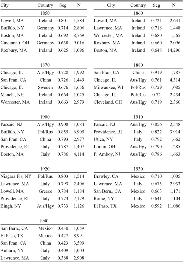
Urban phenomena clearly did play a role in residential patterns since some of the most highly segregated towns in our data were factory towns. Table 1 lists the cities with the highest segregation levels by year for sources that had more than 1,000 household heads in town—thus, the list includes both major and minor cities. The most highly segregated cities across the entire 1850 to 1940 period were not the major entry points of New York and Boston, but rather textiles towns; for example, the Irish in 1850 Lowell and Lawrence, Massachusetts were highly segregated. One of the most segregated sources and cities in the entire data is Austro-Hungarians in 1900 Passaic, New Jersey (0.908). Other highly segregated manufacturing towns were Bridgeport, Connecticut, and Buffalo, New York. Yet manufacturing hubs do not completely dominate the list of most segregated source countries and towns. Chinese immigrants in 1880 San Francisco were also highly segregated—the highest level of segregation of all cities and years in Table 1 (0.919). A high level of Chinese segregation may reflect the discriminatory factors that led to the 1882 Exclusion Act (Carter Reference Carter2012).
TOP SEGREGATED SOURCE COUNTRIES AND CITIES WITH MORE THAN 1,000 HOUSEHOLDS

Notes: The table lists the city, country of birth, segregation level, and number of household heads for each source country. Segregation is measured from native-born households.
Sources: 1850 to 1940 full-count United States Censuses (Ruggles et al. Reference Ruggles, Genadek, Goeken, Grover and Sobek2018).
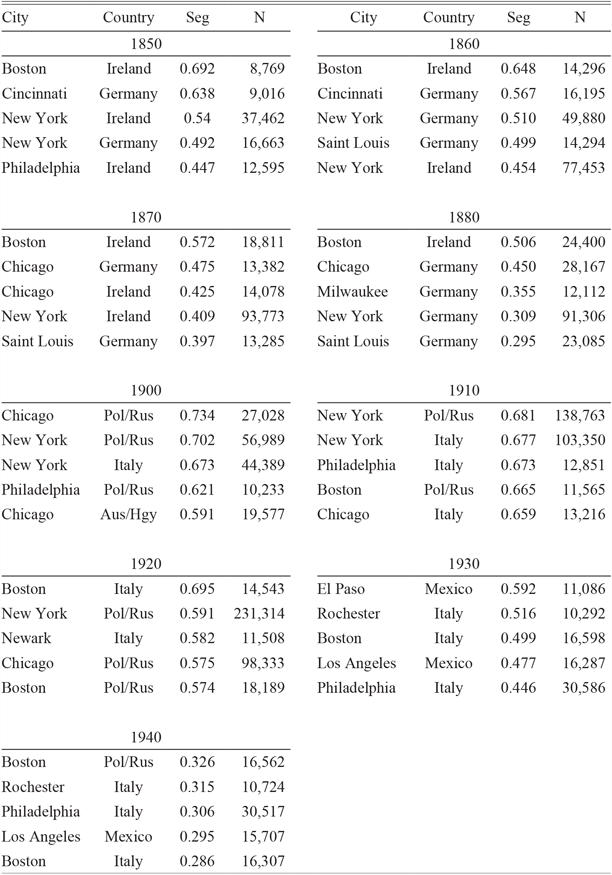
The major entry ports are largely absent from the list of the most segregated cities in Table 1. This may be surprising since new arrivals were often the most segregated. To look at the segregation level of larger cities, which has been the dominant interest of the literature, we limit the sample to cities with a sizeable immigrant population in Table 2.Footnote 20 Based on this list of large cities, Irish immigrants in Boston were the most highly segregated source between 1850 and 1880, reflecting those fleeing the Great Famine and its aftermath. Yet even the Irish in mid-nineteenth century Boston were not as highly segregated as Irish immigrants in the small factory towns outside of Boston, as we saw from Table 1. For example, the level of segregation for the Irish in 1850 Boston was 0.692, while it was 0.801 in Lowell in the same year. At the opposite end, English immigrants in New York City had a negative level of segregation in 1860, indicating that they were more likely to live next to a U.S.-born household than next to a foreign-born household from Germany or Ireland.
TOP SEGREGATED SOURCE COUNTRIES AND CITIES WITH A LARGE POPULATION

Notes: The table lists the city, country of birth, segregation level and number of household heads for each source country. Results only shown for cities with more than 10,000 households from a given source, except for 1850 when the limit is 8,000. Segregation is from native-born households.
Sources: 1850 to 1940 full-count United States Censuses (Ruggles et al. Reference Ruggles, Genadek, Goeken, Grover and Sobek2018).
Some of the highest segregation levels in large cities between 1850 and 1940 were for “new” source immigrants in the early twentieth century rather than “old” sources during the nineteenth century. This is consistent with evidence from Philadelphia in the nineteenth and twentieth centuries, but our data broaden the result to other cities (Hershberg et al. Reference Hershberg, Burstein, Ericksen, Greenberg, Yancey and Hershberg1981). The high levels of segregation did not persist long into the twentieth century; after the immigration quotas were enacted in the 1920s, New York City fell almost entirely off the list of most segregated cities. Instead of the major Northeastern and Midwestern cities, Mexicans in El Paso topped the list in 1930, reflecting the changing composition of arrivals due to the quotas. Besides these entry points of New York and El Paso, several large cities in the Midwest were highly segregated, such as Germans in Cincinnati, Saint Louis, and Chicago, and immigrants from Poland/Russia in 1900 Chicago.
The most highly segregated urban areas were smaller towns associated with manufacturing, but how did segregation in these factory towns compare to segregation in rural areas? Table 3 lists the most segregated rural counties between 1850 and 1940. Well known ethnic rural communities appear on this list, such as the Dutch in 1860 Ottawa County, Michigan, where the town of Holland is located. Norwegian farming communities in Minnesota and Wisconsin also top the list during Norway’s high inflow periods between 1860 and 1880. In fact, Norwegians in Otter Trail County, Minnesota were the most highly segregated source country in a rural county at 0.722, more segregated from native-born households than the 1850 Irish in Boston.
TOP SEGREGATED SOURCE COUNTRIES AND RURAL COUNTIES WITH MORE THAN 1,000 HOUSEHOLDS

Notes: The table lists the county, country of birth, segregation level and number of household heads for each source country. This is based on counties that have at most 25 percent of the population in an urban area (>2,500 residents).
Sources: 1850 to 1940 full-count United States Censuses (Ruggles et al. Reference Ruggles, Genadek, Goeken, Grover and Sobek2018).
Not all highly segregated rural counties were associated with farming; in fact, by the turn of the twentieth century, the most segregated rural counties were in areas associated with coal mining and steel production in Western Pennsylvania. These counties topped the list between 1900 and 1940, including Somerset, Indiana (PA), Fayette, and Westmoreland County. Segregation in these rural counties was so high that it rivalled that of New York and Boston. Besides these mining areas in the Northeast, mining and agriculture in the American Southwest also led to high segregation levels for Mexicans in New Mexico and California.
Comparison to Black-White Segregation
Segregation levels for immigrants were high for some countries, but how did these levels and trends compare to those of black-white segregation? This is a common question in the literature, dating back to early work from Lieberson (Reference Lieberson1963, Reference Lieberson1980); thus, it is worth quickly reviewing results from dissimilarity and isolation measures already in the literature. First, black-white segregation was about equal to Southern and Eastern European segregation in 1910 (Cutler, Glaeser, and Vigdor Reference Cutler, Glaeser and Vigdor1999, Reference Cutler, Glaeser and Vigdor2008). Following 1910, black-white segregation and immigrant segregation diverged such that black-white segregation increased and Southern and Eastern European segregation decreased. However, these comparisons come from select cities and miss the large set of African Americans and foreign born who lived in rural areas. Given that we follow Logan and Parman’s (Reference Logan and Parman2017a) methodology to measure segregation, it is straightforward to compare our estimates of immigrant segregation to their estimates of black-white segregation from 1880 to 1940.
Before comparing black-white to immigrant segregation, recall the key caveat that black-white segregation differs from immigrant-native segregation because racial status transmits across generations while immigration status does not. Nevertheless, we continue with this comparison given the interest in the literature. In addition to comparing black-white segregation to immigrant-native segregation, we also compare it to the segregation of the first and second generation from the third-plus generation, which is a proxy for ethnic segregation.
The neighbor-based measure confirms the prior literature in that immigrant-native and black-white segregation started out at similar levels in 1910 but diverged afterwards. Logan and Parman (Reference Logan and Parman2017b) measure black-white segregation at about 0.58 in 1910, which is similar to our measures of immigrant-native segregation for Southern Europeans (0.56) and Eastern Europeans (0.54). However, if one measures segregation as the first and second generation from the third-plus generation instead of the first from the second-plus generation, then segregation for Southern and Eastern Europeans (0.60–0.61) was slightly higher than black-white segregation in 1910. Of course, these national levels mask significant variation by city and source country where black-white segregation was higher than ethnic segregation, as pointed out by Lieberson (Reference Lieberson1980).
From this roughly equal level of immigrant and black-white segregation in 1910, the neighbor-based measure shows that black-white segregation increased, while immigrant segregation decreased. In 1940, Logan and Parman (Reference Logan and Parman2017b) calculate black-white segregation at 0.67, which was much higher than Southern and Eastern European immigrant-native segregation at 0.18–0.21. Segregation of the first and second generation combined also trended downward after 1910, suggesting that black-white segregation was also less than “ethnic” segregation in 1940. Segregation levels for Asians and Mexicans were also lower than for African Americans in 1940, suggesting that African Americans were unique among racial and immigrant sources for their high levels of segregation in the middle of the twentieth century.
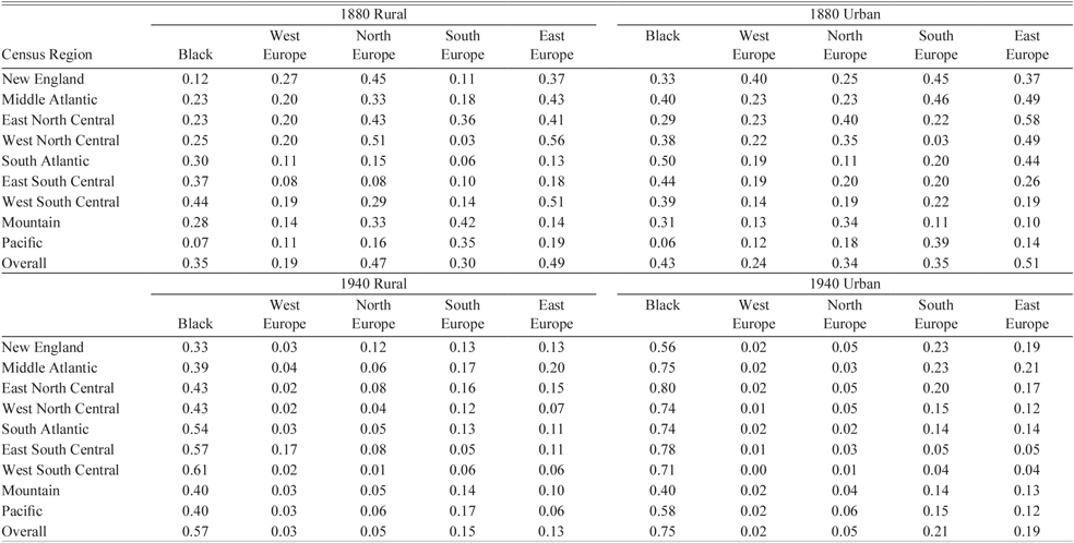
The difference between black-white and immigrant-native segregation at the national level may mask rural and urban differences since most of the black population was rural while most immigrants were urban. Further, African Americans primarily lived in the South, while immigrants lived in the Northeast and Midwest. If one limits the sample to the southern census regions, then 1880 black-white segregation was higher than immigrant-native segregation in both rural and urban areas (see Table 4). Therefore, the few immigrants who did move south were not more segregated than their southern black or non-southern immigrant counterparts. On the other hand, black-white segregation in the North and Midwest census divisions was not especially high; for example, black-white rural segregation was lower than Northern European rural segregation, and black-white urban segregation was lower than Eastern European urban segregation. However, by 1940, black-white segregation was much higher than immigrant-native segregation across all census regions and rural/urban counties.
SEGREGATION BY CENSUS REGION AND RURAL OR URBAN COUNTIES, COMPARISON TO LOGAN AND PARMAN (2017)

Notes: The results show immigrant-native segregation, or segregation of the first from second-plus generation. Black-white segregation levels taken from Logan and Parman (Reference Logan and Parman2017, Table 3). Means are weighted by the number of immigrant households in county (or number of black households for black-white segregation). Urban is defined as those with more than 25 percent of the population in an urban area. Counties that were rural in 1880 may be urban by 1940.
Sources: 1880 and 1940 full-count United States Censuses (Ruggles et al. Reference Ruggles, Genadek, Goeken, Grover and Sobek2018).
Robustness of Segregation Trends
In the Online Appendix, we gauge the robustness of these segregation patterns to alternative measures. One potential issue with the segregation measure is that it is based on household heads, which therefore misses non-household heads or those in non-households. This is nontrivial since many immigrants lived as boarders in houses or in mining or railroad camps, or had native-born spouses. In Online Appendix C, we present alternate national trends based on the proportion of adult native-born on a census page, which includes all individuals older than 18, rather than just household heads. The resulting estimates from this “page-based” measure have a correlation across counties and all years of 0.941 with the main household-based measure. Therefore, the results from the page-based method are consistent with most results from the neighbor-based measure; for example, the relative levels and trends by country of birth are similar, as well as the levels and trends across rural and urban areas.
Another approach one could take is to change the out-group from the native born to those from any other country of birth. Our approach of measuring segregation from the native born is like that of Lieberson (Reference Lieberson1963); however, an immigrant population highly segregated from natives may be more integrated with immigrants from other sources. In Online Appendix D, we present results on segregation from any other country of birth, which show mostly the same trends as our preferred measure: the county, year, and source level correlation between segregation from the native-born and segregation from all other countries is 0.837. However, Eastern European segregation does depend on the out-group since they were highly segregated from the native-born, but relatively integrated with immigrants from other countries. It is possible that there were stages of spatial assimilation for some sources where one first lived near fellow countrymen, then near immigrants from other sources, and then near the native born. It is also possible that for Eastern Europeans, segregation by country of birth is a poor measure of ethnic group since country of birth does not coincide well with linguistic group.
THE SPATIAL ASSIMILATION OF IMMIGRANTS
The evidence so far shows that segregation tended to rise and fall with inflows during the twentieth century, especially following WWI and the immigration quotas. This suggests that immigrants were highly segregated soon after arrival, but then eventually moved out of the enclave as they became more socially assimilated; however, it could also be that those who were highly segregated returned home and therefore the overall segregation level fell. This may be especially important in the early twentieth century when the return flow is estimated to be above 40 percent of the inflow (Bandiera, Rasul, and Viarengo Reference Bandiera, Rasul and Viarengo2013; Gould Reference Gould1980). In this section, we estimate the rate at which immigrants moved closer to the native born with individual-level data that follow 1900–1919 arrivals for up to 20 years after arrival.Footnote 21 The individual-level data are advantageous since we can simply use the indicator variable for whether an above- or below-listed household head is native born, rather than the aggregated measure at the county level. Thus, we can capture spatial assimilation due to movements within the county, which is key to the Park and Burgess (Reference Park and Burgess1925) model of spatial assimilation due to movement from the center to the outer rings of the city. We also use the fraction of adults on the page that are native born, which has the advantage of including both non-household heads and non-relatives in the segregation measure.Footnote 22 Both measures lead to the same qualitative results.
The longitudinal data take the population of 18- to 40-year-old European-born males in the 1910 and 1920 censuses who arrived in the previous ten years, and then track them ten years later to the next census.Footnote 23 The data were created based on machine-learning techniques from Feigenbaum (Reference Feigenbaum2016) and were first presented in detail in Ward (Reference Ward2019). The linking process accounts for possible Americanization of first name by linking on the Americanized version of the immigrant’s first name.Footnote 24 Given that linking tends to produce non-random samples, the sample is weighted to be representative on observables according to the census (Bailey et al. Reference Bailey, Cole, Henderson and Massey2017). The final data include 103,392 male immigrants linked from 1910–1920, and 113,799 linked from 1920–1930.
To estimate the rate of spatial assimilation, or the rate at which immigrants converged to natives in the likelihood of having native-born neighbors, we pool the immigrant panel with a 1 percent random sample of natives from the 1910 to 1930 censuses and from the same birth cohorts. The sample of U.S.-born consists of second-plus generation males (both black and white) who lived in the entire country; while our main comparison is at the national level, we will later limit the comparison to be within state or within county.
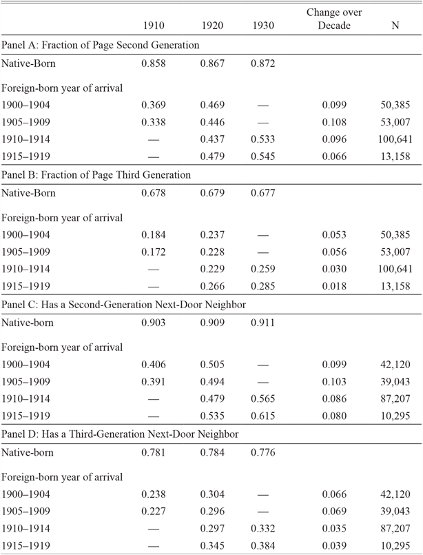
Table 5 splits the 1900–1919 arrivals in the panel data into five-year cohorts and shows that recent arrivals were highly segregated soon after arrival from the native-born population. For example, with 1905–1909 arrivals, only 34 percent of adults on the same page were native-born in 1910.Footnote 25 After starting at this low point, immigrants were more likely to live near native-born neighbors by the next decade; for 1905–1909 arrivals, the fraction native-born neighbors increased from 34 to 45 percent. Importantly, since we have a panel, this increase over time is not driven by the selective return of those with fewer native-born neighbors.
SPATIAL ASSIMILATION USING LONGITUDINAL DATA

Notes: Data are also from a 1910, 1920, 1930 1 percent random sample of natives. The sample sizes for the native born in Panels A and B are 181,464 in 1910, 210,324 in 1920, and 253,841 in 1930. Next-door neighbor is proxied with an indicator variable that is equal to one if the above- or below-listed household head on the census manuscript is native born. The sample sizes for the native born in Panels C and D are 97,980, 118,238, and 146,079.
Sources: Linked samples between the 1910–1920 census and 1920–1930 census (Ward Reference Ward2019) pooled with 1 percent random sample from 1910, 1920, and 1930 Censuses (Ruggles et al. Reference Ruggles, Genadek, Goeken, Grover and Sobek2018.)
While immigrants were more likely to live near native-born individuals in the decades after arrival, they were still much less likely to have a native-born neighbor than the average native-born male. Since more than 90 percent of native-born males had a native-born neighbor, about double the number for immigrants, the gap between immigrants and natives in the fraction native-born on the census page was large. The gap between natives and immigrants decreased from 50 to 41 percentage points for the 1905–1909 cohort between the 1910 and 1920 censuses, or by about 20 percent.
A natural question is whether the increase in native-born neighbors is due to sorting into areas with more native-born individuals or because the neighborhood around the household changed. To estimate this, we split the sample into those who remained in the same neighborhood and those who changed neighborhoods; we define one to be in the same neighborhood if his enumeration district in the first census overlaps with his enumeration district in the second census. Unfortunately, this approach can only be implemented for cities with digitized enumeration district maps, which we have for ten Northern cities or 27 percent of our sample (Shertzer, Walsh, and Logan Reference Shertzer, Walsh and Logan2016).Footnote 26 We can therefore estimate how the fraction native-born on page changes for those who remained in the same enumeration district compared with those who changed districts.
This enumeration-district analysis suggests that spatial assimilation was primarily due to immigrants moving into different enumeration districts rather than the composition of the district changing over time. For example, the fraction U.S.-born on the census page increased from 34 to 39 percent for those who remained in the same enumeration district (see Online Appendix Tables A8 and A9). On the other hand, for those who moved districts (either within the same city or outside the city), the proportion of U.S.-born increased from 32 to 46 percent, or nearly three times the increase of those who remained in the same district. Moreover, changing districts was incredibly common in our linked sample: only 9.3 percent of immigrants lived in the same one 10 years later. When one combines these facts, district switchers contributed 96.6 percent of the growth in fraction U.S.-born neighbors, while district stayers contributed 3.4 percent.
We can further pool the panel data with repeated cross sections of foreign household heads or individuals to gauge selection into return migration.Footnote 27 Since the panel contains only permanent migrants and the cross sections contain both permanent and temporary migrants, the difference between the panel and cross sections recovers characteristics of temporary migrants (Abramitzky, Boustan, and Eriksson Reference Abramitzky, Boustan and Eriksson2014). Figure 4 plots the assimilation profile for both the panel and for a repeated cross section using a standard assimilation specification in the literature and shows a slow convergence in the fraction of the page that are U.S.-born.Footnote 28
Based on the comparison of the panel and cross-sectional data, return migrants were less likely to have a native-born neighbor since the cross section estimates a larger gap at arrival than the panel (58.4 versus 50.1 percentage points). One concern with this interpretation is that the difference between panel and repeated cross sections is not due to selection into return migration but because we are more likely to link those in less segregated areas than in highly segregated areas. Moreover, this difference is not fully accounted for by weighting on observable characteristics. While this may be possible, there is also evidence against this point since those in highly segregated areas were less likely to Americanize their names; this suggests that we may be more likely to link those in highly segregated areas since they were less likely to change names across censuses in ways not captured by the Americanization algorithm (Carneiro, Lee, and Reis Reference Carneiro, Lee and Reis2015). Either way, return migrants having fewer native-born neighbors is consistent with direct evidence that return migrants were negatively selected on occupational income (Ward Reference Ward2017). The result that return migrants had fewer native-born neighbors holds for all 1900–1919 cohorts, which can be seen in the cohort effects plotted in Online Appendix Figure A3.
The assimilation profile compares the average immigrant to the average native born, so the wide immigrant-native gap in native-born neighbors partially reflects that natives and immigrants lived in different regions of the country. We can narrow the comparison to be within state or within county, which we show in Panel B of Figure 5. The within-county gap in fraction U.S.-born on a page is smaller than the national gap: for instance, the estimated national arrival gap is –0.50 for the 1905–1909 cohort, but it is –0.36 within county. Yet the rate of spatial assimilation does not change when controlling for county of residence, so the immigrant-native gap in U.S.-born on the census page still narrowed at a slow rate within county.
SPATIAL ASSIMILATION IN THE DECADES AFTER ARRIVAL

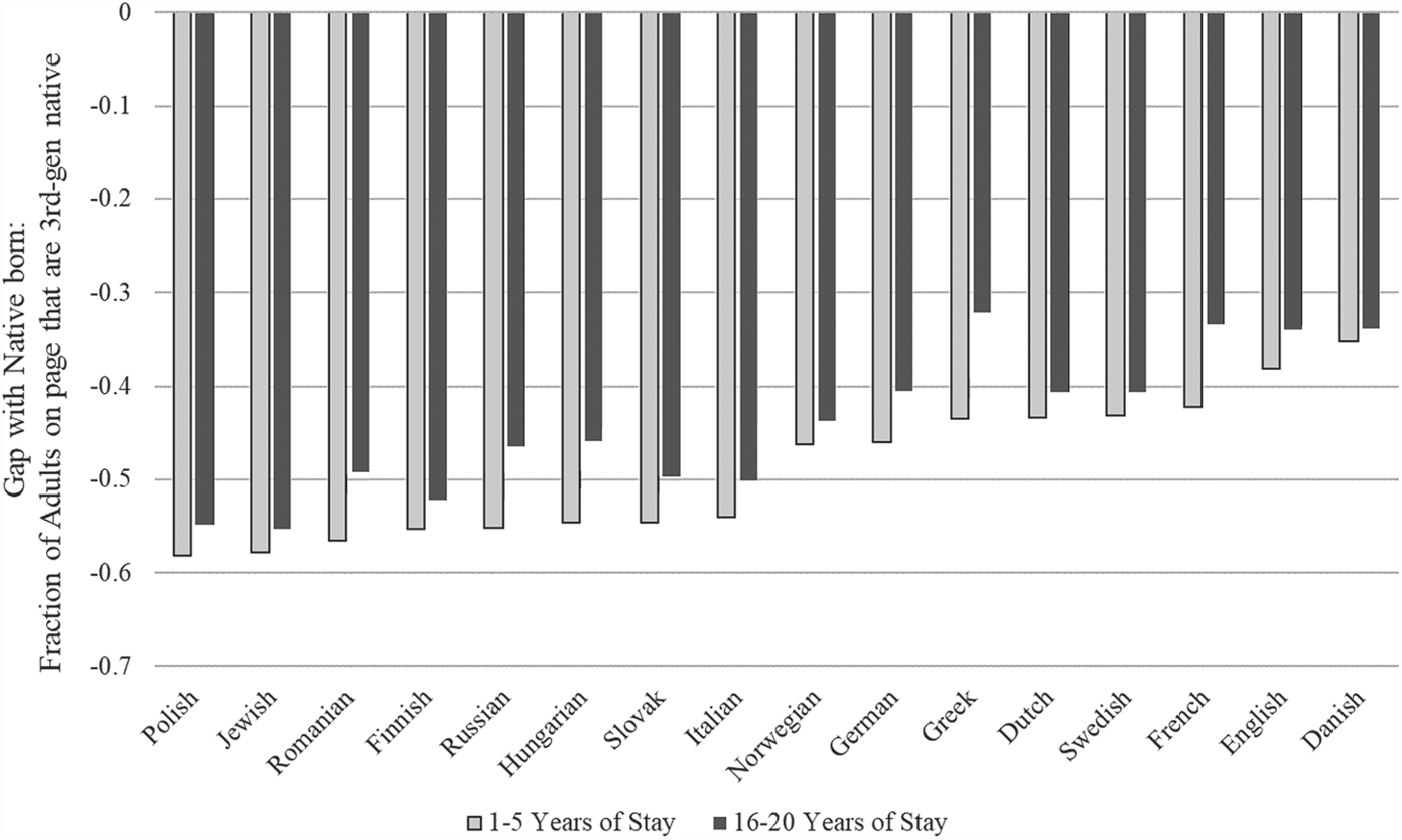
While immigrants on average arrived highly segregated from natives and did not converge at a quick rate, this masks heterogeneity by source country in Figure 6. Consistent with the county-level segregation measure, the individual-level panel data show that Southern and Eastern Europeans arrived the most highly segregated, while those from Northern Europeans and England arrived less segregated. While the size of the initial gaps varied across source countries, the convergence of gaps was similar across sources such that there was little to no closure after 16 to 20 years of stay. Overall, the evidence from the panel data confirms that immigrants’ experience in the United States during the early twentieth century was distinct from that of natives, despite immigrants having a similar level of occupational status and assimilating quickly in terms of English proficiency, intermarriage, and Anglicization of names (Abramitzky, Boustan, and Eriksson Reference Abramitzky, Boustan and Eriksson2014, Reference Abramitzky, Boustan and Eriksson2016; Biavaschi, Giulietti, and Siddique Reference Biavaschi, Giulietti and Siddique2017; Ward Reference Ward2019).
SPATIAL ASSIMILATION BY SOURCE COUNTRY BETWEEN 1910 AND 1920

CONCLUSIONS
In this article, we present the first measures of immigrant residential segregation that are consistent across time and space during the Age of Mass Migration and beyond (1850 to 1940). Our measure adapts the method first introduced by Logan and Parman (Reference Logan and Parman2017a) to immigrants, where we proxy for the next-door neighbor based on the ordering of the census enumeration sheet. We provide new estimates of immigration segregation that are consistent across time and space, and cover countries of birth and areas of the country where segregation was previously unquantified.
The new measures revise our understanding of immigrant residential segregation in American history. First, we show that segregation was sometimes high in areas previously unmeasured, especially in small factory towns and nineteenth century rural communities. Therefore, immigrant segregation was not purely an urban phenomenon, despite the sole focus on urban areas in the literature. Second, we show that segregation was high for non-European sources, such as for Chinese and Mexican immigrants; while Chinese segregation was uniquely high in the nineteenth century, both Mexican and Chinese segregation were similar in magnitude to European segregation in the twentieth century. While the neighbor-based measure broadens our knowledge on segregation by covering more areas, sources and time periods, it does not overturn prior results from city ward/census tract-based studies, such as the decrease in segregation during the early twentieth century and that “new” sources tended to more segregated during the early twentieth century than “old” sources in the nineteenth century (Cutler, Glaeser, and Vigdor Reference Cutler, Glaeser and Vigdor2008; Hershberg et al. Reference Hershberg, Burstein, Ericksen, Greenberg, Yancey and Hershberg1981; Lieberson Reference Lieberson1963).
Our primary aim is to present a measure of the broad segregation patterns between 1850 and 1940. By limiting ourselves to a birds-eye view of segregation, we do not explore the rich detail for specific sources, cities, counties, or time periods. For instance, there is little knowledge about the causes and consequences of segregation during the high immigration period prior to the Civil War, when German and Irish immigrants arrived after fleeing famine and political violence. More research could be done on the effects of segregation; for example, one could estimate how social and economic assimilation depended upon on arriving in a highly segregated neighborhood, or the effect of segregation on subsequent generations’ outcomes.Footnote 29 One could also relate the measure to the public economics literature, for example, by exploring how public good provision was related to ethnic segregation. Given the extensive detail in the newly digitized census manuscripts, there is much to explore.