1. INTRODUCTION
An artificial neural network (ANN) is inspired by the manner of biological nervous system, such as human brain to process the data, and is one of the numerous algorithms used in machine learning and data mining (Dasarthy, Reference Dasarthy1990; Kemp et al., Reference Kemp, MacAulay, Garner and Palcic1997; Goebel & Gruenwald, Reference Goebel and Gruenwald1999; Hegland, Reference Hegland2003; Kantardzic, Reference Kantardzic2011). In a feedforward neural network (FFNN), data processing has only one forward direction from the input layer to the output layer without any backward loop or feedback connection (Bose & Liang, Reference Bose and Liang1996; McCloskey, Reference McCloskey2000; Andonie & Kovalerchuk, Reference Andonie and Kovalerchuk2007; Kantardzic, Reference Kantardzic2011). Learning is an imperative property of the neural network. There are many types of learning rules used in the neural networks, which fall under the broad categories of supervised learning, unsupervised learning, and reinforcement learning. Most approaches to unsupervised learning in machine learning are statistical modeling, compression, filtering, blind source separation, and clustering (Hegland, Reference Hegland2003; Han & Kamber, Reference Han and Kamber2006; Andonie & Kovalerchuk, Reference Andonie and Kovalerchuk2007; Kantardzic, Reference Kantardzic2011). In this study, the clustering aspect of unsupervised neural network learning is considered. Learning from observations with unlabeled data in an unsupervised neural network clustering is more desirable and affordable than learning by examples in supervised neural network classification because preparing the training set is costly, time consuming, and possibly dangerous in some environments. However, to evaluate the performance of unsupervised learning, there is no error or reward indication (Kohonen, Reference Kohonen1997; Demuth et al., Reference Demuth, Beale and Hagan2008; Van der Maaten et al., Reference Van der Maaten, Postma and Van den Herik2009). One of the popular supervised FFNN models is the backpropagation network (BPN; Werbos, Reference Werbos1974). The BPN uses gradient-based optimization methods in two basic steps: to calculate the gradient of the error function and to employ the gradient. The optimization procedure, which includes a high number of small steps, causes the learning process to be considerably slow. An optimization problem in supervised learning can be shown as the sum of squared errors between the output activations and the target activations in the neural network as well as the minimum weights (Bose & Liang, Reference Bose and Liang1996; Craven & Shavlik, Reference Craven and Shavlik1997; Andonie & Kovalerchuk, Reference Andonie and Kovalerchuk2007). The next sections are the history and overview of the unsupervised FFNN (UFFNN) clustering.
1.1. UFFNN clustering
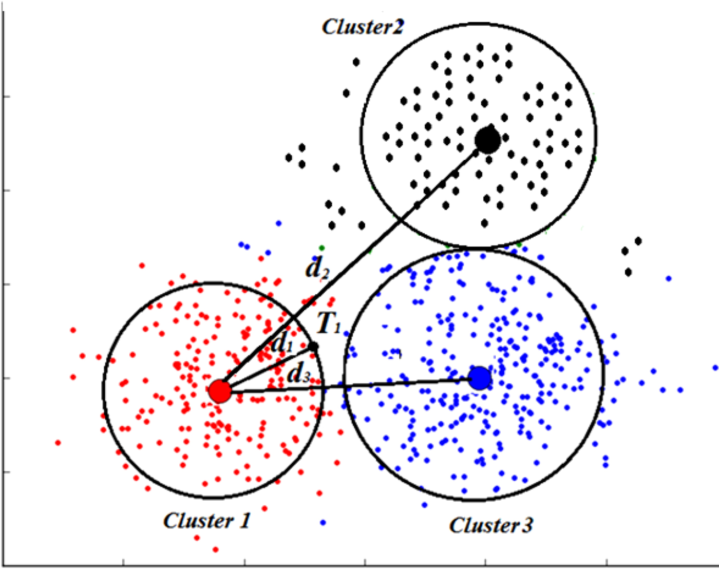
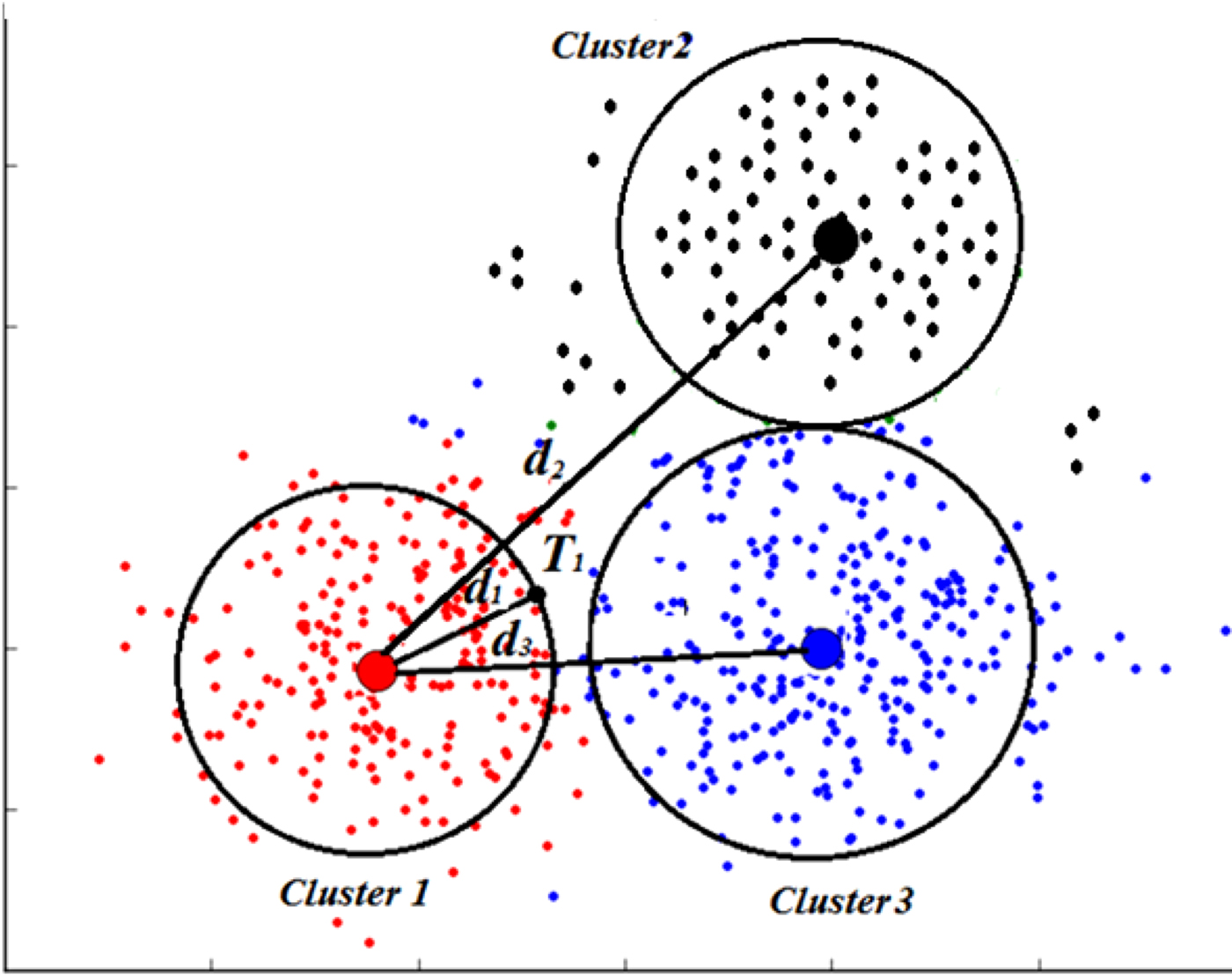
The UFFNN clustering has great capabilities, such as the inherent distributed parallel processing architectures and the ability to adjust the interconnection weights to learn and divide data into meaningful groups. The UFFNN clustering method classifies related data into similar groups without using any class label, and in addition controls noisy data and learns types of input data values based on their weights and properties (Bengio et al., Reference Bengio, Buhmann, Embrechts and Zurada2000; Hegland, Reference Hegland2003; Andonie & Kovalerchuk, Reference Andonie and Kovalerchuk2007; Jain, Reference Jain2010; Rougier & Boniface, Reference Rougier and Boniface2011). In UFFNN clustering, data is divided into meaningful groups with special goals, with related data classified as higher similarities within groups and unrelated data as dissimilarities between groups without using any class label. For example in Figure 1, T 1 shows the maximum threshold of cluster 1, and d shows the distance between two data nodes.
A sample of the distances between the clusters and within each cluster.
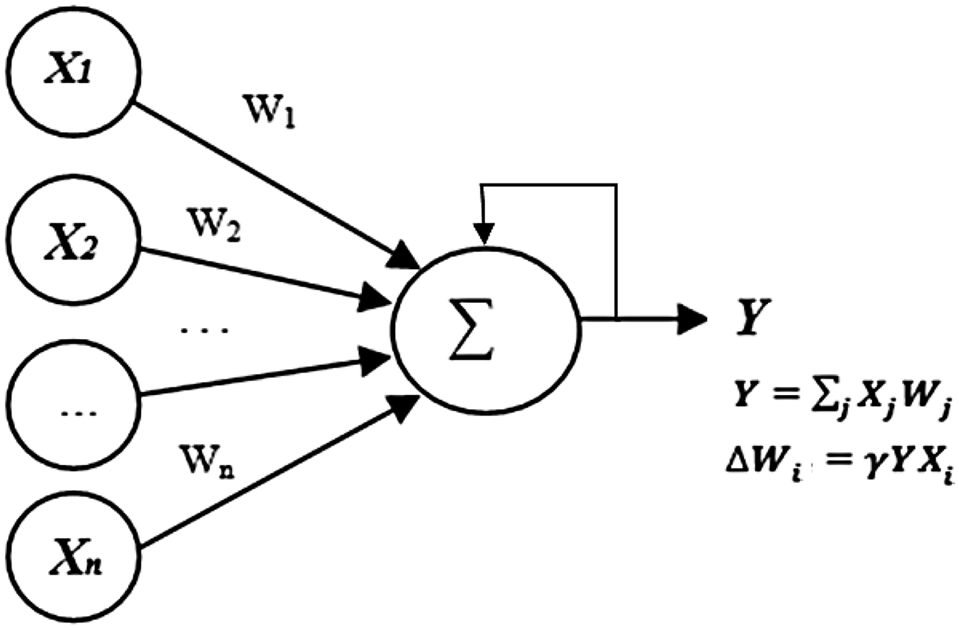
The UFFNN methods often use Hebbian learning, or competitive learning, or competitive Hebbian learning (Martinetz, Reference Martinetz1993; Fritzke, Reference Fritzke1997). Hebb (Reference Hebb1949) developed the meaning of the first learning rule and proposed Hebbian learning. Figure 2 illustrates the single-layer UFFNN as a simple topology with Hebbian learning (Laskowski & Touretzky, Reference Laskowski and Touretzky2006). Hebb described a synaptic flexibility mechanism in which the synaptic connection between two neurons is strengthened, and neuron j becomes more sensitive to the action of neuron i if the latter is close enough to stimulate the former while repeatedly contributing to its activation.
The Hebbian rule is shown in Eq. (1):
 $$\Delta {W_i} = {\rm \gamma} Y{X_i}\comma$$
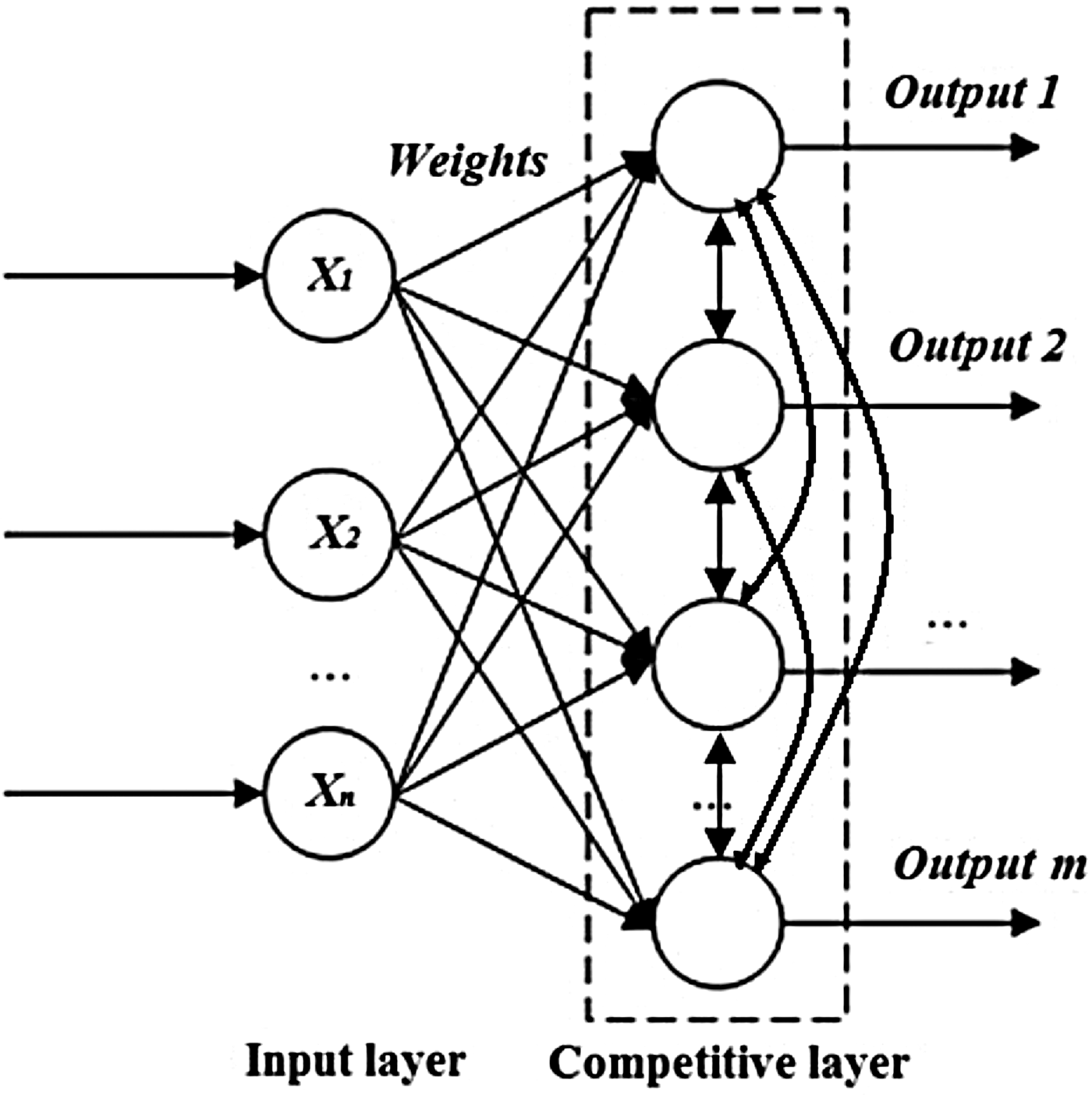
where X is the input vector; Y is the output vector; and γ is the learning rate, where γ > 0 is used to control the size of each training iteration. The competitive learning network is a UFFNN clustering based on learning the nearest weight vector to the input vector as the winner node according to the computing distance, such as Euclidean. Figure 3 shows a sample topology of an unsupervised competitive learning neural network (Haykin & Network, Reference Haykin2004; Du, Reference Du2010).
Single-layer unsupervised feedforward neural network with the Hebbian learning.

A sample topology of the competitive clustering.

The similarities between Hebbian learning and competitive learning include unsupervised learning without error signal, and are strongly associated with biological systems. However, in competitive learning, only one output must be active, such that only the weights of the winner are updated in each epoch. By contrast, no constraint is enforced by neighboring nodes in Hebbian learning, and all weights are updated at each epoch. In the case of competitive Hebbian learning, the neural network method shares some properties of both competitive learning and Hebbian learning. Competitive learning can apply vector quantization (VQ; Linde et al., Reference Linde, Buzo and Gray1980) during clustering. VQ, K-means (Goebel & Gruenwald, Reference Goebel and Gruenwald1999), and some UFFNN clustering methods, such as Kohonen's self-organizing map (SOM; Kohonen, Reference Kohonen1997) and growing neural gas (GNG; Fritzke, Reference Fritzke1995), are generally considered as the fundamental patterns in the current online dynamic UFFNN (ODUFFNN) clustering methods (Asadi et al., Reference Asadi, Sabah Hasan and Abdul Kareem2014b). Linde et al. introduced an algorithm for the VQ design to obtain a suitable code book of weights for input data nodes clustering. VQ is based on probability density functions by distribution of the vector of the weights. VQ divides a large set of the data (vectors) into clusters, each of which is represented by its centroid node, as in the K-means, which is a partitioning clustering method and some other clustering algorithms. The GNG method is an example that uses the competitive Hebbian learning, in which the connection between the winner node and the second nearest node is created or updated in each training cycle. The GNG method can follow dynamic distributions by adding nodes and deleting them in the network during clustering by using the utility parameters. The disadvantages of the GNG include the increase in the number of nodes to obtain the input probability density and the requirement for predetermining the maximum number of nodes and thresholds (Germano, Reference Germano1999; Hamker, Reference Hamker2001; Furao et al., Reference Furao, Ogura and Hasegawa2007; Hebboul et al., Reference Hebboul, Hacini and Hachouf2011). Kohonen's SOM maps multidimensional data onto lower dimensional subspaces, with the geometric relationships between points indicating their similarity. SOM generates subspaces with unsupervised learning neural network training through a competitive learning algorithm. The weights are adjusted based on their proximity to the “winning” nodes, that is, the nodes that most closely resembles a sample input (Ultsch & Siemon, Reference Ultsch and Siemon1990; Honkela, Reference Honkela1998).
1.2. ODUFFNN clustering
The UFFNN methods with online dynamic learning in realistic environments such as astronomy and satellite communications, e-mail logs, and credit card transactions must be improved and have some necessary properties (Kasabov, Reference Kasabov1998; Schaal & Atkeson, Reference Schaal and Atkeson1998; Han & Kamber, Reference Han and Kamber2006; Hebboul et al., Reference Hebboul, Hacini and Hachouf2011). The data in these environments are nonstationary, so ODUFFNN clustering methods should have lifelong (online) and incremental learning. The flexible incremental and dynamic neural network clustering methods are able to do the following (Kasabov, Reference Kasabov1998; Schaal & Atkeson, Reference Schaal and Atkeson1998; Bouchachia et al., Reference Bouchachia, Gabrys and Sahel2007; Hebboul et al., Reference Hebboul, Hacini and Hachouf2011):
• to learn the patterns of high dimensional and huge continuous data quickly; therefore, training should be in one pass. In these environments, the data distributions are not known and may be changed over time.
• to handle new data immediately and dynamically, without destroying old data. The ODUFFNN clustering method should control data, adapt its algorithm, and adjust itself in a flexible style to new conditions of the environment over time dynamically for processing of both data and knowledge.
• to change and modify its structure, nodes, connection, and and so forth with each online input data.
• to accommodate and prune data and rules incrementally, without destroying old knowledge.
• to be able to control time, memory space, accuracy, and so forth efficiently.
• to learn the number of clusters and density of each cluster without predetermining the parameters and rules.
Incremental learning refers to the ability of training in repetition by adding or deleting the data nodes in lifelong learning without destroying outdated prototype patterns (Schaal & Atkeson, Reference Schaal and Atkeson1998; Furao et al., Reference Furao, Ogura and Hasegawa2007; Rougier & Boniface, Reference Rougier and Boniface2011). The ODUFFNN clustering methods should train online data fast without relearning. Relearning during several epochs takes time, and clustering is considerably slow. Relearning affects the clustering accuracy, and time and memory usage for clustering. For the ODUFFNN methods, storing the whole details of the online data and their connection during relearning with the limited memory are impossible. In this case, the topological structure of the incremental online data cannot be represented well, the number of clusters and density of each cluster are not clear, and they cannot be easily learned (Pavel, Reference Pavel2002; Deng & Kasabov, Reference Deng and Kasabov2003; Hinton & Salakhutdinov, Reference Hinton and Salakhutdinov2006; Hebboul et al., Reference Hebboul, Hacini and Hachouf2011). The number of data instances by receiving online data will be grown. This action causes difficulty in clustering, managing the structure of the network and connections between the data, and recognizing the noisy data. Furthermore, clustering of some kinds of data is so difficult because of their character and structure. High feature correlation and the noise in the data cause difficulty in the clustering process, and recognizing the special property of each attribute and finding its related cluster will be difficult. The main disadvantage of dimensionality reduction or feature extraction of data as the data-preprocessing technique is missing values. Missing values are because some important parts of the data are lost, which reflects the accuracy of clustering results (DeMers & Cottrell, Reference DeMers and Cottrell1993; Furao et al., Reference Furao, Ogura and Hasegawa2007; Van der Maaten et al., Reference Van der Maaten, Postma and Van den Herik2009). Therefore, recognizing the special property of each attribute and finding its related cluster will be difficult (Kasabov, Reference Kasabov1998; Hebboul et al., Reference Hebboul, Hacini and Hachouf2011; Rougier & Boniface, Reference Rougier and Boniface2011).
Current ODUFFNN clustering methods often use competitive learning as used in the dynamic SOM (DSOM; Rougier & Boniface, Reference Rougier and Boniface2011), or competitive Hebbian learning as used in the evolving SOM (ESOM). Furao and Hasegawa introduced enhanced self-organizing incremental neural network (ESOINN; Furao et al., Reference Furao, Ogura and Hasegawa2007) based on the GNG method. The ESOINN method has one layer, and in this model, it is necessary that very old learning information is forgotten. The ESOINN model finds the winner and the second winner of the input vector, and then if it is necessary to create a connection between them or to remove the connection. The density, the weight of the winner, and the subclass label of nodes will be updated in each epoch and the noise nodes depending on the input values will be deleted. After learning, all nodes will be classified into different classes. However, it cannot solve the main problems of clustering. Hebboul et al. (Reference Hebboul, Hacini and Hachouf2011) proposed incremental growing with neural gas utility parameter as the latest online incremental unsupervised clustering. The structure is based on the GNG and Hebbian (Hebb, Reference Hebb1949) models, but without any restraint and control on the network structure. The structure of the incremental growing with neural gas utility parameter contains two layers of learning. The first layer creates a suitable structure of the clusters of the input data nodes with lower noise data, and computes the threshold. The second layer uses the output of the first layer in parallel and creates the final structure of clusters. ESOM (Deng & Kasabov, Reference Deng and Kasabov2003) as an ODUFFNN method is based on SOM and GNG methods. ESOM starts without nodes. The network updates itself with online entry, and if necessary, it creates new nodes during one training epoch. Similar to the SOM method, each node has a special weight vector. The strong neighborhood relation is determined by the distance between connected nodes; therefore, it is sensitive to noise nodes, weak connections, and isolated nodes based on Hebbian learning. If the distance is too big, it creates a weak threshold and the connection can be pruned. Figure 4 is an example of this situation (Deng & Kasabov, Reference Deng and Kasabov2003).
An example of the evolving self-organizing map clustering.

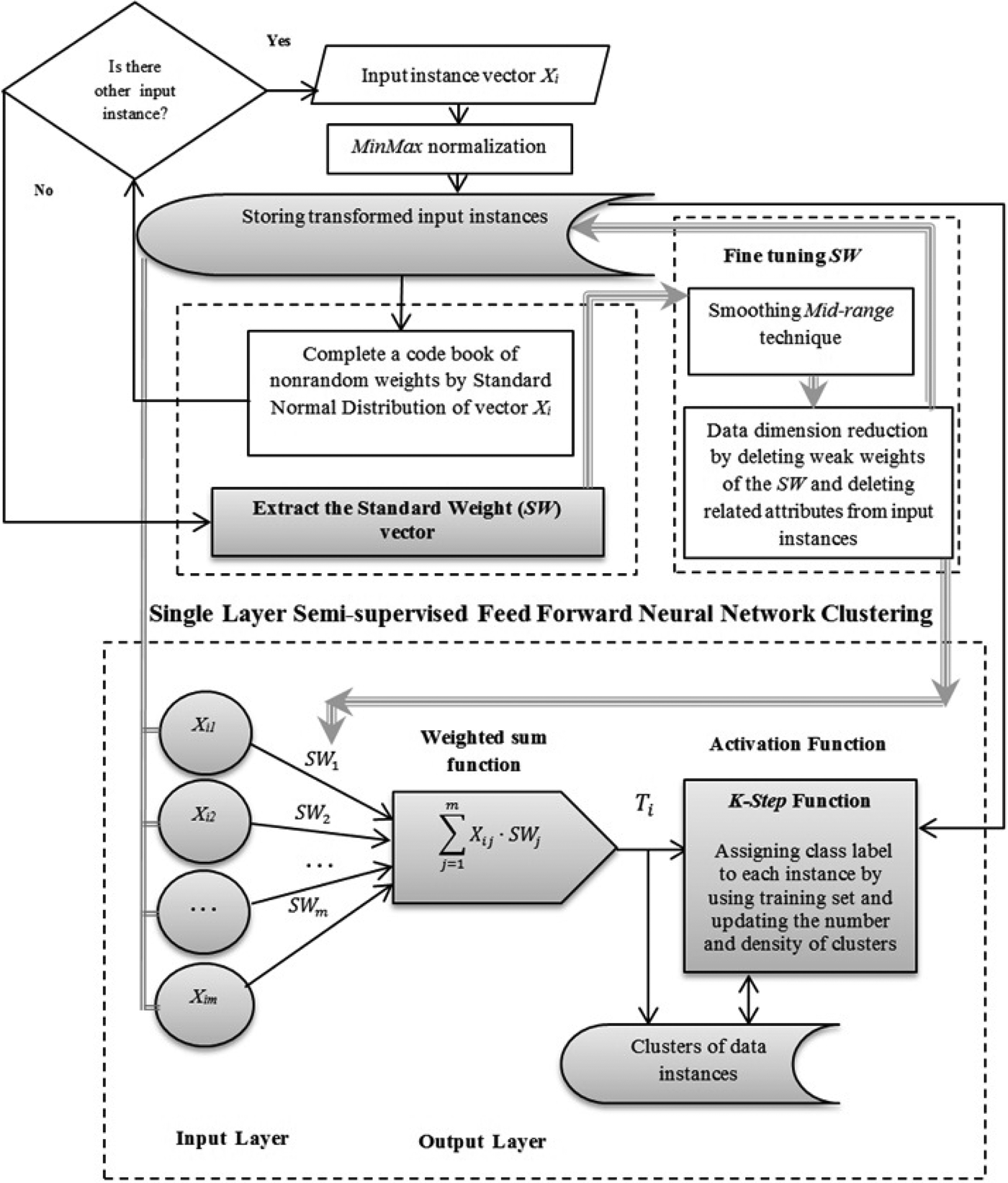
ESOM is a method based on a normal distribution and VQ in its own way, and creates normal subclusters across the data space. DSOM (Rougier & Boniface, Reference Rougier and Boniface2011) is similar to SOM based on competitive learning. In order to update the weights of the neighboring nodes, time dependency is removed, and the parameter of the elasticity or flexibility is considered, which is learned by using trial and error. If the parameter of the elasticity is too high, DSOM does not converge; if it is too low, it may prevent DSOM from occurring and is not sensitive to the relation between neighbor nodes. If no node is close enough to the input values, other nodes must learn according to their distance to the input value. The main critical issues in the ODUFFNN clustering method are low training speed, accuracy, and high memory complexity of clustering (Kasabov, Reference Kasabov1998; Han & Kamber, Reference Han and Kamber2006; Andonie & Kovalerchuk, Reference Andonie and Kovalerchuk2007; Asadi et al., Reference Asadi, Sabah Hasan and Abdul Kareem2014b). Some sources of the problems are associated with these methods. High dimensional data and huge data sets cause difficulty in managing new data and noise, while pruning causes data details to be lost (Kohonen, Reference Kohonen2000; Deng & Kasabov, Reference Deng and Kasabov2003; Hinton & Salakhutdinov, Reference Hinton and Salakhutdinov2006; Van der Maaten et al., Reference Van der Maaten, Postma and Van den Herik2009). Using random weights, thresholds, and parameters for controlling clustering tasks, create the paradox of low accuracy and high training time (Han & Kamber, Reference Han and Kamber2006; Hebboul et al., Reference Hebboul, Hacini and Hachouf2011; Asadi & Kareem, Reference Asadi and Kareem2014). Moreover, the data details and their connections are lost by relearning that affects the CPU time usage, memory usage, and clustering accuracy (Pavel, Reference Pavel2002; Hebboul et al., Reference Hebboul, Hacini and Hachouf2011). Some literature is devoted to improving the UFFNN and ODUFFNN methods by the technique of using constraints such as class labels. The constraints of class labels are based on the knowledge of experts and the user guide as partial supervision for better controlling the tasks of clustering and desired results (Prudent & Ennaji, Reference Prudent and Ennaji2005; Kamiya et al., Reference Kamiya, Ishii, Furao and Hasegawa2007; Shen et al., Reference Shen, Yu, Sakurai and Hasegawa2011). The semi-SOINN (SSOINN; Shen et al., Reference Shen, Yu, Sakurai and Hasegawa2011) and semi-ESOM (Deng & Kasabov, Reference Deng and Kasabov2003), which were developed based on the SOINN and ESOM clustering methods, respectively, are examples in this area. In order to improve the methods, the users manage and correct the number of clusters and density of each cluster by inserting and deleting the data nodes and clusters. After clustering, the models assigned a class label to the winning node and consequently assigned the same class labels to its neighbor nodes in its cluster. Each cluster must have a unique class label; if the data nodes of a cluster have different class labels, the cluster can be divided into different subclusters. However, assigning the class labels to the data nodes between the clusters can be somewhat vague. The judgment of users can be wrong, or they may make mistakes during the insertion, deletion, or finding the link between nodes and assigning the class label to each disjoint subcluster. Asadi et al. (Reference Asadi, Sabah Hasan and Abdul Kareem2014a) applied this technique and introduced a UFFNN method, the efficient real semisupervised FFNN (RSFFNN) clustering model, with one epoch training and data dimensionality reduction ability to overcome the problems of high CPU time usage during training, low accuracy, and high memory complexity of clustering, suitable for stationary environments (Asadi et al., Reference Asadi, Sabah Hasan and Abdul Kareem2014a). Figure 5 shows the design of the RSFFNN clustering method.
The design of the real semisupervised feedforward neural network model for clustering (Asadi et al., Reference Asadi, Sabah Hasan and Abdul Kareem2014a).

The RSFFNN considered a matrix of data set as input data for clustering. During training, a nonrandom weights code book was learned through input data matrix directly, by using normalized input data and standard normal distribution. A standard weight vector was extracted from the code book, and afterward fine-tuning is applied by single-layer FFNN clustering section. The fine-tuning process includes two techniques of smoothing the weights and pruning the weak weights: the midrange technique as a popular smoothing technique is used (Jean & Wang, Reference Jean and Wang1994; Gui et al., Reference Gui, Vasiu and Bojković2001); then, the model prunes the data node attributes with weak weights in order to reduce the dimension of data. Consequently, the single-layer FFNN clustering section generates the exclusive threshold of each input instance (record of the data matrix) based on a standard weight vector. The input instances were clustered on the basis of their exclusive thresholds. In order to improve the accuracy of the clustering results, the model assigns a class label to each input instance by considering the training set. The class label of each unlabeled input instance was predicted by utilizing a linear activation function and the exclusive threshold. Finally, the RSFFNN model updated the number of clusters and density of each cluster. The RSFFNN model illustrated superior results; however, the model must be developed for using as the ODUFFNN clustering method. We introduced an efficient DSFFNN clustering method by developing and modifying the structure of the RSFFNN to overcome the mentioned problems.
2. METHODOLOGY
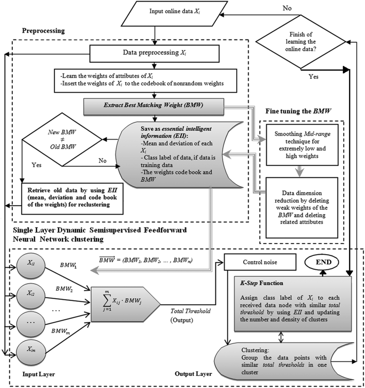
In order to overcome the problems of the ODUFFNN clustering methods as discussed in the last section, we developed the DSFFNN clustering method. For the purposes, the RSFFNN (Asadi et al., Reference Asadi, Sabah Hasan and Abdul Kareem2014a) method as an efficient UFFNN clustering method is structurally improved. Therefore, the DSFFNN model updates its structure, connections, and knowledge through learning the online input data dynamically. The DSFFNN model starts without any random parameters or coefficient value that needs predefinition. Figure 6 shows the design of the DSFFNN clustering method.
The design of the dynamic semisupervised feedforward neural network clustering method.

As shown in Figure 6, the DSFFNN method includes two main sections: the preprocessing section and the single-layer DSFFNN clustering section. In the preprocessing section, the DSFFNN method as an incremental ODUFFNN method considers a part of the memory called essential important information (EII) and initializes the EII by learning the important information about each online input data in order to store and fetch during training, without storing any input data in the memory. The code words of nonrandom weights are generated by training current online input data just in one epoch, and are inserted in the weights code book. Consequently, the unique standard vector is mined from the code book of the weights and stored as the EII in the memory. The single layer of the DSFFNN clustering applies normalized data values, and fetches some information through the EII such as the BMW from the section of the preprocessing and generates thresholds and clusters the data nodes. The topology of the single-layer DSFFNN clustering model is very simple with incremental learning, as shown in Figure 6; it consists of an input layer with m nodes and an output layer with just one node without any hidden layer. The output layer has one unit with a weighted sum function for computing the actual desired output. We generally called the proposed method the DSFFNN clustering method; however, before semisupervised clustering, the model dynamically clusters the data nodes without using any class label. Therefore, we call the clustering phase of the proposed method the dynamic UFFNN (DUFFNN) clustering method. Then in order to improve the accuracy of the result of the DUFFNN clustering, the model applies class labels through using a K-Step activation function. Therefore, we call the proposed model the DSFFNN clustering method.
2.1. Overview of the DSFFNN clustering method
In this section, we illustrate the complete algorithm of the DSFFNN clustering method and explain the details of the proposed clustering method as shown in Figure 6 step by step.
Algorithm: The DSFFNN clustering
Input: Online input data X i;
Output: Clusters of data;
Initialize the parameters:
Let X: Data node domain;
Let newMini: Minimum value of the specific domain of [0, 1] which is zero;
Let newMaxi: Maximum value of the specific domain [0, 1] which is one;
Let i: Current number of the online data node X i;
Let j: Current number of the attribute;
Let X i: ith Current online input data node from domain of X;
Let D: Retrieved old data node from the memory;
Let f: Current number of the received data node;
Let n: Number of received data nodes;
Let m: Number of attributes;
Let W ij: Weight of attribute j of ith current online data node X i;
Let
 $\overrightarrow {\hbox{Prod}} $: A vector of the weights product of each attribute of the weights code book;
Let Prodj: jth component of the
$\overrightarrow {\hbox{Prod}} $ vector which $\overrightarrow {\hbox{Prod}} $ = (Prod1, Prod2, … , Prodm);Let SumBMW: a variable for storing the sum of components of the BMW vector;
Let
$\overrightarrow {\hbox{BMW}} $: Best matching weight vector which $\overrightarrow {\hbox{BMW}} $ = (BMW1, BMW2, … , BMWm);Let BMWj: jth component of the
$\overrightarrow {\hbox{BMW}} $ vector;Let BMWjOld: jth component of the old
$\overrightarrow {\hbox{BMW}} $ vector;Let BMWjNew: jth component of the new
$\overrightarrow {\hbox{BMW}} $ vector;Let T ij: Threshold of attributej of ith current online data node X i;
Let TTi: Total threshold of ith current online data node X i;
Let T fj: Threshold of attributej of fth received data node;
Let TTf: Total threshold of fth received data node;
Method:
While the termination condition is not satisfied
{
Input a new online input data X i;
//1- Preprocessing
// Data preprocessing of X i based on MinMax technique
- $\forall $ j = 1 to m
$$\eqalign{{X_{ij}} & = \left( X_{ij} - {\rm Min}\left(X_{ij}\right) / {\rm Max}(X_{ij}) - {\rm Min}(X_{ij}\right)\big) \cr & \,\quad \times ({\rm newMax} - {\rm newMin}) + {\rm newMin}}$$
// Compute the weight code words of the current online data X i and update the codebook
// Compute the standard normalize distribution (SND) of the current online input data of X i based on μi and σi which are mean and standard deviation of X i:
- $\hskip8pt\forall $ j = 1 to m
{
$$\hskip-110pt\hbox{SND}({X_{ij}}) = ({X_{ij}} - {{\rm \mu} _i})/{{\rm \sigma} _i}\semicolon$$// Consider W ij as weight of X ij equal SND(X ij)
Insert W ij into the weights codebook;$$\hskip-175pt{W_{ij}} = \hbox{SND}({X_{ij}})\semicolon$$// Update
$\overrightarrow {\hbox{Prod}} $ by considering W ij
$$\hskip-140pt\hbox{Prod}_j = \hbox{Prod}_j \times {W_{ij}\semicolon}$$}
// Extracting the BMW vector Extract the global geometric mean vector of the code book of nonrandom weights as the BMW
- $\hskip17pt\forall $ j = 1 to m
$$\hskip-143pt\hbox{BM}{\hbox{W}_j} = \hbox{Pro}{\hbox{d}_j}^{1/a} \semicolon$$$$\hskip-133pt\; \hbox{SumBMW} = \mathop \sum \nolimits_{j = 1}^m \hbox{BM}{\hbox{W}_j}\semicolon$$
- $\hskip18pt\forall $ j = 1 to m
$$\hskip-46pt{{\rm BMW}_j = {\rm Round} \left( \left({\rm BMW}_j / {\rm SumBMW}\right)\comma \ 2 \right)\semicolon}$$
// Update EII Store the weights, mean, and standard deviation of X i as the EII in the memory
{
$$\hskip-92pt{\rm Memory}\left( {{\rm EII}} \right) \leftarrow {\rm Store }\ \left( {{W_{ij}}\comma\ {{\rm \mu }_i}\comma\ {{\rm \sigma }_i}} \right)\semicolon$$$$\hskip-70pt{\rm Memory}\left( {{\rm EII}} \right){\rm } \leftarrow {\rm Store }\ (\overrightarrow {{\rm BMW}} \comma{\rm \; }\overrightarrow {{\rm Prod}} ){\rm }\semicolon$$If X i is from training data and has class label
{
$$\hbox{Memory}\lpar \hbox{EII} \rpar \leftarrow \hbox{Store} \lpar \hbox{class label of}\,{X_i} \rpar $$}
}
//2- Fine-tuning through two techniques
// a) Smooth the components of the BMW vector
- $\hskip29pt\forall $ j = 1 to m
Midrange (BMWj);
// b) Data dimension reduction
Delete attributes with weak weights of the BMWj , that are close to zero;
//3- Single layer DSFFNN clustering
$$\hskip-116pt\hbox{Fetch}\ \lpar {\overrightarrow {\hbox{BMW}}} \rpar \; \leftarrow \hbox{Memory} \lpar {\hbox{EII}} \rpar\semicolon$$// Compute the exclusive total threshold of just X i based on the new BMW
- $\hskip30pt\forall $ j = 1 to m
$$\hskip-87pt\hbox{T}{\hbox{T}_i} = \hbox{T}{\hbox{T}_i} + {X_{ij}} \times \hbox{BM}{\hbox{W}_j}\semicolon$$
If X i is from training data and has class label
{
$$\hbox{Memory}\lpar \hbox{EII} \rpar \leftarrow \hbox{Store} \lpar \hbox{class label of}\,{X_i}\comma\ {\rm TT}_i \rpar \semicolon $$}
// If new BMW is different with old BMW, the model fetches W fj , σf, and μf as the EII from memory and updates thresholds of just the changed attributes, and update the exclusive total threshold of related data point
If
$\lpar \overrightarrow{\hbox{BMW}}_{\rm New} \ne \; \overrightarrow{\hbox{BMW}}_{\rm Old} \rpar ${
- $\hskip29pt\forall $ j = 1 to m
If BMWjNew ≠ BMWjOld
- $\hskip47pt\forall $ f = 1 to n – 1
{
$$\hskip-20pt{\rm Fetch }\ \left( {{W_{\,fj}}\comma\ \,{{\rm \sigma }_f}\comma\ \,{{\rm \mu }_f}} \right) \leftarrow {\rm Memory }\left( {{\rm EII}} \right)\semicolon$$$$\hskip-65pt{D_{fj}} = ({W_{fj}} \times {\sigma _f}) + {\mu _f}\semicolon$$$$\hskip-55pt{T_{\,fj}}_{\rm Old} = {D_{\,fj}} \times \hbox{BM}{\hbox{W}_{\,j{\rm Old}}}\semicolon$$$$\hskip-80ptT{T_f} = T{T_f} - {T_f}_{\rm Old} \semicolon$$$$\hskip-50pt{T_{\,fj}}_{\rm New} = {D_{\,fj}} \times \hbox{BM}{\hbox{W}_{\,j{\rm New}}\semicolon} $$$$\hskip-73ptT{T_{f\;}} = T{T_f} + {T_f}_{\rm New}\semicolon$$}
Memory(EII) ← Update list of thresholds and related class labels;
}
// Recognize and delete noise
Delete isolated input data with solitary thresholds TT;
// DUFFNN clustering
{
Group the data points with similar thresholds (TTi) in one cluster;
Learn and generate optimized number of clusters and their densities;
}
If learning is finished
{
//Improving the result of DUFFNN clustering by using K-step activation function
{
Assign class label to each data node with similar total threshold by using EII;
Prediction the class label to unlabeled data nodes;
Updating the number of clusters and density of each cluster;
}
Output results;
End;
}
Else { Continue to train and cluster next online input data node
}
}





The DSFFNN clustering method involves several phases:
• Preprocessing: Preprocessing is the factor that contributes to the development of efficient techniques to achieve desirable results of the UFFNN clustering such as low training time and high accuracy (Abe, Reference Abe2001; Larochelle et al., Reference Larochelle, Bengio, Louradour and Lamblin2009; Oh & Park, Reference Oh and Park2011; Asadi & Kareem, Reference Asadi and Kareem2014).
The DSFFNN clustering method, contrary to the RSFFNN, applies the preprocessing method that is suitable for online input data preprocessing.
1. Data preprocessing: As shown in Figure 6, the MinMax normalization technique that is suitable for online input data preprocessing and is independent of the other data points (Han & Kamber, Reference Han and Kamber2006; Asadi & Kareem, Reference Asadi and Kareem2014) is considered. The MinMax normalization technique is used to transform an input value of each attribute to fit in a specific range such as [0, 1]. Equation (2) shows the formula of MinMax normalization.
(2)where X ij is the jth attribute value of online input data X i and has special range and domain, where Min(X ij) is the minimum value in this domain and Max(X ij) is the maximum value in this domain; newMini is the minimum value of specific domain of [0, 1], which is equal to zero; and newMaxi is the maximum value of the domain, which is equal to one. After transformation of current online input data, the model continues to learn current data in the next stages.$$\eqalign{ {\rm Normalized}\left( {{X_{ij}}} \right) &= \left( {{X_{ij}} - {\rm Min}\left( {{X_{ij}}} \right)/{\rm Max}\left( {{X_{ij}}} \right) - {\rm Min}\left( {{X_{ij}}} \right)} \right) \cr & \quad \times \left( {{\rm newMax - newMin}} \right) + {\rm newMin}\comma}$$2. Compute the weight code words of the current online data X i and update the codebook: the DSFFNN method creates a code book of nonrandom weights by entering the first online input data and consequently completes the codebook by inserting the code words of each future online input data. In this stage, the proposed model computes the mean μi of the normalized current online input data X i. Then the standard deviation σi of the input data of X i is computed by considering μi. Table 1 provides this information.
Table 1.The online input data X
On the basis of the definition of the SND (Ziegel, Reference Ziegel2002), the SND shows how far each attribute value of the online input data X i is from the mean μi, in the metric standard deviation unit σi. In this step, each normalized attribute value of the online input data X i is considered as the weight W ij for that value. Each element or code word of the weight code book is equal to W ij. Therefore, each weight vector of the codebook is computed based on the SND of each online input data value of X i as shown in Eq. (3).
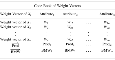
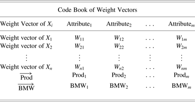
(3)The SND(X ij) is a standard normalized value of each attribute value of the online input data. μi and σi are the mean and standard deviation of X i. Therefore, each SND(X ij) shows the distance of each input value of each data from the mean of the online input data. Accordingly, each W ij as weight of X ij is equal to SND(X ij) as in Eq. (4), and the initialization of weights is not at random:$$\hbox{SND}\lpar {{X_{ij}}} \rpar = {{\lpar {{X_{ij}} - {{\rm \mu}_i}} \rpar } / {{{\rm \sigma} _i}.}}$$(4)The weights of attributes of current input data X i are inserted in the weights code book as the code words of X i. The model considers a vector of the weights as the product of each attribute of the weights code book. The Prod vector consists of the components Prodj for the attributes, which is computed by the product of the weights of each attribute of the code book. The parameter n is the number of received data nodes, which were trained by the model, and i is current number of the online input data node X i; m is the number of attributes, and j is the current number of the attribute. Equations (5) and (6) show these relationships.$$W_{ij} = \hbox{SND}\lpar X_{ij} \rpar \quad i = 1\comma\; 2\comma\;. \;. \;.\;\comma\; n\semicolon\,\; j = 1\comma\; 2\comma\;. \;. \;. \;\comma\; m.$$(5)$$\hbox{Pro}{\hbox{d}_j} = \hbox{Pro}{\hbox{d}_j} \times {W_{ij}\comma} $$(6)$$\; \overrightarrow {\hbox{Prod}} = \lpar {\hbox{Pro}{\hbox{d}_{\rm 1}}\comma\ {\rm Pro}{\hbox{d}_{\rm 2}}\comma\ {\rm \ldots\comma\; Pro}{\hbox{d}_m}} \rpar .$$3. Extracting the BMW vector: In the SOM, the weight of the code book that is nearest to the input vector is distinguished as the winner node and the best matching unit. In the same way, the DSFFNN learns the standard unique weight as BMW. The BMW vector is the global geometric mean (Vandesompele et al., Reference Vandesompele, De Preter, Pattyn, Poppe, Van Roy, De Paepe and Speleman2002; Jacquier et al., Reference Jacquier, Kane and Marcus2003) vector of the code book of the nonrandom weights and is computed based on the gravity center of the current and last trained data nodes. In the DSFFNN method, the codebook of real weights is initialized by considering properties of input values directly and without using any random values or random parameters similar to the RSFFNN clustering method. The RSFFNN computes the standard weight one time through processing of all input data instances in the input matrix; however, the DSFFNN computes the BMW based on the gravity center of the current and last trained data nodes, and with entrance of each online input data, the BMW is updated. The BMW vector is computed by Eqs. (7)–(9) as follows:
(7)$$\hbox{BM}{\hbox{W}_j} = \hbox{Pro}{\hbox{d}_j}^{1/n}\comma $$(8)$${{\rm BM}{{\rm W}_j} = {\rm Round}\left( {\left( {{{{\rm BM}{{\rm W}_j}} / {{\rm SumBMW}}}} \right)\comma\ 2} \right)\comma} $$(9)$${\hbox{SumBMW} = \mathop \sum \nolimits_{\,j = 1}^m \hbox{BM}{\hbox{W}_j}\comma} $$(10)$${\overrightarrow {\hbox{BMW}} = \lpar {\hbox{BM}{\hbox{W}_{\rm 1}}\comma\ {\rm BM}{\hbox{W}_{\rm 2}}\comma\ {\rm \ldots\comma\ BMW}_m} \rpar\comma} $$(11)The parameter n is the number of received data nodes (contain the old data points and current online input data node X i), m is the number of attributes, and j is the current number of attributes. Equation (7) shows the BMWj is the global geometric mean of all W ij of the attributes X i. In Eq. (8), the parameter SumBMW is equal to the sum of the components of the BMW vector. As shown in Eq. (9), the model considers Round function with two digits of each BMWj ratio to SumBMW, because in this way, the model is able to control the changing BMWjNew ratio to BMWjOld. This technique affects the low time and memory complexities of the model. Equation (11) shows the sum of components BMW is equal to one through Eqs. (8) and (9); therefore, we can understand the distribution of amounts of weights between attributes. Table 2 illustrates the code book of the weights and the process of extracting the BMW vector.$${\hbox{Equations} \, \lpar \hbox{8} \rpar \, \hbox{and} \ \lpar \hbox{9} \rpar \Rightarrow \mathop {\rm \sum} \nolimits_{\,j = 1}^m \hbox{BMW}_j = 1}. $$The main goal of the DSFFNN model is learning of the BMW vector as the criterion weight vector. The next stages will show how the threshold of current online data is computed, the current online input data is clustered easily based on the computed BMW vector, and consequently the network of clusters is updated.
4. Update EII: In this stage after learning the weights of attributes of online input data X i, the model stores the mean and standard deviation of X i, computed new BMW and Prod as the EII in the memory. Some data nodes as training data have class labels; therefore, in this phase, if current online input data has a class label, consequently, the model keeps it with other important information of the data in the memory. After clustering, the model will consider the class label and its related total threshold in order to semisupervised clustering of the data in the future stages.
• Fine-tuning: The DSFFNN similar the RSFFNN clustering method applies the techniques of fine-tuning, but after each updating of the BMW process. As Asadi et al. (Reference Asadi, Sabah Hasan and Abdul Kareem2014a) explained, in order to adapt the weights accurately to achieve better results of clustering the data points, two techniques of smoothing the weights and pruning the weak weights can be considered:
1. Smoothing the weights: The speed, accuracy, and capability of the training of the FFNN clustering can be improved, by application of some techniques such as smoothing parameters and weights interconnection (Jean & Wang, Reference Jean and Wang1994; Peng & Lin, Reference Peng and Lin1999; Gui et al., Reference Gui, Vasiu and Bojković2001; Tong et al., Reference Tong, Qi, Wu and Zhou2010). In the Midrange technique as an accepted smoothing technique (Jean & Wang, Reference Jean and Wang1994; Gui et al., Reference Gui, Vasiu and Bojković2001), the average of high weight components of the BMW vector is computed and considered as middle range (Midrange). The input data attributes with too high weight amounts may cause them to dominate the high thresholds and highly effect the clustering results. When some BMWj are considerably higher than other components, the BMWj can be smoothed based on the Midrange smooth technique. If the weights of some components of the BMW are higher than the Midrange, the model will reset their weights to equal the Midrange value.
2. Data dimensionality reduction: The DSFFNN model can reduce the dimension of data by recognizing the weak weights BMWj and deleting the related attributes. The weak weights that are close to zero are less effective on thresholds and the desired output. Hence, the weights can be controlled and pruned in advance.
• Single-layer DSFFNN clustering: The main section of the DSFFNN clustering model is a single-layer FFNN topology to cluster the online data by using normalized values and the components of the BMW vector. The proposed model is able to recluster all old data points by retrieving information from the EII. Two major tasks of the DSFFNN model in this section are to cluster the data points dynamically and after learning to assign class labels and semicluster the data.
• DUFFNN clustering: The DSFFNN clustering carried out during one training iteration is based on nonrandom weights, without any updating weight, activation function, and error function such as mean square error. The threshold or output is computed by using normalized values of the input data node and the fetched BMW vector from EII. When the DSFFNN model learns a huge amount of data for clustering, the new BMW is changed slowly and is close to the last computed BMW. IF components of the new BMWj are equal to the components of the old BMWj, the model just clusters X i. In this case, computing the threshold of each attribute of the current online input data X ij and total threshold of the online input data vector X i are computed by Eqs. (12) and (13).
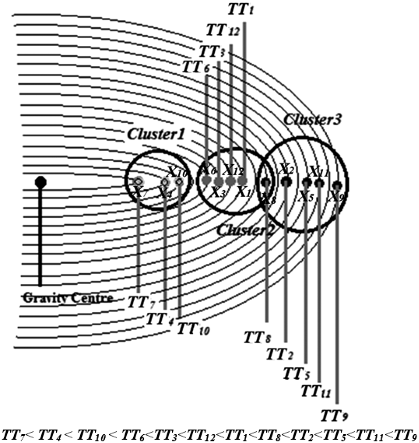
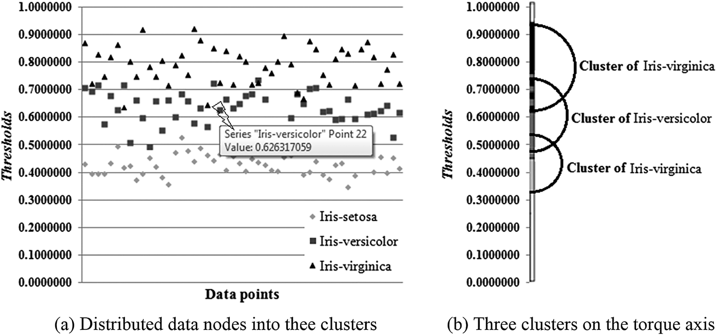
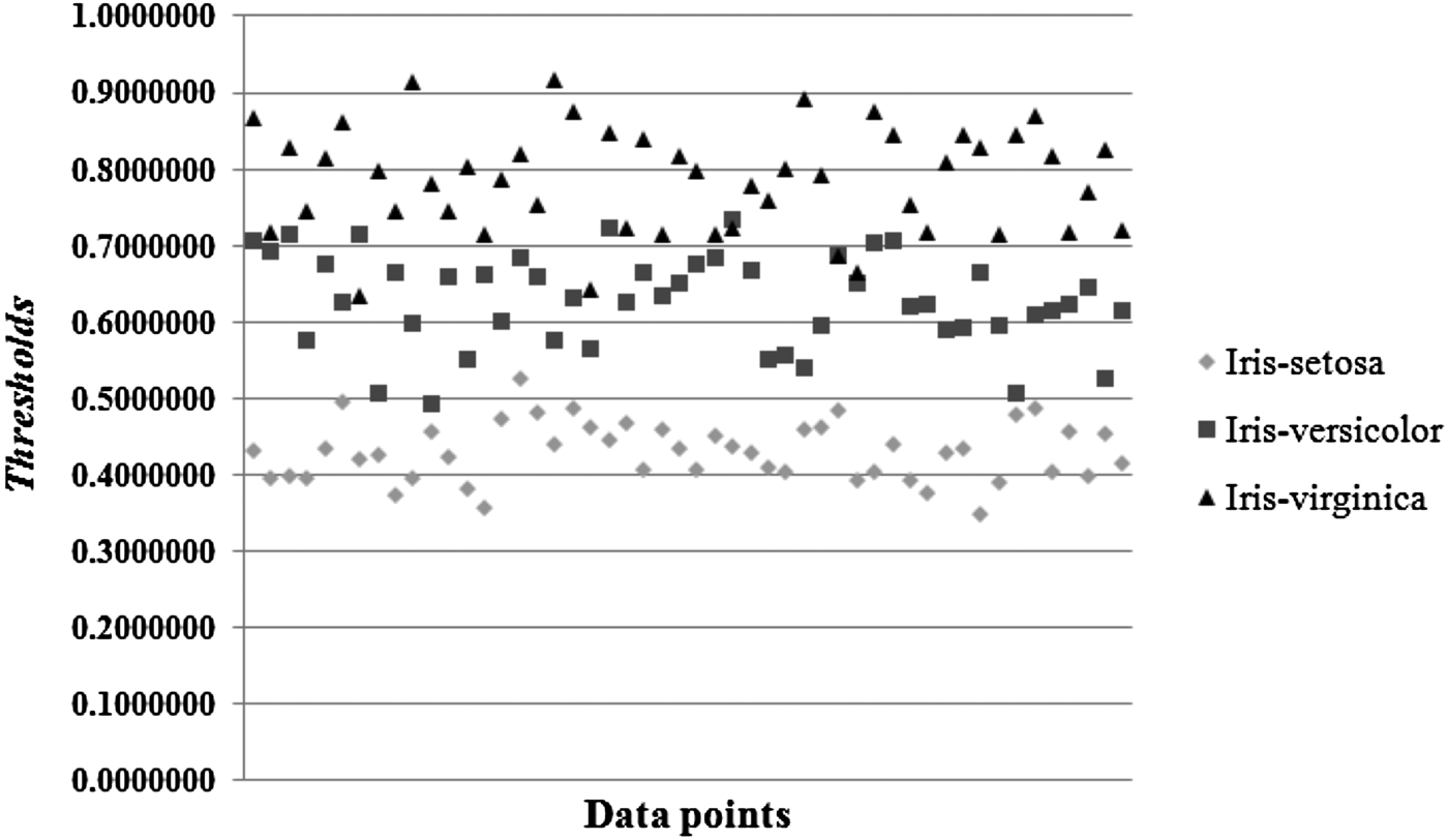
(12)$${T_{ij}} = {X_{ij}} \times \hbox{BM}{\hbox{W}_j}\comma $$(13)$$\hbox{T}{\hbox{T}_i} = \mathop \sum \nolimits_{j = 1}^m {X_{ij}} \times {\rm BMW}_j\quad \hbox{or}\quad \hbox{T}{\hbox{T}_i} = \mathop \sum \nolimits_{j = 1}^m {T_i}\comma $$(14)As Eq. (14) shows, if the current online input data X i has a class label, the DSFFNN model stores the computed total threshold as related TT i to this class label in the memory. During the semisupervised feedforward clustering stage, the model needs this class label. If the new BMW vector is different from the last BMW, the model considers the BMWNew vector based on the feature of Hebbian learning and reclusters all old data points by retrieving information from the EII, based on their related total threshold during one iteration. In this case, the model considers Eqs. (15)–(20), respectively, and checks which components of BMWNew are changed. Consequently, the model fetches the related W fj, σf, μf of each component BMWjOld and retrieves related data node D fj from EII based on Eqs. (3) and (4), and computed related threshold of the data node D fj. By considering the total threshold of the D fj as the EII from the memory and replacing the amounts of old threshold of attribute j of D fj as T fOld and new threshold of attribute j of D fj as T fNew, the data node D fj lies in the special place of axis of the total threshold and suitable cluster.$$\hskip -11pt \hbox{Memory}\lpar {\hbox{EII}} \rpar \ {\rm \leftarrow Store} \lpar {\hbox{Class label of}\,{X_i}\comma\ {\rm T}{\hbox{T}_i}} \rpar {\rm.} $$(15)$$\hbox{Fetch} \lpar {{W_{\,fj}}\comma\ {{\rm \sigma}_f}\comma\ {{\rm \mu}_f}} \rpar {\rm \ \leftarrow Memory}\lpar {\hbox{EII}} \rpar\comma $$(16)$${\hbox{D}_{fj}}= \lpar {{\hbox{W}_{fj}}\times {{\rm \sigma}_f}} \rpar {\rm} + {{\rm \mu} _{f}}\comma $$(17)$${T_f}_{{\rm Old}} = {D_{\,fj}}\times {\rm BM}{\hbox{W}_{\,j{\rm Old}}}\comma $$(18)$${{\rm TT}_f = {\rm TT}_f - {\rm T}_f{\rm Old}}\comma $$(19)$$T_{\,f\,{\rm New}} = D_{fj} \times {\rm BMW}_{j{\rm New}}\comma$$(20)Therefore, it is not necessary to compute and update all thresholds of all old data node attributes. The single-layer DSFFNN computes the total threshold of current input data node X i, updates the total thresholds of old data nodes, and lists thresholds and related class labels. Consequently, the model reclusters all received data nodes. Figure 7 illustrates how the data nodes are clustered by the DSFFNN model.$${\rm TT}_f = {\rm TT}_{f}+ {\rm T}_{f{\rm New}}. $$As shown in Figure 7, each TTi is the total threshold vector of each data point ratio to the gravity center of the data points. Therefore, each data vector takes its own position on the thresholds axis. The online input data X i, based on its exclusive TTi, lies on the axis, respectively. Each data point has an exclusive and individual threshold. If two data points possess an equal total threshold, but are in different clusters, clustering accuracy is decreased because of the error of the clustering method. The DSFFNN considers the data points with close total thresholds into one cluster. Figure 7 is an example of clustering data points into three clusters. Figure 8 is an example of clustering the Iris data points by the DSFFNN clustering. In Figure 8a and b, the Iris data from the UCI repository is clustered to three clusters based on a unique total threshold of each data point by the DSFFNN method. Data point 22 has TT22 = 0.626317059 and lies inside of cluster 2 or the cluster of the Iris Versicolour.
• Pruning the noise: The DSFFNN distinguishes isolated data points through the solitary total thresholds. The total threshold of an isolated data point is not close to the total thresholds of other clustered data points. Therefore, the isolated data point lies out of the locations of other clusters. The proposed DSFFNN method sets apart these data points as noise and removes them. The action of removing the noise causes high speed and clustering accuracy with low memory usage of the network in big data sets.
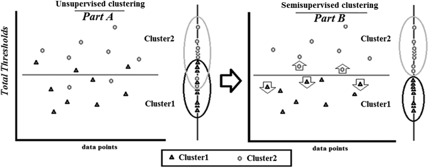
• Improving the result of the DUFFNN clustering by using K-step activation function: As mentioned in Section 1, there is a technique of converting a clustering method to semisupervised clustering by considering some constraint or user guides as feedback from users. K-step activation function (Alippi et al., Reference Alippi, Piuri and Sami1995) or threshold function is a linear activation function for transformation of input values. This kind of function is limited with K values based on the number of classes of the data nodes, and each limited domain of thresholds refers to the special output value of the K-step function. The binary-step function is a branch of the K-step function for two data classes 0 and 1. It is often used in single-layer networks. The function g(TTi) is the K-step activation function for the transformation of TTi and output will be 0 or 1 based on the threshold TTi. After clustering the data node by the DUFFNN, the proposed method considers the class label as a constraint in order to improve the accuracy of the result of clustering. If the current online input data X i is a training data and has a class label, the model fetches the class label and related total threshold of X i from memory as EII and assigns this class label to the data nodes with similar threshold and updates the data nodes by using the K-step function. Consequently, based on K class labels and related exclusive thresholds in the EII, the proposed method expects K clusters and for each cluster considers a domain of thresholds. By considering the cluster results of the last phase, if there are some data points with a related threshold in each cluster but without a class label (unknown or unobserved data), the model supposes that these data nodes have the same class label as their clusters. During the process of future online data nodes, when the model updates data nodes, the class labels of these unknown data nodes will be recognized and adjusted for the suitable cluster if necessary. Hence, the class label of unknown data is predicted in two ways: during clustering by considering the related cluster, which the data lies in there, and by using the K-step function based on relationships between thresholds and class labels in the EII. Therefore, the DSFFNN clustering method similar to the RSFFNN applies the “trial and error” method, in order to predict the class label for the unobserved data. The class label of each unknown observation is signed and predicted based on the K-step function and the related cluster and thresholds domain of the cluster where the input instance is. The accuracy of the results of the DSFFNN clustering is measured by F-measure function with 10-fold cross-validation, and the accuracy will show the validation of the prediction. Furthermore, the method updates the number of clusters and the density of each cluster by using class labels. Figure 9 shows an example for clustering a data set to two clusters (Part A), and improving the result by DSFFNN clustering (Part B).


An example for clustering the data nodes to three clusters by the dynamic semisupervised feedforward neural network.

The outlook of clustering the online Iris data to three clusters based on a unique total threshold of each data point by the dynamic semisupervised feedforward neural network.

The outlook of the dynamic semisupervised feedforward neural network clustering method.

The code book of the weight vectors and the BMW vector
3. EXPERIMENTAL RESULTS AND COMPARISON
All of the experiments were implemented in Visual C#.Net in Microsoft Windows 7 Professional operating system with a 2 GHz Pentium processor. To evaluate the performance of the DSFFNN clustering model, a series of experiments on several related methods and data sets were used.
3.1. Data sets from UCI Repository
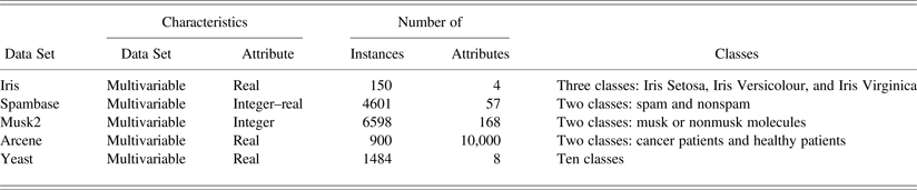
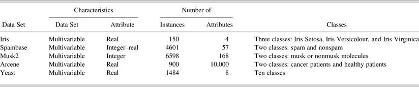
The Iris, Spambase, Musk2, Arcene, and the Yeast data sets from the University of California at Irvine (UCI) Machine Learning Repository (Asuncion & Newman, Reference Asuncion and Newman2007) are selected for evaluation of the proposed model as shown in Table 3. As mentioned in the UCI Repository, the data sets are remarkable because most conventional methods do not process well on these data sets. The type of the data set is the source of clustering problems, such as estimation of the number of clusters and the density of each cluster; or in other words, recognizing similarities of the objects and relationships between attributes of the data set. Large and high-dimensional data creates some difficulties of clustering, especially in real dynamic environments, as mentioned in the Section 1. For experimentation, the speed of processing was measured by the number of epochs. The accuracy of the methods is measured through the number of clusters and the quantity of correctly classified nodes (CCNs), which shows the total nodes and density with the correct class in the correct related cluster in all clusters created by the model. The CCNs are the same as the true positive and true negative nodes. Furthermore, the accuracy of the proposed method is measured by F-measure function for 10-folds of the test set. The precision of computing was considered with 15 decimal places for more dissimilar threshold values. For simulation of the online real environment, every time just one instance of the training or test data is selected randomly and is processed by the models.
The information of selected data sets in this study from the UCI Repository
3.1.1. Iris data set
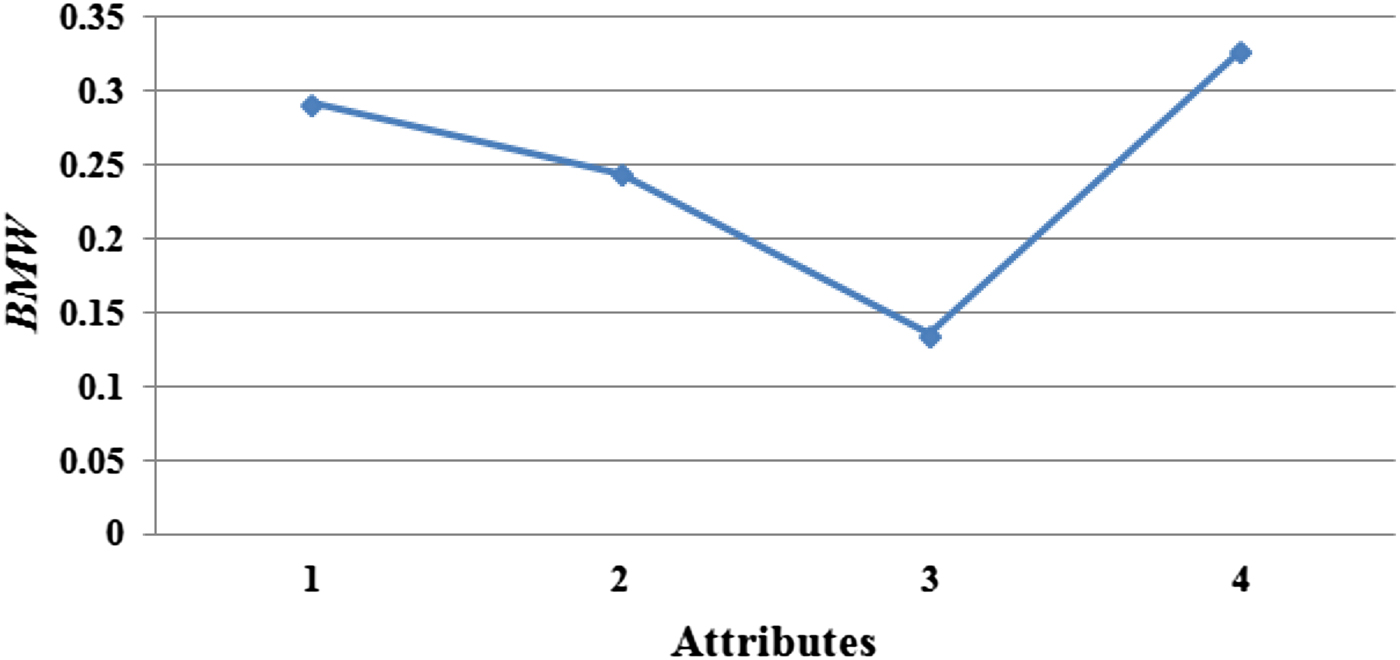
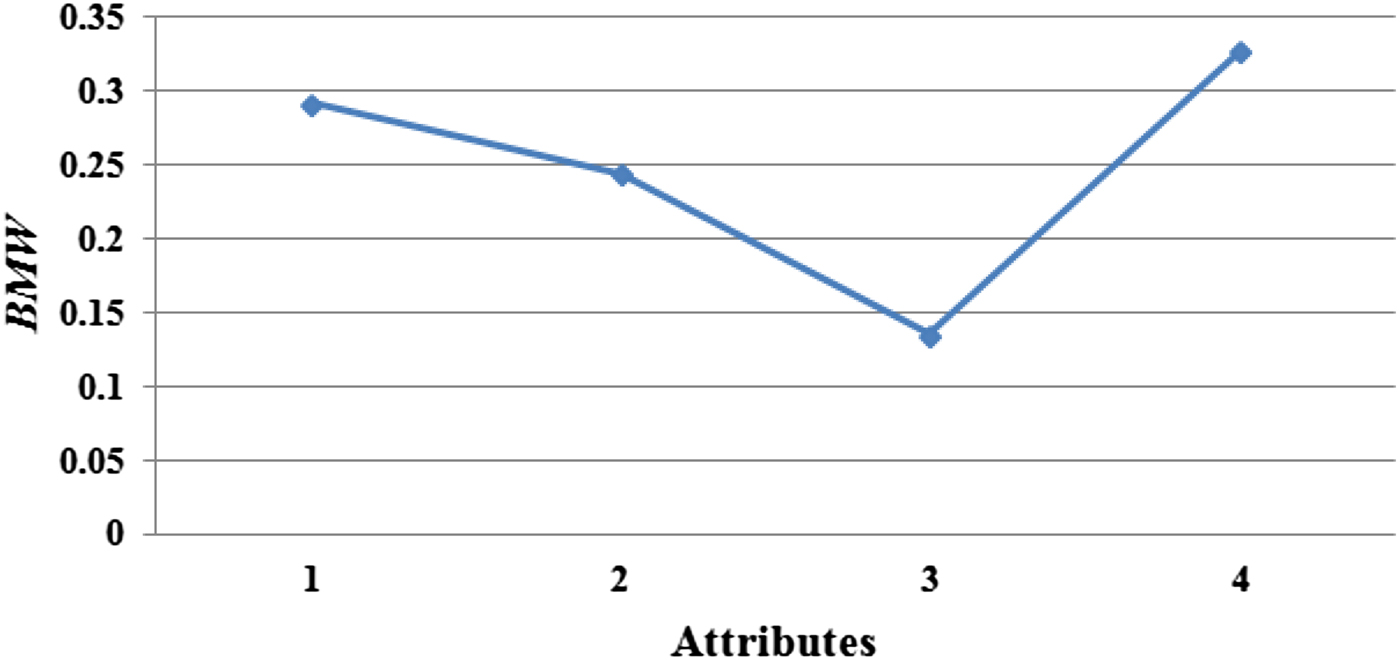
The Iris plants data set was created by Fisher (Reference Fisher1950; Asuncion & Newman, Reference Asuncion and Newman2007). The Iris can be classified into Iris Setosa, Iris Versicolour, and Iris Virginica. Figure 10 shows the final computed BMW vector of the received Iris data points by the DSFFNN clustering method.
The final computed best matching weight vector components of the received Iris data by using the dynamic unsupervised feedforward neural network method.
The total thresholds of the received Iris data were computed on the basis of the final BMW vector. As shown in Figure 11, three clusters can be recognized.
The clusters of the received data points from the Iris data by using the dynamic unsupervised feedforward neural network method.

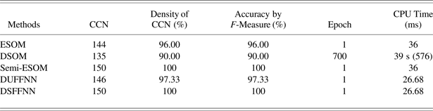
Table 4 shows the comparison of the results of the proposed DSFFNN method with the results of some related methods for the Iris data (Asadi et al., Reference Asadi, Sabah Hasan and Abdul Kareem2014a, Reference Asadi, Sabah Hasan and Abdul Kareem2014b). As shown in Table 4, the ESOM clustered the Iris data points with 144 CCNs, 96.00% density of the CCNs and 96.00% accuracy by the F-measure after 1 epoch during 36 ms. The DSOM clustered the data points with 135 CCNs and 90.00% density of the CCNs and 90.00% accuracy by the F-measure after 700 epochs during 39 s and 576 ms. The semi-ESOM clustered the Iris data points with 150 CCNs, 100% density of the CCNs and 100% accuracy by the F-measure. The DUFFNN clustering method clustered this data set with 146 CCNs, 97.33% density of the CCNs and 97.33% accuracy by F-measure. The BPN, as a supervised FFNN classification model, learned this data set after 140 epochs with the accuracy of 94.00% by using F-measure. As Table 4 shows, the DUFFNN clustering method has superior results. All clustering methods show three clusters for this data set. In order to get a better result of the DUFFNN clustering method, we implemented the DSFFNN by using the Iris data. The results of the DSFFNN show 150 CCNs, 100% density of the CCNs and 100% accuracy by F-measure with 1 epoch for training just during 26.68 ms.
Comparison of the clustering results on the Iris data points by the DSFFNN and some related methods

3.1.2. Spambase data set
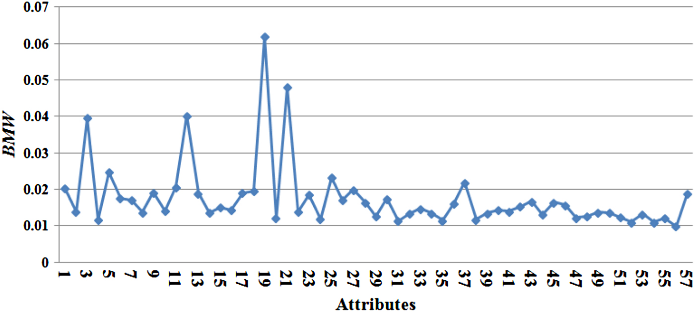
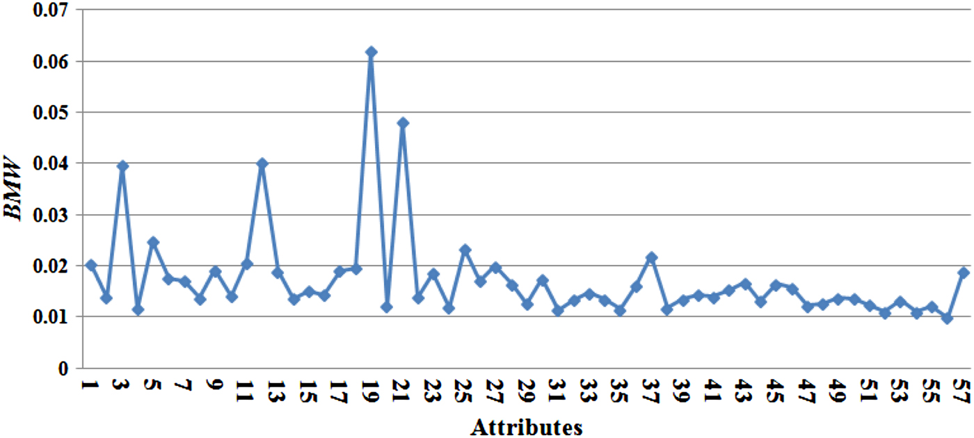
The Spambase E-mail data set is created by Mark Hpkins, Erik Reeber, George Forman, and Jaap Suermondt (Asuncion & Newman, Reference Asuncion and Newman2007). The Spambase data set can be classified into spam and nonspam. Figure 12 shows the final computed BMW vector of the received Spambase data by the DSFFNN clustering method.
The final computed best matching weight vector components of the received Spambase data by using the dynamic supervised feedforward neural network method.
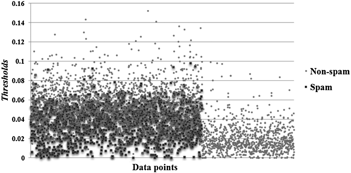
The total thresholds of input data were computed based on the BMW vector. Consequently, the input data were clustered. As shown in Figure 13, two clusters are recognized.
The clusters of the received data points of the Spambase data by using the dynamic supervised feedforward neural network method.

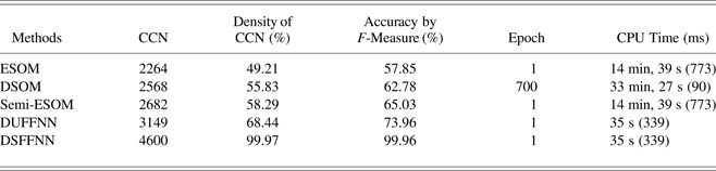
Table 5 shows the comparison of the results of the proposed DSFFNN method with the results of some related methods for the Spambase data (Asadi et al., Reference Asadi, Sabah Hasan and Abdul Kareem2014a, Reference Asadi, Sabah Hasan and Abdul Kareem2014b). As shown in Table 5, the ESOM clustered the Spambase data points with 2264 CCNs, 49.21% density of the CCNs and 57.85% accuracy by the F-measure after 1 epoch during 14 min, 39 s, and 773 ms. The DSOM clustered the data points with 2568 CCNs and 55.83% density of the CCNs and 62.78% accuracy by the F-measure after 700 epochs during 33 min,, 27 s, and 90 ms. The semi-ESOM clustered the Spambase data points with 2682 CCNs, 58.29% density of the CCNs and 65.03% accuracy by the F-measure. The DUFFNN clustering method clustered this data set with 3149 CCNs, 68.44% density of the CCNs and 73.96% accuracy by F-measure after 1 epoch during 35 s and 339 ms. The BPN learned this data set after 2000 epochs with the accuracy of 79.50% by using F-measure. As Table 5 shows, the DUFFNN clustering method has superior results. All clustering methods show two clusters for this data set. The results of the DSFFNN show 4600 CCNs, 99.97% density of the CCNs and 99.96% accuracy by F-measure with 1 epoch for training.
Comparison of the clustering results on the Spambase data points by the DSFFNN and related methods

3.1.3. Musk2 data set
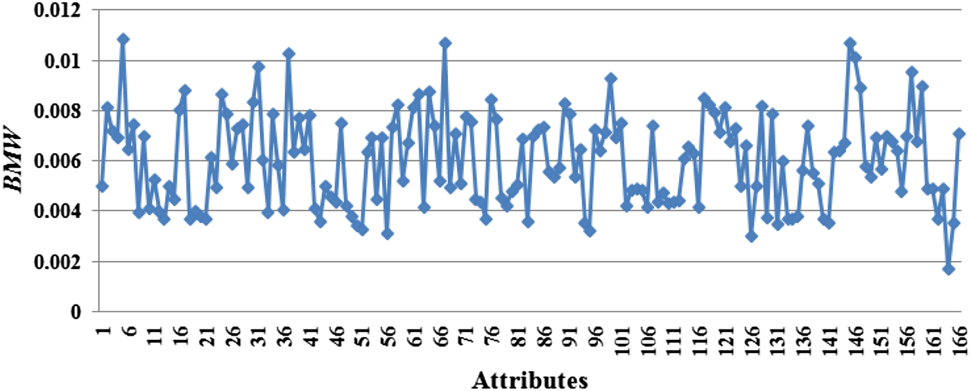
The Musk2 data set (version 2 of the musk data set) is selected from the UCI Repository. The data set was created by the Artificial Intelligence group at the Arris Pharmaceutical Corporation, and describes a set of musk or nonmusk molecules (Asuncion & Newman, Reference Asuncion and Newman2007). The goal is to train to predict whether new molecules will be musk or nonmusk based on their features. Figure 14 shows the final computed BMW vector of the received Musk2 data by the DSFFNN clustering method.
The final computed best matching weight vector components of the received Musk2 data by using the dynamic supervised feedforward neural network method.
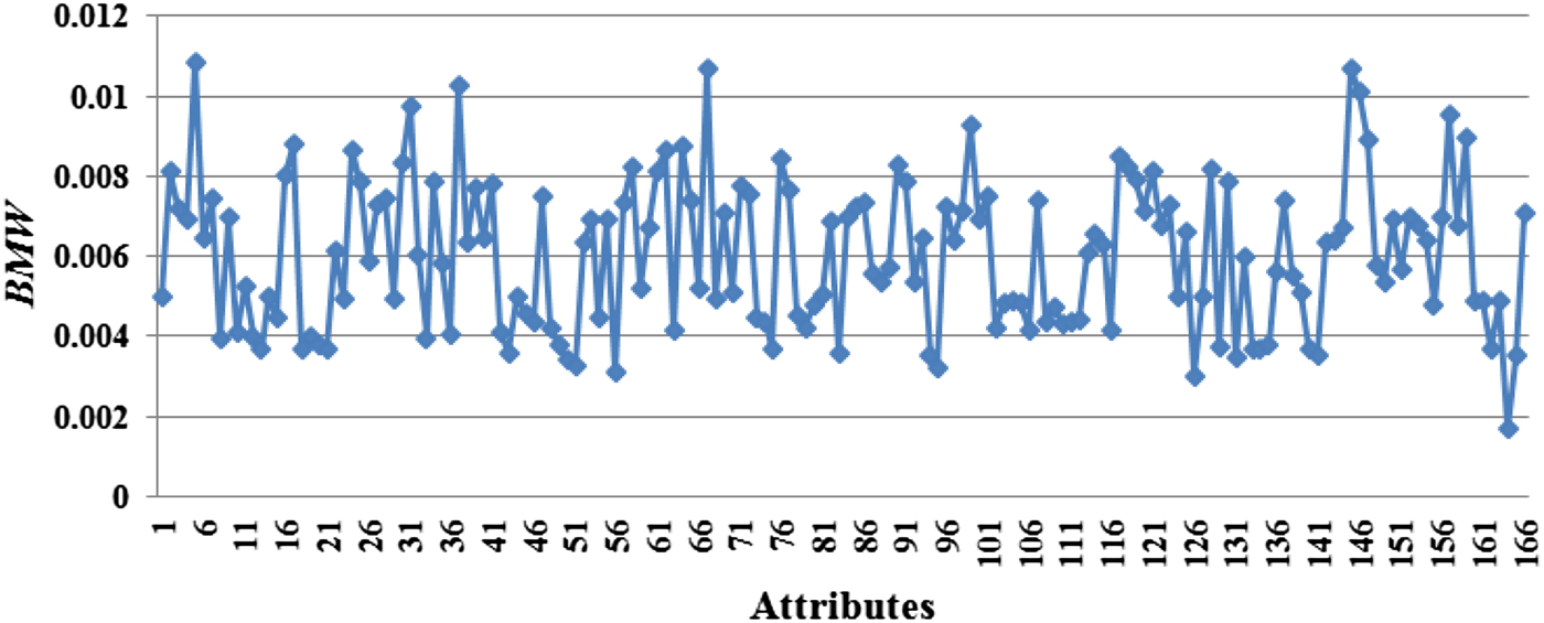
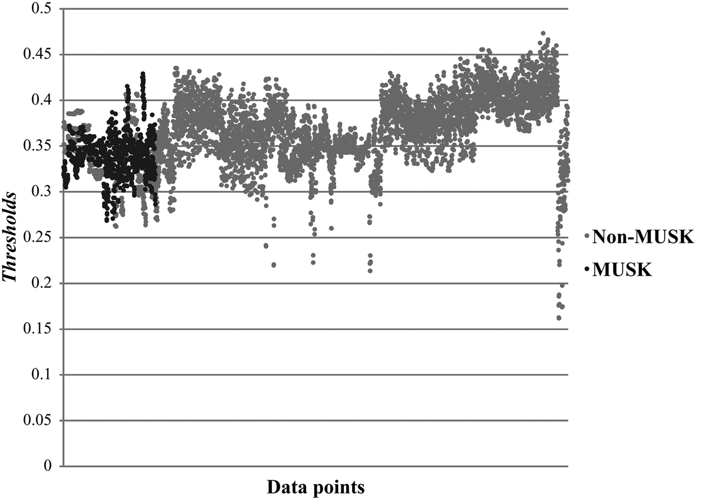
The total thresholds of input data were computed based on the BMW vector. Consequently, the input data were clustered. As shown in Figure 15, two clusters are recognized.
The clusters of the received data points from the Musk2 data by the dynamic supervised feedforward neural network method.

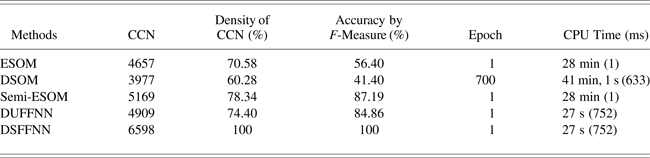
Table 6 shows the comparison results of the proposed DSFFNN method with the results of some related methods for the Musk2 data (Asadi et al., Reference Asadi, Sabah Hasan and Abdul Kareem2014a, Reference Asadi, Sabah Hasan and Abdul Kareem2014b). As Table 6 shows, the ESOM clustered the Musk2 data set with 4657 CCNs, 70.58% density of the CCNs and 56.40% accuracy by F-measure after 1 epoch during 28 min and 1 ms. The DSOM clustered the Musk2 data set with 3977 CCNs, 60.28% density of the CCNs and 41.40% accuracy by F-measure after 700 epoch during 41 min, s, and 633 ms. The semi-ESOM clustered the Musk2 data set with 5169 CCNs, 78.34% density of the CCNs and 87.19% accuracy by F-measure. The DUFFNN clustering method clustered this data set with 4909 CCNs, 74.40% density of the CCNs and 84.86% accuracy by F-measure after 1 epoch during 27 s and 752 ms. The BPN learned this data set after 100 epochs with 67.00% accuracy by F-measure. All clustering methods show two clusters for this data set. The results of the DSFFNN show 6598 CCNs, 100% density of the CCNs and 100% accuracy by F-measure.
Comparison of the clustering results on the Musk2 data points by the DSFFNN and some related methods

3.1.4. Arcene data set
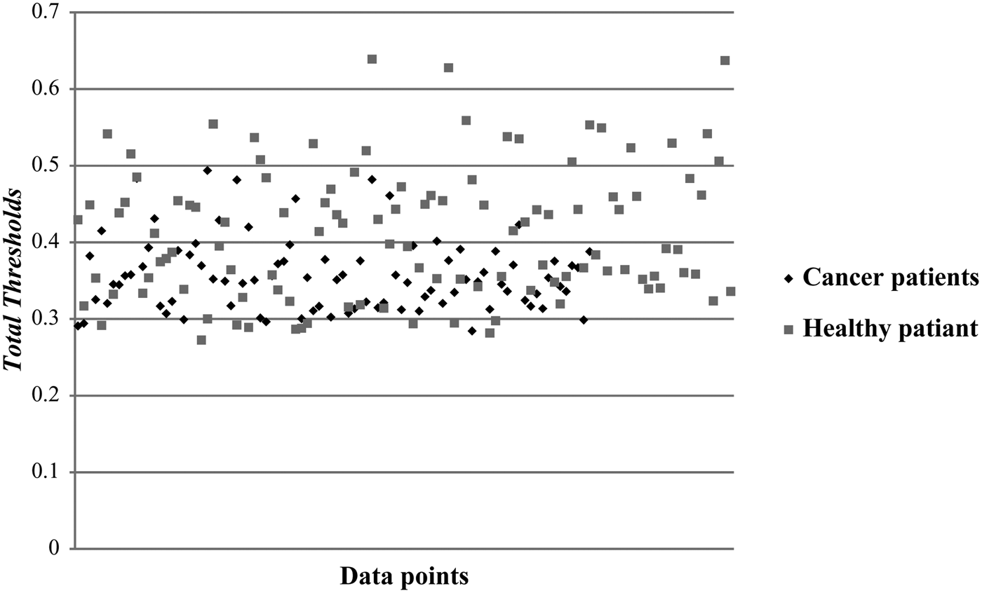
The Arcene data set was collected from two different sources: the national cancer institute and the eastern Virginia medical school (Asuncion & Newman, Reference Asuncion and Newman2007). All data were earned by merging three mass-spectrometry data sets to create training and test data as a benchmark. The training and validation instances include patients with cancer (ovarian or prostate cancer) and healthy patients. Each data set of training and validation contains 44 positive samples and 56 negative instances with 10,000 attributes. We considered the training data set and validation data set with 200 total instances together as one set. The Arcene data set can be classified into cancer patients and healthy patients. Arcene's task is to distinguish cancer versus normal patterns from mass-spectrometric data (Asuncion & Newman, Reference Asuncion and Newman2007). This data set is one of five data sets of the Neural Information Processing Systems 2003 feature selection challenge (Guyon, Reference Guyon2003; Guyon & Elisseeff, Reference Guyon and Elisseeff2003). Therefore, most current existing papers are subject to the best selection of attributes in order to reduce the dimension of the arcane data set with better accuracy, CPU time usage, and memory usage. In this research, we cluster the Arcene data by using the DUFFNN and the DSFFNN clustering methods with just fine-tuning without selection of special attributes. After final updating of the codebook of nonrandom weights and extracting final BMW, Figure 16 shows two clusters of the received data points from the Arcene data was recognized by the DUFFNN clustering method.
The clusters of the received data points of the Arcene data by using the dynamic supervised feedforward neural network method.

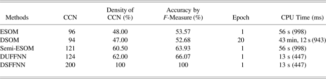
Table 7 shows the comparison the proposed DSFFNN method with some related methods for the Arcene data. The ESOM clustered the Arcene data set with 96 CCNs, 48.00% density of the CCNs and 53.57% accuracy by F-measure after 1 epoch during 56 s and 998 ms. The DSOM clustered the Arcene data set with 94 CCNs, 47.00% density of the CCNs and 52.68% accuracy by F-measure after 20 epochs during 43 min, 12 s, and 943 ms. The semi-ESOM clustered the Arcene data set with 121 CCNs, 60.50% density of the CCNs and 63.93% accuracy by F-measure. The DUFFNN clustering method clustered this data set with 124 CCNs, 62.00% density of the CCNs and 66.07% accuracy by F-measure after 1 epoch just during 13 s and 447 ms. All clustering methods show two clusters for this data set. The results of the DSFFNN show 200 CCNs, 100% density of the CCNs and 100% accuracy by F-measure. The DSOM is not a suitable method to implement for clustering of this data set through its time and memory complexities. Recently, Mangat and Vig (Reference Mangat and Vig2014) reported classification of the Arcene data set by several classification methods such as K-nearest neighbor (K-NN). K-NN is a supervised classifier that is able to learn by analogy and performs on n-dimensional numeric attributes (Dasarthy, Reference Dasarthy1990). Given an unknown instance, K-NN finds K instances in the training set that are closest to the given instance pattern and predicts one or an average of class labels or credit rates. Unlike BPN, K-NN assigns equal weights to the attributes. The K-NN (K = 10) was able to classify the Arcene data set with 77.00% accuracy by F-measure after several epochs and 10 times running the method. Comparison of the results of the DSFFNN clustering method with the results of other related methods shows the superior results of the DSFFNN clustering method.
Comparison of the clustering results on the Arcene data points by the DSFFNN and some related methods

3.1.5. Yeast data set
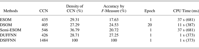
The Yeast data set is obtained from the UCI Repository. The collected data set is reported by Kentai Nakai from the Institute of Molecular and Cellular Biology, University of Osaka (Asuncion & Newman, Reference Asuncion and Newman2007). The aim is to predict the cellular localization sites of proteins. The Yeast data set contains 1484 samples with eight attributes. The classes are cytosolic, nuclear, mitochondrial, and membrane protein: no N-terminal signal, membrane protein: uncleaved signal and membrane protein: cleaved signal. Extracellular, vacuolar, peroxisomal, and endoplasmic reticulum lumen (Asuncion & Newman, Reference Asuncion and Newman2007). In this research, we cluster the Yeast data by using the DSFFNN clustering method taking 1 s and 373 ms training time. Table 8 shows the speed of processing based on the number of epochs and the accuracy based on the density of the CCNs in the Yeast data set by the DSFFNN method.
Comparison of the clustering results on the Yeast data points by the DSFFNN and some related methods

In Table 8, based on the results of the experiment, the ESOM clustered the Yeast data with 435 CCNs, 29.31% density of the CCNs and 17.63% accuracy by F-measure after 1 epoch during 37 s and 681 ms. The DSOM clustered the Yeast data with 405 CCNs, 27.29% density of the CCNs and 24.53% accuracy by F-measure after 20 epoch during 11 s and 387 ms. The semi-ESOM clustered this data with 546 CCNs, 36.79% density of the CCNs and 20.72% accuracy by F-measure. The DUFFNN clustering method clustered this data set with 426 CCNs, 28.71% density of the CCNs and 27.25% accuracy by F-measure after 1 epoch just during 1 s and 373 ms. The DSFFNN clustering method clustered this data set with 1484 CCNs, 100% density of the CCNs and also by F-measure. Several studies reported the difficulty of clustering or classification of the Yeast data set. As Longadge et al. (Reference Longadge, Dongre and Malik2013) reported, classification of the Yeast data set was done by several classification methods such as K-NN. The K-NN (K = 3) was able to classify the Yeast data set with 0.11% accuracy by F-measure after several epochs and times running the method. In addition, Ahirwar (Reference Ahirwar2014) reported the K-means was able to classify the Yeast data set with 65.00% accuracy by F-measure after several epochs.
3.2. Prediction of clathrate hydrate temperature
Clathrate hydrates or gas hydrates are crystalline water-based solids that physically appear like ice. In clathrate hydrates, molecules such as gases form a framework that traps other molecules. Otherwise, the grille structure of the clathrate hydrate breaks into formal ice crystal structure or liquid water. For example, the low molecular weight gases, such as H2, O2, N2, CO2, and CH2, often form hydrates at suitable temperatures and pressures. Cathrate hydrates are not formally chemical compounds, and their formation and decomposition are first-order phase transitions. The details of the formation and decomposition mechanisms at a molecular level are still critical issues to research. In 1810, Humphry Davy (Reference Davy1811) investigated and introduced the clathrate hydrate. In hydrate studies, two main areas have attracted the attention: prevention or elimination of hydrate formation in pipelines, and feasibility examination of the gas hydrate technological applications. In studying any of these areas, the issue that should be addressed first is hydrate thermodynamic behavior. For example, thermodynamic conditions of the hydrate formation are often detected in pipelines, because the clathrate crystals can be accumulated and plug the line. Many researchers have tried to prognosticate this phenomena by using various predictive methods and understanding the conditions of hydrate formation (Eslamimanesh, Reference Eslamimanesh, Mohammadi and Richon2012; Ghavipour, Reference Ghavipour, Ghavipour, Chitsazan, Najibi and Ghidary2013; Moradi, Reference Moradi, Nazari, Alavi and Mohaddesi2013). One of these methods is a hydrate formation temperature estimation by applying neural network methods (Kobayashi et al., Reference Kobayashi, Song and Sloan1987; Shahnazar & Hasan, Reference Shahnazar and Hasan2014; Zahedi et al., Reference Zahedi, Karami and Yaghoobi2009).
Kobayashi et al. (Reference Kobayashi, Song and Sloan1987) selected six different specific gravities and experimentally considered the relationship between the variables of pressure and temperature of gas when the clathrate hydrate is formed. They collected 203 data points, with 136 data points as a training set and 67 data points as a test set. Zahedi et al. (Reference Zahedi, Karami and Yaghoobi2009) applied a multilayer perceptron neural network classification model with seven hidden layers, in the Matlab neural network toolbox (Mathworks, 2008), to predict hydrate formation temperature for each operating pressure, and compared their results with the results of statistical methods by Kobayashi et al. (Reference Kobayashi, Song and Sloan1987). Their results showed that their neural network method had better results.
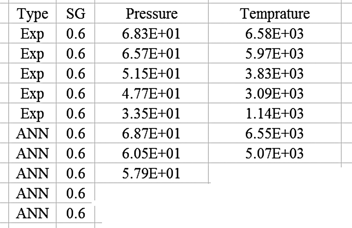
In order to evaluate the DUFFNN model performance, a data set with 299 experimental data points in a temperature range of 33.7–75.7°F and a pressure of 200–2680.44 psi are considered (Shahnazar & Hasan, Reference Shahnazar and Hasan2014). Figure 17 shows a sample of this data set.
A sample of the clathrate hydrate formation data set.

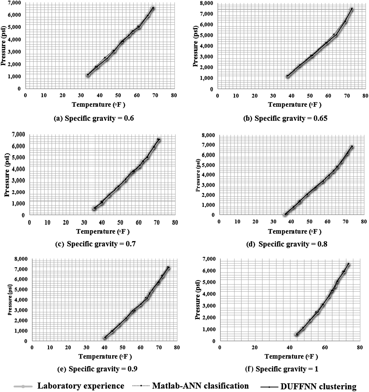
The DUFFNN clustering results are compared with the ANN classification result of Zahedi et al. (Reference Zahedi, Karami and Yaghoobi2009), and laboratory experimental results of Kobayashi et al. (Reference Kobayashi, Song and Sloan1987), which is available in the literature, as shown in Figure 18.
Comparison of the laboratory experience with the results of the Matlab–artificial neural network classification and the dynamic unsupervised feedforward neural network clustering methods.

Figure 18 shows that the result of the DUFFNN clustering is closer than the Matlab-ANN classification to the laboratory experience. The DUFFNN clustering model proved to predict the hydrate formation temperature with more than 98% accuracy. Therefore, the results of Figure 18 show that the proposed clustering is able to respond to the unobserved samples that lie in the curve of the DUFFNN clustering with more than 98% accuracy.
3.3. Breast cancer data set from the University of Malaya Medical Center (UMMC)
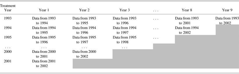
The data set was collected by the UMMC, Kuala Lumpur, from 1992 until 2002 (Hazlina et al., Reference Hazlina, Sameem, NurAishah and Yip2004; Asadi et al., Reference Asadi, Sabah Hasan and Abdul Kareem2014a). As shown in Table 9, the data set was divided into nine subsets based on the interval of survival time: first year, second year, … , ninth year.
The nine subsets of observed data of breast cancer from UMMC based on the interval of survival time

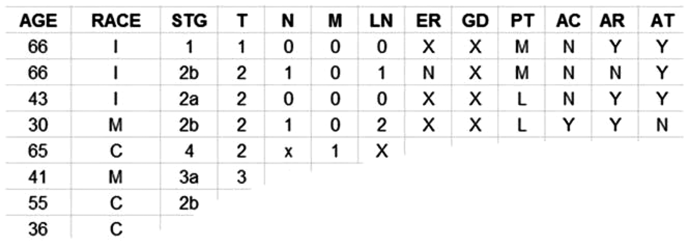
The DSFFNN model was implemented on each data set by considering the class labels. Figure 19 shows the sample of breast cancer data set from the UMMC.
The sample of breast cancer from the University of Malaya Medical Center data set.

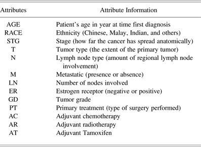
As Table 10 shows, the breast cancer data set contains 13 attributes. The number of input data in the data set is 827, the number of attributes is 13 continuous and 1 attribute for showing the binary class in two cases of alive or dead. The used breast cancer data set from the UMMC has class labels of “0” for alive and “1” for dead as constraints.
The information of the UMMC Breast Cancer data set attributes

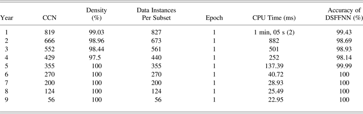
Table 11 shows the results of the implementation of the DSFFNN clustering model on the UMMC breast cancer data set. Table 10 contains of the number of data nodes of each subset; training time per millisecond for each subset during one epoch; and the accuracy of the DSFFNN clustering of each subset of the UMMC breast cancer data set based on the F-measure with 10-folds of the test set.
The results of implementation of the DSFFNN for each subset of the UMMC Breast Cancer data set

Performances of the ESOM and DSOM on the UMMC breast cancer data set are not suitable and efficient; therefore, we compared our results with some methods as reported by Asadi, Asadi, et al. (Reference Asadi, Asadi and Sameem2014). Table 11 shows that the training process of the proposed DSFFNN method for each subset of the UMCC breast cancer data set took one epoch between 22.95 and 1 min, 05 s, and 2 ms of CPU time; the accuracies of the DSFFNN for the breast cancer subdata sets were between 98.14 and 100%. We considered the SOM using BPN as a hybrid method for supervised clustering of each subset (Asadi et al., Reference Asadi, Sabah Hasan and Abdul Kareem2014a). The SOM clustered each subset of the UMMC breast cancer data set after 20 epochs. The BPN model fine-tuned the codebook of weights of unfolding the SOM method instead of random weights. The training process in the BPN was 25 epochs. The results of the hybrid method of the SOM-BPN are shown in Table 12 for every subset. In addition, the principal component analysis (PCA; Jolliffe, Reference Jolliffe1986) was considered as a preprocessing technique for dimension reduction and used by the BPN model (Asadi et al., Reference Asadi, Sabah Hasan and Abdul Kareem2014a). The PCA is a classical multivariate data analysis method that is useful in linear feature extraction and data compression. Table 12 shows the result of the PCA-BPN hybrid model for every subset of the UMMC breast cancer data set. The PCA spent the time of the CPU for dimension reduction of the data, and the BPN used the output of the PCA for classification after several epochs.
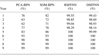
The accuracies of clustering methods on the UMMC Breast Cancer data set

The results of Table 12 show the accuracies of implementation of the PCA-BPN model for the breast cancer data set were between 62% and 99%, and the accuracies of implementation of the SOM-BPN model for each subset of the breast cancer data set were between 71% and 99%. Furthermore, the training process for each subset of the UMMC breast cancer data set by the RSFFNN clustering took one epoch between 13.7 and 43 s of CPU time, and the accuracies of the RSFFNN for these subdata sets were between 98.29% and 100%. Table 12 shows the DSFFNN has desirable results.
4. DISCUSSION AND CONCLUSION
In the online nonstationary data environment such as credit card transactions, the data are often high massive continuous, the distributions of data are not known, and the data distribution may be changed over time. In the real online area, the static UFFNN are not suitable to use; however, they are generally considered as the fundamental clustering methods and are adapted/modified to be used in nonstationary environments, and form the current ODUFFNN clustering methods such as the ESOM and DSOM (Kasabov, Reference Kasabov1998; Schaal & Atkeson, Reference Schaal and Atkeson1998; Bouchachia et al., Reference Bouchachia, Gabrys and Sahel2007; Hebboul et al., Reference Hebboul, Hacini and Hachouf2011). However, the current ODUFFNN clustering methods generally suffer from high training time and low accuracy of clustering, as well as high time and high memory complexities of clustering as scalability of their algorithms (Kasabov, Reference Kasabov1998; Andonie & Kovalerchuk, Reference Andonie and Kovalerchuk2007; Bouchachia et al., Reference Bouchachia, Gabrys and Sahel2007; Rougier & Boniface, Reference Rougier and Boniface2011). Essentially, we recognized the reasons of the problems of the current ODUFFNN clustering methods are the structure and features of the data, such as size and dimensions of data, growing of the number of clusters, and size of the network during clustering; and the topology and algorithm of the current ODUFFNN clustering method, such as using random weights, distance thresholds and parameters for controlling tasks during clustering, and relearning over several epochs, which takes time and clustering is considerably slow. In order to overcome the problems, we developed the DSFFNN clustering model with one epoch training of each online input data. Dynamically, after each entrance of the online input data, the DSFFNN learns and stores important information about the current online data, such as the weights, and completes a code book of the nonrandom weights. Then, a unique and standard weight vector such as the BMW is extracted and updated from the codebook. Consequently, a single-layer DSFFNN calculates the exclusive distance threshold of each online data based on the BMW vector. The online input data are clustered based on the exclusive distance threshold. In order to improve the resulting quality of the clustering, the model assigns a class label to the input data through the training data. The class label of each unlabeled input data is predicted by considering a linear activation function and the exclusive distance threshold. Finally, the number of clusters and the density of each cluster are updated.
To evaluate the performance of the DSFFNN clustering method, we compared the results of the proposed method with the results of other related methods for several data sets from the UCI Repository such as the Arcene data set. In addition, we showed that the DSFFNN method has the capability to be used in different environments, such as the prediction of the hydrate formation temperature, with high accuracy. In this section, we consider a real and original medical data set from the UMMC on the subject of breast cancer. Clustering the medical data sets is difficult because of limited observation, information, diagnosis, and prognosis of the specialist; incomplete medical knowledge; and lack of enough time for diagnosis (Melek & Sadeghian, Reference Melek and Sadeghian2009). However, the proposed DSFFNN method has the capability to overcome some of the problems associated with clustering in the prediction of survival time of the breast cancer patients from the UMMC. Table 13 shows the time and memory complexity of the proposed method and some related clustering methods.
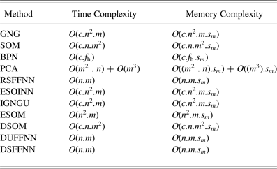
The time complexities and memory complexities of the DSFFNN method and some related methods

The DSFFNN model has time complexity and memory complexity of O(n.m) and O(n.m.s m), respectively. Parameters n, m, and s m are the number of nodes, attributes, and size of each attribute, respectively; in addition, f h is the number of hidden layers and c is the number of iterations. The experimental results showed that the time usage, accuracy, and memory complexity of the proposed DSFFNN clustering method were superior results by comparison with related methods. As shown in Table 14, we compare the DSFFNN clustering method with some strong current ODUFFNN clustering methods.
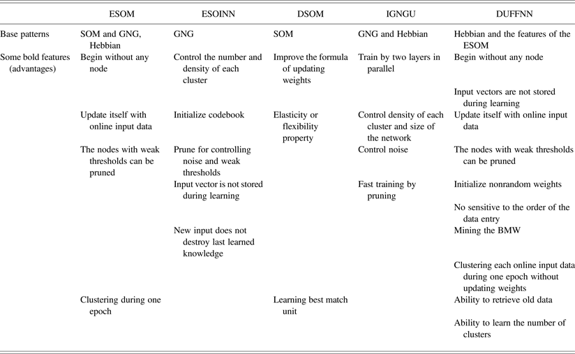
Comparison of the DUFFNN clustering method with some current online dynamic unsupervised feedforward neural network clustering methods

Table 14 shows some FFNN clustering methods such as the SOM and the GNG, which are used as base patterns and improved by the authors for proposing current ODUFFNN clustering methods (Asadi et al., Reference Asadi, Sabah Hasan and Abdul Kareem2014b). As we explained in Section 1, the methods inherited the properties of the base patterns, but by improving their structures; consequently, the ODUFFNN clustering methods obtained new properties. The DSFFNN clustering method inherits the structure, features, and capabilities of the RSFFNN clustering. The DSFFNN clustering with incremental lifelong or online learning property is developed for real nonstationary environments, and it is a flexible method, and with each online continuous data, immediately updates all nodes, weights, and distance thresholds. The proposed DSFFNN method is able to learn the number of clusters, without having any constraint and parameter for controlling the clustering tasks, based on the total thresholds; and it generates the clusters during just one epoch. The DSFFNN is a flexible model, and by changing the BMW, it immediately reclusters the current online data node and old nodes dynamically, and clusters all data nodes based on the new structure of the network without suffering or destroying old data. The DSFFNN clustering method is able to control or delete attributes with weak weights to reduce the data dimensions, and data with solitary thresholds in order to reduce noise.
Future research works may focus to apply the DUFFNN and the DSFFNN clustering method in order to cluster higher dimensional data with the higher number of classes in the big data environment.
Roya Asadi is a PhD candidate researcher in computer science with artificial intelligence (neural networks) at the University of Malaya. She received a bachelor's degree in computer software engineering from Hahid Beheshti University and the Computer Faculty of Data Processing Iran Co. (IBM). Roya obtained a master's of computer science in database systems from UPM University. Her professional working experience includes 12 years of service as a Senior Planning Expert 1. Roya's interests are in data mining, artificial intelligence, neural network modeling, intelligent multiagent systems, system designing and analyzing, medical informatics, and medical image processing.
Sameem Abdul Kareem is an Associate Professor in the Department of Artificial Intelligence at the University of Malaya. She received a BS in mathematics from the University of Malaya, an MS in computing from the University of Wales, and a PhD in computer science from University of Malaya. Dr. Kareem's interests include medical informatics, information retrieval, data mining, and intelligent techniques. She has published over 80 journal and conference papers.
Shokoofeh Asadi received a bachelor's degree in English language translation (international communications engineering) from Islamic Azad University and a master's degree in agricultural management engineering from the University of Science and Research. Her interests are English language translation, biological and agrcultural engineering, management and leadership, strategic management, and operations management.
Mitra Asadi is a Senior Expert Researcher at the Blood Transfusion Research Center in the High Institute for Research and Education in Transfusion Medicine. She received her bachelor's degree in laboratory sciences from Tabriz University and her English language translation degree and master's of English language teaching from Islamic Azad University. She is pursuing her PhD in entrepreneurship technology at Islamic Azad University of Ghazvi.