3.1. Background flow

The RM instability flow is a combination of two types of motion: the background motion, which causes the entire interface to move downwards, and the local rotational motion, which causes the interface amplitude to increase over time (Stanic et al. Reference Stanic, Stellingwerf, Cassibry and AbarzhiS2012; Dell et al. Reference Dell, Pandian, Bhowmick, Swisher, Stanic, Stellingwerf and Abarzhi2017; Zhang et al. Reference Zhang, Zhao, Ding and Luo2023c ). The former is determined by the shock intensity and fluid properties (e.g. density and specific heat ratio), which exists in both perturbed and unperturbed cases. The latter quantifies the degree of instability, which occurs only in the case of a perturbed interface. In most circumstances, such as planar RM instability, the former is uniform and does not influence the latter, allowing the two motions to be decoupled. However, for the convergent RM instability, the background flow is time-dependent, which induces RT stability or instability, significantly affecting the instability growth. Therefore, obtaining the background motion is crucial for fully understanding and predicting the convergent RM instability. Since there is currently no analytical solution for such a background flow, a quasi-one-dimensional (1-D) experiment corresponding to an unperturbed cylindrical SF $_6$ layer surrounded by air subjected to a cylindrically convergent shock is first conducted.

Figure 2.

$(a)$ Schlieren images showing the evolution of an unperturbed $\text {SF}_6$ layer accelerated by a cylindrical convergent shock. $(b)$ Sketches of the waves and interfaces at corresponding moments. The white dotted lines indicate the thin filaments used to form the initial interfaces. The unit of numbers is $\unicode {x03BC}$ s. ICS, the incident cylindrical shock; $\text {II}_i$ , the initial interface ( $i = 1, 2$ refers to the outer and inner interfaces, respectively); $\text {SI}_i$ , the shocked interface; $\text {TS}_i$ , the transmitted shock; RS, the reflected shock; RW, the rarefaction wave.

Representative schlieren images illustrating the motions of the interfaces and waves for the unperturbed case are displayed in figure 2 $(a)$ . To better illustrate the motion of the gas layer, sketches of the waves and interfaces at corresponding moments are provided in figure 2 $(b)$ . The time origin in this work is defined as the moment at which the incident shock arrives at the mean position of the outer interface. At the beginning (-20 $\unicode {x03BC}$ s), both the outer (II $_1$ ) and inner (II $_2$ ) interfaces, along with the incident convergent shock (ICS), are clearly discerned. This demonstrates the feasibility and reliability of the current experimental methods. As time goes on, the ICS propagates downstream and impinges upon the outer air/SF $_6$ interface, bifurcating immediately into an ingoing transmitted shock ( $\text {TS}_1$ ) and an outgoing reflected shock (RS) (39 $\unicode {x03BC}$ s). After that, the shocked outer interface starts moving and gradually leaves its original position. Later, the $\text {TS}_1$ collides with the inner interface, splitting into a second transmitted shock ( $\text {TS}_2$ ) and an outgoing rarefaction wave (RW) (119 $\unicode {x03BC}$ s). The shocked inner interface moves downstream following the $\text {TS}_2$ . Later, the outgoing RW stretches and accelerates the outer interface, while simultaneously generating an ingoing compression wave within the layer (not visible in schlieren images due to its weak intensity). As expected, no reflected shock is observed here since the convergent shock tube has an open outlet. The white dotted lines in figure 2 $(a)$ indicate the locations of the protruding filaments (i.e. the locations of initial interfaces). It should be noted that the shock impact can cause the soap film to atomise into small droplets. According to Cohen (Reference Cohen1991) and Ranjan et al. (Reference Ranjan, Niederhaus, Oakley, Anderson, Bonazza and Greenough2008), the mean radius of soap droplets in the present experiment is estimated to be approximately 30 $\unicode {x03BC}$ m for $M\sim$ 1.3. These droplets are negligibly small compared with the characteristic length scales of the flow and thus have a negligible influence on interface dynamics. This conclusion has been thoroughly validated in our previous work. For instance, previous numerical simulations of shock–bubble interactions that excluded soap droplets showed excellent agreement with experimental results in terms of both interface morphology and growth rate (Ding et al. Reference Ding, Si, Chen, Zhai, Lu and Luo2017a ). Furthermore, shock-tube experiments on RM instability at single-mode interfaces, generated using the soap film technique, exhibited linear growth rates consistent with impulsive model predictions that ignore soap droplets (Liu et al. Reference Liu, Liang, Ding, Liu and Luo2018). The consistency across experiments (with soap droplets), simulations and theories (without soap droplets) confirms that the influence of soap droplets on interface evolution is negligible. Also, the influence of boundary layer on the flow is negligible during the time of interest (Luo et al. Reference Luo, Li, Ding, Zhai and Si2019; Zhang et al. Reference Zhang, Ding, Si and Luo2023b ).

Figure 3.

$(a)$ Trajectories of the interfaces and waves. $(b)$ Time derivatives of the interface displacement. The abbreviations are the same as those in figure 2.

An $R{-}t$ diagram depicting the trajectories of the waves and interfaces is plotted in figure 3 $(a)$ , which reflects the time-dependence of the flow field. The time derivative of the interface displacement is also given in figure 3 $(b)$ . Slight fluctuations are observed in the calculated interface velocity, which is primarily due to the limited temporal resolution of the schlieren images. Accelerated by the incident convergent shock, the outer interface attains an initial velocity of 101.1 m s⁻¹. Subsequently, it is accelerated to 124.0 m s⁻¹ by the RW. After the impact of the first transmitted shock TS $_1$ , the inner interface moves inwards at a velocity of 117.7 m s⁻¹. As the waves move away, both the inner and outer interfaces present uniform motion, with only slight deceleration at the later stage. It indicates that the RT effect is significantly mitigated in the current shock tube. Considering the measurement error, both interfaces can be regarded as moving uniformly throughout the entire experimental duration. The extended period of uniform motion for the inner and outer interfaces provides a rare opportunity to analyse the effects of nonlinearity and interface coupling on convergent RM instability, which will be discussed in § 3.2. Despite this, we emphasise that the base flow in our configuration is complex, characterised by a non-uniform pressure field behind the incident shock and an expansion-shock structure resulting from shock–interface interactions. This generates a spatially and temporally varying pressure field, which serves as the background flow for perturbation growth. Such a background flow is particularly crucial as it can significantly influence instability development through several mechanisms. First, the non-uniform pressure field behind the incident shock directly modulates baroclinic vorticity generation, the primary driving mechanism of the RM instability. Second, the expansion-shock structure introduces additional wave–interface interactions, altering perturbation growth rates through multiple reflection and transmission events. Third, the time-dependent nature of the flow field introduces additional effects that are absent in conventional planar configurations. These characteristics of the base flow are essential for understanding interface dynamics and thus are carefully incorporated into the vortex method (§ 4).

Although a gas concentration detector is used to measure the oxygen concentration in the gas mixture exhausted from the outflow hole, it ensures only a high concentration of $\text {SF}_6$ inside the layer rather than directly measuring the mass fraction of $\text {SF}_6$ . In this work, the mass fraction of $\text {SF}_6$ is estimated using the following method. In a 1-D flow where a shock impacts a light/heavy interface, the resulting flow typically consists of four uniform regions separated by a reflected shock, a transmitted shock and the interface itself. When a cylindrical convergent shock has just passed across an unperturbed cylindrical interface, the flow can be approximated as 1-D along the radial direction. According to 1-D gas dynamics theory, we can establish relations between the flow parameters on either side of the reflected and transmitted shocks. Also, a compatibility relation exists (i.e. continuity of normal velocity and pressure) across the interface. With these relations, the following equation can be derived:

(3.1) \begin{equation} \left [\frac {\left (\Lambda _2-1\right ) \rho _1}{\left (\Lambda _1-1\right ) \rho _2}\right ]^{1 / 2} \frac {P_t-1}{\left (P_t \Lambda _2+1\right )^{1 / 2}}=\frac {P_i-1}{\left (P_i \Lambda _1+1\right )^{1 / 2}}-\left (\frac {\rho _1}{\rho _1^{\prime }}\right )^{1 / 2} \frac {P_t-P_i}{\left (P_t \Lambda _1+P_i\right )^{1 / 2}}, \end{equation}

where

(3.2) \begin{equation} \left .\begin{array}{c} \Lambda _1=(\zeta _1+1)/(\zeta _1-1)\\[2 mm] \Lambda _2=(\zeta _2+1)/(\zeta _2-1)\\[2 mm] P_i=1+2\zeta _1/(\zeta _1+1)\left (M_i^2-1\right )\\[2 mm] \rho _1/\rho _1^{\prime }=\left[\left(\zeta _1-1\right) M_i^2+2\right]/\left[\left(\zeta _1+1\right) M_i^2\right] \end{array}\right \rbrace . \end{equation}

Here, $\zeta _1$ and $\rho _1$ are the specific heat ratio and density outside the layer, respectively, $\zeta _2$ and $\rho _2$ are the specific heat ratio and density inside the layer, respectively, $P_i$ ( $P_t$ ) refers to the pressure ratio across the incident shock (transmitted shock) and $\rho _i^{\prime }$ to the fluid density behind the incident shock. In experiment, the velocity of the incident shock propagating in pure air is measured to be 445.0 m s $^{-1}$ , corresponding to $M_i$ = 1.27. Based on the measured velocities of the incident and transmitted shocks, the mass fraction of SF $_6$ can be determined through an iterative method. Specifying an arbitrary initial value between 0 and 1 for the mass fraction of SF $_6$ inside the layer, the flow parameters inside the layer (e.g. $\rho _2$ and $\zeta _2$ ) can be obtained. Substituting these known parameters into (3.1), the pressure ratio across the transmitted shock ( $P_t$ ) can be solved, namely, the strength of the transmitted shock is available. If the Mach number of the transmitted shock obtained is higher than the measured one, the value of mass fraction is slightly reduced; otherwise, it is increased. This process is repeated multiple times until the calculated value is in good agreement with the measured one (i.e. their difference is less than 0.1 %). For the unperturbed case here, the mass fraction of SF $_6$ is calculated to be 92.5 %. Using this value, the flow velocity behind the transmitted shock is calculated to be 99.2 m s⁻¹ based on 1-D gas dynamics theory. This result is in good agreement with the measured value (101.1 $\pm$ 2.0 m s⁻¹), indicating the reliability of the concentration calculation method.

3.2. Evolution of perturbed layer

Eight types of perturbed $\text {SF}_6$ layers with various thicknesses and shapes, subjected to a cylindrical convergent shock, are then examined. Specifically, two layer thicknesses are considered: the outer interface is fixed at $R_{1\_0}$ = 280 mm, while the inner interface takes radii of $R_{2\_0}$ = 260 mm and 240 mm, corresponding to the layer thicknesses of $d_0$ = 20 mm and 40 mm, respectively. For each thickness, various shapes of the inner and outer interfaces are considered: unperturbed outer interface and sinusoidal inner interface (case US); sinusoidal outer interface and unperturbed inner interface (case SU); sinusoidal outer and inner interfaces with in-phase perturbations (case IP); and sinusoidal outer and inner interfaces with anti-phase perturbations (case AP). For ease of reference, we designate a gas layer as case d20/d40-SU/US/IP/AP, where the first symbol represents the layer thickness and the second denotes the layer shape. For example, case d20-SU refers to a 20 mm thick layer with a sinusoidal outer interface and an unperturbed inner interface. In this work, interface perturbations with an azimuthal mode number of $n=24$ and an initial amplitude of $a=3$ mm are adopted. These parameters are carefully chosen to enable clear observation of both linear and nonlinear growth stages within our experimental window while maintaining high measurement precision. Specifically, the selection of these parameters is based on several considerations. First, the mode number $n=24$ ensures the observation of multiple wavelengths within our field of view, which is essential for obtaining statistically reliable amplitude measurements. Second, the initial amplitude $a=3$ mm is chosen to be sufficiently small relative to the wavelength to allow observation of the linear stage, yet large enough to ensure accurate measurements and to reach the nonlinear stage within the experimental time frame. While a systematic study of different initial amplitudes and frequencies would be valuable, it lies beyond the scope of the current work, which primarily focuses on elucidating the effects of interface coupling and reverberating waves on instability growth. Detailed parameters corresponding to the initial conditions for each case are listed in table 1, where the Atwood number is defined as $A = (\rho _2-\rho _1)/(\rho _2+\rho _1)$ . 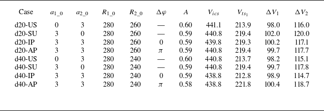The parameters, such as shock strength, gas concentration and interface positions, are nearly identical across these cases, indicating that the background flow remains consistent.

Table 1.

Detailed parameters corresponding to initial conditions for each case. $R_{1\_0}$ ( $R_{2\_0}$ ) is the initial radius of the outer (inner) interface; $a_{1\_0}$ ( $a_{2\_0}$ ) is the initial amplitude of the outer (inner) interface; $\unicode{x0394} \varphi$ is the phase difference between the initial perturbations at the outer and inner interfaces; $A=(\rho _2-\rho _1)/(\rho _2+\rho _1)$ is the Atwood number; $V_{ics}$ is the velocity of the incident cylindrical shock; $V_{ts_1}$ is the velocity of the transmitted shock; $\unicode{x0394} V_1$ ( $\unicode{x0394} V_2$ ) is the post-shock velocity of the outer (inner) interface. The radius and amplitude are in mm and the velocity is in m s⁻¹.

Figure 4.

Schlieren images showing the developments of wave patterns and interfacial morphologies for all cases. The white dotted lines indicate the thin filaments used to form the soap film interfaces. The symbols are the same as those in figure 2. The unit of numbers is $\unicode {x03BC} \mathrm{s}$ .

3.2.1. Schlieren results

Developments of the interface morphologies and wave patterns, illustrated by sequences of schlieren images, are presented in figure 4. Here, we take case d40-US as an example to detail the evolution process. At the beginning (−18 $\unicode {x03BC}$ s), an incident convergent shock ICS, along with an unperturbed outer interface II $_1$ and a sinusoidal inner interface II $_2$ , is clearly observed. The velocity of the incident shock is measured to be 441.1 m s⁻¹ just before its collision with the outer interface, corresponding to Mach number $M_i$ = 1.27. After the incident shock passes across the outer interface, it bifurcates into an upstream-moving reflected shock RS and a downstream-moving transmitted shock TS $_1$ . The shocked outer interface SI $_1$ moves downstream with an initial velocity of approximately 98.2 m s⁻¹. During this process, it maintains a perfectly cylindrical shape with no instability due to the complete alignment between the incident shock and the initial interface. Afterwards, the cylindrical transmitted shock TS $_1$ collides with the sinusoidal inner interface, immediately bifurcating into a second transmitted shock TS $_2$ and an outgoing rarefaction wave RW (281 $\unicode {x03BC}$ s). Differing from the unperturbed case, both the TS $_2$ and RW here exhibit a sine-like perturbation. Particularly, the RW has the same perturbation phase as the sinusoidal inner interface, while TS $_2$ presents an opposite phase. After the impact of TS $_1$ , the amplitude of the inner interface experiences a sudden drop due to shock compression, then reduces gradually to zero (i.e. phase inversion) and finally increases persistently with an opposite phase. Despite the rapid deformation of the inner interface, the outer interface presents no instability during the entire experimental period (741 $\unicode {x03BC}$ s). This phenomenon is also seen in case d40-SU, where the outer interface exhibits a large perturbation amplitude at 733 $\unicode {x03BC}$ s, while the inner interface remains perfectly cylindrical. Previous studies have shown that, at late stages when the waves move away from the gas layer, the compressibility effect becomes negligible and interface coupling dominates the instability growth (Mikaelian Reference Mikaelian1995, Reference Mikaelian2005; Liang & Luo Reference Liang and Luo2021). The decoupling of the inner and outer interfaces observed here indicates that the interface coupling effect is sufficiently weak for 40 mm thick layers.

As the layer thickness is reduced to 20 mm (e.g. case d20-US), the outer interface also presents no instability growth at the early stage. Later, the disturbed RW stretches and accelerates the outer interface, seeding a slight perturbation on it. As time proceeds, this small perturbation grows continuously with time. At late stages (714 $\unicode {x03BC}$ s), the outer interface exhibits a considerably large perturbation that is in phase with the perturbed inner interface. Similarly, in case d20-SU, the initially unperturbed inner interface presents a large perturbation that is in phase with the perturbed outer interface (724 $\unicode {x03BC}$ s). The present results manifest that interface coupling plays a significant role in the evolution of 20 mm thick layers. For case d20-AP, after the shock impact, the amplitude of the inner interface first suffers a gradual reduction to zero (i.e. phase inversion), then increases persistently with the same phase as the outer interface. In contrast, in case d20-IP, the deformed inner interface exhibits an opposite phase relative to the outer interface at late stages. According to the analysis of Mikaelian (Reference Mikaelian2005), for two sinusoidal interfaces that have the same phase (opposite phases), interface coupling promotes (suppresses) the perturbation growth at either interface. This reasonably explains why the perturbation growth at either interface in case d20-AP is much quicker than that in case d20-IP. The present experimental results demonstrate that the phase difference between the two interfaces determines the interface coupling effect and further affects the instability growth rate at each interface. To more clearly reveal the effect of phase difference between the two interfaces on the layer evolution, contours of waves and interfaces at typical moments for the 20 mm thick layers with various shapes are depicted in figure 5. It should be emphasised that this is the first long-term observation of convergent RM instability in a gas layer. Although the observed phenomena qualitatively align with the RM instability triggered by planar shocks (Liang & Luo Reference Liang and Luo2021) or divergent shocks (Zhang et al. Reference Zhang, Ding, Li, Zou and Luo2023a ), the experimental data offer a rare opportunity to analyse the regimes of convergent RM instability.

Figure 5.

Sketches of the wave patterns and interface morphologies at typical moments for 20 mm thick layers. The symbols are the same as those in figure 2.

3.2.2. Growth of perturbation amplitude

Under the incompressible, inviscid and irrotational flow assumption, Wang et al. (Reference Wang, Wu, Guo, Ye, Liu, Zhang and He2015) has derived a weakly nonlinear model for the cylindrical RM instability at an isolated single-mode interface. A brief description of this model is given below. A velocity potential is first introduced for either fluid across the interface, which satisfies the Laplace equation. By applying the kinematic and dynamic boundary conditions (i.e. normal velocities of both fluids match and also pressure is continuous across the interface), three additional equations for the velocity potentials are derived. By expanding the perturbation displacement and velocity potentials into a power series, the first-, second- and third-order governing equations, each expressed as a second-order ordinary differential equation, can be obtained. It is important to note that obtaining a general solution for the perturbation growth at a cylindrical interface with an arbitrary implosion or explosion history is highly challenging. By assuming uniform motion of the interface, this problem becomes significantly simpler and a third-order analytical solution can be derived. For more details about the model, readers are referred to the original work (Wang et al. Reference Wang, Wu, Guo, Ye, Liu, Zhang and He2015).

Figure 6.

Comparison of the amplitude growths of the (a,c) outer and (b,d) inner interface between experiments and the prediction of Wang et al. (Reference Wang, Wu, Guo, Ye, Liu, Zhang and He2015).

Temporal variations of the amplitudes of the inner and outer interfaces for all perturbed layers are plotted in figure 6, with the predictions from Wang et al. (Reference Wang, Wu, Guo, Ye, Liu, Zhang and He2015) provided for comparison. The amplitude is defined as half the total width of the interface, i.e. half the maximum distance between the spike head and the bubble tip. Note the parameters required by Wang et al. (Reference Wang, Wu, Guo, Ye, Liu, Zhang and He2015), such as the initial growth rate, interface displacement, velocity and acceleration, are measured from experiment. We first discuss the instability growth at the outer interface. As seen in figures 6(a) and 6(c), for either thickness, the perturbation growths at the outer interface for the SU, IP and AP cases collapse quite well before the arrival of RW, which indicates a negligible interface coupling effect during the early stage. This can be interpreted from the perspective of pressure disturbances. In compressible fluids, perturbations at one interface propagate to another interface via pressure disturbances, which travel at the speed of sound. It means that these disturbances cannot cross through reverberating waves (such as RW) to influence the other interface. Thus, before the arrival of RW, the evolution of the outer interface suffers no influence of the inner interface and vice versa. This also explains why the weakly nonlinear model of Wang et al. (Reference Wang, Wu, Guo, Ye, Liu, Zhang and He2015), developed for cylindrical RM instability at a single interface, provides a good prediction of instability growth before the arrival of RW for all cases. Later, the RW stretches and accelerates the outer interface, notably enhancing the instability growth except in case d20-IP (the reason is explained later). For a thick layer, the effect of RW is weakly dependent on the interface shape, as indicated by figure 6(a). It is seen that the RW significantly enhances the perturbation growth in case d40-AP, moderately in case d40-SU and minimally in case d40-IP. This can be explained by the wave patterns in figure 5, where the perturbed RW is out of phase with the deforming outer interface for the AP layer, producing more baroclinic vorticity, whereas it is in phase with the deforming outer interface for the IP layer, producing less baroclinic vorticity. Since the RW is weak in the present experiment, the difference in the instability growth among the three cases is small. At late stages, the amplitude of the outer interface remains consistent across all 40 mm thick layers, indicating a negligible interface coupling effect. This is confirmed by schlieren results, where the outer interface presents nearly the same perturbation at late stages across cases d40-AP, d40-IP and d40-SU.

For a thin layer, interface coupling becomes pronounced, and the instability growth is influenced by both the RW and interface coupling. For case d20-AP, the RW is out of phase with the outer interface (see figure 5), significantly enhancing the perturbation growth. Also, the interface coupling effect further promotes the instability growth in this case. As a result, this scenario exhibits the fastest instability growth following the RW impact. In case d20-IP, the RW is in phase with the outer interface, leading to only a modest increase in instability growth. Nevertheless, the interface coupling inhibits instability growth in this case. As a consequence, after the RW impact, the perturbation growth at the outer interface is slower compared with an isolated interface. It indicates that the influence of interface coupling outweighs the effect of RW. In case d20-SU, the effects of RW and interface coupling are moderate, resulting in a moderate growth rate that is slightly higher than that of an isolated interface. The present results show that both the effect of RW and interface coupling are highly sensitive to layer shape. Compared with the effect of RW, interface coupling plays a more significant role in instability growth, particularly at later stages.

Then, we examine the instability growth at the inner interface. As shown in figure 6(b), for thick layers, the instability growth at the inner interface remains consistent across the IP, AP and US cases. Given the initial growth rate measured from experiment, the model of Wang et al. (Reference Wang, Wu, Guo, Ye, Liu, Zhang and He2015), which ignores the effect of rippled shock, gives a reasonable prediction of the instability growth throughout the entire experimental duration. This indicates that for thick layers, the effects of waves and interface coupling are negligibly weak, allowing the inner interface to evolve independently as if it were isolated. In contrast, for thin layers, notable discrepancy is observed among the IP, AP and US cases from the very beginning. Specifically, the AP case exhibits the largest initial growth rate (prior to phase inversion), the US case shows a moderate growth rate and the IP case has the smallest growth rate. This indicates that the effect of rippled TS $_1$ on the inner interface is significant and must be considered, which will be detailed in § 4. After phase inversion, the AP case continues to show the highest growth rate, the US case maintains a moderate rate and the IP case shows the smallest rate. This is attributed to the interface coupling effect: it significantly promotes instability growth in the d20-AP case, moderately promotes instability growth in the d20-SU case and suppresses instability growth in the d20-IP case. The model of Wang et al. (Reference Wang, Wu, Guo, Ye, Liu, Zhang and He2015) fails to predict the perturbation growth at late stages, despite initially matching the experimental results. The discrepancy is primarily due to the neglect of interface coupling in the model of Wang et al. (Reference Wang, Wu, Guo, Ye, Liu, Zhang and He2015). The underlying regimes driving the diverse perturbation growth behaviours observed here are explored in § 4.

4.1. Considering the background flow

In contrast to the RT and KH instabilities, in the context of RM instability, each fluid element at the interface not only experiences local rotational motion, but also acquires a background velocity due to the shock impact. Especially, the convergent RM instability involves an unsteady, non-uniform background flow, which could significantly influence the transport of vortex sheet strength. Therefore, accurately estimating the effect of background flow on the vortex sheet transport is crucial for the vortex method. For this purpose, the velocity on either side of the interface is decomposed into two components:

(4.1) \begin{equation} \boldsymbol {u}_i = {\boldsymbol {u}}_{i}^{\prime } + {\boldsymbol {u}_\infty }, \end{equation}

where $\boldsymbol {u}_{i}^{\prime }$ is the shear velocity, which is discontinuous across the interface, and $\boldsymbol {u}_\infty$ is the background velocity, which remains invariant across the interface. Thus, the vortex sheet strength can be expressed as

(4.2) \begin{equation} \gamma =({{\boldsymbol {u}}_1} - {{\boldsymbol {u}}_2}) \cdot {\boldsymbol {s}}=({{\boldsymbol {u}}_1^{\prime }} - {{\boldsymbol {u}}_2^{\prime }}) \cdot {\boldsymbol {s}}. \end{equation}

Also, the Lagrange velocity of the interface can be written as

(4.3) \begin{equation} \boldsymbol {U}=(\boldsymbol {u}_1+\boldsymbol {u}_2)/2=\boldsymbol {U^{\prime }}+\boldsymbol {u}_\infty , \end{equation}

where $\boldsymbol {U^{\prime }}=(\boldsymbol {u}_1^{\prime }+\boldsymbol {u}_2^{\prime })/2$ denotes the average of the shear velocities on either side of the interface. Substituting (4.2) and (4.3) into the governing equation of the original vortex method (A6), an extended transport equation for the vortex sheet strength accounting for the background flow is obtained:

(4.4) \begin{align} \dfrac {{{\rm d}\gamma }}{{{\rm d}t}} +\gamma \left(\dfrac {{\partial {\boldsymbol {U^{\prime }}}}}{{\partial s}}+\dfrac {{\partial {\boldsymbol {u}_\infty }}}{{\partial s}} \right)\cdot {\boldsymbol {s}} =&\; 2A \left[ \left(\dfrac {{{\rm d}{\boldsymbol {U^{\prime }}}}}{{{\rm d}t}} + \dfrac {{{\rm d}{\boldsymbol {u}_\infty }}}{{dt}}\right) \cdot {\boldsymbol {s}}+ \dfrac {1}{8}\dfrac {{\partial {\gamma ^2}}}{{\partial s}}\right] + 2A\boldsymbol {g}\cdot \boldsymbol {s} \nonumber\\ & -\frac {2}{\rho _1+\rho _2} \frac {\partial \left (p_1-p_2\right )}{\partial s}, \end{align}

where

(4.5) \begin{equation} \begin{aligned} & \dfrac {d{\boldsymbol {U}^{\prime }}}{{dt}}=\dfrac {{\partial {\boldsymbol {U}^{\prime }}}}{{\partial t}}+\left(\boldsymbol {U}^{\prime }+\boldsymbol {u}_\infty \right)\cdot \nabla \boldsymbol {U}^{\prime }; \ \ \ \ \ & \dfrac {d{\boldsymbol {u}_\infty }}{{dt}}=\dfrac {{\partial {\boldsymbol {u}_\infty }}}{{\partial t}}+\left(\boldsymbol {U}^{\prime }+\boldsymbol {u}_\infty \right)\cdot \nabla \boldsymbol {u}_\infty . \end{aligned} \end{equation}

Equation (4.4) is referred to as the vortex-b model in this work.

The term ${\partial {\boldsymbol {u}_\infty }}/{\partial s}$ on the left-hand side of (4.4) represents the stretching of the vortex sheet caused by non-uniform background flow. The term ${{\rm d}{\boldsymbol {u}_\infty }}/{{\rm d}t}$ on the right-hand side of (4.4) represents the generation/elimination of vorticity caused by unsteady background flow. In the context of RT and KH instabilities, the background velocity is typically zero, i.e. $\boldsymbol {u}_\infty =0$ . For this situation, (4.4) reduces to the original vortex sheet model represented by (A6). For the planar RM instability, the background velocity is constant (i.e. ${{\rm d}{\boldsymbol {u}_\infty }}/{{\rm d}t}=0$ and ${\partial {\boldsymbol {u}_\infty }}/{\partial s}=0$ ), and (4.4) also reduces to (A6). It indicates that the background flow in planar RM instability produces no effect on the vortex transport and can be ignored. However, for the convergent RM instability, the background velocity is unsteady in time ( ${{\rm d}{\boldsymbol {u}_\infty }}/{{\rm d}t}\neq 0$ ) and also non-uniform in space ( ${\partial {\boldsymbol {u}_\infty }}/{\partial s}\neq 0$ ), significantly affecting the transport of vortex sheet strength. This is a unique characteristic of convergent RM instability, as has been demonstrated in experiment (Ding et al. Reference Ding, Si, Yang, Lu, Zhai and Luo2017b ). Considering there is no analytical solution for the background flow of convergent RM instability, in this work, $\boldsymbol {u}_\infty$ is obtained by fitting the interface position measured from experiment. Note in the present experiments, the surface tension of the soap film interface is negligibly small and also the effect of gravitational acceleration on the interface evolution is negligible. Thus, the last two terms on the right-hand side of (4.4) can be ignored.

Given the position and strength of a vortex sheet, the shear-induced velocity of any fluid point at the vortex sheet, $\boldsymbol {U'}$ , can be calculated according to the Birkhoff–Rott equation:

(4.6) \begin{equation} {u}-i{v}=\frac {i}{2 \lambda } \int _0^\lambda \gamma ' \cot \frac {\pi (z-{z}')}{\lambda } {\rm d} {s}'. \end{equation}

Here, $u$ and $v$ represent the horizontal and vertical components of the shear-induced velocity $\boldsymbol {U'}$ , $\lambda$ is the wavelength, $\boldsymbol {z}=x+\mathrm {i} y$ in complex notation, and ${\gamma }'=\gamma ({s}'), \boldsymbol {z}=\boldsymbol {z}(s), {\boldsymbol {z'}}=\boldsymbol {z}({s}')$ .

As we know, either the KH, RT or RM instability could develop into a roll-up at the late nonlinear stage, which corresponds to the formation of singularities in the vortex method. To avoid the formation of singularities, a desingularisation parameter, $\delta$ , originally proposed by Krasny (1986), is applied to (4.6). Then, the velocity of each fluid point at the vortex sheet is calculated by

(4.7) \begin{equation} {\begin{array}{c} u =\dfrac {1}{2 \lambda } \int _{0}^{\lambda } \dfrac {\sinh (k y-k y^{\prime } )}{\cosh \left (k y-k y^{\prime }\right )-\cos \left (k x-k x^{\prime }\right )+\delta ^2} \gamma ^{\prime } d s^{\prime }, \\[12pt] v =-\dfrac {1}{2 \lambda } \int _{0}^{\lambda }\dfrac {\sin (k x-k x^{\prime } )}{\cosh \left (k y-k y^{\prime }\right )-\cos \left (k x-k x^{\prime }\right )+\delta ^2} \gamma ^{\prime } {\rm d} s^{\prime }. \end{array}} \end{equation}

In this work, $\delta =0.01$ is adopted. The interface position is governed by

(4.8) \begin{equation} {\rm d}\boldsymbol {z}/{\rm d}t=\boldsymbol {U'}+\boldsymbol {u}_\infty . \end{equation}

Given the initial distribution of vortex sheet strength, temporal evolution of the vortex sheet can be obtained by numerically solving (4.4), (4.7) and (4.8). During this process, the vortex sheet is usually discretised into several hundred to a thousand Lagrangian points. Time integration is performed using an iteration method following Sohn et al. (Reference Sohn, Yoon and Hwang2010). A convergence study indicates that $\unicode{x0394} t=0.5$ $\unicode {x03BC}$ s provides sufficient accuracy for our results and is therefore selected as the time step for all calculations in this work.

4.2. Estimating the initial vortex sheet strength

For the RT and KH instabilities, the initial vortex sheet strength can be readily specified (Sohn et al. Reference Sohn, Yoon and Hwang2010; Sohn Reference Sohn2011). In contrast, for the RM instability, the initial vortex sheet strength is influenced by the dynamic interaction between the incident shock and the material interface. This interaction in compressible flow complicates the estimation of vortex sheet strength significantly. For a planar shock interacting with a perturbed interface, a scaling law that clearly reveals the vortex sheet strength along the interface has been derived based on shock dynamics theory (Samtaney & Zabusky Reference Samtaney and Zabusky1994; Samtaney et al. Reference Samtaney, Ray and Zabusky1998). It is formulated as

(4.9) \begin{equation} \gamma (s)=\frac {{\rm d}\Gamma }{{\rm d}s}=\frac {2c_0}{\zeta +1}\left(1-\frac {1}{\sqrt {\eta }}\right)\big(1+M^{-1}+2M^{-2}\big)(M-1)\sin \alpha \end{equation}

for a light/heavy interface, and

(4.10) \begin{equation} \gamma (s)=\frac {{\rm d}\Gamma }{{\rm d}s}=\frac {4c_0}{\zeta +1}\left(1-\frac {1}{\sqrt {\eta }}\right)\frac {M^2-1}{1+\frac {2\zeta }{\zeta +1}\left(M^2-1\right)}\sin \alpha \end{equation}

for a heavy/light interface. Here, M is the shock Mach number, $\eta$ the density ratio across the interface, $c_0$ the sound speed of the pre-shock fluid, $\zeta$ the specific heat ratio of the gas, and $\alpha$ the angle between the shock and interface. The above equations account for the variation in the angle between the shock and the interface during the dynamic process of shock–interface interaction. In convergent RM instability, in addition to the variation in the angle between the shock and interface, the shock strength also varies continuously during the shock–interface interaction process. Moreover, for the convergent RM instability at a perturbed gas layer, the inner interface may be impacted by a distorted transmitted shock, for which the shock strength is non-uniform along its surface. Estimating the initial vorticity distribution along an interface impacted by such a distorted convergent shock is challenging.

In this work, we consider a general convergent RM instability, i.e. a sinusoidally distorted shock interacts with a single-mode interface in cylindrical geometry. Considering that the shock–interface interaction occurs within a very short period of time, the shock Mach number is assumed to remain constant during this process. With this assumption, the vortex sheet strength at the fluid point ( $r$ , $\theta$ ) on the interface can be calculated as

(4.11) \begin{align} \gamma (\theta )= \frac {{\rm d}\Gamma }{{\rm d}\theta }(\theta )=\frac {2c_0}{\zeta +1}\left(1-\frac {1}{\sqrt {\eta }}\right)\big(1+M^{-1}(\theta) \big) +2M^{-2}(\theta)(M(\theta )-1)\sin \alpha _1(\theta ) \end{align}

for a fast/slow interface, and

(4.12) \begin{align} \gamma (\theta )= \frac {{\rm d}\Gamma }{{\rm d}\theta }(\theta )=\frac {4c_0}{\zeta +1}\left(1-\frac {1}{\sqrt {\eta }}\right)\frac {M^2(\theta )-1}{1+\frac {2\zeta }{\zeta +1}\big(M^2(\theta \big)-1)} \sin \alpha _2(\theta )\end{align}

for a slow/fast interface. Here,

(4.13) \begin{equation} \begin{array}{c} {\sin {\alpha _{i}(\theta )} = \dfrac {{\left ( {a_{i\_0}^ + {r_{s\_i}} - {a_{s\_i}}r^+_i} \right )n\sin (n\theta )}}{{\sqrt {{r_{s\_i}}^2 + {{\left ( {n{a_{s\_i}}\sin (n\theta )} \right )}^2}} }}} .\end{array} \end{equation}

Here, $r_{s\_i}=R_{s\_i}+a_{s\_i}\cos (n \theta )$ is the shock position with $R_{s\_i}$ being the average radius of shock and $a_{s\_i}$ being the perturbation amplitude of the shock, $a_{i\_0}^ +$ is the initial amplitude of the shocked interface, and $r^+_i=R^+_i+a_{i\_0}^ +\cos (n\theta )$ is the initial radius of the shocked interface. For more details on the derivation process, readers are referred to the original work (Li et al. Reference Li, Ding, Luo and Zou2022). Note that the post-shock amplitude is adopted in the above equations due to shock compression.

Comparison of the instability growth at an isolated single-mode interface among the experiment, the prediction of Wang et al. (Reference Wang, Wu, Guo, Ye, Liu, Zhang and He2015) and the current vortex method is shown in figure 7. It is found in § 3.2 that for thick layers ( $d=$ 40 mm), the evolutions of the inner and outer interfaces are nearly decoupled. Thus, the perturbation growth at the inner interface in case d40-US can represent the RM instability at an isolated single-mode interface. This is confirmed by the good agreement between the experimental data and the prediction of Wang et al. (Reference Wang, Wu, Guo, Ye, Liu, Zhang and He2015). The vortex-b model, which incorporates the background flow, provides a more accurate prediction of the instability growth than the original vortex model. This demonstrates the significant role of the background flow in the development of convergent RM instability.

The vortex-b model fails to predict the convergent RM instability in other gas layers (e.g. case d20-AP, see figure 10.) This failure arises because the convergent RM instability introduces noticeable waves reverberating within the layer, which significantly influences the instability growth at each interface, as illustrated in figures 5 and 6. Furthermore, in thin layers, interface coupling becomes more pronounced, further affecting the instability growth at both interfaces. These effects are not considered in the current vortex-b method. Our subsequent analysis will address these factors.

Figure 7.

Comparison of the amplitude growth of the inner interface for case d40-US among the experiment, the prediction of Wang et al. (Reference Wang, Wu, Guo, Ye, Liu, Zhang and He2015), the original vortex method and the vortex-b method.

4.3. Involving the effect of reverberating waves

We first consider the effect of the rippled TS $_1$ on the evolution of the inner interface. It is important to emphasise that the interaction between the rippled TS $_1$ and the perturbed inner interface belongs to non-standard RM instability (Ishizaki et al. Reference Ishizaki, Nishihara, Sakagami and Ueshima1996; Zou et al. Reference Zou, Al-Marouf, Cheng, Samtaney, Ding and Luo2019). This type of instability involves more complex regimes compared with the standard RM instability (i.e. a uniform shock impacts a perturbed interface). According to previous studies (Ishizaki et al. Reference Ishizaki, Nishihara, Sakagami and Ueshima1996; Zhang et al. Reference Zhang, Wu, Zou, Zheng, Li, Luo and Ding2018b ), a rippled shock can initiate instability growth through two mechanisms: baroclinic vorticity, which arises from the misalignment between pressure and density gradients at the interface, and velocity perturbation, which results from the non-uniform Mach number along the shock surface.

Table 2.

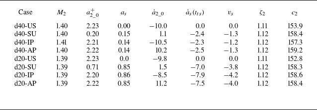
Detailed parameters for the interaction of the inner interface with the perturbed TS $_1$ . $M_2$ is the average Mach number of the perturbed TS $_1$ when it collides with the inner interface; $a^{+}_{2\_0}$ is the post-shock amplitude of the inner interface; $a_s$ is the amplitude of the perturbed TS $_1$ ; ${\dot a}_{2\_0}$ is the initial growth rate of the inner interface immediately after the impact of TS $_1$ (measured from experiment); ${{\dot a}_{s}}(t_{ts})$ is the growth rate of the amplitude of rippled TS $_1$ ; $v_s$ is the average growth rate induced by velocity perturbation; $\zeta _2$ is the specific heat ratio of the SF $_6$ layer; $c_2$ is the sound speed of the SF $_6$ layer; the units are mm and m s⁻¹ for the length and growth rate, respectively.

To account for the baroclinic vorticity regime, an initial vortex sheet generated immediately after the shock–interface interaction should be accurately calculated. Here, the initial vortex sheet strength at the inner interface, generated by the impact of the rippled TS $_1$ , can be calculated using (4.12). Then, we consider the velocity perturbation regime. In the case of a rippled shock, the shock strength varies continuously along its surface (i.e. stronger at the crest and weaker at the trough), resulting in a non-uniform velocity jump of the interface caused by the shock impact. This differs from the case of an unperturbed shock, where the interface acquires a uniform velocity immediately after the shock passage. According to the analysis of Ishizaki et al. (Reference Ishizaki, Nishihara, Sakagami and Ueshima1996), the velocity perturbation caused by a rippled shock can be estimated as

(4.14) \begin{equation} {v_{s}(t_{0})} =\frac {{\unicode{x0394} V}}{V_s} {{\dot a}_{s}}(t_{0}), \end{equation}

where $\unicode{x0394} V$ is the velocity jump of the interface, $V_s$ is the average velocity of the shock and $\dot {a}{_s}(t{_0})$ is the growth rate of the amplitude of the rippled shock just before its collision with the inner interface. The calculation results for all cases are listed in table 2. Note that the inner interface, which is of a heavy/light configuration, first undergoes phase inversion and then exhibits instability growth. In an anti-phase layer, ${\dot a}_{s}{\dot a}_{2}\lt 0$ , indicating that phase inversion is inhibited by the rippled TS $_1$ . Conversely, in an in-phase layer, ${\dot a}_{s}{\dot a}_{2}\gt 0$ , meaning that the rippled TS $_1$ acceleration phase undergoes inversion. This effect is more pronounced in thin layers, while it is significantly weaker in thick layers, as indicated by table 2. The reason is given below. For thick layers ( $d = 40$ mm), the amplitude of the rippled shock is very small when it arrives at the inner interface and can be approximated as a uniform cylindrical shock. In the case of a uniform shock, ${\dot a}{_s} = 0$ and ${v_{s}} = 0$ , meaning that the velocity perturbation is absent. In contrast, for thin layers ( $d = 20$ mm), the amplitude of the rippled TS $_1$ is evident when it arrives at the inner interface, producing considerably large velocity perturbation. This indicates that the layer thickness is crucial, as it not only governs the strength of the interface coupling effect but also influences the evolution of the distorted transmitted shock, which in turn affects the evolution of the inner interface.

To provide further theoretical insight, the oscillation frequency for the TS $_1$ in the current experiments is calculated. According to Calvo-Rivera et al. (Reference Calvo-Rivera, Velikovich and Huete2023) and Bates (Reference Bates2012), the oscillation frequency for a corrugated-piston-driven planar shock is given by

(4.15) \begin{equation} {\begin{array}{c} \omega _s = k_s\sqrt {c_2^2-u_2^{* 2}}, \end{array}} \end{equation}

where $k_s=2\pi /\lambda _s$ is the spatial wavenumber of the rippled shock, with $\lambda _s$ being the spatial wavelength. Here, $c_2$ and $u_2^{*}$ are the post-shock speed of sound and the velocity of shock movement relative to the compressed gas, respectively. For a convergent, sinusoidally distorted shock, there is $\lambda _s=2\pi R_{s\_i}/n$ . Based on this formula, the oscillation frequency of a perturbed converging shock increases as the radius decreases. This arises from the inability to associate the shock dynamics with a single characteristic length in the length-free problem. For instance, Huete et al. (Reference Huete, Velikovich, Martínez-Ruiz and Calvo-Rivera2021) and Calvo-Rivera et al. (Reference Calvo-Rivera, Huete and Velikovich2022) discussed expanding shocks, where shock oscillation frequency decreases due to geometric divergence. Here, the oscillation period of TS $_1$ is calculated by $T_s=2\pi /\omega _s$ . For case d40-SU, $T_s$ is approximately 710 $\unicode {x03BC}$ s at $R_{s\_i}=280$ mm (outer interface) and 636 $\unicode {x03BC}$ s at $R_{s\_i}=240$ mm (inner interface). The time interval for TS $_1$ to propagate between these interfaces is $\unicode{x0394} T \approx 165$ $\unicode {x03BC}$ s, which is approximately a quarter of the first oscillation period. It suggests that the amplitude of TS $_1$ approaches zero when it reaches the inner interface. This result aligns with the experimental schlieren images in figure 4, where the inner interface in case d40-SU remains perfectly cylindrical after interaction with TS $_1$ . As shown in figure 6 $(b)$ , the instability growth at the inner interface remains consistent for other thick layer cases (d40-US, d40-IP and d40-AP), suggesting that the amplitude of TS $_1$ is effectively zero at the inner interface in these cases. For case d20-SU, $T_s$ is approximately 693 $\unicode {x03BC}$ s at $R_{s\_i}=280$ mm (outer interface) and 655 $\unicode {x03BC}$ s at $R_{s\_i}=260$ mm (inner interface). The time interval $\unicode{x0394} T \approx 85$ $\unicode {x03BC}$ s is less than a quarter of the first oscillation period, illustrating a visible perturbation at TS $_1$ prior to its interaction with the inner interface.

Considering the effect of the rippled TS $_1$ , the radial component of the velocity of the inner interface can be expressed as

(4.16) \begin{equation} {\begin{array}{c} {{u}_{\infty }^m}= {{v}_c(t)}+{{v_s}}\cos (n \theta ), \end{array}} \end{equation}

where ${v}_c(t)$ is the time-dependent radial velocity component of the entire interface induced by the shock. In this work, ${v}_c(t)$ is calculated using the first time-derivative of the interface position measured from experiment and $v_s$ is calculated using (4.14). Note that in cylindrical geometry, the velocity vector at each position on the interface directs to the geometric centre, namely its direction varies with $\theta$ . Thus, the velocity vector can be expressed as

(4.17) \begin{equation} {\begin{array}{c} {\boldsymbol {u}_{\infty }^m}(\theta , t)={ \boldsymbol {v}_c(\theta , t)}+{\boldsymbol {v_s}(\theta , t)}\cos (n \theta ). \end{array}} \end{equation}

By incorporating the above equation into (4.4), a new vortex method that accounts for the effect of TS $_1$ is obtained, which is referred to as the vortex-b-m method.

Table 3.

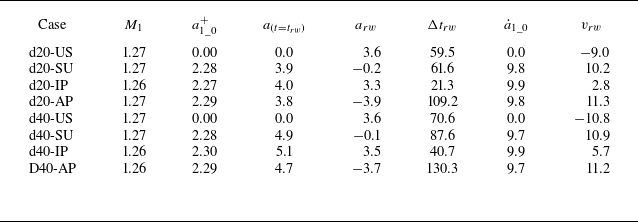
Detailed parameters for the interactions of the outer interface with the ICS and RW. $M_1$ is the Mach number of ICS; $a^{+}_{1\_0}$ is the interface amplitude shortly after the passage of ICS (obtained from experiment); $a_{(t=t_{rw})}$ is the amplitude of the outer interface at the time $t_{rw}$ ; $a_{rw}$ is the amplitude of the RW; $\unicode{x0394} t_{rw}$ is the time duration for RW passing through the outer interface; ${\dot a}_{1\_0}$ is the initial growth rate of the outer interface after the impact of ICS; ${v}_{rw}$ is the average growth rate of the outer interface induced by RW; the units are $\unicode {x03BC}$ s, mm and m s⁻¹ for the time, length and growth rate, respectively.

Next, we examine the influence of the rippled RW on the outer interface. A recent study (Zhang et al. Reference Zhang, Ding, Li, Zou and Luo2023a ) demonstrated that a rarefaction wave affects instability growth in two primary ways: it stretches the interface, thereby directly amplifying its amplitude, and it accelerates the background flow, producing RT stability or instability that suppresses or enhances the instability growth. First, we consider the stretching effect. Assuming the RW stretches the outer interface evenly, an empirical formula for the perturbation growth rate ( $\boldsymbol {v}_{rw}$ ) caused by wave stretching was derived by Zhang et al. (Reference Zhang, Ding, Si and Luo2023b ). It is formulated as

(4.18) \begin{equation} {\begin{array}{c} {v_{rw} }=\left \{\begin{array}{l} \dfrac {\unicode{x0394} a^{rw}_2}{\unicode{x0394} t_{rw}}=\dfrac {\unicode{x0394} t_s\left(\unicode{x0394} V_1^*-\unicode{x0394} V_1\right)/2}{\vert \unicode{x0394} t_s \vert +\unicode{x0394} t_g} \qquad \left(t_{rw}\lt t\lt t_{rw}+\unicode{x0394} t_{rw}\right) \\[4 mm] 0 \qquad \qquad \qquad \qquad \qquad \qquad \qquad (\text {others}) \end{array}\right . \\[5mm] \end{array}}, \end{equation}

where $t_{rw}$ is the time when the RW encounters the interface, $\unicode{x0394} t_{rw}$ is the time duration for the RW passing through the interface, $\unicode{x0394} a^{rw}_2$ is the amplitude increment caused by the stretching effect, $\unicode{x0394} V_1^*$ is the average velocity of the interface impacted by the RW, and $\unicode{x0394} t_{s}$ is the time duration between the moments when the crest and trough of the leading front of RW encounter the interface. The calculation results for all cases are listed in table 3.

Then, we examine the effect of interface acceleration caused by RW. This is achieved by incorporating the time-dependent interface velocity, $\boldsymbol {v}_c(\theta , t)$ , which is approximated by the first time-derivative of the interface trajectory measured from experiment, into the background velocity. Considering both the acceleration and stretching effects caused by RW, the background velocity is changed to

(4.19) \begin{equation} {\begin{array}{c} {\boldsymbol {u}_{\infty }^m}(\theta , t)={ \boldsymbol {v}_c(\theta , t)}+{\boldsymbol {v_{rw}}(\theta , t)}\cos (n \theta ). \end{array}} \end{equation}

Incorporating the above equation into (4.4), a new vortex method that considers the effect of RW is obtained. In this work, the vortex method, in which the background velocity involves the effects of waves, i.e. either (4.17) for TS $_1$ or (4.19) for RW, is generally referred to the vortex-b-m method.

Comparisons of the interface morphology evolution between the experiment and the vortex-b-m method for both thick and thin layers are given in figures 8 and 9, respectively. As we can see, the vortex-b-m method well reproduces the deformation of thick layers from linear to nonlinear stages, indicating that the current vortex model effectively captures the primary driving mechanisms behind instability growth in thick layers. However, for thin layers, the predictions of the vortex-b-m method evidently deviate from the experimental results, particularly at late stages, as illustrated in figure 9. Notably, in the case of d20-IP, the prediction suggests an intersection of the two interfaces, which is physically implausible. This discrepancy arises because the vortex-b-m method does not account for interface coupling effects, a crucial factor in the evolution of thin layers, as discussed in § 3.

Figure 8.

Comparison of the interface profile among the experiment (bold black line in the middle of each image), the vortex-b-m model (blue line at the bottom), and the vortex-b-m-c model (red line at the top) for cases d40-AP and d40-IP. The unit of numbers is $\unicode {x03BC}$ s.

Figure 9.

Comparison of the interface profile among the experiment (bold black line in the middle of each image), the vortex-b-m model (blue line at the bottom), and the vortex-b-m-c model (red line at the top) for cases d20-AP and d20-IP. The unit of numbers is $\unicode {x03BC}$ s.

4.4. Involving interface coupling effect

Under the assumption of incompressible, irrotational flow, the influence of interface coupling on instability growth in the linear regime has been theoretically analysed by Mikaelian (Reference Mikaelian1995, Reference Mikaelian2005). However, extending these theoretical models to the nonlinear stage is challenging, as nonlinearity greatly increases the complexity of the problem. In particular, during the nonlinear stage of convergent RM instability, interface coupling effect could interact with other factors, such as geometric contraction and reverberating waves, further complicating the problem. So far, the influence of interface coupling on instability growth at the nonlinear stage, whether in planar or cylindrical geometry, has not been fully assessed. Unlike existing models, the vortex method can straightforwardly incorporate the effects of interface coupling by simultaneously considering the motion and transport of multiple vortex sheets at each time step. Considering this, the Lagrangian velocity of a fluid point at either interface is influenced by all the vortex sheets:

(4.20) \begin{equation} {u}-i{v}=\frac {i}{2 \lambda } \left({\int \limits _{\boldsymbol {S_1}}}+{\int \limits _{\boldsymbol {S_2}}}+\ldots +{\int \limits _{\boldsymbol {S_N}}}\right) \gamma ' \cot \frac {\pi (z-{z}')}{\lambda } {\rm d} {s}'. \end{equation}

In the equation above, the integral path for each vortex sheet (e.g. $S_1$ , $S_2$ ) is defined along the sheet itself, encompassing all Lagrangian points on that sheet. In the absence of interface coupling effects, the velocity of any point on a vortex sheet is determined solely by integrating along that sheet. For example, the velocity of a point on $S_1$ would only require integration over $S_1$ . However, when interface coupling is considered, the velocity calculation must account for contributions from all vortex sheets. For instance, in the double-interface configuration studied in our experiments, the velocity of a point on the inner interface $S_1$ is calculated as the sum of (i) the self-induced velocity obtained by integrating over all points on $S_1$ and (ii) the induced velocity from the outer interface obtained by integrating over all points on $S_2$ . The vortex method adopting (4.20) is referred to as the vortex-b-m-c method.

Comparisons of the layer morphology evolution among the experiment, the vortex-b-m method and the vortex-b-m-c method for thick and thin layers are presented in figures 8 and 9, respectively. For thick layers, both vortex methods yield nearly identical predictions due to the weak interface coupling there. However, for thin layers, the vortex-b-m-c method provides significantly better predictions compared with the vortex-b-m method. Particularly, at late stages when the two interfaces are nearly merging, the vortex-b-m-c method provides a more accurate prediction of the interface behaviour. The good agreement between the experiment and the vortex-b-m-c method highlights the significant role of interface coupling in the evolution of thin layers. As seen in figure 9, the vortex-b-m method exhibits a small roll-up at the late stage in the d20-AP case (709 $\unicode {x03BC}$ s), which is not observed in either the experiment or the prediction of the vortex-b-m-c method. This suggests that interface coupling inhibits the formation of roll-ups in an anti-phase layer. Additionally, the predicted interface morphology tends to be flatter (with smaller amplitude) for the IP case compared with the SU or US cases, while it shows a sharper structure (with larger amplitude) for the AP case. This observation is qualitatively consistent with the analysis of interface coupling at the linear stage of cylindrical RM instability (Mikaelian Reference Mikaelian2005).

Quantitative comparisons in the amplitude growths of the inner and outer interfaces among the experiment, the vortex-b-m method, and the vortex-b-m-c method are given in figure 10. For thick layers, both vortex methods provide reasonable predictions of instability growth, albeit with varying degrees of accuracy. Notably, for case d40-IP, the vortex-b-m method shows better agreement with experimental data for the outer interface compared with the vortex-b-m-c method, as shown in figure 10(a). This discrepancy can be attributed to two main factors. First, the vortex-b-m-c method assumes incompressible flow, where vorticity information propagates instantaneously between interfaces. However, in real flows, vorticity disturbances propagate at the speed of sound. For thick layers with widely separated interfaces, the time required for vorticity disturbance propagation becomes significant. As a result, the vortex-b-m-c method may overestimate the suppression effect for IP cases, as the actual coupling between distant interfaces is weaker than the model assumes. Second, despite the careful design of the experimental set-up, unavoidable factors such as the presence of thin filaments used to form the interfaces and three-dimensional effects may introduce measurement inaccuracies. These experimental uncertainties could make the simpler vortex-b-m method appear more accurate in some cases. In contrast, for thin layers where interfaces are sufficiently close, the vorticity propagation time is negligible, approximately satisfying the incompressible assumption, and coupling effects are strong enough to outweigh experimental uncertainties. Consequently, the vortex-b-m-c method consistently provides better predictions than the vortex-b-m method, particularly at late stages. These observations underscore the importance of considering compressibility effects when modelling interface coupling in instability growth. Despite this, to the authors’ knowledge, this is the first accurate prediction of convergent RM instability at multiple interfaces across both linear and nonlinear stages. The present results exhibit great potential of the developed vortex method for studying the RM instability with complex physical factors such as geometric contraction, interface coupling and wave effects.

Figure 10.

Comparison of the amplitudes of the (a,c) outer and (b,d) inner interfaces between experiments and predictions for layers of various thicknesses and shapes. The dotted line refers to the prediction of vortex-b model, the dashed line to the prediction of vortex-b-m and the solid line to the prediction of the vortex-b-m-c model. Note the predictions of the vortex-b method for instability growth at the inner interface of thin layers nearly collapse with the prediction of vortex-b-m for case d20-US, and thus are not shown in (d).

The present vortex method demonstrates excellent predictive capability for the majority of our experimental conditions. Nevertheless, it is important to emphasise that its validity is bounded by specific physical assumptions. Specifically, this method is based on the assumptions of incompressible, irrotational and inviscid flow, as well as an idealised point vortex approximation. These assumptions are consistent with the conditions of weak shocks and discontinuous interfaces in our experiments. However, the vortex method requires further refinement to address a broader range of conditions. For instance, under strong shock conditions, the effects of compressibility and bulk vorticity become significant (Wouchuk & Nishihara Reference Wouchuk and Nishihara1997) and must be accounted for. Similarly, for diffusive interfaces, the use of vortex kernel distributions should be considered instead of relying on the idealised point vortex approximation. Moreover, the current implementation of our vortex method requires experimental inputs for the background flow and initial growth rates. This seems to limit its direct application to cases without experimental data. However, we would like to clarify several points. First, the requirement of experimental inputs is not a fundamental limitation of the method itself, but rather a practical choice in the current implementation. The background flow could alternatively be obtained from theoretical analysis or numerical simulations. Second, for simple configurations where analytical solutions exist for initial growth rate and background flow (e.g. single-mode RM instability in planar geometry), our method can directly use these solutions without requiring experimental inputs. The need for experimental data primarily arises in convergent geometry where exact analytical solutions are currently unavailable. Third, the main contribution of our work is demonstrating how various physical effects (background flow, interface coupling, reverberating waves) can be incorporated into the vortex method framework. This framework can be adapted to other configurations by modifying the input parameters accordingly.