1. Introduction
Sedimentation/suspension and fluidization are found in many natural and industrial systems such as wastewater treatment, chemical processes and sediment transport. In wastewater treatment, sedimentation is used to separate, through settling, both grit and organic particles (Burton et al. Reference Burton, Tchobanoglous, Tsuchihashi and David Stensel2013; Scherson, Woo & Criddle Reference Scherson, Woo and Criddle2014) and fluidized-bed reactors are widely used in treating both industrial and domestic wastewater (Shin et al. Reference Shin, McCarty, Kim and Bae2014; McCarty Reference McCarty2018; Shin & Bae Reference Shin and Bae2018). More recently, fluidized particles have been used to reduce biological membrane fouling (Shin et al. Reference Shin, Kim, McCarty, Kim and Bae2016). In these applications, predicting the settling velocity in sedimentation or upflow velocity in fluidization provides valuable information for system design and operation.
Over the years, the general consensus has been to use a power-law model that relates the volume fraction  $\phi$ to the velocity of interest
 $\tilde {U}$ (settling velocity in sedimentation and upflow velocity in fluidization) (Richardson & Zaki Reference Richardson and Zaki1954; Garside & Al-Dibouni Reference Garside and Al-Dibouni1977; Di Felice Reference Di Felice1995; Yin & Koch Reference Yin and Koch2007; Willen & Prosperetti Reference Willen and Prosperetti2019). The power law has been widely verified to be of the form
 \begin{equation} \dfrac{\tilde{U}}{w^*} = (1-\phi)^n, \end{equation}
where  $\tilde {U}$ is the hindered settling velocity,
 $w^*$ is the reference terminal velocity of a single particle in the domain of interest and
 $n$ is the expansion index or power-law exponent (Richardson & Zaki Reference Richardson and Zaki1954; Garside & Al-Dibouni Reference Garside and Al-Dibouni1977). In early studies, the main focus was to accurately model
 $n$ as a function of the terminal Reynolds number in the domain of interest
 $Re^*_{t}=w^*d_p/\nu _f$, where
 $d_p$ is the particle diameter and
 $\nu _f$ is the fluid kinematic viscosity. Defining
 $U_t$ as the terminal velocity of a single particle in a finite-sized domain and
 $U_{t,\infty }$ as that in an infinitely large domain, a stepwise relationship between
 $n$ and
 $Re_{t,\infty } = U_{t,\infty }d_p/\nu _f$ was proposed by Richardson & Zaki (Reference Richardson and Zaki1954) by using experimental data with concentrated volume fraction (
 $\phi > 0.05$) as
 \begin{equation} n =\begin{cases} 4.65, & Re_{t,\infty} < 0.2,\\ 4.35Re_{t,\infty}^{{-}0.03}, & 0.2 \leqslant Re_{t,\infty} < 1,\\ 4.45Re_{t,\infty}^{{-}0.1}, & 1 \leqslant Re_{t,\infty} < 500,\\ 2.39, & Re_{t,\infty}\geqslant 500. \end{cases} \end{equation}
Garside & Al-Dibouni (Reference Garside and Al-Dibouni1977) improved the relationship with a continuous sigmoid function proposed to relate the expansion exponent  $n$ to
 $Re_{t}= U_td_p/\nu _f$ as
 \begin{equation} n = \dfrac{5.1 + 0.27Re_t^{0.9}}{1 + 0.1 Re_t^{0.9}},\end{equation}
which was found to improve the accuracy of the power law by 20 %–30 % (Yin & Koch Reference Yin and Koch2007). As  $Re_t$ and
 $Re_{t,\infty } \rightarrow 0$,
 $n\rightarrow 4.65$ in (1.2) and 5.1 in (1.3).
Batchelor (Reference Batchelor1972), on the other hand, predicted the theoretical hindered settling velocity of monodispersed particles for a dilute suspension in viscous flow and showed that  $n$ would be 6.5 for small Péclet number and 5.5 for large Péclet number suspensions (Batchelor & Wen Reference Batchelor and Wen1982), where the Péclet number is a ratio of the relative effects of gravity to Brownian diffusion. Di Felice (Reference Di Felice1999) discovered that
 $n$ is the same in both dilute and concentrated suspension in the viscous regime (
 $Re_t \ll 1$) which is supported by computing
 $n$ in the limit of large Péclet number in (1.3). However,
 $n$ becomes approximately 1.5 times smaller in concentrated suspensions for intermediate terminal Reynolds numbers, leading to a lower hindered settling velocity in concentrated suspensions. This indicates a deceleration as the volume fraction transitions from dilute to concentrated suspensions. If there was no deceleration in the concentrated regime,
 $n$ would be the same for both regimes over all Reynolds numbers. To address this discrepancy in the hindered settling velocity, many researchers (Di Felice Reference Di Felice1995, Reference Di Felice1999; Yin & Koch Reference Yin and Koch2007; Hamid, Molina & Yamamoto Reference Hamid, Molina and Yamamoto2014; Zaidi, Tsuji & Tanaka Reference Zaidi, Tsuji and Tanaka2015; Willen & Prosperetti Reference Willen and Prosperetti2019) proposed to include a prefactor
 $k$ that typically ranges from 0.8 to 0.9 and proposed the modified power law
 \begin{equation} \dfrac{\tilde{U}}{w^{\ast}} = k(1-\phi)^n. \end{equation}
In addition, as  $Re_t$ increases, the prefactor
 $k$ for the power-law model that is satisfied for both the dilute and concentrated suspensions also decreases (Yin & Koch Reference Yin and Koch2007). Some studies also suggest
 $k$ in the range 0.8–0.9 for concentrated suspensions (
 $\phi > 0.05$) (Chong, Ratkowsky & Epstein Reference Chong, Ratkowsky and Epstein1979; Di Felice Reference Di Felice1995). Di Felice (Reference Di Felice1995) conjectured that this discrepancy might be correlated to the size of particles.
Many studies have shown that particles tend to form clusters in dilute suspensions (Li et al. Reference Li, Xia, Tung and Kwauk1991; Uhlmann & Doychev Reference Uhlmann and Doychev2014; Capecelatro, Desjardins & Fox Reference Capecelatro, Desjardins and Fox2015; Fullmer & Hrenya Reference Fullmer and Hrenya2017). The first mechanism is cluster-induced turbulence (known as CIT) which occurs when the system has a mass loading  $\psi \gg 1$, where
 $\psi$ is defined as
 \begin{equation} \psi = s\dfrac{\phi}{1-\phi}, \end{equation}
where  $s=\rho _p/\rho _f$ is the particle to fluid density ratio and
 $\rho _p$ and
 $\rho _f$ are the respective particle and fluid densities. In most experiments conducted to correlate
 $n$ and
 $k$ to
 $Re_t$ (Richardson & Zaki Reference Richardson and Zaki1954; Garside & Al-Dibouni Reference Garside and Al-Dibouni1977; Yin & Koch Reference Yin and Koch2007; Willen & Prosperetti Reference Willen and Prosperetti2019),
 $s\sim O(0.1 - 1)$, and hence cluster-induced turbulence is unlikely to occur. Another cluster formation mechanism is wake interaction. Wake interactions are observed when the Archimedes number
 $Ar$ or Galilei number
 $Ga$ exceed some threshold (Uhlmann & Doychev Reference Uhlmann and Doychev2014) where
 $Ar$ and
 $Ga$ are defined as
 \begin{equation} Ar = Ga^2 = \dfrac{g(s-1)d_p^3}{\nu_f^2}, \end{equation}
where and  $g$ is the gravitational acceleration. Most of the studies on particle clustering focus on dilute instead of concentrated suspensions. To date, no explanations have been provided to address the deviation of
 $k$ from unity in concentrated suspensions. Therefore, a better understanding of the mechanisms governing and affecting
 $k$ is required. For the remainder of this paper, the reference velocity in (1.1) and (1.4) will be denoted as
 $U_t$, the settling velocity of a single particle in the domain of interest, since the simulations are conducted in periodic domains without wall effects.
While sedimentation and fluidization can be studied with experiments or simulations, the advantage of experiments is the ability to test a large number of different particle parameters which is beneficial for establishing a relationship between  $Re_t$ and
 $n$. However, the main disadvantage of experiments is the difficulty in tracking individual particle information over time, leading to challenges in understanding both the fluid microstructure and microscopic particle behaviour. High-fidelity particle resolved simulations (PRS) simulate the movement of particles over time by resolving the flow around each particle, enabling accurate quantification of fluid–particle interactions. Therefore, tracking information of individual particles over time is possible, which enables the examination of microstructure and improves understanding of the mechanisms governing particle motion.
To understand the dependence of the prefactor  $k$ on different non-dimensional parameters, a formal dimensional analysis is conducted. We consider a case when a cloud of particles is settling or fluidized with volume fraction
 $\phi$ in a periodic domain of horizontal extent
 $L$. The hindered/superficial velocity is related to six dimensional parameters and the non-dimensional volume fraction
 $\phi$ with
 \begin{equation} \tilde{U} = f(d_p, \nu_f, \rho_f, \rho_p, g, L, \phi). \end{equation}
Dimensional analysis results in a total of four dimensionless groups. Choosing  $\rho _p$,
 $\nu _f$ and
 $d_p$ to non-dimensionalize the other parameters results in the functional relationship
 \begin{equation} Re_p = f(\phi, Ar, s, d_p/L), \end{equation}
where the particle Reynolds number is defined as
 \begin{equation} Re_p = \dfrac{\tilde{U}d_p}{\nu_f}. \end{equation}
For the range of density ratios of interest, we will show that the results weakly depend on  $s$. Furthermore, in a sufficiently large periodic domain, the dependence on
 $d_p/L$ vanishes. Therefore, the only parameters governing the particle Reynolds number are
 $\phi$ and
 $Ar$, implying
 \begin{equation} Re_p = f(\phi, Ar). \end{equation}
Therefore, we expect any non-dimensional parameter, including the prefactor  $k$ in (1.4), to depend on just two non-dimensional parameters. Since the literature suggests that the term
 $(1-\phi )^n$ in (1.4) largely captures the effects of
 $\phi$, we can further assume that
 $k$ depends primarily on one parameter, namely
 $Ar$.
In this paper, we use PRS of monodispersed particle suspensions to understand the effects of the Archimedes number and particle density ratio on the hindered settling velocity. A series of simulations are analysed to understand the relationship between  $Ar$ and the prefactor
 $k$ in (1.4), and we explain the results in the context of detailed fluid-particle physics.
2. Numerical methodology and simulation set-up
2.1. Equations and discretizations
The governing Navier–Stokes equations are solved in a three-dimensional cubic domain containing an array of uniform spherical particles. To enforce no-slip boundary conditions on the particle surfaces, a source term,  ${\boldsymbol {f}}_{{IBM}}$, based on the direct-forcing immersed boundary method (IBM) method is added to the incompressible Navier–Stokes equation to give
 \begin{equation} \frac{\partial\boldsymbol{u}}{\partial t} + \boldsymbol{u} \boldsymbol{\cdot} {\boldsymbol{\nabla}}{\boldsymbol{u}} ={-}\boldsymbol{\nabla}{p} + \nu_f \nabla^2{\boldsymbol{u}} + \boldsymbol{f}_{{IBM}}, \end{equation}
subject to continuity,  $\boldsymbol {\nabla }\boldsymbol {\cdot }{\boldsymbol {u}} = 0$, where
 $\boldsymbol {u}$ is the velocity vector and
 $p$ is the pressure normalized by the fluid density,
 $\rho _f$. These equations are discretized on a uniform collocated Cartesian grid. A fractional step method (Zang, Street & Koseff Reference Zang, Street and Koseff1994) is used to couple the momentum and pressure. The advection term is discretized with the explicit, three-step Runge–Kutta scheme described in Rai & Moin (Reference Rai and Moin1991). The viscous term is discretized with the implicit Crank–Nicolson scheme to eliminate the associated stability constraint. The linear systems arising from the implicit discretization of the viscous terms and the pressure Poisson equation are solved using the HYPRE library (Chow, Cleary & Falgout Reference Chow, Cleary and Falgout1998; Falgout & Yang Reference Falgout and Yang2002). To solve the interactions between the fluid and the particles, the direct forcing approach first proposed by Uhlmann (Reference Uhlmann2005) and improved by Kempe & Fröhlich (Reference Kempe and Fröhlich2012b) is adopted. Since the IBM formulation is unable to resolve the fluid–particle interactions when the particles are less than two grid cells apart, we follow the approach by Biegert, Vowinckel & Meiburg (Reference Biegert, Vowinckel and Meiburg2017) who employ the collision model proposed by Kempe & Fröhlich (Reference Kempe and Fröhlich2012a).
2.2. Numerical method validation
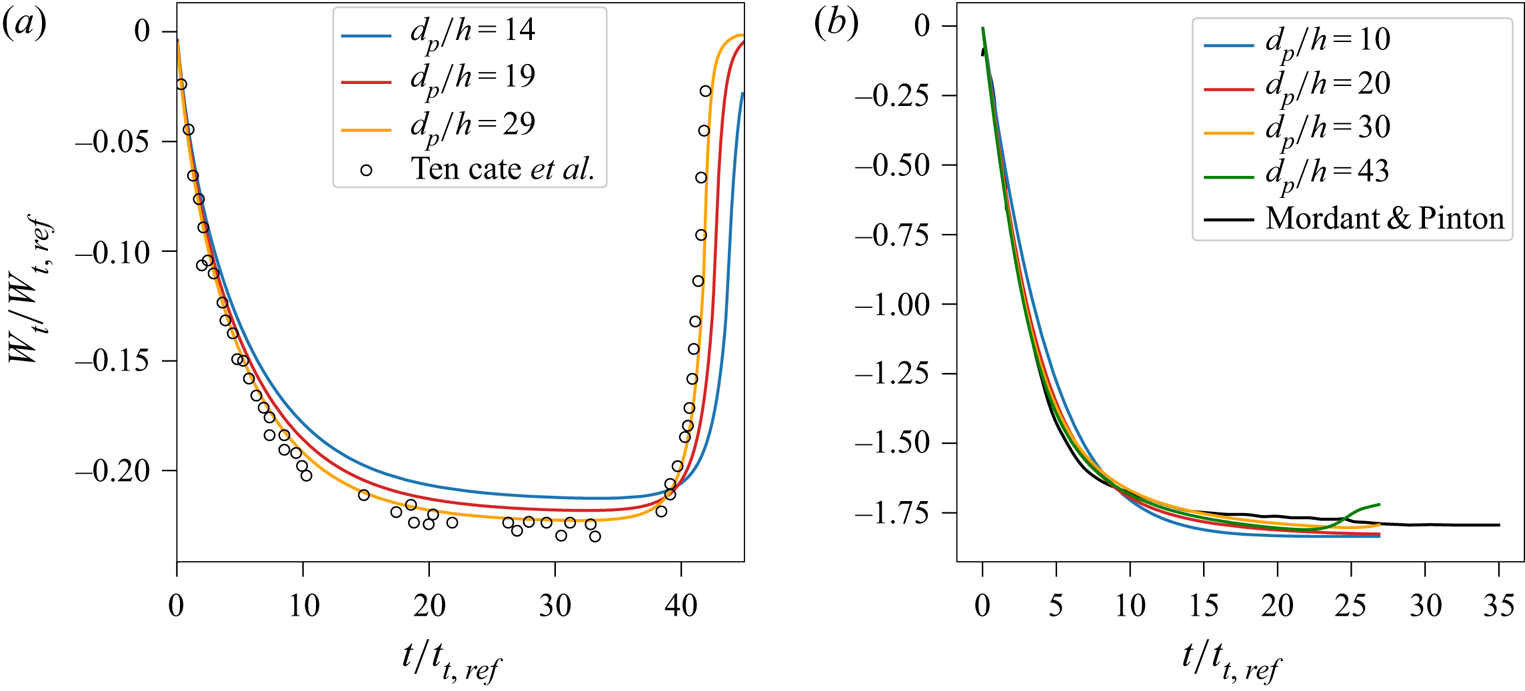
To test the methodology, we simulated a single particle settling in a three-dimensional domain with a quiescent fluid under the influence of gravity and compared the results with published values. Simulated particle settling is compared with the experimental result of ten Cate et al. (Reference ten Cate, Nieuwstad, Derksen and Van den Akker2002) (figure 1a) in which a particle settles in the negative  $z$-direction onto a bottom, no-slip wall, with
 $Re_t=12$. Particle settling is also compared with the results of Mordant & Pinton (Reference Mordant and Pinton2000) (figure 1b), in which a particle is allowed to come to terminal velocity with
 $Re_t=360$. The domain sizes are
 $6.66 d_p \times 6.66 d_p \times 13.33 d_p$ for the wall-bounded case and
 $7.5 d_p\times 7.5 d_p \times 60 d_p$ for the terminal settling case. The boundary conditions are periodic in all directions for the terminal settling case and periodic in the
 $x$- and
 $y$-directions with no-slip top and bottom walls for the wall-bounded cases. In all cases, a particle is initialized in the horizontal centre and
 $2d_p$ from the top of the domain with no vertical velocity in a quiescent fluid. The kinematic viscosity is
 $\nu _f = 1.175\times 10^{-4}\ \textrm {m}\ \textrm {s}^{-2}$ for the wall-bounded case and
 $\nu _f =5.416\times 10^{-3}\ \textrm {m}\ \textrm {s}^{-2}$ for the terminal settling case, and the fluid and particle densities are
 $\rho _f=1000$ and
 $\rho _p=1164\ \textrm {kg}\ \textrm {m}^{-3}$ (figure 1a) and
 $\rho _f=1000$ and
 $\rho _p=2560\ \textrm {kg}\ \textrm {m}^{-3}$ (figure 1b). The time-step size is dictated by requiring a maximum Courant number of
 $U_t\Delta t/h=0.5$, where
 $h=\Delta x = \Delta y = \Delta z$ is the grid spacing which is uniform in the
 $x$-,
 $y$- and
 $z$-directions. We perform simulations with different resolutions to determine the resolution needed to reproduce the published results. As shown in figure 1, for the wall-bounded case (figure 1a), the particle approaches its terminal settling velocity but then decelerates upon reaching the wall, while in figure 1(b) the particle reaches its terminal velocity. In both cases, the settling velocity is normalized by the reference velocity
 $w_{t,ref}=\sqrt {g d_p}$ and the time is normalized by the reference time
 $t_{t,ref}=\sqrt {d_p/g}$. The results indicate that our simulations agree with published results when
 $d_p/h=20 - 30$ grid points are used to resolve the flow around the particles, which is consistent with previous PRS simulations (Uhlmann Reference Uhlmann2005; Kempe & Fröhlich Reference Kempe and Fröhlich2012b; Biegert et al. Reference Biegert, Vowinckel and Meiburg2017).
Time series of the simulated settling velocity  $U_t$ of a single particle with (a)
 $Re_t=12$ and (b)
 $Re_t=360$ and different grid resolutions
 $h$ used to resolve the particle diameter
 $d_p$, compared with published results.

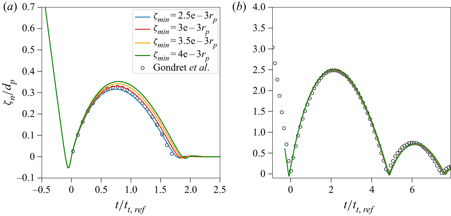
To validate the collision model, the simulation results were compared with the experiments of Gondret, Lance & Petit (Reference Gondret, Lance and Petit2002), in which a particle bounces off the wall of a tank. The experiments focus on the effect of the Stokes number on the maximum height of the particle after bouncing, where the Stokes number is defined as
 \begin{equation} St_{val} = \dfrac{\rho_p d_p u_{in}}{9\rho_f \nu_f}, \end{equation}
where  $u_{in}$ is the impact velocity. The parameters used in the simulations were identical to Biegert et al. (Reference Biegert, Vowinckel and Meiburg2017), and we simulate
 $St_{val}=27$ (figure 2a) and
 $St_{val}=152$ (figure 2b). The domain sizes in these simulations are
 $13.33 d_p\times 13.33 d_p \times 26.66 d_p$ for figure 2(a) and
 $6.67 d_p \times 6.67 d_p \times 66.7 d_p$ for figure 2(b), and
 $d_p/h=19.2$ grid points are used to resolve the particle diameter. The boundary conditions on the sidewalls are periodic with no-slip conditions on the top and bottom boundaries. Simulations are initialized with the particle at rest in a quiescent fluid with kinematic viscosity
 $\nu _f=1.036\times 10^{-4}\ \textrm {m}\ \textrm {s}^{-2}$ for figure 2(a) and
 $\nu _f=1.070\times 10^{-5}\ \textrm {m}\ \textrm {s}^{-2}$ for figure 2(b) and density ratio
 $s=8.083$ for figure 2(a) and
 $s=8.342$ for figure 2(b). Before reaching a distance
 $\zeta _n = d_p/2$ from the wall, the particle velocity is prescribed as the velocity in the
 $z$-direction
 \begin{equation} u(t) ={-}u_{in} (1-\textrm{e}^{{-}40t}). \end{equation}
The prescribed particle velocity is then removed when  $\zeta _n < d_p/2$, whereupon the particle is subject to velocity interactions with the fluid and wall. To account for lubrication effects, the collision model proposed by Biegert et al. (Reference Biegert, Vowinckel and Meiburg2017) requires a parameter dictating the minimum spacing between the particle and wall, setting the maximum lubrication force. Figure 2 shows the effect of different minimum spacing parameters and demonstrates that our results match the experiments when
 $\zeta _{min}=2.5\times 10^{-3} r_p$, where
 $r_p$ is the particle radius. We use this minimum distance in the collision model for all simulations in this paper.
Simulated height of the centre of a particle ( $\zeta _n$) bouncing off of a wall with (a)
 $St_{val}=27$ and (b)
 $St_{val}=152$ compared with published values. The minimum distance from the wall is
 $\zeta _{min}$.

2.3. Simulation set-up for particle clustering
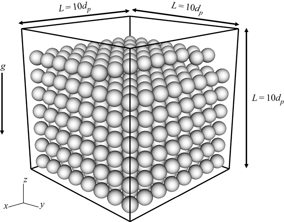
Three-dimensional simulations are conducted in a cubic, triply periodic domain, as shown in figure 3. The particles have a uniform diameter  $d_p=2$ mm and density
 $\rho _p$ that is varied to give different values of
 $s$, and the fluid has a density
 $\rho _f=998.21\ \textrm {kg}\ \textrm {m}^{-3}$. The grid spacing is uniform in all directions and given by
 $\Delta x=\Delta y=\Delta z=h=d_p/25.6$, which is sufficient to resolve the flow–particle interactions as demonstrated in § 2.2. The cubic domain has a side length
 $L = 10 d_p$, giving a three-dimensional grid with
 $256\times 256\times 256$ grid points. Yin & Koch (Reference Yin and Koch2007) showed that accurate PRS of particle suspensions with low
 $Re_t$ can be achieved with a cubic domain with
 $L \approx 10 d_p$ by applying a correction based on the structural factor (see § 3.3). The time step is determined based on the advection and diffusion Courant number which are defined as
 $C_{{adv}} = \tilde {U}\Delta {t}/h$ and
 $C_{{diff}} = \nu _f \Delta {t} / h^2$, respectively, resulting in a maximum Courant number
 $C_{max} = \max (C_{{adv}},C_{{diff}}) = 0.25$.
Initial particle positions in the periodic simulation domain with  $N_p = 817$ particles and a volume fraction
 $\phi = 0.43$.

Based on the dimensional analysis, the prefactor  $k$ is primarily a function of
 $Ar$, hence the parameter of interest is
 $Ar$ as defined in (1.6). To fit
 $n$ and
 $k$ using (1.4), simulations were conducted with three volume fractions
 $\phi = 0.22$,
 $0.30$,
 $0.43$, five Archimedes numbers
 $Ar = 21$,
 $100$,
 $1000$,
 $7413$, 23 600 and three density ratios
 $s = 1.3$,
 $2.46$,
 $6$. To obtain the desired volume fraction
 $\phi$, we compute the number of particles
 $N_p$ with fixed
 $L$ and
 $d_p$.
The desired values of  $Ar$ are achieved by varying the ratio of
 $(s-1)/\nu _f^2$ such that
 $N_p=434$,
 $581$,
 $817$ for
 $\phi = 0.22$,
 $0.30$,
 $0.43$. A total of 33 simulations were conducted as shown in table 1. All simulations are initialized with particles equally spaced in the domain (see figure 3) and the flow is initialized as static in all directions. The gravitational force leads to the settling and random motion of the particles until statistical equilibrium is reached, at which time the dynamics are independent of the initial particle distribution.
Summary of parameters used in the simulations. Each column represents parameters with different  $s$ while varying
 $\nu _f = [g(s-1)d_p^3/Ar]^{1/2}$ to ensure the desired
 $Ar$. Simulations with each
 $Ar$ and
 $s$ were conducted three times with different
 $\phi$ by varying
 $N_p$. The particle diameter and fluid density are held fixed at
 $d_p = 0.002$ m and
 $\rho _f = 998.21\ \textrm {kg}\ \textrm {m}^{-3}$, and the domain size is fixed at
 $L = 10 \ d_p$.

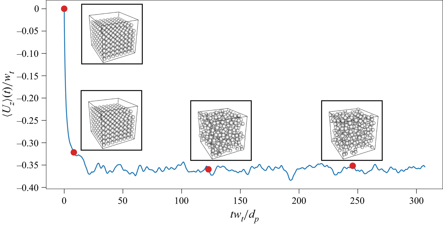
Defining the ensemble average over all particles with  $\langle \{ \boldsymbol {\cdot } \} \rangle$, figure 4 shows that the magnitude of the instantaneous ensemble settling velocity
 $\langle U_z \rangle$ initially increases with time as particles rearrange and settle. It eventually reaches statistical equilibrium once the average drag force in the vertical balances the weight of the particles. We compute the settling velocity of a single particle in an infinitely large domain,
 $U_t$ that satisfies the expression (Yin & Koch Reference Yin and Koch2007)
 \begin{equation} Ar =\begin{cases} 18 Re_t \left[ 1 + 0.1315 Re_t^{(0.82-0.05\log_{10}Re_t)} \right], & 0.01 < \Re_t < 20, \\ 18 Re_t \left[ 1 + 0.1935 Re_t^{0.6305} \right], & 20 < Re_t < 260. \end{cases} \end{equation}
Various researchers have shown that equation (2.4) has an error ranging from  $2\,\%$ to
 $4\,\%$ when compared with simulations of single particle settling in a periodic domain with
 $d_p/L$ ranging from
 $0.1$ to
 $0.05$. Yin & Koch (Reference Yin and Koch2007) have shown that as the size of domain
 $L$ increases and
 $d_p/L$ decreases,
 $U_t$ converges to the value calculated with (2.4). Therefore,
 $d_p/L = 0.1$ is sufficient to obtain results with error less than
 $4\,\%$. Simulations are run for
 $t_{max} = 200 - 500 \tau _T$ to obtain statistically converged results, where
 $\tau _T= d_p/U_t$ is defined as the particle turnover time. Time-average statistics are denoted by the overbar and computed over
 $50\tau _T$ such that
 \begin{equation} \overline{\{\boldsymbol{\cdot} \}}=\frac{1}{50\tau_T}\int_{t_i}^{t_{max}}\{\boldsymbol{\cdot} \}\,\textrm{d}t, \end{equation}
where  $t_i = t_{max} - 50\tau _T$. Using these definitions, the time-averaged ensemble settling velocity is given by
 $\langle \overline {U_z} \rangle$, which we refer to as the hindered settling velocity
 $\tilde {U}$ in what follows.
Time series of the ensemble settling velocity  $\langle U_z \rangle$ normalized by
 $U_t$ for
 $Ar=7413$,
 $s=1.3$ and
 $\phi =0.43$.

2.4. Evaluation of domain size
To evaluate the appropriateness of the domain size, we compute the two-point autocorrelation of Eulerian velocity fluctuations as
 \begin{equation} R_{u_i u_i}(r_j) = \dfrac{\langle u^\prime_i(x_{0,j} )u^\prime_i(x_{0,j} + r_j) \rangle}{\langle u^\prime_i(x_{0,j} )u^\prime_i(x_{0,j}) \rangle}, \end{equation}
where  $x_{0,j}$ is a reference point in the domain,
 $i$ and
 $j=x, y, z$ and
 $u^\prime _i = u_i - \langle u_i \rangle$ is the Eulerian velocity fluctuation and
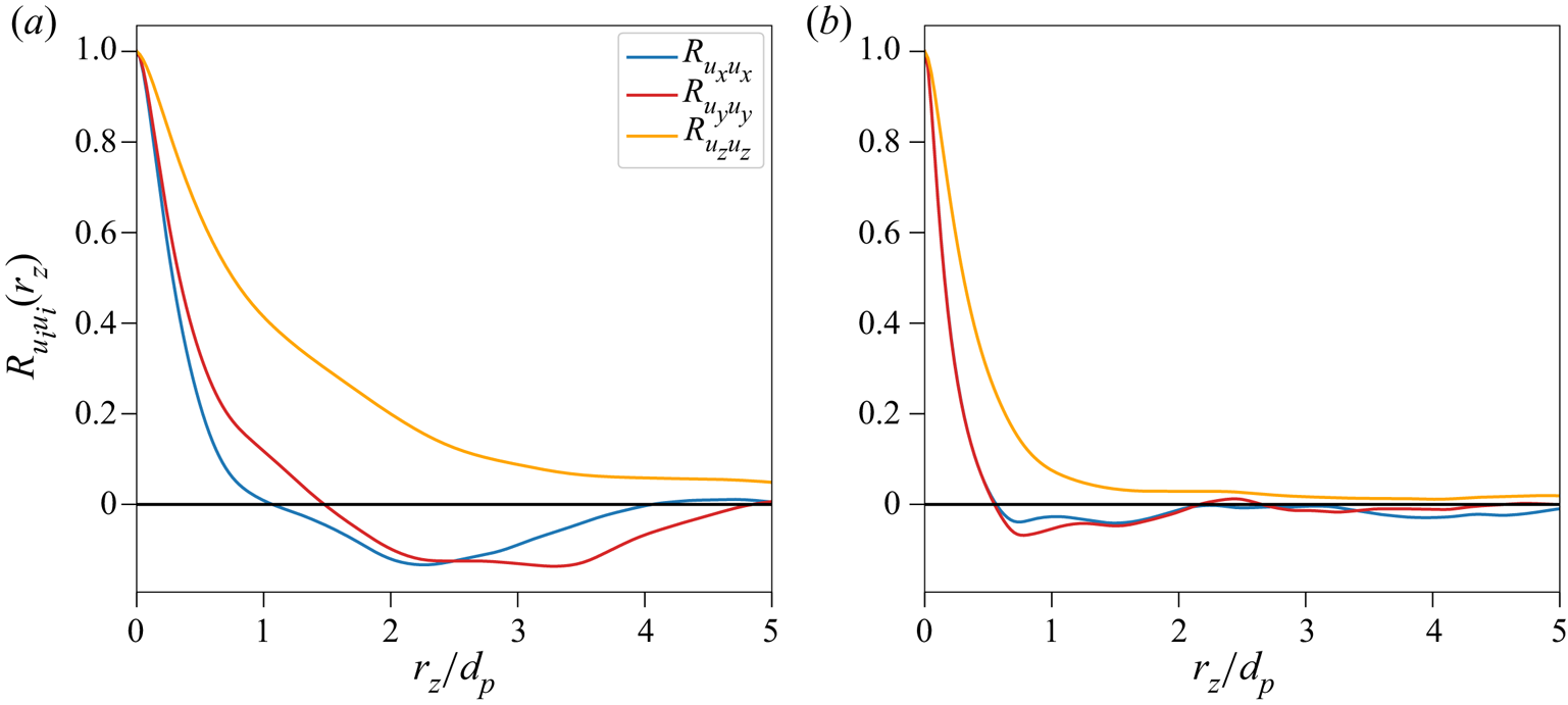
 $\langle u_i \rangle$ is the Eulerian spatially averaged velocity in all directions. Due to periodicity in all directions, we compute the two-point autocorrelation for half of the domain. Figure 5 shows the two-point autocorrelation as a function of
 $z$
 $R_{u_i u_i}(r_z)$ for cases with
 $Ar =21$ and 23 600. Overall, due to the presence of a mean flow in the
 $z$-direction, the decorrelation lengths are larger for fluctuations in
 $u_z$ than for
 $u_x$ and
 $u_y$. As
 $Ar$ increases, the decorrelation length decreases because the velocity fluctuations are more restricted to be local. For
 $Ar=21$ in the Stokes regime,
 $R_{u_zu_z}(r_z)$ decreases and converges to approximately 0.05, indicating nearly complete decorrelation. A similar trend is observed in the simulation by Uhlmann & Doychev (Reference Uhlmann and Doychev2014) with dilute suspensions of larger
 $Ar$ particles. The authors conclude that a further increase in domain size would not fully decorrelate the Eulerian velocity fluctuations. For the case of
 $Ar=23\,600$, the decorrelation lengths are approximately
 $2$ and
 $3 d_p$ for the respective transverse (
 $x$- and
 $y$-directions) and axial directions. With this analysis, we conclude that the domain size in this study is sufficient for complete decorrelation for high
 $Ar$ cases and nearly complete for low
 $Ar$ cases. For low
 $Ar$ cases, given the current trend where the slope of the two-point autocorrelation function is approximately zero, a further increase in domain size is unlikely to completely decorrelate the Eulerian velocity fluctuations. Nevertheless, the largest magnitude of the two-point autocorrelation
 $R_{u_zu_z}(r_z)$ is no bigger than approximately 0.05 for the case with the smallest value of
 $Ar$ in this study.
Two-point autocorrelation of Eulerian velocity fluctuations as a function of  $r_z$ for
 $Ar=$ (a)
 $21$ and (b) 23 600.

3. Results and discussion
3.1. Power-law behaviour and effect of Archimedes number on  $k$

For the cases with  $Ar=21$,
 $Re_t \approx 1$ results in Stokes law behaviour in which the finite periodic domain affects hindered settling velocity
 $\tilde {U}$. To correct the error associated with the finite domain size associated with Stokes flow, Yin & Koch (Reference Yin and Koch2007) used a correction method that relates the unbounded mean hindered settling velocity to the domain size with
 \begin{equation} \tilde{U} =\begin{cases} \langle \overline{U_z} \rangle + 1.7601 S_0 \dfrac{|{F}|}{3{\rm \pi} d_p \rho_f\nu_f^*}\left(\dfrac{\rm \pi}{6}\right)^{1/3} \left(\dfrac{d_p}{L}\right), & Ar \leqslant 21, \\ \langle \overline{U_z} \rangle, & Ar > 21, \end{cases} \end{equation}
where  $\langle \overline {U_z} \rangle$ is the hindered settling velocity in the bounded domain,
 $S_0$ is the structure factor in an unbounded suspension in the limit of zero wavenumber,
 $F = (\rho _p-\rho _f) {\rm \pi}d_p^3g/6$ is the buoyancy force of a single particle and
 $\nu _f^*$ is the apparent dynamic viscosity that can be approximated as (Ladd Reference Ladd1989)
 \begin{equation} \nu_f^* = \nu_f (1 + 2.5\phi + 5\phi^2). \end{equation}
Here,  $S_0$ is estimated using the Carnahan–Stirling approximation as
 \begin{equation} S_0 = \dfrac{(1-\phi)^4}{1+4\phi+4\phi^2- 4\phi^3+\phi^4} \end{equation}
which is applicable for  $\phi > 0.05$ (Yin & Koch Reference Yin and Koch2007).
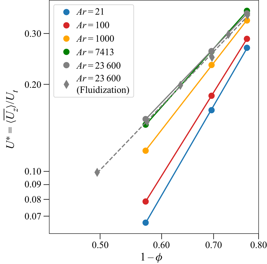
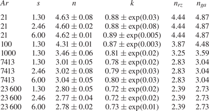
Table 2 and figure 6 show the least squares fit of the normalized average hindered settling velocity  $U^* = \langle \overline {U_z} \rangle /U_t$ to the power law given by (1.4). Also shown are results of fluidization in a doubly periodic domain with
 $N_p = 2000$ particles and
 $Ar=23\,600$ but with six values of
 $\phi$ (details in the Appendix). Since the regression of these results overlaps those in this paper, we are confident that three values of
 $\phi$ is sufficient to regress for
 $k$. In addition, each regression gives
 $n$ and
 $k$ values that fit equation (1.4) with coefficients of determination
 $R^2 = 1.0$. The fitted values of
 $n$ are consistent with the predictions from (1.2) and (1.3). Since the effects of the density ratio
 $s$ on
 $n$ and
 $k$ are negligible, from now on we report on results with
 $s = 1.3$ and ignore results with
 $s = 2.46$ and
 $6.0$.
Normalized hindered settling velocity  $u^*$ as a function of porosity
 $1-\phi$ for different Archimedes numbers
 $Ar$. Since the effect of the density ratio
 $s=\rho _p/\rho _f$ is negligible, we only show results for
 $s=1.3$. The dashed line is a regression based on six values of
 $\phi$ from simulations described in the Appendix.

Fitted expansion exponent,  $n$, and prefactor,
 $k$, along with 95 % confidence intervals that provide the best fits to equation (1.4). All fits have
 $R^2 = 1.0$.

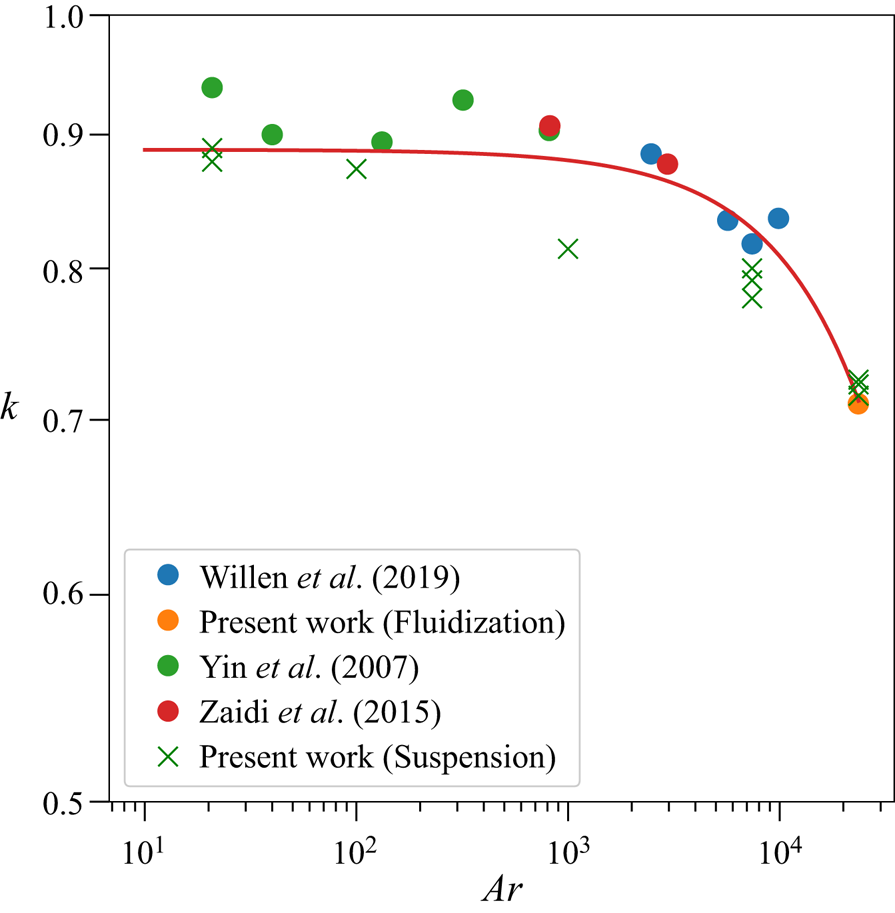
When plotted as a function of  $Ar$ as in figure 7, the magnitude of
 $k$ decreases as
 $Ar$ increases, indicating overprediction of
 $\tilde {U}$ with the original power-law equation (1.1). Therefore, a prefactor
 $k<1$ is needed to correct this overprediction. This result agrees with Di Felice & Parodi (Reference Di Felice and Parodi1996) and Chong et al. (Reference Chong, Ratkowsky and Epstein1979) that the prefactor
 $k$ should be included even for concentrated particle suspensions and also suggests that the mechanism leading to the overprediction is stronger for higher values of
 $Ar$. An exponential function of the form of
 $k = k_0 \exp (-\alpha Ar)$, where
 $k_0$ and
 $\alpha$ are fitted parameters, is used to fit the data shown in figure 7. After regression, the relationship between
 $k$ and
 $Ar$ fits the relation
 \begin{equation} k = 0.89\exp\left(-\frac{Ar}{10^5}\right), \end{equation}
with a coefficient of determination  $R^2 = 0.86$. As
 $Ar \rightarrow 0$,
 $k \rightarrow 0.89$. We note that (3.4) is only valid for the range of
 $Ar$ that we study (
 $21 \leqslant Ar \leqslant 2360$) and, while it reproduces the
 $Ar \rightarrow 0$ limit, it should not be used to interpret the
 $Ar \rightarrow \infty$ limit. According to Di Felice (Reference Di Felice1999), the relationship between hindered settling and the volume fraction can be accounted for by two sets of parameters for dilute and concentrated suspension, respectively. Comparing with concentrated suspensions,
 $n$ is higher to account for acceleration (Batchelor Reference Batchelor1972, Reference Batchelor1988) and
 $k = 1$ is used to recover
 $U_t$ as
 $\phi \rightarrow 0$ in dilute suspensions. In our work, since (1.4) fits with
 $\phi > 0.05$,
 $k \ne 1$ and decreases as
 $Ar$ decreases to account for lower hindered settling. This result agrees with various researchers (Di Felice & Parodi Reference Di Felice and Parodi1996; Yin & Koch Reference Yin and Koch2007; Willen & Prosperetti Reference Willen and Prosperetti2019). As
 $Ar \rightarrow \infty$ (turbulent regime), the effects of
 $Ar$ and
 $\phi$ on
 $n$ and
 $k$ are less well studied. Kowe et al. (Reference Kowe, Hunt, Hunt, Couet and Bradbury1988) suggests that
 $n \rightarrow 1.5$ as
 $Ar \rightarrow \infty$, although more work is required to understand the effects on
 $k$.
Prefactor  $k$ as a function of
 $Ar$ from various publications and the present work along with the best-fit curve given by (3.4).

3.2. Particle velocity fluctuations
We hypothesize that the lower hindered settling velocity at high  $Ar$ indicated by smaller
 $k$ is due to weaker particle clustering effects. Uhlmann & Doychev (Reference Uhlmann and Doychev2014) demonstrated the important effects of long-lived clusters for higher hindered settling velocity
 $u$ at moderate
 $Ar$ with low
 $\phi$. In our simulations, clusters persist for longer periods for lower
 $Ar$, implying that clustering will likely have more of an impact for low
 $Ar$ cases. On the other hand, particles collide more often and clusters are easily broken for higher
 $Ar$, implying that collisions will likely have more of an impact for high
 $Ar$.
To understand the details of the particle motions, we computed the variance of the vertical velocity fluctuation as
 \begin{equation} \langle \overline{U_z^{\prime 2}} \rangle = \langle \overline{(U_{z,n} - \langle U_z \rangle)^2} \rangle, \end{equation}
where  $U_{z,n}$ is the vertical velocity of particle
 $n=1,\ldots,N_p$. Figure 8 shows the variance of the vertical velocity fluctuations normalized by the square of the hindered settling velocity
 $\langle \overline {U_z} \rangle ^2$ as a function of
 $Ar$ for different
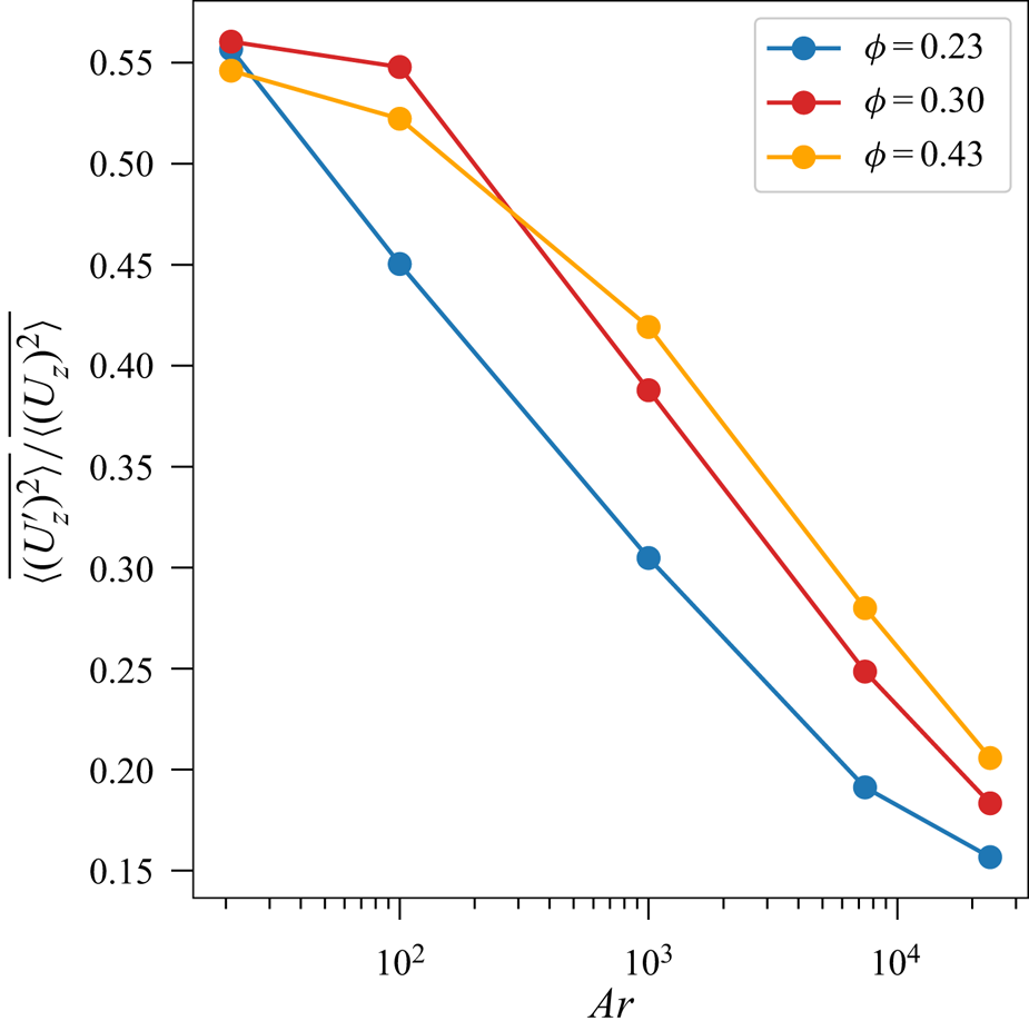
 $\phi$. In general, as
 $Ar$ increases, the normalized velocity fluctuation variance decreases possibly due to decreased wake interactions between particles at higher
 $Ar$. At high
 $Ar$, the effects of collisions (see § 3.5) dominate over the hydrodynamic forces, hence reducing the effect of wake interactions and normalized vertical velocity fluctuation variance. Interestingly, the lowest velocity fluctuation variance occurs when
 $\phi =0.43$ and
 $Ar = 21$, while this value of
 $\phi$ produces the largest variance when
 $Ar > 1000$.
Normalized vertical velocity fluctuation variance  $\langle \overline {(U_z^\prime )^2} \rangle /\langle \overline {(U_z)^2} \rangle$ as a function of
 $Ar$ for different
 $\phi$.

3.3. Frequency spectrum of particle velocity fluctuations
As discussed in § 3.2, the largest normalized vertical velocity fluctuation variance is observed at the lowest value of  $Ar = 21$. Uhlmann & Doychev (Reference Uhlmann and Doychev2014) discovered that clustering results in significant velocity fluctuations in dilute suspensions. Here, we compute the normalized ensemble-averaged frequency spectrum
 $\widehat {E(\,f)} = E(\,f)/w_{ref}^2$ as the square of Fourier coefficients of the particle vertical velocity fluctuations as a function of the normalized frequency
 $\hat {f} = fd_p/w_{ref}$, where the reference velocity
 $w_{ref}$ is defined as
 \begin{equation} w_{ref} = \sqrt{(s-1)g d_p}. \end{equation}
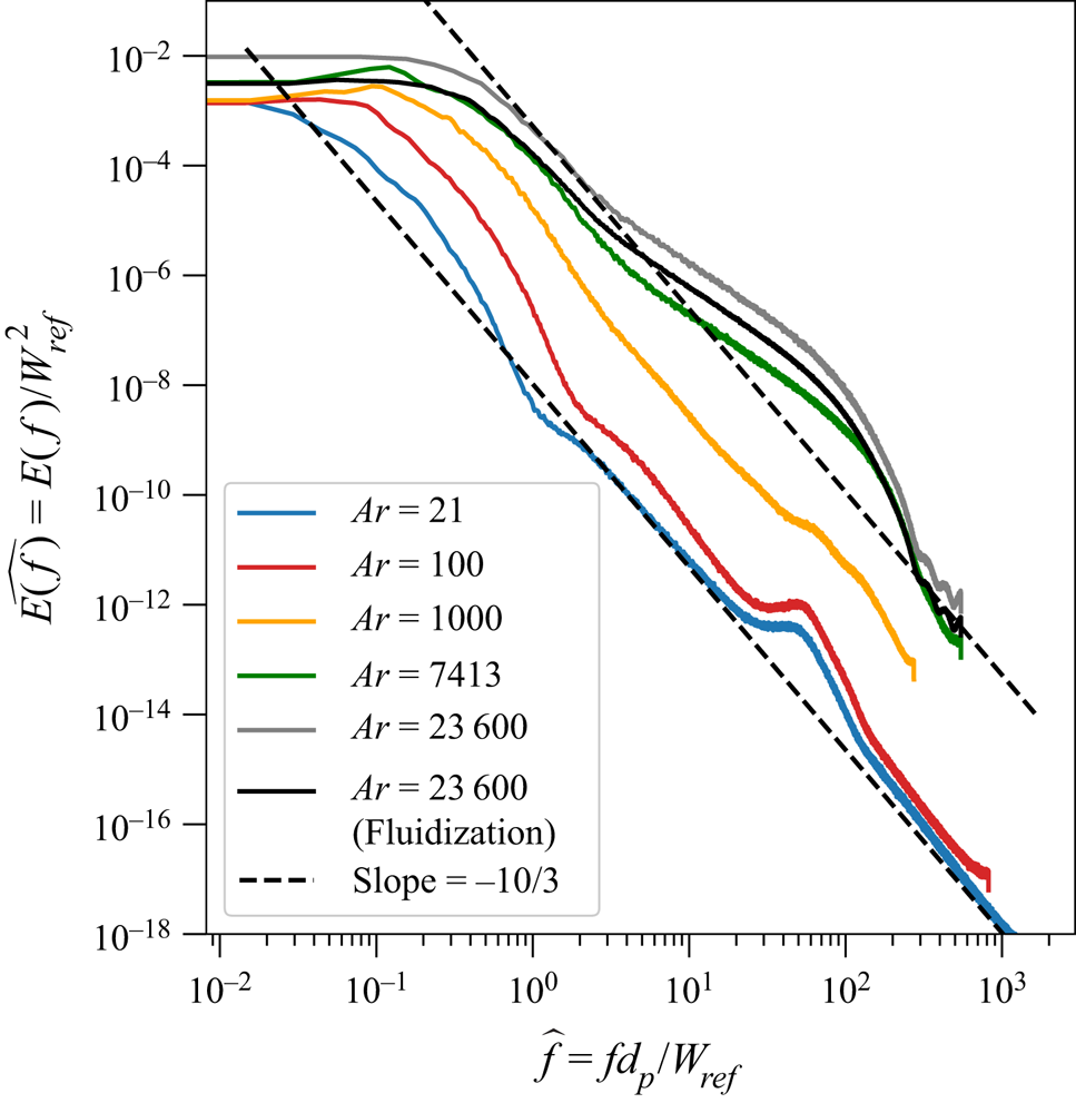
Figure 9 shows the normalized frequency spectra with different  $Ar$ for
 $\phi =0.23$. Similar trends are observed for
 $\phi = 0.30$ and
 $0.43$ (not shown). We also include the simulation of a fluidized bed with
 $Ar = 23\,600$ to demonstrate the independence of domain size. Details of this set-up can be found in the Appendix. The trends of these two cases with
 $Ar=23\,600$ are almost identical except for the magnitude of the spectra even though the length of the fluidized bed (solid black line) is five times higher than the length of the domain in this paper, hence indicating that the spectra are weakly dependent on the domain size.
Normalized frequency spectra  $\widehat {E(\,f)}$ as a function of normalized vertical particle velocity fluctuation frequency
 $\hat {f}$ for different
 $Ar$ and
 $\phi = 0.23$.

The spectra for all values of  $Ar$ are approximately constant at low frequencies. The range of frequencies for constant spectra is proportional to
 $Ar$ while the magnitude of the constant spectra is inversely proportional to
 $Ar$. Both observations are likely due to the dependence of the terminal velocity
 $U_t$ on
 $Ar$. The magnitude of particle velocity fluctuations increases with increasing
 $Ar$ resulting in greater constant spectrum magnitudes. As the terminal velocity increases with increasing
 $Ar$, the normalized domain frequency
 $\hat {f}_{res} = U_t d_p/L w_{ref}$ also increases, resulting in a wider frequency range for constant spectra. Eventually, the spectra decrease and diverge from one another when
 $\hat {f}_t \geqslant \hat {f}_{res}$ following an approximate
 $-10/3$ slope for all
 $Ar$ cases, indicating a power-law relation between the spectra and frequencies.
Spectral slopes have been discussed in the context of Eulerian velocity fluctuations in bubbly flows, for which slopes ranging from  $-8/3$ to
 $-3$ have been found (Lance & Bataille Reference Lance and Bataille1991; Rensen, Luther & Lohse Reference Rensen, Luther and Lohse2005; Riboux, Risso & Legendre Reference Riboux, Risso and Legendre2010; Lai & Socolofsky Reference Lai and Socolofsky2019; Bordoloi et al. Reference Bordoloi, Lai, Clark, Carrillo and Variano2020), and in gas–solid fluidized beds, for which the spectral slopes of pressure fluctuations range from
 $-4$ to
 $-2$ (Johnsson et al. Reference Johnsson, Zijerveld, Schouten, van den Bleek and Leckner2000; van Ommen et al. Reference van Ommen, Sasic, van der Schaaf, Gheorghiu, Johnsson and Coppens2011; van der Schaaf et al. Reference van der Schaaf, Schouten, Johnsson and van den Bleek2002). While the slope of
 $-10/3$ in our simulations is in the range of spectral slopes in the literature, at this time we do not have a physical explanation for this slope given that it represents the Lagrangian particle velocity fluctuations and there are distinct differences between the physical properties of our flow and those that have been published. Nevertheless, it is instructive to compare the spectra from the simulations with this seemingly universal slope of
 $-10/3$ in order to understand how the spectra are modified by clustering. Specifically, when we compare the simulated spectra in figure 9 with the
 $-10/3$ slope (black dashed line), two humps are identified for low
 $Ar$ cases (
 $Ar=21 - 1000$) while only one hump exists for high
 $Ar$ cases (
 $Ar > 1000$). The frequency range of the low-frequency hump decreases as
 $Ar$ increases while the frequency range of the high-frequency hump increases as
 $Ar$ increases. Each hump in the spectrum can be interpreted as an accumulation of energy due to frequent particle velocity fluctuations, indicating dominant time scales or frequencies. We hypothesize that these two time scales or frequencies are associated with short- and long-lived clusters. It is likely that the low
 $Ar$ cases are dominated by long-lived clusters given the larger magnitude of the spectra while the high
 $Ar$ cases are dominated by short-lived clusters (detailed discussion in § 3.5). Hence, these long-lived clusters behave as a single, larger particle and induce stronger velocity fluctuations (Nicolai et al. Reference Nicolai, Herzhaft, Hinch, Oger and Guazzelli1995).
3.4. The effects of Archimedes number on the lifespan and tendency of clustering
To establish a link between the humps observed in the frequency spectra and particle clustering, Voronoï tessellation is used to directly quantify the lifespan and frequency of clusters. In Voronoï tessellation, the domain is decomposed into Voronoï cells in which the centroid of each cell coincides with the centre of a particle. By definition, all points within a Voronoï cell are closer to the centroid of that cell than any other cell. One advantage of the Voronoï tessellation is that an a priori length scale is not required, thus reducing the ambiguity in the analysis. Following Uhlmann & Doychev (Reference Uhlmann and Doychev2014), we define the approximate probability density function (p.d.f.) of quantities associated with randomly arranged particles (Ferenc & Néda Reference Ferenc and Néda2007) as
 \begin{equation} f_d(\boldsymbol{X}) = \dfrac{\left((3d+1)/2\right)^{(3d+1)/2}}{\boldsymbol{\varGamma} \left((3d+1)/2\right)}\boldsymbol{X}^{(3d-1)/2}\exp\left(-\dfrac{3d+1}{2}\boldsymbol{X}\right), \end{equation}
where  $\boldsymbol {X}$ is the random variable representing either the instantaneous Voronoï volume or aspect ratio,
 $d=3$ is the dimension of the Voronoï tessellation and
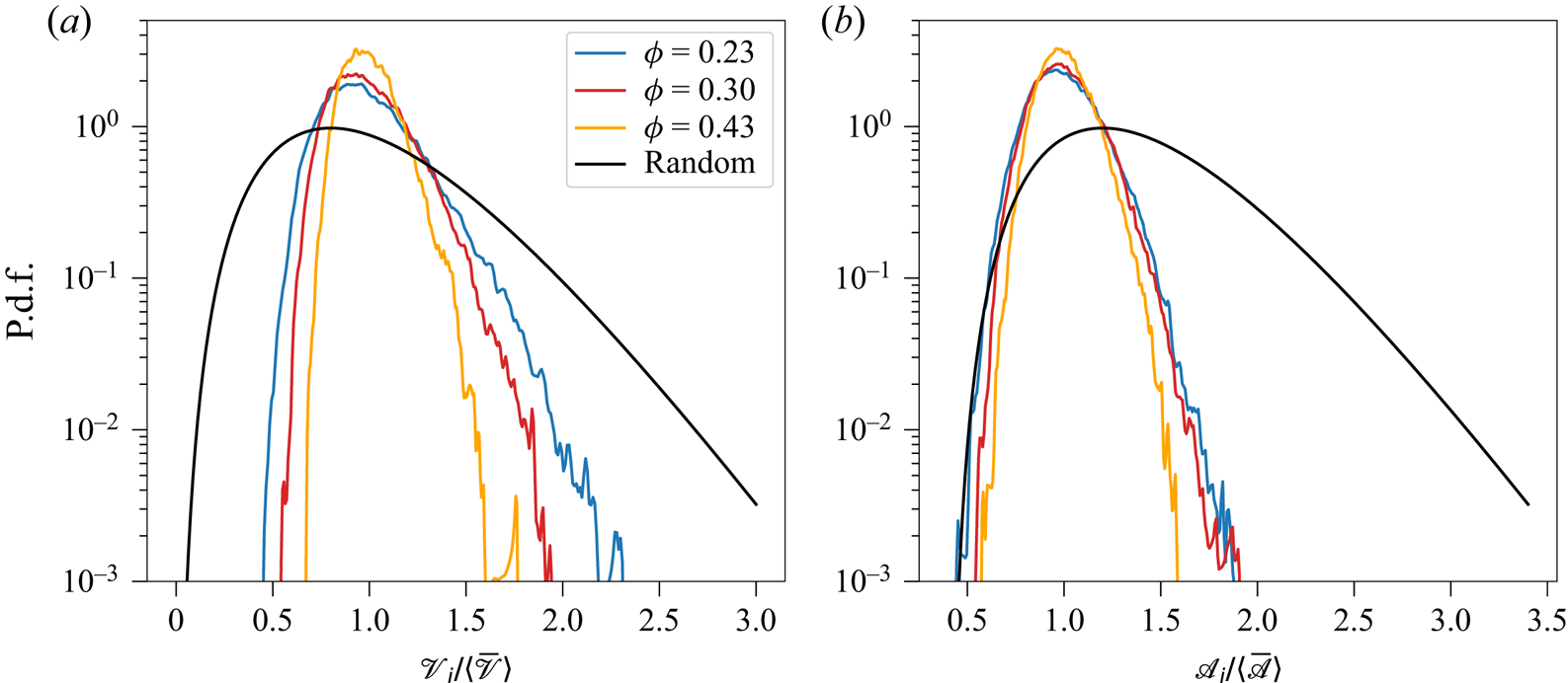
 $\boldsymbol {\varGamma {}}$ is the gamma function. Figure 10(a) shows the distribution of instantaneous Voronoï volumes
 $\mathscr {V}$ normalized by the ensemble- and time-averaged Voronoï volume
 $\langle \bar {\mathscr {V}} \rangle$ for different
 $\phi$ with
 $Ar=21$. Compared with the distribution of randomly arranged particles
 $f_d(\boldsymbol {\mathscr {V}})$, an increase in
 $\phi$ results in a decrease in the width of the p.d.f., indicating a more ordered arrangement. Comparison with different
 $Ar$ for the same
 $\phi$ shows that the effect of
 $Ar$ (not shown) is negligible, indicating that the distribution of instantaneous
 $\mathscr {V}/\langle \bar {\mathscr {V}} \rangle$ depends primarily on
 $\phi$. We analysed the geometry of the Voronoï cells by computing the instantaneous aspect ratio of the
 $i$th Voronoï cell
 \begin{equation} \mathscr{A}_i = \dfrac{\max(\ell_{x,i}, \ell_{y,i})}{\ell_{z,i}}, \end{equation}
where  $\ell _{x,i}$,
 $\ell _{y,i}$ and
 $\ell _{z,i}$ are the largest separation distances between two vertices in the respective
 $x$-,
 $y$- and
 $z$-directions. Figure 10(b) compares the p.d.f. of
 $\mathscr {A}_i$ for the cases in this work with the expected p.d.f. from a random arrangement. The probability of observing large
 $\mathscr {A}_i$ decreases as
 $\phi$ increases, indicating a more ordered arrangement due to squeezed/elongated Voronoï cells. This indicates that the particles prefer a vertical arrangement over a horizontal arrangement because of shielding by the upstream particles which reduces the hydrodynamic forces experienced by the downstream particles. However, in the horizontal direction, the shielding effect from the upstream particles is much weaker because the direction of the flow is perpendicular to the arrangement, hence particles are less likely to be aligned horizontally. The vertical-alignment preferences have been observed in all cases simulated which suggests that instantaneous vertical alignment does not induce observable effects on the hindered settling velocity.
Probability density function of (a) normalized Voronoï volume  $\mathscr {V}_i/\langle \bar {\mathscr {V}} \rangle$ and (b) normalized Voronoï aspect ratio
 $\mathscr {A}_i/\langle \bar {\mathscr {A}} \rangle$ as a function of
 $\phi$ for
 $Ar=21$.

To quantify temporal effects, we compute the clustering frequency and lifespan. A cluster is defined as a Voronoï volume satisfying  $\mathscr {V}_i < \mathscr {V}_{c,{lower}}$ and voids as
 $\mathscr {V}_i > \mathscr {V}_{c,{upper}}$ where
 $\mathscr {V}_{c,{lower}}$ and
 $\mathscr {V}_{c,{upper}}$ are the lower and upper bounds defined by the intersection of the simulated p.d.f.s with the randomly arranged p.d.f. given by (3.7). Qualitatively, all simulated cases contain significant numbers of clusters and voids, although more quantitative aspects of clusters concern their lifespan and frequency. More frequent, long-lived clusters can induce appreciable acceleration because clusters can behave as a particle with large inertial effects. To compare the lifespan of clusters across the range of simulated
 $Ar$, we utilized the reference time scale
 $t_{ref} = d_p/w_{ref}$ and computed a clustering frequency

where  $\widehat {\mathscr {V}_i}^{t}$ is the normalized Voronoï volume at time
 $t$ and
 is the indicator function

As such,  when a particle leaves the cluster,
 $0$ when a particle neither enters nor leaves the cluster and
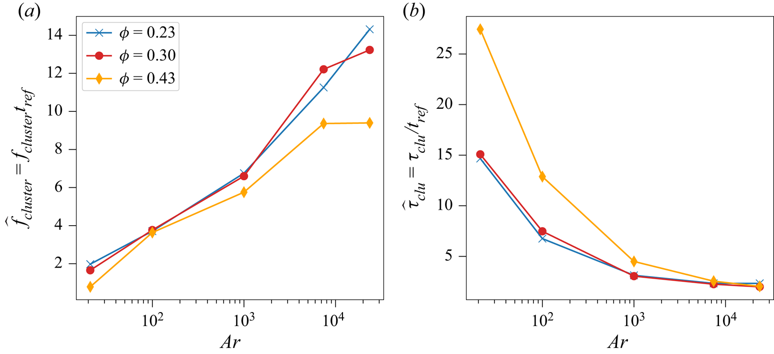
 $-1$ when it enters the cluster. Figure 11(a) shows the normalized clustering frequency
 $\hat {f}_{cluster} = \,f_{cluster}t_{ref}$ as a function of
 $Ar$. Comparing cases with the same
 $\phi$, as
 $Ar$ increases,
 $\hat {f}_{cluster}$ also increases probably because strong velocity fluctuations at higher
 $Ar$ increase the probability of particles coming into contact with one another (Uhlmann & Doychev Reference Uhlmann and Doychev2014), resulting in more clusters. For cases with the same
 $Ar$, as
 $\phi$ increases, the normalized clustering frequency decreases because more frequent collisions are likely to break apart clusters. Defining the lifespan of clusters as

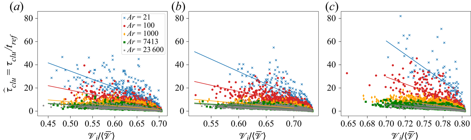
figure 11(b) shows the normalized average cluster lifespan  $\hat {\tau }_{{clu}} = \tau _{{clu}}/t_{ref}$ as a function of
 $Ar$ and shows that as
 $Ar$ increases,
 $\hat {\tau }_{{clu}}$ significantly decreases. This is probably due to collisions that break apart clusters. Interestingly, taking the inverse of
 $\hat {\tau }_{clu}$ gives a normalized frequency that falls into the middle of the low-frequency hump for low
 $Ar$ cases (
 $Ar=21 - 1000$) and tail of high-frequency hump for high
 $Ar$ cases in figure 9. This again suggests the humps are due to the particle velocity fluctuations induced by both short- and long-lived clusters. Figure 12 shows the relationship between the normalized Voronoï volumes and the normalized lifespan of clusters. As
 $Ar$ increases, the slope of dependence decreases drastically, indicating weaker dependence of the lifespan on the Voronoï volumes. As
 $\phi$ increases, the dependence of the cluster lifespan on the normalized volumes also increases. Combining the results from the normalized lifespan of clusters and clustering frequency, we show that as
 $Ar$ increases, the decreased cluster lifespan is accompanied by a significant increase in the clustering frequency which indicates that low
 $Ar$ is characterized by fewer but longer-lived clusters while high
 $Ar$ is characterized by more short-lived clusters. Overall, due to a significant number of long-lived clusters in low-
 $Ar$ particle suspensions, an appreciable increase in the hindered settling velocity is observed, hence resulting in higher
 $k$. In contrast, in high-
 $Ar$ particle suspensions, a large number of short-lived clusters is insufficient to induce appreciable particle acceleration, leading to a lower
 $k$.
(a) Clustering frequency  $f_{cluster}$ and (b) normalized cluster lifespan
 $\tau _{{clu}}/t_{ref}$ as a function of
 $Ar$ for different
 $\phi$.

Normalized cluster lifespan  $\tau _{{clu}}/t_{ref}$ as a function of normalized Voronoï volume
 $\mathscr {V}_i/\langle \overline {\mathscr {V}} \rangle$ for different
 $Ar$ and
 $\phi$: (a)
 $\phi = 0.23$, (b)
 $\phi = 0.3$ and (c)
 $\phi = 0.43$.

3.5. Effect of collisions and hydrodynamic forces on clustering
In a concentrated suspension, there are two primary types of interactions, namely fluid–particle interactions induced by hydrodynamic forces and particle–particle interactions induced by collisions. As shown by Esteghamatian et al. (Reference Esteghamatian, Hammouti, Lance and Wachs2017), the primary role of collisions in concentrated suspensions is to transfer momentum from the axial direction to the transverse direction and induce stronger velocity fluctuations in the transverse directions.
Following Esteghamatian et al. (Reference Esteghamatian, Hammouti, Lance and Wachs2017) and Nicolai et al. (Reference Nicolai, Herzhaft, Hinch, Oger and Guazzelli1995), we computed the autocorrelation of the instantaneous particle velocity fluctuation as
 \begin{equation} R_{U_iU_i}(\tau) = \langle U^\prime_{i,n}(t_0)U^\prime_{i,n}(t_0 + \tau) \rangle \end{equation}
along with the normalized value
 \begin{equation} \widehat{R_{U_iU_i}}(\tau) = \dfrac{R_{U_iU_i}(\tau)}{\langle U^\prime_{i,n}(t_0)U^\prime_{i,n}(t_0) \rangle}, \end{equation}
where the fluctuating particle velocity of particle  $n=1,\ldots,N_p$ is defined as
 $U^\prime _{i,n} = U_{i,n} - \langle \bar {U}\rangle _i$,
 $t_0$ is a chosen time and
 $i=x$,
 $y$ or
 $z$. Here, the overbar is the time-averaging operator defined in (2.5) and the angle bracket
 $\langle \cdot \rangle$ indicates an ensemble average over all particles. The autocorrelation time scale of the velocity fluctuations is given by
 \begin{equation} \mathcal{T}_i = \lim_{\tau\rightarrow \infty} \int \widehat{R_{U_iU_i}}(\tau) \,\textrm{d}\tau \end{equation}
and the self-diffusivity is
 \begin{equation} \mathcal{D}_i = \lim_{\tau\rightarrow \infty} \int R_{U_iU_i}(\tau) \,\textrm{d} \tau, \end{equation}
where  $i=x$,
 $y$ or
 $z$.
To quantify the effects of collisions, time- and ensemble-averaged effective collision frequency  $\langle \overline {f_c} \rangle _{eff}$ are computed. A collision between two particles occurs when the separation distance between the particles’ centres is less than the particle diameter
 $d_p$. As a result, the collision frequency is a monotonically decreasing function of the volume fraction because the likelihood of a collision decreases as the mean separation distance between particles increases. However, this approach leads to overestimation of effective collisions (Ozel et al. Reference Ozel, Brändle de Motta, Abbas, Fede, Masbernat, Vincent, Estivalezes and Simonin2017). Restricting collisions to those with appreciable normal contact velocities is achieved by defining the collision Stokes number
 \begin{equation} St_{imp} = \dfrac{U_{imp}\rho_p d_p}{9\rho_f \nu_f}, \end{equation}
where  $U_{imp}$ is the normal component of the relative particle velocities contacting one another. If the number of times a particle
 $n$ collides with another particle during a simulation time step
 $n_t$ with
 $St_{imp} > St_{thresh}$ (where
 $St_{thresh}$ is the threshold Stokes number, defined below) is given by
 $\tilde {N}_{c,n}^{n_t}$, then the time- and ensemble-averaged collision frequency is given by
 \begin{equation} \langle \overline{f_c} \rangle_{eff} = \frac{1}{N_p(t_{max}-t_0)}\sum_{l=n_{t,0}}^{n_{t,max}}\sum_{n = 1}^{N_p} \tilde{N}_{c,n}^{l}, \end{equation}
where  $n_{t,0}=t_0/\Delta t$ and
 $n_{t,max}=t_{max}/\Delta t$.
The threshold Stokes number is then determined by computing a threshold collision velocity with an empirical function relating the restitution coefficient to the Stokes number. If the vertical velocity of a particle before being subject to lubrication and contact forces is  $U_{t,0}$, then the restitution coefficient is given by as
 \begin{equation} \varepsilon = \dfrac{U_{r}}{U_{t,0}} = \varepsilon_{max} \exp\left(-\dfrac{30}{St_{0}}\right), \end{equation}
where  $U_r$ is the rebound velocity of a particle after collision and
 $\varepsilon _{max} \approx 0.91$ is the maximum restitution coefficient when
 $St_{0} \rightarrow \infty$, and
 \begin{equation} St_{0} = \dfrac{U_{t,0}d_p \rho_p}{9\rho_f \nu_f} \end{equation}
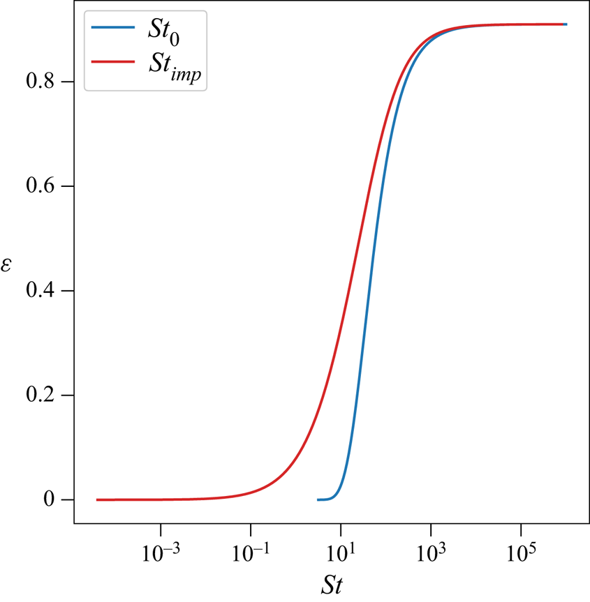
is the Stokes number based on  $U_{t,0}$. Figure 13 shows the effect of
 $St_{0}$ on
 $\epsilon$, demonstrating that a collision is only effective when an appreciable
 $U_{r}$ can be achieved for
 $\epsilon > 0$. We rearranged (3.18) to relate
 $St_{imp}$ to
 $\epsilon$ by using the dry restitution coefficient
 $e_{dry} = U_{r}/U_{imp}$ such that
 \begin{equation} St_{imp} = \dfrac{30\varepsilon}{e_{dry} (\log \varepsilon - \log \varepsilon_{max})}, \end{equation}
where  $U_{imp}$ is the precollision impact velocity. Figure 13 shows the effect of
 $St_{imp}$ on
 $\epsilon$. In this paper, we define
 $St_{thresh} = 0.22$ as the Stokes number at which
 $\varepsilon = 0.025$, which represents the value of
 $\epsilon$ at which
 $St_{imp}$ is exceeded by 95 % of all values of
 $St_{imp}$ in figure 13.
The restitution coefficient  $\epsilon$ as a function of
 $St_0$ and
 $St_{imp}$.

To compare the effects of hydrodynamic and collision forces, we computed the ratio of the hydrodynamic fluctuation length scale to the mean free path between collisions  $\lambda _{hydro, i}/\lambda _{col,i}$, where
 $$\begin{gather} \lambda_{hydro, i} = \sqrt{\mathcal{D}_i \mathcal{T}_i}, \end{gather}$$
 $$\begin{gather}\lambda_{col,i} = \sqrt{\mathcal{D}_i/\langle \overline{f_c} \rangle_{eff}}, \end{gather}$$
where  $i = x$,
 $y$ and
 $z$. The mean free path between collisions,
 $\lambda _{col,i}$, quantifies the average distance the particles travel between collisions, while the hydrodynamic fluctuation length scale,
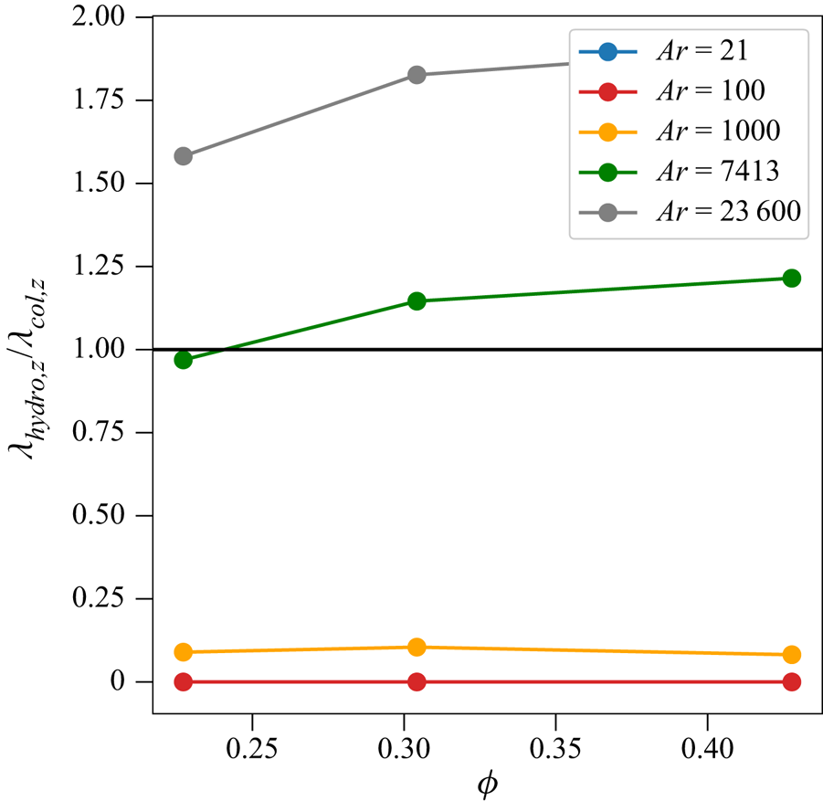
 $\lambda _{hydro, i}$, measures the distance over which the particle velocity fluctuations are still correlated. Figure 14 shows the ratio
 $\lambda _{hydro,z}/\lambda _{col,z}$ that quantifies the relative effects of hydrodynamic to collision forces. Similar trends are observed for the
 $x$- and
 $y$-direction (not shown). Since
 $\lambda _{hydro,z}/\lambda _{col,z} \approx 0$ for
 $Ar = 21$ and
 $100$, the mean free path is close to infinitely large, indicating a dominance of hydrodynamic forces without effective particle–particle collisions. Since
 $0 \leqslant \lambda _{hydro,z}/\lambda _{col,z} \ll 1$ for
 $Ar = 1000$, the mean free path is much larger than the hydrodynamic fluctuation length scale, still allowing particles to be influenced by appreciable hydrodynamic forces with few particle–particle collisions. Since
 $\lambda _{hydro,z}/\lambda _{col,z} \geqslant 1$ for
 $Ar = 7413$ and 23 600, the mean free path is shorter than the hydrodynamic fluctuation length scale, indicating a dominance of particle collisions, hence particles collide before experiencing appreciable wake interactions induced by hydrodynamic fluctuations. In general, as
 $Ar$ increases,
 $\lambda _{hydro,z}/\lambda _{col,z}$ increases significantly indicating
 $\lambda _{col,z}$ decreases at a rate much faster than the decrease in
 $\lambda _{hydro,z}$. As a result, the effects of collisions are more significant and dominate over the hydrodynamic forces for high
 $Ar$ cases, preventing particles from experiencing appreciable wake interactions. Similarly,
 $\lambda _{hydro,z}/\lambda _{col,z}$ increases slightly with an increase in
 $\phi$, indicating a weak dependence on the volume fraction. As reported by Uhlmann & Doychev (Reference Uhlmann and Doychev2014), particles cluster and accelerate when they experience appreciable fluctuations induced by wake interactions or the ‘drafting–kissing–tumbling’ effect from interacting particles. In our simulations, particles tend to cluster because of the particle velocity fluctuations and wake interactions at all values of
 $Ar$. However, for low
 $Ar$ cases, clusters are less likely to break up because of insignificant collisions, resulting in long-lived clusters and higher hindered settling or a larger value of
 $k$. For high
 $Ar$ cases, clusters are likely to break up because of strong collisions, leading to short-lived clusters, therefore lower hindered settling and a smaller value of
 $k$.
The ratio of vertical hydrodynamic fluctuation length scale  $\lambda _{hydro, z}$ to the vertical mean free path between collisions
 $\lambda _{col,z}$ as a function of volume fraction
 $\phi$ for different
 $Ar$.

4. Summary and conclusion
We studied the effects of particle properties on the hindered settling velocity in PRS simulations of three-dimensional, triply periodic, monodispersed particle suspensions. The primary parameter of interest is the Archimedes number  $Ar$ which is varied by varying the fluid kinematic viscosity
 $\nu _f$ and particle-fluid density ratio
 $s$. Analysis of various statistics provided insights into the effects of particle clustering on hindered settling. By plotting the prefactor
 $k$ obtained from the literature over our simulation results as a function of
 $Ar$, we demonstrate that
 $k$ converges to 0.89 for concentrated suspension as
 $Ar \rightarrow 0$ and decreases as
 $Ar$ increases according to an exponential function (3.4), indicating smaller hindered settling for high
 $Ar$. We found that the normalized particle velocity fluctuation variance decreases as
 $Ar$ increases, indicating that particles experience less wake interactions and less ‘drafting-kissing-tumbling’ effects. Frequency spectra demonstrated two humps at low and high frequency for low
 $Ar$ and one hump at high frequency for high
 $Ar$. These humps indicate an accumulation of energy and are likely due to the existence of two types of short- and long-lived particle clusters.
To understand the existence of clustering, we employed Voronoï tessellation to compute the simulated p.d.f. of normalized Voronoï volumes. By comparing the simulated p.d.f. with the p.d.f. of randomly arranged particles, we found that both short- and long-lived clusters exist for all  $Ar$ cases with different volume fractions
 $\phi$ with the particles favouring vertical alignment, leading to a reduced instantaneous aspect ratio of the normalized Voronoï volumes. The simulated p.d.f.s also suggest that
 $\phi$ has stronger effects on the particle arrangement as compared with
 $Ar$ which more strongly affects particle clustering. By analysing the normalized lifespan and normalized frequency of clusters, we show that the normalized lifespan of clusters decreases with increasing
 $Ar$ and decreasing
 $\phi$ while the normalized frequency of clusters increases with increasing
 $Ar$ and decreasing
 $\phi$. Both the normalized lifespan and normalized frequency strongly depend on
 $Ar$ and weakly on
 $\phi$. By analysing the normalized lifespan of clusters as a function of the normalized Voronoï volume, we found that large clusters have longer lifespans for all
 $Ar$ cases, although the increase in the lifespan is much higher for low
 $Ar$ cases. Furthermore, the inverses of the cluster lifespans for all
 $Ar$ cases fall within the dominant humps in the corresponding frequency spectra which indicates energy accumulation is indeed due to particle clustering. This shows that low
 $Ar$ and high
 $\phi$ cases are characterized by less frequent and long-lived clusters while high
 $Ar$ and low
 $\phi$ cases are characterized by more frequent, short-lived clusters.
By quantifying the effects of hydrodynamic forces relative to collision forces with the ratio of the mean free path between collisions  $\lambda _{col,z}$ to the hydrodynamic fluctuation length scale
 $\lambda _{hydro,z}$, we showed that the effects of collisions increase at a rate much faster than the increase in the effects of hydrodynamic fluctuations with increasing
 $Ar$, while the effect of
 $\phi$ was weak. For
 $Ar = 21$ and
 $100$,
 $\lambda _{hydro,z}/\lambda _{col,z} \approx 0$, indicating that collisions are insignificant and particles can freely experience wake interactions and ‘drafting–kissing–tumbling’ effects, resulting in higher hindered settling and a value of
 $k$. When
 $Ar = 1000$,
 $0 < \lambda _{hydro,z}/\lambda _{col,z} \ll 1$, the effects of collisions become stronger although particles still experience appreciable wake interactions with less frequent collisions. When
 $Ar = 7413$ and 23 600,
 $\lambda _{hydro,z}/\lambda _{col,z} > 1$, indicating that the effects of collisions dominate over the hydrodynamic fluctuations. The particles in this regime rarely experience wake interactions because of frequent collisions, resulting in lower hindered settling and a lower value of
 $k$.
In application of fluidized-bed reactors for wastewater treatment, flow short circuiting should be minimized to ensure maximum utilization of particle surfaces for optimal microbial growth and biological degradation. Our results imply that flow short circuiting within fluidized bed reactors is likely to occur when clustering is long-lived. Therefore, our results suggest that operating fluidized-bed reactors in a regime that has short-lived clusters, or with particles having  $Ar > 1000$ is likely to reduce flow short circuiting. Though experimental validation of fluidized-bed reactors is needed, previous fluidized bed reactor studies have demonstrated that satisfactory treatment performance is achieved when
 $Ar = 2000 - 20\,000$ (Shin et al. Reference Shin, McCarty, Kim and Bae2014). We anticipate that the results of this study will inform fluidized-bed reactor design for domestic and industrial wastewater treatment based on
 $Ar$, enabling more reliable and energy-efficient operation.
Funding
This work was funded by the California Energy Commission (CEC) under CEC project number EPC-16-017, the US NSF Engineering Center for Reinventing of the Nation's Urban Water Infrastructure (ReNUWIt) under award no. 1028968 and Office of Naval Research Grant N00014-16-1-2256. Simulations were conducted with supercomputer resources under XSEDE Project CTS190063. We thank H. Lee and S. Balachandar from the University of Florida for providing us with their IBM code. We also thank E. Biegert, B. Vowinckel, T. Köllner and E. Meiburg from the University of California, Santa Barbara, for assistance with implementation of the collision models. This document was prepared as a result of work sponsored in part by the California Energy Commission. It does not necessarily represent the views of the Energy Commission, its employees, or the State of California. Neither the Commission, the State of California, nor the Commission's employees, contractors, or subcontractors makes any warranty, express or implied, or assumes any legal liability for the information in this document; nor does any party represent that the use of this information will not infringe upon privately owned rights. This document has not been approved or disapproved by the Commission, nor has the Commission passed upon the accuracy of the information in this document.
Declaration of interests
The authors report no conflict of interest.
Appendix. Simulation set-up of a fluidized bed
For the simulation of a fluidized bed, three-dimensional simulations are conducted with  $N_p=2000$ particles in a rectangular domain. The particles have an Archimedes number
 $Ar=23\,600$. The grid spacing is uniform in the
 $x$-,
 $y$- and
 $z$-directions and the grid resolution is given by
 $\Delta x= \Delta y = \Delta z=h=d_p/25.6$. The rectangular domain has cross-sectional dimension
 $L_x = L_y = 10 d_p$ and its length is
 $L_z = 60 d_p$ with
 $256\times 256 \times 1536$ grid points. The time-step size is
 $\Delta {t}=1.5\times 10^{-4}$ s, resulting in a maximum advection Courant number of
 $0.5$ for the six cases simulated. The cases are run with periodicity in the
 $x$- and
 $y$-directions. The pressure is specified at the top boundary as
 $p=0$, while at the bottom boundary the inflow velocity is specified as uniform and given by
 $\tilde {U}$. The primary parameter of interest is the particle Reynolds number
 $Re_p = \tilde {U} d_p/\nu _f$, where the average upflow velocity at the inlet,
 $\tilde {U}$, is varied to investigate Reynolds number effects. A total of six simulations were conducted with
 $0.010\leqslant \tilde {U} \leqslant 0.035$, giving
 $20 \leqslant Re_p \leqslant 70$.