1. Introduction
Fluid–structure interaction (FSI) is a pervasive phenomenon in both natural and engineered systems, where the interplay between fluid forces and structural response drives complex and often nonlinear dynamics. It underpins critical processes in fields ranging from aerospace and energy systems to biofluid mechanics. Typical examples include wing flutter, vortex-induced vibration (VIV) of marine risers, turbine blade responses, wind-induced vibrations of bridges and blood–artery interactions. In FSI systems, fluid flow can induce structural deformation or vibration, while the resulting structural motion in turn modifies the surrounding flow field. Moreover, FSI inherently spans multiple temporal and spatial scales, from local transient vortices to global structural dynamics. Its key characteristics – strong nonlinearity, multiphysics coupling and multiscale behaviour – render the analysis and prediction of FSI particularly challenging, motivating the need for systematic studies of underlying mechanisms and dynamical responses.
Early investigations primarily focused on two-dimensional (2-D) structures. Pioneering wind tunnel experiments by Feng (Reference Dowell and Hall1968) examined the transverse vibrations of cylinders, demonstrating that lock-in arises when the vortex-shedding frequency approaches the structure’s natural frequency, resulting in amplified vibration amplitudes. In a systematic study of VIV on cylinders with low mass ratios, Williamson & Roshko (Reference Williamson and Govardhan1988) were the first to identify that the amplitude response curve exhibits two distinct branches. They further classified wake vortex-shedding patterns into multiple modes, including ‘2S’, ‘2P’, ‘P+S’ and ‘2T’. Subsequent empirical studies (Sarpkaya Reference Raza, Chern, Susanto and Zhou1979; Gharib Reference Flinois and Morgans1999; Govardhan & Williamson Reference Goldstein, Handler and Sirovich2000) have investigated single-degree-of-freedom (single-DOF) VIV in the transverse direction, analysing how Reynolds number, mass ratio and damping affect vibration amplitude, frequency and phase. Additionally, Bearman (Reference Balajewicz and Dowell1984), Naudascher & Rockwell (Reference Li, Lyu, Kou and Zhang1980) and Sumer (Reference Schmid2006) provided extensive characterisations of single-DOF VIV features. Collectively, these studies laid a solid foundation for understanding the fundamental mechanisms governing vortex-induced vibrations.
As three-dimensional (3-D) models more accurately represent real-world conditions, research attention has gradually shifted towards 3-D bluff bodies. Among them, the sphere – a fundamental and widely studied geometry – was an early focus. Johnson & Patel (Reference Jiang, Pfister, Huang and Cao1999) conducted numerical and experimental investigations on a stationary sphere. His simulations enabled systematic analysis of flow instabilities across Reynolds numbers, with results validated against experiments, establishing a solid foundation for subsequent studies of 3-D sphere flow instabilities. A decade later, Giacobello, Ooi & Balachandar (Reference Gharib2009) examined the wake of a sphere rotating steadily about its transverse axis in uniform flow, using a highly accurate Fourier–Chebyshev spectral collocation method. His findings elucidated how rotation influences wake vortex structures and hydrodynamic forces on the sphere.
Numerical studies of flow-induced vibration (FIV) for 3-D spheres emerged in 2011. Behara, Borazjani & Sotiropoulos (Reference Bearman2011) investigated the FIV response of an elastically mounted sphere at
 ${\textit{Re}} = 300$
with mass ratio
 $m^* = 2$
, allowing oscillations in all three directions. The study quantified variations in vibration amplitude, frequency and hydrodynamic force coefficients, identifying two distinct vortex-shedding modes – hairpin and spiral – associated with hysteresis phenomena. In the hairpin mode, the sphere oscillates along a straight transverse trajectory, whereas in the spiral mode, it follows a circular orbit, yielding larger amplitudes. Subsequently, Lee, Hourigan & Thompson (Reference Kutz, Brunton, Brunton and Proctor2013) investigated the flow modes of a tethered sphere using a spectral-element-Fourier method. Across a Reynolds number range of 50–12 000, seven distinct flow regimes were identified for a neutrally buoyant tethered sphere, each characterised by unique mean inclination angles, vibration amplitudes, frequencies and cross-flow trajectories. The effect of Reynolds number on vibration behaviour was systematically analysed, revealing motion evolution from linear oscillations to chaotic vibrations and eventually to quasi-circular orbits with increasing
 $Re$
, accompanied by a transition in wake structures from symmetric double-threaded patterns to irregular vortex shedding. Building on this, Behara & Sotiropoulos (Reference Behara, Borazjani and Sotiropoulos2016) extended numerical studies of 3-D sphere FIV across
 $Re$
= 300–1000, analysing responses across vibration modes with a focus on amplitude, frequency and trajectory. The Reynolds number strongly influenced wake dynamics and motion trajectories, with
 ${\textit{Re}} = 500$
showing a clear transition from circular to elliptical orbits. Since 2018, Rajamuni and colleagues have systematically advanced the understanding of 3-D sphere flow-induced vibrations. Their studies examined transverse FIV, rotational effects and the influence of degrees of freedom on amplitude, frequency, wake structures and phase (Rajamuni et al. Reference Rajamuni, Hourigan and Thompson2018a
,
Reference Rajamuni, Thompson and Houriganb
, Reference Rajamuni, Thompson and Hourigan2019). Notably, they demonstrated how rotation and 3-DOF motion modulate vibration amplitude, alter wake topology and modify synchronisation ranges, while dynamic mode decomposition revealed periodic wake features across different regimes. Collectively, these works elucidate the coupled mechanisms underlying 3-D sphere FIV, revealing the rich and intricate dynamics of what might superficially appear as a simple system.
As research has deepened, attention has increasingly turned to the FIV of spheres under more complex conditions, including near free surfaces (Rajamuni, Hourigan & Thompson Reference Rai and Moin2021; Chizfahm, Joshi & Jaiman Reference Chizfahm and Jaiman2021), under external magnetic fields (Yao et al. Reference Yao, Jia, Zhang and Gui2023b ) and in multi-sphere configurations (Raza et al. Reference Rajamuni, Thompson and Hourigan2020). These studies have provided valuable insights into the nonlinear dynamics of spheres in such complex environments, further enriching the understanding of their behaviour.
To unravel the underlying stability mechanisms of FSI while alleviating the high computational cost of full-order simulations, reduced-order models (ROMs) have emerged as a powerful tool. In particular, the eigensystem realisation algorithm (ERA) has proven highly effective in extracting linear stability characteristics from nonlinear impulse responses (Flinois & Morgans Reference Feng2016; Yao & Jaiman Reference Williamson and Roshko2017). By identifying the eigenvalues of coupled wake–structure modes, this method enables a clear distinction between resonance-induced and flutter-induced instabilities. ERA has demonstrated high predictive accuracy for 2-D FIV of rigid bodies (Flinois & Morgans Reference Feng2016; Yao & Jaiman Reference Williamson and Roshko2017; Li et al. Reference Lee, Hourigan and Thompson2019; Yao & Jaiman Reference Yao and Jaiman2019; Bukka, Magee & Jaiman Reference Behara and Sotiropoulos2020; Cheng et al. Reference Bukka, Magee and Jaiman2023), yet its application to 3-D scenarios remains limited. Chizfahm & Jaiman (Reference Chizfahm and Jaiman2021) investigated the vibration behaviour of a canonical 3-D sphere, addressing the gap left by earlier studies focused on 2-D cylinders. Their work systematically analysed frequency-locking phenomena and self-sustained vibration mechanisms, identifying distinct vibration modes and their corresponding reduced-velocity ranges. More recently, Cheng et al. (Reference Cheng, Lien, Dowell, Yee, Wang and Zhang2024) conducted a numerical study of flow-induced vibration in an elastically mounted cube at
 ${\textit{Re}} = 300$
, highlighting asymmetric wake instabilities in two orthogonal transverse directions and their influence on structural responses. The study also compared cube vibration characteristics across different degrees of freedom and examined the role of initial kinetic energy in triggering stability transitions and mode shifts.
Previous research on flow-induced vibrations has primarily focused on classical bodies with perfect geometric symmetry, such as spheres, yet it is well established that geometry plays a crucial role in shaping wake dynamics and vibration responses. For instance, spheres exhibit limited vibration amplitudes in the desynchronised regime at high
 $U_r$
due to drifting vortex shedding planes (Rajamuni et al. Reference Rajamuni, Hourigan and Thompson2018a
), whereas elongated ellipsoids may break this geometric isotropy, stabilising the shedding orientation. In practical applications, most bluff bodies are inherently geometrically asymmetric or anisotropic, and slender ellipsoids may serve as a simplified model to study such effects. This raises key questions: how does the anisotropic geometry of ellipsoids influence vibration dynamics and wake patterns? To date, only a very limited number of experimental studies on spheroid FIV has been reported (Obando et al. Reference Noack, Afanasiev, Morzyński, Tadmor and Thiele2024) and, to our knowledge, no numerical investigations exist.
To address this gap, the present study investigates the 3-D flow-induced vibration of a prolate spheroid with an aspect ratio
 $\epsilon = 3$
using the lattice Boltzmann method (LBM) coupled with an immersed boundary (IB) approach. The effects of reduced velocity and different initial conditions are examined. This study aims to systematically characterise its dynamic responses, identify dominant wake and structural modes, and clarify the role of multi-stability and hysteresis in complex vibration regimes. The remainder of this paper is organised as follows. Section 2 describes the physical model, numerical methods and validation procedures. Section 3 presents a systematic analysis of the results, including the spheroid’s vibration responses, flow-field and wake dynamics, DMD of flow structures, response branches and hysteresis, and linear stability analysis using the ERA-based ROM. Finally, § 4 summarises the main findings and conclusions.
Schematic of the computational domain and physical model. A three-dimensional spheroid with a major axis length of
 $D$
is placed in a uniform inflow
 $U$
. The spheroid is elastically supported by a spring with stiffness
 $k$
and a damper with damping coefficient
 $c$
. The computational domain extends
 $15D$
upstream,
 $35D$
downstream, and
 $30D$
in both the width and height directions.

2. Physical problem and methodology
2.1. Physical model
Figure 1 shows a schematic of a spheroid undergoing flow-induced vibration. In this set-up, the body is modelled as a slender prolate spheroid with polar radius
 $b$
, equatorial radius
 $a$
and mass
 $m$
, elastically mounted in a uniform flow of velocity
 $U$
. The major axis has length
 $D = 2b$
and the aspect ratio is fixed at
 $\epsilon = b/a = 3$
. The support is characterised by a spring of stiffness
 $k$
and a damping coefficient
 $c$
. The spheroid’s motion is restricted to the
 $z$
-direction and governed by fluid–structure interaction, resulting in a single-DOF FIV system.
The fluid flow is governed by incompressible Navier–Stokes equations as follows:
 \begin{align} \boldsymbol{\nabla }\boldsymbol{\cdot }\boldsymbol{u}& = 0, \end{align}
 \begin{align} \rho \left (\frac {\partial \boldsymbol{u}}{\partial t}+\boldsymbol{u} \boldsymbol{\cdot }\boldsymbol{\nabla }\boldsymbol{u}\right )& = -\boldsymbol{\nabla }p+\mu \boldsymbol{\nabla} ^{2} \boldsymbol{u}+\boldsymbol{f}_{\!b}, \end{align}
where the dimensional variables include the fluid velocity
 $\boldsymbol{u}=(u,v,w)$
, the fluid pressure
 $p$
, the fluid density
 $\rho$
and the dynamic viscosity
 $\mu$
. The body force term
 $\boldsymbol{f}_{\!b}$
represents the Eulerian momentum force exerted on the surrounding fluid by the immersed boundary, subject to the no-slip condition on the spheroid surface. A uniform velocity
 $U$
is prescribed at the inlet and the lateral boundaries of the fluid domain, while a constant pressure with
 $\partial \boldsymbol{u}/\partial x = \textbf{0}$
is imposed at the outlet. Initially, the fluid is at rest.
The vibration of an elastically mounted spheroid is a 1-DOF vibration system and can be represented by an equation of motion:
 \begin{equation} m \ddot {\boldsymbol{z}}_{\text{c}}+c \dot {\boldsymbol{z}}_{\text{c}}+k \boldsymbol{z}_{\text{c}}=F_{z}(t), \end{equation}
where
 $m$
denotes the mass of the spheroid,
 $c$
represents the damping coefficient and
 $k$
is the spring constant. Furthermore,
 $\boldsymbol{z}_{\text{c}}$
,
 $\dot {\boldsymbol{z}}_{\text{c}}$
and
 $\ddot {\boldsymbol{z}}_{\text{c}}$
correspond to the displacement, velocity and acceleration of the spheroid along the
 $z$
-axis, respectively. The force
 $ {F_z}{(t)}$
represents the resultant lift acting on the spheroid along the
 $z$
-axis. Initially, the spheroid is stationary, with
 $\boldsymbol{z}_{\text{c}}=0$
,
 $\dot {\boldsymbol{z}}_{\text{c}}=0$
and
 $\ddot {\boldsymbol{z}}_{\text{c}}=0$
at
 $t=0$
.
Equation (2.3) can be normalised by using
 $D$
,
 $U$
and
 $\rho$
as the characteristic quantities,
 \begin{equation} \frac {\text{d}^{2} Z}{\text{d} t^{* 2}}+\frac {4 \pi \zeta }{U_{r}} \frac {\text{d} Z}{\text{d} t^{*}}+\left (\frac {2 \pi }{U_{r}}\right )^{2} Z=\frac { C_{l}}{2 m^{*}}, \end{equation}
where the lift coefficient is defined as
 $C_l = F_{z}/((1/2) \rho U^2 D^2)$
and the non-dimensional transverse displacement of the spheroid is
 $Z = \boldsymbol{z}_c/D$
. The dimensionless time is given by
 $t^* = tU/D$
. To simplify the notation,
 $t$
will represent the dimensionless time for the remainder of this paper.
Key parameters governing the vibration of the spheroid include: the mass ratio
 $m^* = m/m_d$
, with
 $m_d = \rho D^3$
representing the mass of the fluid that is displaced; the damping ratio expressed as
 $\zeta = c/(2\sqrt {km})$
; and the reduced velocity given by
 $U_{r} = 2\pi \sqrt {mU^2/(kD^2)}$
. Other dimensionless parameters describing the FSI system are the Reynolds number,
 ${\textit{Re}} = \rho U D/\mu$
, and the aspect ratio,
 $\epsilon = b/a$
.
2.2. Numerical and reduced-order modelling methods
The FSI problem is addressed using a partitioned strategy. The incompressible Navier–Stokes equations are solved with the lattice Boltzmann method (LBM) and the spheroid’s vibration equations are integrated using a fourth-order predictor-corrector Runge–Kutta scheme. The fluid–structure interaction is treated with the immersed boundary method (IBM). This IB-LBM framework is implemented in an in-house code that has been successfully applied to various FSI problems (Peng et al. Reference Obando, Thompson, Hourigan and Zhao2018a ,Reference Peng, Huang and Lu b , Reference Peng, Huang and Luc , Reference Peng, Huang and Lu2022; Sun et al. Reference Sumer2022).
2.2.1. Immersed boundary–lattice Boltzmann method
The lattice Boltzmann method (LBM) is a mesoscopic numerical approach derived from microscopic kinetic theory. Its governing equation is given as follows:
 \begin{equation} f_i\left (\boldsymbol{x}+\boldsymbol{e}_i\Delta t, t+\Delta t\right ) -f_i\left (\boldsymbol{x},t\right ) = -\frac {1}{\tau }\left [f_i(\boldsymbol{x},t)-f_i^{eq}(\boldsymbol{x},t)\right ] + \Delta t F_i, \end{equation}
where
 $f_i(\boldsymbol{x},t)$
is the distribution function for particles with
 $\boldsymbol{e}_i$
at position
 $\boldsymbol{x}$
and time
 $t$
. The D3Q19 velocity model is applied here. In this study, the D3Q19 velocity model is employed. Here,
 $\Delta x$
and
 $\Delta t$
represent the spatial grid spacing and temporal step size, respectively. The relaxation time
 $\tau$
is related to the kinematic viscosity
 $\nu$
by
 $\tau = \nu \Delta t / c_s^2 + 0.5$
, where
 $c_s = (\Delta x / \Delta t) / \sqrt {3}$
denotes the lattice sound speed. The equilibrium distribution function
 $f_i^{\textit{eq}}(x, t)$
and the forcing term
 $F_i$
are defined as (Guo, Zheng & Shi Reference Grassberger and Procaccia2002)
 \begin{align} f_i^{\textit{eq}} & = \omega _i \rho \left [ 1 + \frac {\boldsymbol{e_i} \boldsymbol{\cdot }\boldsymbol{v}}{c_s^2} + \frac {\boldsymbol{vv} : (\boldsymbol{e_i e_i} - c_s^2 I)}{2c_s^4} \right ], \end{align}
 \begin{align} F_i & = \left ( 1 - \frac {1}{2 \tau } \right ) \omega _i \left [ \frac {\boldsymbol{e_i} - \boldsymbol{v}}{c_s^2} + \frac {\boldsymbol{e_i} \boldsymbol{\cdot }\boldsymbol{v} }{c_s^4}\, \boldsymbol{e_i} \right ] \boldsymbol{\cdot }\boldsymbol{f_b}, \end{align}
where
 $\omega _i$
is the weighting factor determined by the lattice model (
 $\omega _0 = 1/3$
,
 $\omega _{1} = \ldots = \omega _{6} = 1/18$
,
 $\omega _{7} = \ldots = \omega _{18} = 1/36$
) and
 $I$
denotes the unit tensor. The macroscopic density
 $\rho$
and velocity
 $v$
are obtained from
 \begin{equation} \rho = \sum _i f_i, \quad \rho \boldsymbol{v} = \sum _i \boldsymbol{e_i} f_i + \frac {1}{2} \boldsymbol{f_b} \Delta t. \end{equation}
The immersed boundary method employed in this study has been extensively used to simulate the fluid–structure interaction problems (Peskin Reference Peng, Sun, Yang, Xiong, Wang and Wang2002). The Lagrangian force between the fluid and structure
 $\boldsymbol{F}_{s}$
can be calculated by the penalty scheme (Goldstein, Handler & Sirovich Reference Giacobello, Ooi and Balachandar1993):
 \begin{equation} \boldsymbol{F}_{s}= \alpha \int ^t_0[\boldsymbol{V}_{\!f}(s,t^\prime )-\boldsymbol{V}_s(s,t^\prime )]\,\textrm{d}t^\prime +\beta [\boldsymbol{V}_{\!f}(s,t)-\boldsymbol{V}_s(s,t)], \end{equation}
where
 $\alpha$
( = −10) and
 $\beta$
( = −1) are penalty parameters selected based on previous studies (Hua et al. Reference Guo, Zheng and Shi2013; Ye et al. Reference Yao, Zhang, Jiang, Gui, Zhao and Chen2017; Peng et al. Reference Obando, Thompson, Hourigan and Zhao2018a
,
Reference Peng, Huang and Luc
),
 $\boldsymbol{V}_s=\partial \boldsymbol{X}/\partial t$
is the velocity of Lagrangian material point of the surface of the spheroid, and
 $\boldsymbol{V}_{\!f}$
is the fluid velocity at the position
 $\boldsymbol{X}$
obtained by interpolation:
 \begin{equation} \boldsymbol{V}_{\!f}(s,t)= \int \boldsymbol{u}(\boldsymbol{x},t)\delta (\boldsymbol{x}-\boldsymbol{X}(s,t))\,\textrm {d}\boldsymbol{x}. \end{equation}
The body force term
 $\boldsymbol{f}_{\!b}$
in (2.2) represents an interaction force between the fluid and the immersed boundary to enforce the no-slip velocity boundary condition. The Lagrangian force is spread to the nearby Eulerian grids by using the following expression:
 \begin{equation} \boldsymbol{f}_{\!b}(\boldsymbol{x},t)=-\int \boldsymbol{F}_{s}(s,t)\delta (\boldsymbol{x}-\boldsymbol{X}(s,t))\,\textrm {d}s, \end{equation}
where
 $\delta (\boldsymbol{x}-\boldsymbol{X})$
is Dirac delta function. Note that in the simulations,
 $\boldsymbol{f}_{\!b}$
is distributed over several Eulerian grids in width by using a four-point smoothed delta function interpolation (Peskin Reference Peng, Sun, Yang, Xiong, Wang and Wang2002), which is widely adopted in immersed boundary methods. For the three-dimensional simulations, the function is constructed as the tensor product of one-dimensional functions:
 \begin{equation} \delta _h = \frac {1}{h^3} \phi \left (\frac {x}{h}\right ) \phi \left (\frac {y}{h}\right ) \phi \left (\frac {z}{h}\right ), \end{equation}
where
 $x, y, z$
are the Cartesian components of the distance vector between a Lagrangian marker and an Eulerian grid point, and
 $h$
represents the uniform lattice spacing. The regularised kernel function
 $\phi (r)$
is defined as
 \begin{equation} \phi (r) = \begin{cases} \dfrac{1}{8}\left (3 - 2|r| + \sqrt {1 + 4|r| - 4r^2}\right ), & 0 \le |r| \lt 1, \\[10pt] \dfrac {1}{8}\left (5 - 2|r| - \sqrt {-7 + 12|r| - 4r^2}\right ), & 1 \le |r| \lt 2, \\[6pt] 0, & |r| \ge 2. \end{cases} \end{equation}
2.2.2. Predictor–corrector method for vibration equation
In this work, a fourth-order Runge–Kutta predictor–corrector method (Li et al. Reference Lee, Hourigan and Thompson2019) is employed to transform (2.3) into its form in the modal coordinate system:
 \begin{equation}\unicode{x1D648} \ddot {\boldsymbol{\eta }}+\unicode{x1D642} \dot {\boldsymbol{\eta }}+\unicode{x1D646} \boldsymbol{\eta }=\boldsymbol{F}. \end{equation}
Here,
 $\unicode{x1D648}$
,
 $\unicode{x1D642}$
,
 $\unicode{x1D646}$
and
 $\boldsymbol{F}$
denote the generalised mass matrix, damping matrix, stiffness matrix and external force vector, respectively. Additionally,
 ${\boldsymbol{\eta }}$
represents the generalised displacement, while
 $\dot {\boldsymbol{\eta }}$
and
 $\ddot {\boldsymbol{\eta }}$
are its first and second derivatives. In the time-domain solution, by introducing the state vector
 $\boldsymbol{x}$
, the system can be expressed in the following state-space form:
 \begin{equation} \dot {\boldsymbol{x}}=\boldsymbol{f}(x, t)=\unicode{x1D63C} \boldsymbol{x}+\unicode{x1D63D} \boldsymbol{Q}(x, t). \end{equation}
The coefficient matrices
 $\unicode{x1D63C}$
and
 $\unicode{x1D63D}$
are determined from the mass, damping and stiffness matrices
 $\unicode{x1D648}$
,
 $\unicode{x1D642}$
and
 $\unicode{x1D646}$
:
 \begin{equation}\unicode{x1D63C}=\left [\begin{array}{cc}0 & \unicode{x1D644} \\ -\unicode{x1D648}^{-1}\unicode{x1D646} & -\unicode{x1D648}^{-1}\unicode{x1D642}\end{array}\right ]=\left [\begin{array}{cc}0 & \unicode{x1D644} \\ -\unicode{x1D648}^{-1}\unicode{x1D646} & 0 \end{array}\right ], \quad\unicode{x1D63D}=\left [\begin{array}{c}0 \\\unicode{x1D648}^{-1}\end{array}\right ]. \end{equation}
In this work, we employ the implicit–explicit hybrid scheme proposed by Rai & Moin (Reference Peter1991), specifically using a fourth-order hybrid predictor–corrector iterative procedure:
 \begin{equation} \left \{ \begin{aligned} & \boldsymbol{F}_n = \boldsymbol{F}(\boldsymbol{x}_n, \boldsymbol{t}_n) ,\\ & \boldsymbol{f}_n =\unicode{x1D63C} \boldsymbol{x}_n +\unicode{x1D63D} \boldsymbol{F}_n ,\\ & \tilde {\boldsymbol{x}}_{n+1} = \boldsymbol{x}_n + {\Delta t}/{24} \big ( 55 \boldsymbol{f}_n - 59 \boldsymbol{f}_{n-1} + 37 \boldsymbol{f}_{n-2} - 9 \boldsymbol{f}_{n-3} \big ) ,\\ & \tilde {\boldsymbol{F}}_{n+1} = 4 \boldsymbol{F}_n - 6 \boldsymbol{F}_{n-1} + 4 \boldsymbol{F}_{n-2} - \boldsymbol{F}_{n-3} ,\\ & \tilde {\boldsymbol{F}}_{n+1} =\unicode{x1D63C} \tilde {x}_{n+1} +\unicode{x1D63D} \tilde {\boldsymbol{F}}_{n+1} ,\\ & \boldsymbol{x}_{n+1} = \boldsymbol{x}_n + {\Delta t}/{24} \big ( 9 \tilde {\boldsymbol{F}}_{n+1} + 19 \boldsymbol{f}_n - 5 \boldsymbol{f}_{n-1} + \boldsymbol{f}_{n-2} \big ) , \end{aligned} \right . \end{equation}
where the matrix variables with a tilde ‘
 $\sim$
’ denote temporary predicted values. The time step
 $\Delta t$
is kept constant and matches the time step used in the LBM. By solving for
 ${\boldsymbol{x}}_{n+1}$
, the position and velocity of the spheroid are updated accordingly.
2.2.3. DMD analysis
DMD is a data-driven dimensionality reduction and modal decomposition technique, originally proposed by Peter (Reference Peskin2010), designed to extract dominant dynamic features from complex spatiotemporal datasets.
Consider a dynamical system evolving over time, whose state vector is denoted as
 $\boldsymbol{x}(t) \in \mathbb{R}^n$
. In numerical simulations or experiments, snapshots of the system can be obtained at discrete time instants:
 \begin{equation} \boldsymbol{x}_{1} = \boldsymbol{x}(t_{1}),\ \boldsymbol{x}_{2} = \boldsymbol{x}(t_{2}),\ \ldots ,\ \boldsymbol{x}_{m} = \boldsymbol{x}(t_{m}), \end{equation}
where
 $\boldsymbol{x}(t) \in \mathbb{R}^n$
denotes the continuous-time signal,
 $t_i$
represents the
 $i$
th sampling instant (
 $i=1,\ldots ,m$
) and
 $\boldsymbol{x}_i$
is the discrete sample at
 $t_i$
. Organise these temporal snapshots into column vectors to construct two snapshot matrices, denoted as
 \begin{align} \unicode{x1D653} & = \left [ \boldsymbol{x}_{1} \enspace \boldsymbol{x}_{2} \ldots \boldsymbol{x}_{m-1} \right ] \in \mathbb{R}^{n \times (m-1)}, \end{align}
 \begin{align} \unicode{x1D653}' & = \left [ \boldsymbol{x}_{2} \enspace \boldsymbol{x}_{3} \cdots \boldsymbol{x}_{m} \right ] \in \mathbb{R}^{n \times (m - 1)}, \end{align}
where each
 $\boldsymbol{x}_{i} = \boldsymbol{x}(t_{i})$
represents the system state at time
 $t_i$
.
The evolution of the system state is assumed to be approximately described by a linear operator
 $\unicode{x1D63C}$
:
 \begin{equation} \boldsymbol{x}_{k+1} \approx\unicode{x1D63C} \boldsymbol{x}_k. \end{equation}
Consequently, it follows that
 \begin{equation}\unicode{x1D653}' \approx\unicode{x1D63C}\unicode{x1D653}, \end{equation}
and then perform a truncated singular value decomposition (SVD) on
 $\unicode{x1D653}$
:
 \begin{equation}\unicode{x1D653} \approx\unicode{x1D650}_{\unicode{x1D667}} \boldsymbol{\varSigma _r}\unicode{x1D651}_{\unicode{x1D667}}^{\unicode{x1D64F}}, \end{equation}
where
 $\unicode{x1D650}_{\unicode{x1D667}} \in \mathbb{R}^{n \times r}$
represents the orthogonal spatial basis,
 $\boldsymbol{\varSigma _r} \in \mathbb{R}^{r \times r}$
denotes the diagonal matrix of singular values and
 $\unicode{x1D651}_{\unicode{x1D667}} \in \mathbb{R}^{(m-1) \times r}$
signifies the matrix of temporal coefficients. Subsequently,
 $\unicode{x1D63C}$
is projected onto a low-dimensional subspace using
 $\unicode{x1D650}_{\unicode{x1D667}}$
:
 \begin{equation} \kern2.5pt\hat {\kern-2.5pt\unicode{x1D63C}} =\unicode{x1D650}_{\unicode{x1D667}}^{\top }\unicode{x1D63C}\unicode{x1D650}_{\unicode{x1D667}}, \end{equation}
where
 $\kern2.5pt\hat {\kern-2.5pt\unicode{x1D63C}}$
is the reduced-order system matrix obtained by projecting the full-order matrix
 $\unicode{x1D63C}$
onto the reduced subspace spanned by the columns of
 $\unicode{x1D650}_{\unicode{x1D667}}$
. The matrix
 $\unicode{x1D650}_{\unicode{x1D667}}$
consists of the
 $r$
most energetic modes obtained from proper orthogonal decomposition (POD), which form the trial basis. Correspondingly, its transpose
 $\unicode{x1D650}_{\unicode{x1D667}}^{\top }$
serves as the test basis for the Galerkin projection.
Substituting the truncated SVD of
 $\unicode{x1D653}$
into
 $\unicode{x1D653}' \approx\unicode{x1D63C}\unicode{x1D653}$
gives
 \begin{equation}\unicode{x1D653}' \approx\unicode{x1D63C}\left (\unicode{x1D650}_{\unicode{x1D667}} \boldsymbol{\varSigma _{r}}\unicode{x1D651}_{\unicode{x1D667}}^{\top }\right ). \end{equation}
Left-multiplying by
 $\unicode{x1D650}_{\unicode{x1D667}}^{\top }$
yields
 \begin{equation}\unicode{x1D650}_{\unicode{x1D667}}^{\top }\unicode{x1D653}' \approx \left (\unicode{x1D650}_{\unicode{x1D667}}^{\top }\unicode{x1D63C}\unicode{x1D650}_{\unicode{x1D667}}\right ) \boldsymbol{\varSigma _{r}}\unicode{x1D651}_{\unicode{x1D667}}^{\top }. \end{equation}
Thus, the reduced system matrix can be written as
 \begin{equation} \kern2.5pt\hat {\kern-2.5pt\unicode{x1D63C}} =\unicode{x1D650}_{\unicode{x1D667}}^{\top }\unicode{x1D653}'\unicode{x1D651}_{\unicode{x1D667}} \boldsymbol{\varSigma _{r}}^{-1}, \end{equation}
where
 $\kern2.5pt\hat {\kern-2.5pt\unicode{x1D63C}} \in \mathbb{R}^{r \times r}$
approximates the dynamics in a low-dimensional subspace. Finally, performing eigen-decomposition gives
 \begin{equation} \kern2.5pt\hat {\kern-2.5pt\unicode{x1D63C}}\unicode{x1D652} =\unicode{x1D652} \mathit{\varLambda }, \end{equation}
where
 $\unicode{x1D652}$
contains the eigenvectors of
 $\kern2.5pt\hat {\kern-2.5pt\unicode{x1D63C}}$
and
 $\mathit{\varLambda }$
is the diagonal matrix of eigenvalues.
High-dimensional DMD modes can be obtained through an upscaling mapping:
 \begin{equation} \mathit{\boldsymbol{\varPhi }} =\unicode{x1D653}'\unicode{x1D651}_{\unicode{x1D667}} \boldsymbol{\varSigma }_{\boldsymbol{r}}^{-1}\unicode{x1D652}, \end{equation}
where the column vectors of
 $\boldsymbol{\varPhi }$
correspond to the DMD modes.
2.2.4. ERA-based ROM
Assuming that a system can be described by a linear time-invariant (LTI) discrete-time state-space model, it can be expressed in the following form:
 \begin{equation} \begin{aligned} \boldsymbol{x}_{r}(k+1) & = \unicode{x1D63C}_{r} \boldsymbol{x}_{r}(k) +\unicode{x1D63D}_{r} \boldsymbol{u}(k),\\ \boldsymbol{y}_{r}(k) & = \unicode{x1D63E}_{r} \boldsymbol{x}_{r}(k) +\unicode{x1D63F}_{r} \boldsymbol{u}(k), \end{aligned} \end{equation}
where
 $\boldsymbol{x}_{r}$
is an
 $n_r$
-dimensional state vector,
 $u$
is a
 $q$
-dimensional input vector and
 $\boldsymbol{y}_r$
is a
 $p$
-dimensional output vector. In addition,
 $\unicode{x1D63C}_{r}$
,
 $\unicode{x1D63D}_{r}$
,
 $\unicode{x1D63E}_{r}$
and
 $\unicode{x1D63F}_{r}$
are the coefficient matrices of the state-space equation.
To obtain the reduced-order model of the FSI system, the first step is to construct the dynamic response equation of the flow field. A pulse of
 $\delta _p=0.01D$
is applied to the spheroid and then the lift response results
 $\boldsymbol{y}_{r}$
are obtained. The acquired data are used to construct the
 $s \times l$
Hankel matrix as follows:
 \begin{equation}\unicode{x1D643}(k) = \frac {1}{\delta _p}\begin{bmatrix} \boldsymbol{y}_{k+1} & \boldsymbol{y}_{k+2} & \cdots & \boldsymbol{y}_{k+l} \\ \boldsymbol{y}_{k+2} & \boldsymbol{y}_{k+3} & \cdots & \boldsymbol{y}_{k+l+1} \\ \vdots & \vdots & \ddots & \vdots \\ \boldsymbol{y}_{k+s} & \boldsymbol{y}_{k+s+1} & \cdots & \boldsymbol{y}_{k+(l+s-1)} \end{bmatrix}, \end{equation}
herein,
 $k$
denotes the time step. Since the applied pulse is not a unit pulse, the obtained signal needs to be amplified.
Next, singular value decomposition is performed on
 $\unicode{x1D643}(0)$
:
 \begin{equation}\unicode{x1D643}(0) =\unicode{x1D650}\boldsymbol{\varSigma }\unicode{x1D651}^{{\kern1pt}*} = \left [\begin{array}{ll}\unicode{x1D650}_r & \unicode{x1D650}_t \end{array}\right ] \left [\begin{array}{ll} \boldsymbol{\varSigma }_r & \textbf{0} \\ \textbf{0} & \boldsymbol{\varSigma }_t \end{array}\right ] \left [\begin{array}{l}\unicode{x1D651}_r^{{\kern1pt}*} \\\unicode{x1D651}_t^{{\kern1pt}*} \end{array}\right ], \end{equation}
where
 $\unicode{x1D643}(0)$
denotes the Hankel matrix at zero time shift. Here,
 $\unicode{x1D650}$
and
 $\unicode{x1D651}$
are the left and right singular vector matrices, respectively,
 $\boldsymbol{\varSigma }$
is the diagonal matrix of singular values, and the superscript
 $(\boldsymbol{\cdot })^{*}$
denotes the conjugate transpose. Additionally,
 $\unicode{x1D650}_r$
,
 $\boldsymbol{\varSigma }_r$
and
 $\unicode{x1D651}_r^{{\kern1pt}*}$
correspond to the
 $r$
dominant modes retained in the reduced-order model, while
 $\unicode{x1D650}_t$
,
 $\boldsymbol{\varSigma }_t$
and
 $\unicode{x1D651}_t^{{\kern1pt}*}$
contain the truncated components associated with the neglected modes.
The coefficient matrices of the discrete-state equation for hydrodynamic forces can be solved using the following formulae:
 \begin{equation} \begin{aligned} \overline {\unicode{x1D63C}}_{r} & = \boldsymbol{\varSigma }_{r}^{-1/2}\unicode{x1D650}_{r}^{{\kern1pt}*}\unicode{x1D643}(1)\unicode{x1D651}_{r} \mathit{\varSigma }_{r}^{-1/2}, \\ \overline {\unicode{x1D63D}}_{r} & = \boldsymbol{\varSigma }_{r}^{1/2}\unicode{x1D651}_{r}^{{\kern1pt}*}\unicode{x1D640}_{q}, \\ \overline {\unicode{x1D63E}}_{r} & = \unicode{x1D640}_{p}^{{\kern1pt}*}\unicode{x1D650}_{r} \boldsymbol{\varSigma }_{r}^{1/2}, \\ \overline {\unicode{x1D63F}}_{r} & = \boldsymbol{y}_{1}, \end{aligned} \end{equation}
where
 $r$
indicating the number of retained modes,
 $\boldsymbol{\varSigma }_{r}$
,
 $\unicode{x1D650}_{r}$
and
 $\unicode{x1D651}_{r}$
are the truncated singular value and singular vector matrices from the SVD of
 $\unicode{x1D643}(0)$
,
 $(\boldsymbol{\cdot })^{{\kern1pt}*}$
denotes the conjugate transpose,
 $\unicode{x1D643}(1)$
is the shifted Hankel matrix,
 $\unicode{x1D640}_{q}$
and
 $\unicode{x1D640}_{p}$
are selection matrices, and
 $\boldsymbol{y}_{1}$
is the first output vector.
To maintain consistency with the structural motion equation, the discrete-state equation of hydrodynamic forces is converted into its continuous form:
 \begin{equation} \begin{aligned}\unicode{x1D63C}_{r} & = \Delta t^{-1} \ln \left (\overline {\unicode{x1D63C}}_{r}\right ), \\\unicode{x1D63D}_{r} & = \unicode{x1D63C}_{r} \left [\overline {\unicode{x1D63C}}_{r} -\unicode{x1D644}\right ]^{-1} \overline {\unicode{x1D63D}}_{r}, \\\unicode{x1D63E}_{r} & = \overline {\unicode{x1D63E}}_{r}, \\\unicode{x1D63F}_{r} & = \overline {\unicode{x1D63F}}_{r}, \end{aligned} \end{equation}
where
 $\Delta t$
is the sampling time step,
 $\ln (\boldsymbol{\cdot })$
denotes the principal matrix logarithm and
 $\unicode{x1D644}$
is the identity matrix of appropriate dimension.
Through the above-mentioned operations, the state-space equation for hydrodynamic forces is obtained, following which the state-space form of the spheroid’s motion equation is derived. After transforming equation (2.3), we can obtain
 \begin{equation} \dot {\boldsymbol{x}}_{\textit{s}} =\unicode{x1D63C}_{\textit{s}} \boldsymbol{x}_{\textit{s}} +\unicode{x1D63D}_{\textit{s}} C_{\textrm{l}}, \end{equation}
the calculation formulae for the coefficient matrices are as follows:
 \begin{equation}\unicode{x1D63C}_{\textit{s}} = \left [\begin{array}{cc} 0 & 1 \\ -(2\pi F_{\textit{s}})^{2} & -4\zeta \pi F_{\textit{s}} \end{array}\right ], \quad\unicode{x1D63D}_{\textit{s}} = \left [\begin{array}{c} 0 \\ a_{\textit{s}} / m^{{\kern1pt}*} \end{array}\right ], \quad \boldsymbol{x}_{\textit{s}} = \left [\begin{array}{c} Y \\ \dot {Y} \end{array}\right ], \end{equation}
where
 $\boldsymbol{F}_{\textit{s}}$
is the structural natural frequency,
 $\zeta$
is the damping ratio,
 $a_{\textit{s}}$
is a parameter related to the structural shape and
 $m^{*}$
is the mass ratio. The state vector
 $\boldsymbol{x}_{\textit{s}} = [\,Y, \dot {Y}\,]^{{\top}}$
contains the structural displacement
 $Y$
and velocity
 $\dot {Y}$
, and
 $C_l$
is the lift coefficient.
After obtaining the continuous state-space forms of the structural motion equation and the fluid dynamic equation, the two can be coupled to yield:
 \begin{equation} \begin{aligned} \boldsymbol{x}_{\textit{fs}}(k+1) & = \begin{bmatrix}\unicode{x1D63C}_{\textit{s}} +\unicode{x1D63D}_{\textit{s}}\unicode{x1D63F}_{r}\unicode{x1D63E}_{\textit{s}} & \unicode{x1D63D}_{\textit{s}}\unicode{x1D63E}_{r} \\\unicode{x1D63D}_{r}\unicode{x1D63E}_{\textit{s}} & \unicode{x1D63C}_{r} \end{bmatrix} \boldsymbol{x}_{\textit{fs}}(k) \\ & = \unicode{x1D63C}_{\textit{fs}} \boldsymbol{x}_{\textit{fs}}(k). \end{aligned} \end{equation}
By performing singular value decomposition on the matrix
 $\unicode{x1D63C}_{\textit{fs}}$
, the eigenvalues and eigenvectors of the fluid–structure interaction system can be obtained. The eigenvalues can then be used to conduct a stability analysis of the system.
2.2.5. Selective frequency damping method
In the ERA method, a stable base flow must be obtained prior to applying the impulse response. In 2-D simulations, the base flow can be achieved by increasing the time step; however, this approach fails to yield a stable base flow in 3-D simulations, where the selective frequency damping (SFD) method can be employed instead (Cheng et al. Reference Cheng, Lien, Dowell, Yee, Wang and Zhang2024).
The original nonlinear dynamical system is expressed as
 \begin{equation} \dot {\boldsymbol{q}} = \boldsymbol{f}(\boldsymbol{q}), \end{equation}
where
 $\boldsymbol{q}$
denotes the state vector of the system ,
 $\dot {\boldsymbol{q}}$
is its time derivative and
 $\boldsymbol{f}(\boldsymbol{\cdot })$
represents the vector-valued function governing the system dynamics.
The idea of SFD lies in introducing a feedback term based on a temporal low-pass filter to the right end, thereby pulling the ‘high-frequency components’ towards the filtered target, which can be formulated as
 \begin{align} \dot {\boldsymbol{q}} & = \boldsymbol{f}(\boldsymbol{q}) - \chi (\boldsymbol{q} - \bar {\boldsymbol{q}}), \end{align}
 \begin{align} \Delta \dot {\boldsymbol{q}} & = \boldsymbol{q} - \bar {\boldsymbol{q}}, \\[9pt] \nonumber \end{align}
where
 $\chi \gt 0$
denotes the control gain and
 $\varDelta \gt 0$
represents the filtering time constant, which has a relationship with the cutoff frequency of the filter as
 $\varDelta = 1/ \omega _c$
. This method was first proposed by Åkervik et al. (Reference Ye, Wei, Huang and Lu2006).
2.3. Verification and validation
Based on convergence studies with different computational domains, the fluid flow domain is chosen as
 $50D \times 30D \times 30D$
in the
 $x$
,
 $y$
and
 $z$
directions. The domain is sufficiently large to minimise the blocking effects of the boundaries. Along the flow direction, the upstream boundary is located
 $15D$
ahead of the spheroid centre, while the downstream boundary extends more than
 $35D$
beyond it. The spheroid is positioned at the mid-plane along both the
 $y$
and
 $z$
directions. Figure 2 illustrates the mesh distribution of the flow field and the spheroid surface. The flow field is discretised using a Cartesian mesh, with local refinement near and downstream of the spheroid, while the spheroid surface is represented by unstructured triangular elements. Figures 2(
 $a$
) and 2(
 $c$
) show the fluid domain and spheroid mesh on the
 $y = 0$
and
 $z = 0$
planes, respectively; also, figures 2(
 $b$
) and 2(
 $d$
) provide locally enlarged views of the same planes. This mesh configuration ensures sufficient resolution around the spheroid while maintaining computational efficiency.
Computational mesh of the fluid domain. (a) Fluid domain and spheroid mesh at the
 $y = 0$
plane; (b) locally enlarged view of the
 $y=0$
plane; (c) fluid domain and spheroid mesh at the
 $z = 0$
plane; (d) locally enlarged view of the
 $z=0$
plane.

A grid independence study was conducted to determine an appropriate mesh resolution, with the results summarised in table 1. Simulations were performed using the same minimum grid spacing for both the flow field and the spheroid surface, denoted by
 $\varDelta$
. Four grid spacings were tested:
 $\varDelta = 0.03$
,
 $0.025$
,
 $0.02$
and
 $0.015$
. As the grid spacing decreased, key numerical results, including the root-mean-square (r.m.s.) transverse amplitude
 $A_{\textit{rms}}$
, r.m.s. lift coefficient
 $C_{l, \textit{rms}}$
, average drag coefficient
 $\overline {C}_d$
, the ratio of vortex shedding frequency to the natural frequency
 $f_v / f_n$
and the Strouhal number
 $St$
, showed convergence, while the total number of mesh cells increased substantially. Comparison shows that the M3 mesh contains 48 % fewer cells than the M4 mesh, with differences in results of less than 1 %. Balancing accuracy and computational efficiency, the M3 mesh with
 $\varDelta = 0.02$
was selected for the present simulations.
Mesh independence of sphere study at
 $U_r$
= 7,
 $m^*$
= 2.865,
 $Re$
= 300,
 $\zeta$
= 0.

To verify the accuracy of the numerical method, a benchmark case of a stationary 3-D sphere in uniform flow at
 ${\textit{Re}} = 300$
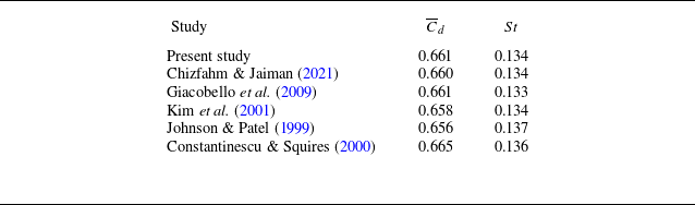
was first considered. The drag coefficient and Strouhal number were computed and compared with the results reported by Johnson & Patel (Reference Jiang, Pfister, Huang and Cao1999), Kim, Kim & Choi (Reference Jonathan, Clarence, Dirk, Steven and Kutz2001), Giacobello et al. (Reference Gharib2009), Chizfahm & Jaiman (Reference Cheng, Zhang, Wang, Lien and Dowell2021) and Constantinescu & Squires (Reference Chizfahm, Joshi and Jaiman2000) (see table 2). The present results are in close agreement with the reference data, indicating that the numerical method and mesh resolution are suitable for the simulations.
Comparison of computed time-averaged drag coefficient,
 $\overline {C}_d$
, and Strouhal number,
 $St$
, for steady sphere at
 $Re$
= 300 with other numerical studies.

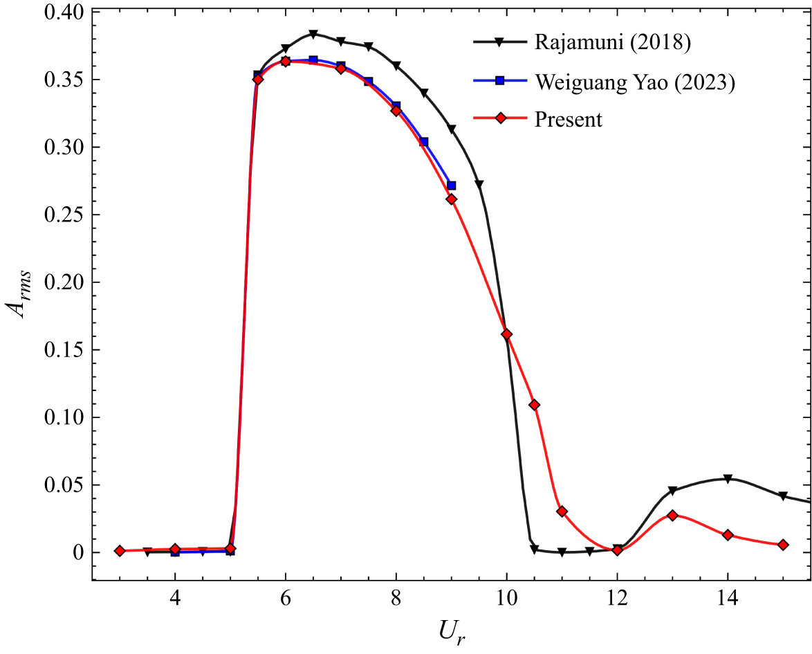
Further validation of the FSI model was carried out by simulating a 3-D sphere undergoing single-DOF transverse FIV in uniform flow. The simulations adopted the same parameters as Rajamuni et al. (Reference Rajamuni, Hourigan and Thompson2018a
) and Yao et al. (Reference Yao and Jaiman2023a
), with
 ${\textit{Re}} = 300$
,
 $m^{*} = 2.865$
and
 $\zeta = 0$
. The transverse amplitude
 $A_{\textit{rms}}$
was computed and compared with the reference data (see figure 3). The good agreement confirms the reliability of the FSI algorithm and the associated code used in the present simulations. While a direct validation for the prolate spheroid geometry would be ideal, benchmark data for this specific shape and Reynolds number are currently unavailable in the literature. Consequently, confidence in the present results is established through the rigorous validation of the solver against the canonical 3-D sphere case, combined with the strict grid independence study presented in table 1.
Comparison of the amplitude of transverse flow-induced vibration for an elastically mounted sphere with a single degree of freedom at
 $Re$
= 300 ,
 $m^{*} = 2.865$
and
 $\zeta = 0$
.

3. Results and discussion
In the study, we present the characterisation and analysis of the system’s dynamical behaviour, including vibration responses, wake dynamics, hysteresis and stability. To gain deeper insight into the underlying mechanisms, the dynamics are further examined using dynamic mode decomposition (DMD) and an ERA-based reduced-order model (ROM). The present simulations are conducted at a moderate Reynolds number of
 ${\textit{Re}} = 600$
, under which the system exhibits complex nonlinear fluid–structure interaction (FSI) characteristics. With a fixed aspect ratio of
 $\epsilon = 3$
, the spheroid’s slender geometry gives rise to vibration responses that differ markedly from those of a 3-D sphere and display more intricate patterns. The structural parameters are specified as a mass ratio of
 $m^{*} = 3$
and zero structural damping
 $(\zeta = 0)$
. The study focuses on the effects of reduced velocity (
 $0 \lt U_r \leqslant 25$
) on the FSI dynamics and examines the dependence of the system response on distinct initial conditions.
3.1. Vibration responses of the spheroid
Based on our simulations across a wide range of reduced velocities, the spheroid exhibits five distinct vibration modes as
 $U_r$
increases: the quasi-steady (QS), the periodic (PM), the large-amplitude chaotic (LAC), the quasi-periodic (QP) and the small-amplitude chaotic (SAC) modes. These classifications provide a framework for interpreting the system’s vibrational responses in the following discussion. Figure 4 presents the vibration response for a representative case from each vibration regime, including the amplitude time history, as well as the corresponding wavelet transform and FFT results. The wavelet transform captures instantaneous frequencies and is particularly effective for analysing FIV, while the FFT provides the global frequency content of the vibration signal. The combination of these methods offers a clear depiction of frequency evolution during vibration.
Amplitude time histories of a spheroid at various velocities, corresponding wavelet transform contour plots, and fast Fourier transform frequency spectra for oscillation and
 $z$
-direction lift frequencies: (a)
 $U_r=3$
; (b)
 $U_r=4$
; (c)
 $U_r=10$
; (d)
 $U_r=18.3$
; (e)
 $U_r=25$
.

Figure 4(
 $a$
) illustrates the case of
 $U_r = 3$
, corresponding to the QS mode. The vibration amplitude rises rapidly at first, then decays gradually and eventually oscillates slightly around zero. The wavelet contour reveals a progressive decrease in oscillation intensity over time, with the frequency remaining nearly constant. This behaviour is corroborated by the Fourier spectrum, which shows a single dominant frequency of 0.259 accompanied by multiple lower-frequency peaks. Notably, the dominant oscillation frequency remains equal to the
 $z$
-direction lift frequency, i.e.
 $f_{\textit{osc}} \approx f_{lz}$
.
For the case of
 $U_r = 4$
corresponding to the PM mode, shown in figure 4(
 $b$
), the vibration amplitude rises rapidly to a maximum value and then exhibits sinusoidal periodic oscillations. Both the wavelet and Fourier spectra indicate a single frequency of
 $f_{\textit{osc}} = 0.204$
, which corresponds to the
 $z$
-direction lift frequency in this regime.
For the case of
 $U_r = 10$
corresponding to the LAC mode, as shown in figure 4(
 $c$
), the vibration exhibits a disordered pattern. Compared with the
 $U_r = 4$
case, the vibration amplitude decreases and fluctuates irregularly over time. This irregularity gives rise to a wide range of frequency components, most of which are lower than the dominant frequency (
 $f_{{osc}} = 0.086$
), all clearly identified in both the wavelet and Fourier spectra. Moreover, despite the broad spectral characteristics of the vibration, the dominant oscillation frequency remains equal to the
 $z$
-direction lift frequency, consistent with the behaviour observed in the QS and PM regimes.
For the case of
 $U_r = 18.3$
corresponding to the QP mode, as shown in figure 4(
 $d$
), the vibration amplitude remains high and gradually stabilises at its maximum value over time, exhibiting a quasi-periodic pattern resembling a sinusoidal waveform. The wavelet contour shows that the oscillation frequency increases slowly at first and then stabilises at a dominant value of 0.056 once a steady state is reached. The Fourier spectrum reveals a dominant
 $z$
-direction lift frequency of 0.172, approximately three times the oscillation frequency, i.e.
 $f_{lz} \approx 3f_{\textit{osc}}$
.
When
 $U_{r}$
is increased to 25 corresponding to the SAC mode, as shown in figure 4(
 $e$
), the vibration amplitude initially rises to a high level, but then decays rapidly, exhibiting irregular patterns similar to those at
 $U_{r} = 10$
, though with much smaller amplitude. The Fourier spectrum analysis for the vibration identifies several frequency components, each of which is either lower than or approximately equal to the lift frequency in the
 $z$
-direction (0.141). In this mode, the dominant vibration frequency is
 $f_{\textit{osc}} = 0.012$
, a subharmonic of the natural frequency (
 $F = 1/U_r = 0.04$
), with
 $f_{\textit{osc}}/F = 3/10$
.
Phase portraits and Poincaré sections of the spheroid’s transverse displacement (
 $z$
) and its time derivative (
 $ \text{d}z/\text{d}t$
,
 $\text{d}^2z/\text{d}t^2$
) under varying flow conditions: (a)
 $U_r=3$
; (b)
 $U_r=4$
; (c)
 $U_r=10$
; (d)
 $U_r=18.3$
; (e)
 $U_r=25$
.

Figure 5 presents the spheroid’s displacement phase trajectories in phase space, together with their intersection points on the Poincaré section. A phase trajectory describes the evolution of a dynamical system in phase space, where displacement
 $z$
, velocity
 $\text{d}z/\text{d}t$
and acceleration
 $\text{d}^{2}z/\text{d}t^{2}$
serve as the coordinate axes. The Poincaré section facilitates the analysis of system periodicity or chaotic behaviour by recording trajectory intersections on a cross-sectional plane in phase space (Jiang et al. Reference Jauvtis and Williamson2025).
The phase trajectory characterises the system’s oscillatory behaviour, indicating periodic motion when it forms a simple closed curve, akin to a limit cycle. This is the case in the PM mode: as shown in figure 5(
 $b$
), the trajectory forms a closed circular loop with a single intersection on the Poincaré section, confirming periodic motion. This observation is consistent with the sinusoidal waveform of the vibration in figure 4(
 $b$
), as well as the single dominant frequency identified in the FFT and wavelet spectra. In the QP regime, however, the trajectory shown in figure 5(
 $d$
) does not form a perfectly closed loop, but reveals partial periodicity. Accordingly, the intersection points on the Poincaré section are relatively clustered, which is characteristic of quasi-periodic motion.
In contrast, multiple overlapping closed loops indicate complex, non-periodic dynamics that is close to chaotic behaviour. As shown in figures 5(a), 5(c) and 5(e), the trajectories deviate markedly from the periodic case in figure 5(
 $b$
), displaying interwoven curves and multiple non-overlapping loops. These features are consistent with the broadband or multi-frequency spectra observed in the FFT and wavelet analyses, confirming the presence of multiple frequency components and strong nonlinear interactions. It is also noteworthy that in the QS case shown in figure 5(
 $a$
), the intersection points on the Poincaré section remain relatively concentrated owing to the spheroid’s very small vibration amplitude, even though the oscillation exhibits multi-frequency characteristics.
Together, the phase-space trajectories, FFT spectra and wavelet transforms provide a coherent depiction of the system dynamics: simple closed loops with a single dominant frequency confirm periodic motion in the PM mode; quasi-periodicity arises in the QP mode, characterised by clustered Poincaré intersections and dual-frequency components; whereas interwoven trajectories, along with the broadband features revealed by the FFT and wavelet analyses, clearly signify chaotic behaviour with strong nonlinear interactions in the QS, LAC and SAC modes.
To provide a quantitative characterisation of the system’s complex dynamics and facilitate the classification of amplitude regimes, the fractal dimension (
 $d_c$
) is employed. This metric quantifies the geometric complexity of fractal-like objects by capturing their irregularity and self-similarity. In flow-induced vibration, where the amplitude time history often exhibits nonlinear and irregular patterns, the fractal dimension offers an effective means to quantify the degree of complexity in the system’s response. The fractal dimension
 $d_c$
is defined as
 \begin{equation} d_c = \lim _{s \to 0} \frac {\log (C_p(s))}{\log (s)}, \end{equation}
where
 $C_p(s)$
denotes a function associated with the Hausdorff measure and
 $s$
is the scale parameter. The expression for
 $C_p(s)$
is
 \begin{equation} C_p(s) = \lim _{R \to \infty } \frac {1}{N^2} \sum _{\substack {i,j=1 \\ i \neq j}}^N h\left (s - \left | \boldsymbol{X}_i - \boldsymbol{X}_j \right | \right ), \end{equation}
where
 $ \boldsymbol{X}_i$
and
 $ \boldsymbol{X}_j$
represent the positions of particles
 $ i$
and
 $ j$
in a system of
 $ N$
particles,
 $ | \boldsymbol{X}_i - \boldsymbol{X}_j |$
denotes their Euclidean distance, and
 $h(\boldsymbol{\cdot })$
is the Heaviside function. The summation covers all distinct pairs
 $ (i, j)$
, with the prefactor
 $ (1/N^{2})$
providing normalisation. The limit
 $ R \to \infty$
corresponds to the thermodynamic limit.
Response characteristics versus
 $U_r$
. (a) Root-mean-square (r.m.s.) of the amplitude,
 $A_{\textit{rms}}$
. (b) The dynamic parameter
 $d_c$
. The plot is divided into five distinct response regimes, indicated by different background colours: QS, PM, LAC, QP and SAC.

Figures 6(
 $a$
) and 6(
 $b$
) show the r.m.s. amplitude
 $A_{\textit{rms}}$
and the corresponding fractal dimension
 $d_c$
as functions of the reduced velocity
 $U_r$
, respectively. Following the definition of fractal dimension (Grassberger & Procaccia Reference Govardhan and Williamson1983),
 $d_c \approx 1$
corresponds to regular periodic motion, whereas
 $d_c \gt 1$
reflects increasing irregularity, with larger deviations from unity indicating stronger chaotic behaviour. Combining amplitude data, phase-space trajectories and
 $d_c$
variation, the vibration responses are classified into five regimes with their respective ranges of
 $U_r$
: the quasi-steady (QS,
 $0 \lt U_r \leqslant 3$
), periodic (PM,
 $3 \lt U_r \lt 10$
), large-amplitude chaotic (LAC,
 $10 \le U_r \lt 15$
), quasi-periodic (QP,
 $15 \le U_r \lt 21$
) and small-amplitude chaotic (SAC,
 $21 \lt U_r \leqslant 25$
) regimes.
In the QS regime (
 $0 \lt U_r \leqslant 3$
), the spheroid displays minimal vibration (figure 6
 $a$
), akin to the initial phase encountered in circular-cylinder FIV. Additionally, the fractal dimension
 $d_c$
is challenging to ascertain because of the exceedingly low amplitude. In the PM regime (
 $3 \lt U_r \lt 10$
), the vibration stabilises into a well-defined periodic pattern (figure 4
 $b$
), with
 $d_c$
remaining very close to unity (figure 6
 $b$
) and the vibration amplitude maintaining high values (figure 6
 $a$
), providing a clear quantitative basis for defining this regime.
Based on the variation of
 $d_c$
with
 $U_r$
, the ranges of the three remaining non-periodic regimes can be delineated. As
 $U_r$
increases beyond 10,
 $d_c$
deviates markedly from unity and stabilises around 1.5 for
 $10 \le U_r \lt 15$
(figure 6
 $b$
), indicating pronounced chaotic behaviour, consistent with the phase trajectories and FFT results. In this range, the system enters the LAC regime, exhibiting reduced amplitude compared with the PM regime and a distinctly aperiodic response. Between the LAC and SAC regimes, the QP regime occurs for
 $15 \le U_r \lt 21$
, where
 $d_c$
is above unity but lower than that in the LAC and SAC regimes (figure 6
 $b$
), reflecting quasi-periodic motion. The vibration amplitude in this region is considerably higher than in the LAC and SAC regimes, while the degree of chaos remains slight. Finally, for
 $21 \lt U_r \leqslant 25$
,
 $d_c$
exceeds 1.5, as shown in figure 6(
 $b$
), indicating stronger nonlinearity and high levels of chaotic behaviour; the system is classified within the SAC regime, characterised by very small amplitude yet highly irregular vibrations.
The amplitude curve shown in figure 6(
 $a$
) exhibits two distinct peaks, rising with
 $U_r$
, then falling, rising again and finally decreasing. Owing to the spheroid’s slender geometry, the response follows a complex pattern, reflecting the interplay of multiple characteristic frequencies. To elucidate amplitude variations, it is essential to examine the key frequencies in FSI: the structural natural frequency (
 $f_n=1/U_r$
), oscillation frequency (
 $f_{\textit{osc}}$
),
 $y$
-direction lift frequency (
 $f_{ly}$
) and
 $z$
-direction (i.e. vibration direction) lift frequency (
 $f_{lz}$
). The competition and interaction among these frequencies govern the amplitude response and provide crucial insights into flow-induced vibration.
Building on this concept, the present study examines the frequency characteristics across all regimes to deepen understanding of three-dimensional FIV dynamics. It should be noted that, owing to the specific geometry of the slender prolate spheroid, two primary vortex shedding modes emerge as a function of
 $U_r$
(a detailed analysis is presented in § 3.2). One mode involves shedding along the spanwise (
 $y$
) direction, while the other occurs in the transverse (
 $z$
) direction. This variation in shedding orientation renders a single lift component inadequate for characterising the vortex shedding frequency. Consequently, the frequencies associated with the lift forces in the
 $y$
and
 $z$
directions, namely
 $f_{ly}$
and
 $f_{lz}$
, are investigated separately. Furthermore, since the present study focuses exclusively on the spheroid’s vibration in the transverse (
 $z$
) direction,
 $f_{lz}$
emerges as the dominant factor governing the response and therefore warrants detailed examination.
Figure 7 shows the system’s typical frequency characteristics versus
 $U_r$
:
 $f_{ly}$
,
 $f_{lz}$
,
 $f_{\textit{osc}}$
and
 $f_n$
(figure 7
 $a$
); the frequency ratio
 $f_{lz}/f_n$
, with squares indicating the dominant frequency (figure 7
 $b$
); and the phase difference between structural vibration and
 $z$
-direction lift (figure 7
 $c$
). In the QS regime, vortices shed alternately from the spanwise sides (see figure 8) and the associated shedding frequency aligns with the lift frequency in the
 $y$
-direction. As illustrated in figure 7(
 $a$
), this frequency is close to the Strouhal number corresponding to vortex shedding of the stationary spheroid (
 $St = 0.4$
, see figure 11). Since the lift in the
 $y$
-direction is perpendicular to the vibration, it does not directly drive the structural response. In contrast, the lift in the
 $z$
-direction exhibits multiple frequency components, with dominant peaks deviating markedly from the structure’s natural frequency, while the structural amplitude remains negligible. This indicates a quasi-steady, multi-frequency, flow-induced forced response in the
 $z$
-direction, without any significant flow-structure synchronisation. The
 $z$
-direction lift nonetheless governs the vibration dynamics and simultaneously exerts a restoring effect. This finding underscores the significant influence of flow-induced modes in determining the spheroid’s vibration behaviour, which will be explored in detail in the stability analysis provided in § 3.5.
Dynamic response characteristics as a function of the reduced velocity
 $U_r$
. (a) Comparison of the transverse fluid force frequency
 $f_{lz}$
, the spanwise fluid force frequency
 $f_{ly}$
, and the structure’s oscillation frequency
 $f_{\textit{osc}}$
with the natural frequency of the structure,
 $f_n$
(
 $=1/U_r$
, dashed line), and the frequency corresponding to a fixed spheroid,
 $St = 0.4$
(dash-dotted line). (b) Power spectral density (PSD) contour of the frequency ratio
 $f_{lz}$
/
 $f_n$
, where the colour intensity represents the energy level. Five different synchronisation and desynchronisation mechanisms are identified: flow-dominated desynchronised (FDD), conventional lock-in (CLI), secondary-component lock-in (SCLI), superharmonic lock-in (SHLI) and dual-mode competition desynchronised (DMCD). (c) Phase difference
 $\phi$
between the
 $z$
-direction fluid force and the structural displacement.

In the PM regime, vortices shed alternately along the vibration direction (see figure 8), with
 $f_{lz}$
reflecting the dominant shedding frequency; this shedding orientation differs from that in other regimes. As illustrated in figure 7(
 $a$
),
 $f_{ly}$
and
 $f_{lz}$
are nearly equivalent, maintain synchronisation with the oscillation frequency (
 $f_{\textit{osc}}$
) and both converge towards the natural frequency (
 $f_n$
). The occurrence of frequency lock-in leads to the phenomenon of resonance. Unlike the case of a sphere, the frequency ratio stabilises around 0.9 rather than 1 (see figure 7
 $b$
), likely due to the spheroid’s slender geometry. This resonance results in a sharp increase in amplitude, with the oscillations exhibiting an almost sinusoidal pattern.
Within the LAC regime, the vortex shedding direction shifts from the vibration-aligned
 $z$
-axis, typical of the PM regime, to a spanwise (
 $y$
) orientation. As a result,
 $f_{ly}$
becomes the dominant shedding frequency, deviating from and exceeding both
 $f_{n}$
and
 $f_{lz}$
(see figure 7
 $a$
). This indicates that vortex shedding perpendicular to the vibration direction governs the near-wake dynamics, but has no direct influence on the spheroid’s vibration response. Unlike the conventional lock-in of the PM regime, where a dominant flow frequency locks to
 $f_n$
and yields periodic resonance, the LAC mode features a failure of the dominant
 $f_{ly}$
to synchronise with
 $f_n$
. Instead, a secondary component
 $f_{lz}$
locks to both
 $f_n$
and
 $f_{\textit{osc}}$
, while its weak multi-frequency subcomponents collectively disrupt periodicity, producing moderately large, chaotic oscillations (see figures 4
 $c$
and 7
 $b$
). We define this new mechanism as ‘secondary-component lock-in (SCLI) resonance’: a non-conventional lock-in phenomenon in which a non-dominant flow frequency component, rather than the dominant one, synchronises with the natural frequency of the structure. Moreover, under the SCLI, both the dominant frequency
 $f_{ly}$
and the locked frequency
 $f_{lz}$
deviate from the
 $St$
-law characteristic of the QS regime, as shown in figure 7(
 $a$
).
In the QP regime,
 $f_{ly}$
rises sharply to a nearly constant value close to the Strouhal frequency (
 $St = 0.4$
), corresponding to a spanwise vortex shedding mode similar to that observed for the stationary spheroid. Simultaneously, figures 7(
 $a$
) and 7(
 $b$
) reveal a rapid increase in
 $f_{lz}$
, maintaining
 $f_{lz}/f_{n} \approx 3$
in the QP regime, while the spheroid continues to oscillate at its natural frequency with large amplitude. This behaviour indicates the occurrence of a superharmonic resonance, in which the flow-induced frequency in the
 $z$
-direction locks onto three times the natural frequency of the structure. Unlike the conventional 1:1 lock-in observed in the PM regime, the structural response under this 3:1 superharmonic lock-in (SHLI) exhibits large-amplitude, low-frequency oscillations. Although the flow frequency represented by
 $f_{lz}$
does not match the fundamental natural frequency directly, its harmonic relationship is sufficient to excite the structure, resulting in quasi-periodic motion characterised by multiple frequency components. This demonstrates that high-order frequency synchronisation between the flow and the structure can significantly influence vibration dynamics, producing large-amplitude oscillations even when the fundamental lock-in mechanism is not active. Notably, the phase difference
 $\phi$
shifts from 0 in the QS, PM and LAC regimes to approach
 $\pi$
in the QP mode, indicating that the
 $z$
-direction lift force becomes nearly anti-phase with the spheroid oscillation. This highlights the distinction between the superharmonic lock-in (SHLI) phenomenon, and both the conventional lock-in (CLI) and the secondary-component lock-in (SCLI) resonance.
Finally, in the SAC regime, the lift frequencies
 $f_{ly}$
and
 $f_{lz}$
become nearly equal, and no longer lock onto the natural frequency
 $f_n$
, while the oscillation frequency
 $f_{\textit{osc}}$
also deviates from
 $f_n$
, confirming the absence of lock-in. Figure 4(
 $e$
) further shows a dominant vibration frequency of 0.012, accompanied by two secondary peaks located near
 $f_n$
( = 1/
 $U_r$
= 0.04) and
 $f_{lz}$
( = 0.141). These results collectively suggest that the response arises from the combined contributions of structural and flow modes; however, as
 $f_{lz}$
,
 $f_n$
and
 $f_{\textit{osc}}$
diverge and assume distinct values, resonance is lost, giving rise to low-amplitude, highly irregular vibrations. The mechanism underlying this desynchronised unstable mode can be described as a competing flow–structure instability, where both fluid and structural modes are unstable (see § 3.5), yet their frequencies deviate from the natural frequency. The resulting competition suppresses synchronisation and yields a complex, multi-frequency response. Notably, this mode contrasts with the QS desynchronised instability, in which the flow is unstable but the structure remains nearly stationary (see § 3.5), thereby revealing two distinct pathways of non-synchronised vibration dynamics.
In summary, three types of flow–structure synchronisation are identified in the spheroid’s vibration regimes: conventional lock-in (CLI, PM regime), secondary-component lock-in (SCLI, LAC regime) and superharmonic lock-in (SHLI, QP regime). CLI occurs when the dominant vortex shedding frequency matches the structural natural frequency, producing large-amplitude, nearly periodic oscillations. SCLI arises when a non-dominant flow frequency along the vibration direction locks onto the natural frequency, leading to moderately large, multi-frequency, chaotic vibrations. SHLI occurs when a flow-induced frequency locks onto an integer multiple of the natural frequency, exciting quasi-periodic motion. These mechanisms differ in which flow frequency locks to the structure (dominant versus secondary), the harmonic relationship (1:1 versus higher-order) and the resulting oscillation characteristics (periodic, chaotic or quasi-periodic). Here, it is noteworthy that the term ‘superharmonic lock-in’ refers to the synchronisation of a higher-harmonic lift-force frequency with the fundamental structural oscillation, rather than a superharmonic structural response in the classical sense. Beyond the lock-in regimes, no frequency synchronisation or resonance is observed in the QS and SAC modes. In the QS regime, structural vibrations remain weak and are primarily flow-dominated, whereas in the SAC regime, the interaction and competition between flow and structural frequencies lead to low-amplitude, low-frequency, and highly irregular vibrations.
3.2. Fluid field and wake dynamics
The spheroid exhibits distinct dynamic responses across different
 $U_r$
, driven by fluid–structure interaction. These motions, in turn, reshape the surrounding flow, producing characteristic vortex shedding and wake patterns. In this section, three representative shedding modes are identified, namely spanwise shedding (SS) in QS, LAC and SAC modes, transverse shedding (TS) in PM mode, and high-frequency spanwise shedding (HFSS) in QP mode.
Vorticity fields and 3-D vortex structures of the spheroid undergoing FIV: (a–d) spanwise shedding (SS) at
 $U_r=3$
; (e–h) transverse shedding (TS) at
 $U_r=4$
; (i–l) high-frequency spanwise shedding (HFSS) at
 $U_r=18.3$
. The first three columns display instantaneous
 $z$
-vorticity contours on the
 $y=0$
plane, the
 $z=Z$
plane and a downstream cross-section at
 $x=2$
; the last column gives the corresponding 3-D coherent vortex structures visualised by
 $Q$
-criterion isosurfaces.

Figure 8 illustrates the instantaneous wake vorticity fields and 3-D vortex structures for the SS, TS and HFSS patterns. In the SS pattern, which appears in the QS, LAC and SAC modes, the shear layers enveloping the spheroid shed alternately from the left and right sides along the
 $y$
-direction, forming staggered ‘U’-shaped (horseshoe) vortices in the wake, as shown in figure 8(
 $d$
). The downstream extension and subsequent breakdown of these shear layers are more clearly seen in the vorticity contours on the
 $z=Z$
plane (figure 8
 $b$
). This vortex structure differs from that in the TS pattern, corresponding to the PM mode, where the shear layers covering the spheroid detach from the ends of the major axis due to its large-amplitude oscillations, generating ‘
 $\varOmega$
’-shaped (hairpin) vortices in the wake, accompanied by contrail vortices that connect the spheroid surface or link adjacent hairpin vortices (see figure 8
 $h$
). These vortical structures correspond to the meandering wake observed on the
 $y=0$
plane (figure 8
 $e$
), while the flow remains symmetric on the
 $z=Z$
and
 $x=2$
cross-sectional planes (figures 8
f and 8
g). In the QP regime, the HFSS pattern, akin to the SS pattern, is typified by lateral shedding that generates horseshoe vortices. The distinguishing feature of this pattern is that, because of the sizeable oscillations of the spheroid in the
 $z$
-direction, numerous horseshoe vortices are released during a single upward movement. This leads to a shedding frequency that substantially exceeds the structural vibration frequency (refer to figure 4
 $d$
). Consequently, the vortex structures display significantly reduced spatial scales, as depicted in figure 8(
 $i{-}l$
). Notably, the wake manifests an oblique configuration (figure 8
 $i$
) and the associated shear layer is more diminutive than what is observed in the SS mode (figure 8
 $j$
).
To clearly illustrate the formation mechanisms of the two identified vortex structures – ‘U’-shaped (horseshoe) vortices and ‘
 $\varOmega$
’-shaped (hairpin) vortices – we next present representative cases of the SS and TS modes, highlighting the dynamics of shear-layer evolution, detachment and vortex formation around the spheroid at characteristic time instants.
Figure 9 chronologically illustrates the process of lateral vortex shedding in the SS mode, capturing the topological evolution of three-dimensional coherent structures in the spheroid wake over one complete cycle of horseshoe-vortex formation and shedding (
 $t_1$
–
 $t_4$
, corresponding to the first to fourth rows). Figure 9
 $(a)$
presents the top view of the vortex structures clipped in the
 $y=0$
plane, while the corresponding opaque visualisation is shown in figure 9
 $(b)$
. The third and last columns further provide complementary 3-D perspectives of the vortical structures from lateral and oblique viewpoints, respectively, together revealing the full three-dimensional topology of the wake evolution.
Instantaneous evolution of 3-D vortex structures for
 $U_r=3$
(SS mode) within one shedding cycle. Each row corresponds to a time instant, while the four columns present different views: clipped front view with vorticity contours on the
 $y=0$
plane, top view, full front view and oblique view. Vortices from the left and right sides of the bluff body are labelled JSL-L and JSL-R, where the numbers indicate shedding order; key flow features like the jellyfish-shaped shear layer, horseshoe vortex and vortex legs are also highlighted. The velocity direction of the ellipsoid is denoted by the purple arrow.

At the initial instant (
 $t_1$
), with the spheroid moving upward along the
 $z$
-axis, a jellyfish-shaped shear layer (JSL) wraps around the spheroid surface and extends downstream to form an asymmetric vortical structure in the near wake. This structure features a compact, nascent portion attached to the left side of the spheroid (denoted as JSL-L1) and an elongated, mature portion attached to the right side (denoted as JSL-R1), as shown in figure 9
 $(a{-}d)$
. Due to the inherent instability of the JSL during the unidirectional motion of the spheroid, both JSL-R1 and JSL-L1 continue to stretch downstream over time (see figure 9
 $(e{-}h)$
), until JSL-R1 undergoes the first breakup. Figure 9
 $(i{-}l)$
illustrates the state at
 $t_3$
, where JSL-R1 splits into two parts: one detaches to form a horseshoe vortex (HSV), while the remaining portion remains attached to the spheroid (JSL-R2). Subsequently, at
 $t_3$
and
 $t_4$
(see figure 9
 $m{-}p$
), JSL-L1 and JSL-R2 together form a new asymmetric jellyfish-shaped vortical structure, serving as the cradle for the formation of the next horseshoe vortex on the opposite side.
Instantaneous evolution of 3-D vortex structures for
 $U_r=4$
(TS mode) within one shedding cycle. Each row corresponds to a time instant, while the four columns present different views: clipped front view with vorticity contours on the
 $y=0$
plane, full front view, top view and oblique view. Vortices from the upper and lower sides of the bluff body are labelled JSL-U and JSL-D, where the numbers indicate shedding order; key flow features like the jellyfish-shaped shear layer, hairpin vortex and vortex legs are also highlighted. The velocity direction of the ellipsoid is denoted by the purple arrow.

Following the approach used for the horseshoe vortices (figure 9), figure 10 illustrates the dynamical evolution of hairpin vortices in the TS pattern. At
 $t_1$
, the spheroid undergoes a large-amplitude upward oscillation (indicated by the purple arrow in figure 10
 $a$
). In contrast to the SS pattern, the jellyfish-shaped shear layer (JSL) encircling the spheroid and stretching downstream exhibits mirror symmetry with respect to the
 $y=0$
plane (refer to figure 10
 $c$
). However, cross-sectional slices in the
 $x$
–
 $z$
plane at
 $y=0$
reveal an asymmetric configuration (figure 10
 $a$
), where the fully developed shear layer on the upper surface along the spheroid’s major axis (JSL-U1) extends farther downstream than the nascent shear layer on the lower surface (JSL-D1). As the spheroid reaches its maximum displacement and begins moving downward (figure 10
 $e$
–
 $h$
), the JSL undergoes partial detachment, forming a nascent hairpin vortex (HPV), while the remaining portion remains attached as JSL-U2. At this stage, the attached JSL-U2 and JSL-D1 stretch downstream to form a new asymmetric JSL structure (figure 10
 $i$
–
 $l$
), preparing for the formation of subsequent hairpins on the bottom side (figure 10
 $m$
–
 $p$
).
In the TS mode, the hairpin vortices detach from the JSL and form independently when the spheroid reaches its maximum or minimum displacement. This process is primarily governed by the frequency lock-in between the spheroid’s oscillation and the vortex shedding, rather than by the intrinsic instability of the shear layer as in the SS mode. Consequently, this promotes earlier instability and shorter streamwise scales compared with horseshoe vortices (HSVs). Notably, although resembling vortex rings, these hairpins are open structures connected to the spheroid’s leeward surface via two vortex tubes, referred to as vortex legs.
3.3. Dynamic mode decomposition of flow structures
Dynamic mode decomposition (DMD) is a widely used data-driven technique for extracting coherent spatiotemporal structures from complex flows (Peter Reference Peskin2010; Jonathan et al. Reference Johnson and Patel2014; Kutz et al. Reference Kim, Kim and Choi2016; Schmid Reference Sarpkaya2022). In this study, the open-source library pyDMD (Demo, Tezzele & Rozza Reference Constantinescu and Squires2018; Ichinaga et al. Reference Hua, Zhu and Lu2024) is employed to analyse the flow field associated with the FIV of a 3-D spheroid. To systematically capture the flow characteristics across different reduced velocities, several representative cases are selected, including the fixed configuration (corresponding to an effectively zero-amplitude scenario) and FIV cases at
 $U_r=4$
and
 $18.3$
.
In the present implementation, the DMD state vector
 $\boldsymbol{x}$
consists of the three-dimensional velocity field
 $(u, v, w)$
across the entire fluid domain, sampled at a constant interval of
 $\Delta t = 0.2$
. To capture the relevant temporal dynamics, the snapshot sequences cover at least two complete vibration cycles following the establishment of a statistically steady state (comprising 421 snapshots for the stationary case, 151 for
 $U_r=4$
and 586 for
 $U_r=18.3$
). The standard DMD algorithm is applied without mean subtraction; consequently, the mean flow is identified as the zero-frequency Mode 0. The truncation rank
 $r$
is determined based on a 99 % energy retention criterion, yielding
 $r=30$
,
 $40$
and
 $70$
for the stationary, periodic (
 $U_r = 4$
) and quasi-periodic (
 $U_r = 18.3$
) cases, respectively.
As a first step, the flow field around the stationary spheroid is analysed to identify the dominant modes in the 3-D domain. The analysis uses flow field data spanning two periods of stable oscillation, sampled at intervals of 0.2, yielding a total of 421 snapshots. DMD provides comprehensive modal information – including frequency, growth rate, amplitude and spatial structure – enabling a detailed characterisation of the flow. The resulting DMD modes are presented in figure 11.
DMD analysis results for the stationary spheroid. (a) Spectrum illustrating the distribution of the real and imaginary parts of the eigenvalues; (b) amplitudes of the DMD modes; (c) time histories of lift and drag forces along with their FFT spectra; (d) vorticity contours on the y-plane and z-plane, and 3-D flow structures corresponding to the first three modes.

Figure 11(
 $a$
) shows the growth rates and frequencies of the first eight DMD modes. All modal growth rates are zero, confirming the stability of the flow. Figure 11(
 $b$
) presents the modal amplitudes, indicating that the first four modes dominate:
 $f_{w0} = 0$
,
 $f_{w1} = 0.4$
,
 $f_{w2} = 2 f_{w1}$
and
 $f_{w3} = 0.113$
. Since
 $f_{w2}$
is a harmonic of
 $f_{w1}$
, only
 $f_{w0}$
,
 $f_{w1}$
and
 $f_{w3}$
correspond to distinct physical features.
In DMD, the first mode (
 $f_{w0}=0$
) corresponds to the mean flow and typically exhibits the largest amplitude, reflecting the dominant steady component of the flow field. All other modes appear as complex-conjugate pairs, representing oscillatory or unsteady structures associated with vortex shedding and flow instabilities. Figure 11(
 $c$
) shows the time histories of the force components and their FFT spectra:
 $F_x$
and
 $F_z$
share a dominant frequency (
 ${\approx} 0.113$
) corresponding to
 $f_{w3}$
, whereas the dominant frequency of
 $F_y$
(
 ${\approx} 0.4$
) aligns with
 $f_{w1}$
. The early emergence of the
 $F_y$
-associated mode (
 $M_{w1}$
) suggests that spanwise (
 $y$
) vortex shedding is the primary driver of the unsteady flow, a conclusion further supported by the corresponding modal flow structures. Figure 11(
 $d$
) illustrates the cross-sectional vorticity fields and 3-D structures of
 $M_{w0}$
,
 $M_{w1}$
and
 $M_{w3}$
. All exhibit symmetry only about
 $y=0$
, consistent with symmetric spanwise loading. The
 $M_{w0}$
mode shows four cylindrical vortex tubes extending downstream, representing the mean flow. The
 $M_{w1}$
mode characterises dominant spanwise vortex shedding, while
 $M_{w3}$
represents a coupled mode with streamwise-transverse vortex shedding.
Overall, both wake morphology and DMD analysis indicate that although coupled streamwise and transverse modes affect the near-wake dynamics, the spanwise shedding (SS) pattern dominates the stationary spheroid flow, which is also observed in the QS, LAC and SAC modes. To extend this analysis, DMD is applied to the flow fields under different vibration regimes to investigate how fluid–structure interaction modifies the dominant modes and wake structures. We focus on two representative cases:
 $U_r = 4$
, corresponding to the PM case in the conventional lock-in (CLI) branch, and
 $U_r = 18.3$
, corresponding to the QP mode in the superharmonic lock-in (SHLI) branch. These cases illustrate transverse shedding (TS) and high-frequency spanwise shedding (HFSS) patterns, respectively.
DMD analysis results for the spheroid at
 $U_r$
= 4. (a) Spectrum illustrating the distribution of the real and imaginary parts of the eigenvalues; (b) amplitudes of the DMD modes; (c) vorticity contours on the y-plane and z-plane, and 3-D flow structures corresponding to the first three modes.

Figure 12 presents the DMD results for the flow field around the FIV spheroid at
 $U_r = 4$
, corresponding to the PM case in the conventional lock-in (CLI) branch. The analysis is based on two fully developed vibration cycles, comprising a total of 151 snapshots. Owing to the strictly periodic nature of the oscillation, the results exhibit perfect symmetry. Figure 12(
 $a$
) shows the growth rates and frequencies of the first nine modes. All modes have zero growth rates, confirming their stability. Figure 12(
 $b$
) illustrates the modal amplitudes, where the first mode corresponds to the mean flow and contributes most significantly. The remaining modes represent dynamic flow structures, including
 $f_{w1} = 0.199$
and its harmonic
 $f_{w2} = 2f_{w1} = 0.398$
. As also evident in figure 4(
 $b$
),
 $f_{w1}$
coincides with both the
 $f_{\textit{osc}}$
and vortex-shedding frequencies
 $f_{lz}$
at
 $U_r = 4$
.
Figure 12(
 $c$
) shows the
 $y$
-plane and
 $z$
-plane vorticity contours together with the spatial structures of the three dominant modes. All modes exhibit symmetry with respect to both the
 $y=0$
and
 $z=0$
planes. The mean mode
 $M_{w0}$
features four columnar structures extending downstream from the mid- and rear-body regions of the spheroid, spreading laterally along the
 $z$
-axis. The
 $M_{w1}$
mode represents the dominant dynamic structure, with vortices shed primarily from the upper and lower surfaces of the spheroid and convected downstream parallel to the
 $y=0$
plane; also, a pair of vortex rows forms on either side of the
 $z=0$
plane, distinctly different from the
 $M_{w1}$
mode of the stationary spheroid. These structural features indicate the presence of a transverse shedding (TS) pattern. The
 $M_{w2}$
mode, corresponding to the second harmonic of
 $M_{w1}$
, exhibits finer-scale vortex structures. Additionally, it is evident that
 $M_{w1}$
and
 $M_{w2}$
are symmetric with respect to both the
 $y=0$
and
 $z=0$
planes. Notably, all dynamic modes appear at
 $f_{w1}$
and its harmonic, indicating that the flow field is dominated by a single frequency at this stage. This finding aligns with the frequency characteristics of the PM regime, where
 $f_{lz}$
and
 $f_{ly}$
are nearly equal and synchronised with the oscillation frequency, as observed in figure 4(
 $b$
), confirming the resonance mechanism in the PM regime, in which the vortex shedding along the oscillation direction dominates the unsteady flow.
Evolution of the dominant frequency at
 $U_r = 4$
during the onset of oscillation: (a) time history of vibration amplitude from rest to the steady state and (b) evolution of the dominant frequency across the three stages.

DMD is employed to extract the dominant frequencies and corresponding spatial structures from the evolving flow field. For
 $U_r = 4$
, the FIV development can be divided into three phases: early (phase 1), intermediate (phase 2) and steady (phase 3) (see figure 13
 $a$
). Throughout these phases, the dominant frequency gradually increases from 0.179 to 0.201, while the mode shapes transition from asymmetric, unstable structures to symmetric, stable wake patterns, as shown in figure 13(
 $b$
). By phase 3, all modal growth rates approach zero, indicating a fully developed oscillatory state, consistent with the DMD spectrum (figure 12
 $c$
). This evolution demonstrates how the wake progressively organises into the transverse shedding (TS) pattern characteristic of the PM regime, highlighting that the fully developed oscillatory state arises through continuous adjustment of modal structures rather than instantaneously.
DMD analysis results for the spheroid at
 $U_r$
= 18.3. (a) Spectrum illustrating the distribution of the real and imaginary parts of the eigenvalues; (b) amplitudes of the DMD modes; (c) vorticity contours on the y-plane and z-plane, and 3-D flow structures corresponding to the first three modes.

Figure 14 presents the DMD results for the spheroid FIV at
 $U_r = 18.3$
, corresponding to the QP mode in the superharmonic lock-in (SHLI) branch. In this analysis, 586 snapshots spanning two post-stabilisation oscillation periods were used. Due to the quasi-periodic nature of the vibration, the flow field exhibits a high degree of symmetry.
As shown in figure 14(
 $a$
), the growth rates of the first 11 modes are zero, confirming their stability and consistency with the steady vibration amplitude history in figure 4(
 $e$
). Figure 14(
 $b$
) illustrates the modal amplitudes and frequencies. The zeroth mode, with the largest amplitude and zero frequency, represents the mean-flow mode. The first mode has a frequency of 0.053, corresponding to the structural vibration frequency at this stage. Modes 2–4 correspond to the second to fourth harmonics of the structural mode. In particular, the third-order mode has a frequency of 0.157, approximately three times that of the first-order structural mode, corresponding to
 $f_{lz}$
, which reflects unsteadiness in the
 $z$
-direction flow. The fifth mode captures a high-frequency component consistent with
 $f_{ly}$
, reflecting the HFSS pattern in the QP mode.
Figure 14(
 $c$
) shows vorticity contours on the
 $y=0$
and
 $z=0$
planes, along with the 3-D vortex structures of the 0th, 1st, 3rd and 5th modes. The 0th mode exhibits symmetry with respect to both planes, reflecting the mean-flow structure. In the HFSS regime, the shear layers primarily detach alternately from the sides (along the
 $y$
-direction), forming the characteristic horseshoe-vortex wake captured by the 5th mode (
 $M_{w5}$
). This mode contains significant high-frequency components associated with the SHLI mechanism. Notably, the vortices are mainly observed in the downstream wake, away from the spheroid, collectively confirming the flow-dominated nature of the 5th mode. In contrast, modes 1–4 are associated with structural vibrations, with their coherent vortex structures concentrated near the spheroid and along streamwise-extending vortex tubes, reflecting the influence of structural motion on the surrounding flow.
3.4. Response branches and hysteresis
A characteristic feature of flow-induced vibration systems is the emergence of distinct vibration response branches and the associated hysteresis phenomenon (Williamson & Roshko Reference Williamson and Govardhan1988; Behara et al. Reference Bearman2011). In this study, the vibration response of the prolate spheroid is examined under two initial conditions: (i) a bidirectional sweep of reduced velocity (increasing- or decreasing-
 $U_r$
) and (ii) release from an initially stationary state, as detailed in § 3.1. These approaches consistently reveal multiple stable branches in certain
 $U_r$
ranges, where the coexistence of different oscillation states gives rise to hysteresis. To capture the hysteresis effect,
 $U_r$
was varied with a step size of
 $\Delta U_r = 0.3$
, where each simulation was initialised from the steady-state solution, in a statistical sense, of the preceding step. Additional tests using smaller
 $\Delta U_r$
produced indistinguishable hysteresis characteristics, confirming that
 $\Delta U_r = 0.3$
is sufficient to resolve the bistable regions while maintaining computational efficiency.
Response branches and hysteresis of the FSI system. The r.m.s. amplitude (
 $A_{\textit{rms}}$
) as a function of
 $U_r$
is shown for three conditions: initially stationary (green diamonds), increasing-
 $U_r$
(blue squares) and decreasing-
 $U_r$
(pink inverted triangles). Arrows indicate the direction of the velocity sweep. The different paths for increasing and decreasing
 $U_r$
form clear hysteresis loops, highlighting the path-dependent nature of the system. The schematic bar chart at the bottom summarises the observed response regimes (QS, PM, LAC, QP, SAC) during forward and backward sweeps, explicitly marking the three bistable regions. Circled numbers correspond to the five dynamic branches: FDD, CLI, SCLI, SHLI and DMCD.

Bistable phenomenon of the spheroid at
 $U_r$
= 13.3 within the hysteresis-2 regime. (a) Time histories of vibration amplitude and lift force, together with the corresponding FFT spectra, on the increasing branch. (b) Time histories of vibration amplitude and lift force, together with the corresponding FFT spectra, on the decreasing branch.

As shown in figure 15, the vibration response of the spheroid can be broadly classified into two categories: desynchronised branches (DB) and synchronised branches (SB). The synchronised branches encompass three regimes: the conventional lock-in (CLI) branch, corresponding to the PM mode, characterised by classical frequency lock-in; the secondary-component lock-in (SCLI) branch, corresponding to the LAC mode; and the superharmonic lock-in (SHLI) branch, corresponding to the QP mode. In contrast, the desynchronised branches consist of two distinct regimes: the flow-dominated desynchronised (FDD) branch, corresponding to the QS mode, where the flow instability dominates while the structural response remains nearly suppressed; and the dual-mode competition desynchronised (DMCD) branch, corresponding to the SAC mode, where both fluid and structural instabilities coexist, but compete without synchronisation, leading to a complex, multi-frequency response. The overlapping regions of these branches highlight the sensitivity of spheroidal VIV to initial conditions and its inherently path-dependent nature, providing new insights into how different synchronisation modes compete and transition in spheroidal geometries.
The lower panel of figure 15 illustrates three distinct hysteresis regions. The first hysteresis region occurs in the overlap of branch 1 (FDD) and branch 2 (CLI) over the range
 $3.5 \lt U_r \lt 4$
, where the system may reside in either the QS or PM mode depending on the initial conditions. The second hysteresis region appears in the overlapping range of branch 2 (CLI) and branch 3 (SCLI) over
 $9.3 \lt U_r \lt 15$
. Figure 16 demonstrates the bistability at
 $U_r = 13.3$
: when the initial condition corresponds to increasing-
 $U_r$
, the system exhibits the CLI branch, whereas for stationary or decreasing-
 $U_r$
, the system adopts the SCLI branch. The third hysteresis region arises in the overlap of branch 4 (SHLI) and branch 5 (DMCD), spanning
 $15 \lt U_r \lt 24$
, where the system may occupy either the QP or SAC mode, as shown in figure 15. Moreover, the third hysteresis region is substantially wider than the first, which can be attributed to stronger flow–structure coupling and the participation of multiple frequencies. Collectively, these factors increase the system’s sensitivity to initial conditions and extend the range of bistable behaviour. In summary, the prolate spheroid exhibits five vibration branches whose overlapping ranges give rise to multi-stability and pronounced hysteresis. Notably, the path-dependent transitions among PM, LAC and QP reflect the interplay of different lock-in mechanisms, providing a coherent framework for understanding how synchronisation modes emerge, coexist and switch under varying flow conditions.
3.5. Linear stability analysis using ERA-based ROM
After identifying the dominant flow modes using DMD, this section introduces a reduced-order model (ROM) based on the eigensystem realisation algorithm (ERA) to analyse system stability and the evolution of FSI dynamics. The ERA-based ROM constructs a low-dimensional state-space model by extracting dominant modes from time-series data, substantially reducing computational cost while retaining key dynamical features. Unlike DMD, which primarily identifies flow modes, the ERA-based ROM captures the coupling between flow and structural modes, providing insight into the mechanisms governing modal evolution in FSI systems (Yao & Jaiman Reference Williamson and Roshko2017; Li et al. Reference Lee, Hourigan and Thompson2019; Cheng et al. Reference Cheng, Lien, Dowell, Yee, Wang and Zhang2024).
Root locus plot for FIV of a 2-D square cylinder at
 $Re$
= 150 and
 $m^*$
= 50.

To assess the accuracy of the proposed algorithm, the results are first compared with published data (Li et al. Reference Lee, Hourigan and Thompson2019; Cheng et al. Reference Cheng, Lien, Dowell, Yee, Wang and Zhang2024) for a 2-D square cylinder at
 ${\textit{Re}} = 150$
and
 $m^* = 50$
, as shown in figure 17. Because the ERA-based ROM is inherently data-driven, it is highly sensitive to the input data, with each eigenvalue directly dependent on the underlying CFD results. Consequently, differences in CFD outcomes, which arise from variations in mesh resolution, numerical schemes or solvers, inevitably lead to discrepancies in the eigenvalue decomposition. Nevertheless, the ERA-based ROM primarily emphasises the sign of the eigenvalues, which governs stability. As illustrated in figure 17, the overall trends are consistent and the transition points where eigenvalues change from positive to negative largely coincide, thereby confirming the reliability of the reduced-order model developed in this study.
The initial step in the ERA methodology entails deriving a base flow. Given the intricate nature of the three-dimensional flow field, merely enlarging the time step is inadequate for obtaining a stable solution. Consequently, alternative strategies must be employed. In this research, the steady flow is achieved by using the selective frequency damping (SFD) approach as proposed by Åkervik et al. (Reference Ye, Wei, Huang and Lu2006). To accelerate convergence towards the steady base flow while ensuring numerical stability, an adaptive multi-stage control strategy was employed rather than relying on fixed parameters. The procedure consisted of four phases: it initiated with a strong damping regime (
 $\chi =150, \varDelta =0.00125$
) to effectively suppress initial transients, followed by intermediate adjustments where
 $\chi$
was progressively reduced to 50 and 25 while
 $\varDelta$
was increased to 0.0125 and 0.1, respectively. Finally, a fine-tuning phase with
 $\chi =15$
and
 $\varDelta =0.2$
was applied to facilitate the ultimate relaxation to the steady state. By carefully adjusting the filter coefficient and the cutoff frequency, a base flow conducive to further ERA analysis is produced. Figure 18 illustrates the base flow obtained via SFD, showing contours of the
 $x$
-velocity on the
 $y=0$
and
 $z=0$
planes, along with a 3-D view. The resulting flow field is observed to be uniform and steady, providing a reliable initial condition for the ERA impulse response analysis.
Base flow of a stationary spheroid system at
 $Re$
= 600. (a)
 $x$
-velocity contour for the plane
 $y$
= 0; (b)
 $x$
-velocity contour for the plane
 $z$
= 0; (c) 3-D view of the velocity isosurface.

(a) First 50 singular values in the Hankel matrix for flow passing a spheroid at
 $Re$
= 600; (b) impulse response
 $C_{lz}$
provided by full-order model (FOM, i.e. CFD method) and corresponding values predicted by the ROM method.

After obtaining an accurate base flow, the second step in the ERA analysis involves acquiring the impulse response of the lift force. In this study, a pulse disturbance with an amplitude of
 $0.01D$
is applied in the
 $z$
-direction of the spheroid, and the subsequent lift variation is recorded. Once sufficient data are collected, system identification is performed to extract the eigenvalues. For the construction of the Hankel matrix, a size of
 $1000 \times 1000$
is employed. As illustrated in figure 19(
 $a$
), the eigenvalue spectrum shows that the first 50 modes exhibit rapid variation, while modes beyond the 50th order tend to stabilise, suggesting that retaining the first 50 modes is sufficient to capture the essential dynamics. With the Hankel matrix structure and truncation order determined, the ROM parameters are then computed based on the governing equations (2.36). Figure 19(
 $b$
) presents a comparison between the ROM results and those from the full-order CFD model. The close agreement confirms the appropriateness of the selected Hankel matrix size and truncation order, as well as the accuracy of the derived ROM parameters.
Linear stability analysis using ERA-based ROM: (a) root loci of structural and flow modes for the fluid–structure interaction reduced-order model of the spheroid; (b) variation of the real parts of the structural modal eigenvalues with
 $U_r$
; (c) variation of the imaginary parts of the structural modal eigenvalues with
 $U_r$
.

By coupling the reduced-order flow field model with the structural vibration equation, a reduced-order FSI model is obtained, i.e. (2.40). Singular value decomposition (SVD) of the eigenvalue matrix of the coupled system yields the eigenvalue distribution, which forms the basis for stability analysis. The structural mode (SM) corresponds to eigenvalues exhibiting pronounced variations near the natural frequency, whereas the wake modes (WM) are identified as the most unstable points in the eigenvalue spectrum. Modal identification reveals the presence of two distinct modes, namely SM and WM, as illustrated in figure 20(
 $a$
). The SM crosses the zero axis three times, reflecting the complexity of its evolution.
In the ERA-based ROM analysis, the evolution of SM with increasing
 $U_r$
is clearly delineated by its growth rate. Positive SM growth rates indicate modal instability, typically associated with large-amplitude vibrations, whereas negative or near-zero growth rates correspond to stable or neutrally stable modes. The SM exhibits alternating stability regimes: stable for
 $U_r \le 7.1$
, unstable for
 $7.2 \le U_r \le 11.8$
, weakly stable for
 $11.9 \le U_r \le 14.8$
and unstable again for
 $U_r \gt 14.8$
. In contrast, WM remains unstable throughout the examined range, reflecting persistent flow-driven unsteadiness. The SM frequency consistently fluctuates near the natural frequency, while the WM frequency captures the main flow-induced unsteadiness, consistent with observations in stationary cases.
The interplay between the SM and WM explains the characteristics of the major vibration stages. In the QS stage, SM is stable while WM dominates, resulting in low-amplitude structural responses driven primarily by flow unsteadiness. During the PM stage, both SM and WM are unstable, producing large-amplitude, traditional lock-in behaviour. In the LAC stage, the weakly stable SM interacts with the unstable WM, giving rise to second-component lock-in features. For the QP and SAC stages, both SM and WM are unstable; however, the ROM cannot fully distinguish between these two regimes due to its linear reduced-order formulation and the multi-frequency nature of the motion. As discussed previously, the QP mode is dominated by the superharmonic lock-in mechanism, whereas in the SAC regime, the flow and structural frequencies compete without achieving frequency synchronisation. Consequently, although both SM and WM are unstable in the QP and SAC regimes, the differing modal coupling mechanisms lead to substantially different amplitude responses.
Notably, although the ROM successfully predicts the sequence of stable and unstable regimes across
 $U_r$
, the predicted instability boundaries, where the SM growth rate crosses zero, exhibit quantitative deviations from the full-order CFD results. Similar discrepancies were reported by Cheng et al. (Reference Cheng, Lien, Dowell, Yee, Wang and Zhang2024) in an ERA-based study of a 3-D cube, where the deviations were attributed to the inherent complexity of three-dimensional flow fields. These observations suggest that while the linearised reduced-order framework captures the essential physics, its quantitative precision is constrained by several fundamental factors.
First and foremost, the ERA-based ROM is inherently a linearised formulation constructed around a specific reference state. Consequently, it assumes a proportional coupling where fluid forces are treated as linear convolutions of structural motion. This framework cannot fully account for the amplitude- and history-dependent variations in effective added mass and damping that become prominent in high-amplitude regimes (Dowell & Hall Reference Demo, Tezzele and Rozza2001; Williamson & Govardhan Reference Sun, Peng, Yang, Xiong, Wang and Wang2004). Second, the modal truncation inherent in the ROM limits its capacity to represent higher-order Reynolds stresses and the nonlinear energy cascade between large-scale coherent structures and fine-scale fluctuations. Such multi-scale interactions are critical for energy saturation and can shift instability thresholds, yet they are only indirectly or partially captured in reduced systems (Noack et al. Reference Naudascher and Rockwell2003; Balajewicz & Dowell Reference Ye, Wei, Huang and Lu2012). Third, the current single-input–single-output (SISO) ROM framework, which focuses on
 $z$
-direction responses, represents a spatial simplification of the three-dimensional flow field. This approach may not fully account for the spanwise flow variations and vortex tilting across the spheroid. Such three-dimensional effects can influence the effective fluid forcing and may contribute to the observed shifts in stability thresholds (Jauvtis & Williamson Reference Ichinaga, Andreuzzi, Demo, Tezzele, Lapo, Rozza, Brunton and Kutz2004).
Crucially, this ERA-based identification tool is designed as a diagnostic instrument to detect the onset of instability. Its primary value lies in its ability to decouple the complex FSI system into distinct SM and WM contributions, thereby elucidating the competition mechanisms that drive the initial destabilisation. While the ROM effectively identifies the tendency for infinitesimal disturbances to grow, it does not account for the subsequent nonlinear intervention or the eventual saturated amplitude, which remain the domain of full-order nonlinear CFD.
4. Conclusions
In this study, the FIV of a slender prolate spheroid with
 $\epsilon = 3$
,
 $m^* = 3$
and
 $\zeta = 0$
, elastically mounted in a uniform flow at
 ${\textit{Re}} = 600$
, has been investigated using the lattice Boltzmann–immersed boundary (LBM-IB) method, supplemented by linear stability analysis to elucidate the underlying fluid-elastic instability mechanisms. The main conclusions are as follows.
Five vibration states emerge as
 $U_r$
increases, namely the quasi-steady (QS), periodic (PM), large-amplitude chaotic (LAC), quasi-periodic (QP) and small-amplitude chaotic (SAC) modes. These modes naturally divide into two response categories: synchronised branches (SB) and desynchronised branches (DB). Within SB, three lock-in mechanisms are identified. Conventional lock-in (CLI), associated with the PM mode, arises when the dominant vortex-shedding frequency locks to the structural natural frequency, producing large-amplitude, periodic oscillations. Secondary-component lock-in (SCLI), corresponding to the LAC mode, occurs when a secondary flow frequency along the vibration direction synchronises with the natural frequency, resulting in multi-frequency chaotic vibrations of moderately large amplitude. Superharmonic lock-in (SHLI), associated with the QP mode, emerges when the frequency induced by the flow becomes synchronised to an integer multiple (e.g. three times) of the natural frequency, thereby producing quasi-periodic vibration with large amplitude.
In contrast, the DB contains two distinct behaviours. The flow-dominated desynchronised (FDD) branch, corresponding to the QS mode, is characterised by unstable flow modes coexisting with a nearly stationary structure, yielding weak, flow-driven oscillations. The dual-mode competition desynchronised (DMCD) branch, associated with the SAC mode, arises from simultaneous but unsynchronised flow and structural instabilities, yielding a complex low-amplitude multi-frequency response.
Wake dynamics, strongly coupled with structural responses, exhibit three shedding patterns: spanwise shedding (SS) in QS, LAC and SAC modes, forming alternating U-shaped (‘horseshoe’) vortices; transverse shedding (TS) in PM mode, producing
 $\varOmega$
-shaped (‘hairpin’) vortices along the vibration direction; and high-frequency spanwise shedding (HFSS) in QP mode, arises from the decoupling of high-frequency horseshoe-vortex shedding from the primary oscillation.
The coexistence of multiple vibration branches across overlapping reduced-velocity ranges gives rise to pronounced hysteresis and multi-stability under three types of initial conditions (stationary, increasing-
 $U_r$
and decreasing-
 $U_r$
). Three distinct hysteresis zones are identified:
 $3.5\lt U_r\lt 4$
(FDD-CLI overlap),
 $9.3\lt U_r\lt 15$
(CLI-SCLI overlap) and
 $15\lt U_r\lt 24$
(SHLI-DMCD overlap). The mode transitions are strongly path-dependent, reflecting the sensitivity of spheroidal responses to initial conditions and the multiplicity of possible pathways.
Furthermore, DMD and the ERA-based ROM offer insights into the FSI instability. DMD identifies the flow modes and their spatial structures, whereas the ERA-based ROM reveals that the vibration dynamics is governed by a persistently unstable wake mode (WM) and a structural mode (SM) whose stability alternates with
 $U_r$
. The interplay between SM and WM governs the five vibration stages: in QS, a stable SM coexists with an unstable WM, yielding low-amplitude, flow-driven responses (FDD); in PM, simultaneous SM and WM instability produces large-amplitude, classical lock-in (CLI); in LAC, a weakly stable SM interacts with an unstable WM, giving rise to SCLI. While for QP and SAC, both SM and WM are unstable; in QP, superharmonic lock-in (SHLI) dominates, whereas in SAC, competing WM and SM prevent synchronisation, corresponding to the DMCD branch. Despite its linear, reduced-order form, the ROM captures key trends in modal growth and frequency evolution, underscoring the central role of fluid-elastic instability in governing the sequence, coexistence and transitions of vibration states.
Compared with a geometrically isotropic body such as a sphere, anisotropic geometries exemplified by the slender ellipsoid fundamentally reshape wake dynamics and FIV responses. For a sphere, the perfectly symmetric geometry allows the vortex shedding plane to drift relative to the vibration plane, particularly in the desynchronised regime at high reduced velocities (Rajamuni et al. Reference Rajamuni, Hourigan and Thompson2018a
). In contrast, the ellipsoid’s geometry anchors the shedding plane along its minor or major axis, maintaining a stable orientation relative to the vibration plane. This stabilisation strengthens the coherence of energy transfer from the flow to the structure, resulting in substantially larger vibration amplitudes in the high-
 $U_r$
branch (e.g. SHLI branch). These findings highlight how geometric modifications can fundamentally alter wake dynamics and vibration response, offering new perspectives for the control and use of flow-induced vibrations in engineering and bio-inspired applications.
While the present study offers a robust framework for understanding fluid-elastic instabilities, certain limitations warrant mention to clarify the scope of these findings. First, this investigation focused on a fixed geometry with an aspect ratio of
 $\epsilon =3$
. This choice facilitated a high-resolution sweep of the reduced velocity space, enabling the characterisation of five distinct vibration modes. Although the physical mechanisms identified at
 $\epsilon =3$
are considered representative of prolate spheroids in the intermediate aspect ratio regime, the specific modal boundaries are inherently sensitive to geometric changes, and further variations in
 $\epsilon$
may induce mode boundary shifts or even manifest distinct dynamic characteristics not observed in the present case. Second, the current model is restricted to 1-DOF transverse vibration. In realistic scenarios, the integration of rotational degrees of freedom may introduce complex trajectory tilting or the emergence of additional lock-in modes. Finally, the simulations were conducted at a fixed moderate Reynolds number (
 $Re=600$
). At significantly higher
 $Re$
, the onset of fully developed turbulence could modify the system’s damping properties and potentially narrow the synchronisation bandwidth. Future investigations addressing these geometric variations, multi-DOF coupling and high-Reynolds-number effects will be essential to further elucidating the physics of fluid-elastic instabilities in geometrically anisotropic bodies.
Funding
This research was supported in part by the National Natural Science Foundation of China (nos 12325201, 12372241, U22A20206) and the Natural Science Foundation of Hubei Province of China (no. 2022CFB131).
Declaration of interests
The authors report no conflict of interest.