“To arrive at some understanding of what is going on is hard enough,” said Abraham Kaplan, “without having also to meet the demand that we anticipate what will happen next” (1964, 351). Political scientists have been taught to describe and to explain phenomena rather than to predict them. Kaplan, for one, appeared to think that this was enough. But within the rich soil of explanation, Kaplan admitted (346), lay the seed of prediction. Indeed, Carl G. Hempel and Paul Oppenheim (1948, 138), whom Kaplan took to task for saying so, flatly stated that “an explanation is not fully adequate” unless it also served as the basis for prediction (quoted in Kaplan, 346).
We admit that many challenges present themselves when we attempt to predict complicated social phenomena. But we argue that there is a danger in limiting our research to description and explanation. That danger is that repeated analysis of the same datasets will track patterns again and again that do not exist in the reality outside our samples. One guard against this is to take theories about politics and employ them to predict events that have not yet happened. In this spirit, this paper utilizes well-known insights about congressional elections to predict the 2006 elections in the U.S House of Representatives.
Methods of predicting congressional election outcomes have fallen into two categories. In the first, experts used district- or state-level information to try to call elections. Sometimes these predictions were aided by district-level polls (of varying quality). CQ Politics has made such predictions for all House and Senate elections. The second method has used a more aggregate approach, examining past elections in order to compare the number of seats that change party hands with various measures of a national partisan tide. A national partisan tide was represented by such factors as the health of the economy, presidential approval, the quality of candidates running for each party, or voting intentions (Jacobson 2004; Abramowitz 2002). Using estimates of the magnitudes of these relationships, and taking the current values of the independent variables, predictions of future elections were then made (Abramowitz and Segal 1986; Abramowitz 2002, 2006). Each method has its strengths and weaknesses, but combining the two methods takes advantage of the strengths of both. The combined approach was taken in this paper.
The strength of the district-level approach was that it recognized the importance of district-level factors in influencing election outcomes. The weakness was that the district-level approach might not accurately assess the size of a national partisan tide. The strength of the aggregate approach was that it was better at assessing such a tide. Its weakness was that it did not assess how such a national partisan tide might interact with district-level factors. For example, if there were a large national partisan tide, its impact on how many seats change hands nationally would have been contingent on how many “swing districts”—districts won by only a few percentage points—existed. Similarly, the impact of the national tide on the electoral chances of “quality” challengers—a variable which has often been measured as challengers who have held elective office in the past (Jacobson 2004)—running in any particular House district for either party has been contingent on the history of House elections in the districts themselves. Attractive candidates running in historically very competitive districts have been more likely to win election. Attractive candidates running in only marginally competitive districts have been less likely to win election. Combining both approaches by using a panel model, that is, a model that combines many different time series into one pooled dataset, overcomes both of these problems. National and district conditions should be examined in detail, as well as how those conditions influence election outcomes in combination. The rest of this article explains this modeling strategy and its predictions for the 2006 midterm House elections.
Methodology
The general strategy utilized in this paper was to assess relationships between independent variables and election outcomes in past elections. Then, the values of these independent variables in 2006 were used to predict House election results in November, 2006. The dependent variable of this analysis was the percent of the two-party vote that went to Democrats in contested U.S. House of Representatives elections between 1974 and 2004. As we said earlier, a pooled design similar to the design others have used for House (McGhee 2004) and Senate (Highton 2000) elections was used here. Cases from the 1988 and the 1992 elections were excluded from the analysis for reasons explained below. Three general types of factors were used in the model to predict future election outcomes: district partisan composition, candidate attributes, and national partisan tides. All data used in this model, except for the national partisan tide variables, were from data generously provided by Gary Jacobson. (Variable names are set off by parentheses below.)
The partisan composition of districts was measured in two ways. The first was the two-party vote for Democrats from the most recent regularly scheduled House election in the district (“Past House Vote”). When no Democratic (Republican) candidate contested the last election, a “0” (“100”) was entered for this variable. An additional variable labeled “Last Election Uncontested” was included to relax the assumption that an election with no Democratic candidate was equivalent to a “0” for “Past House Vote” and “100” in the case ofno Republican candidate. It was coded “−1” when the last election was not contested by a Democrat, “1” when the election was not contested by a Republican, and “0” if otherwise. The variable was expected to have been negative in sign.
The second measure of the partisan composition of districts was the result from the most recent presidential election in the district, from which the percent of the Democratic two-party vote in the nation as a whole was subtracted (“Past Presidential Vote”). This was done so that national partisan tides favoring a certain party in a presidential election were subtracted out of presidential vote returns. (See Benjamin Highton [2000] for a full explanation.) The inclusion of this variable made it necessary to exclude the results of the 1992 presidential election from the analysis because presidential returns from 1988 were not available for 1992 districts. Only one past election was utilized because using the results of two past elections would have caused the loss of many cases due to redistricting.
Various attributes of House candidates were included in the model. Whether a candidate was an incumbent was measured (“Incumbent”). Whether a candidate had held a past elective office was measured by the two following variables: “Quality Candidate, Closed” measured such candidates when they faced an incumbent; “Quality Candidate, Open” measured such candidates contesting open seats in which two non-incumbents faced each other. Whether candidates had held seats previously in the House of Representatives was also considered. This variable also took into account whether these non-sitting House veterans were running against the present incumbent (“Past House Member, Closed,” and “Past House Member, Open”). These variables were coded “1” when only the Democratic candidate had these attributes, “−1” when only the Republican candidate had them, and “0” in all other instances. The ability of these attributes to obtain greater votes for a party has been well documented elsewhere (Jacobson 2004).
Four aspects of national partisan tides were measured. The first was the percent of respondents who expressed an intention to vote for a Democratic House candidate in the upcoming election. This expression of voting intention was recorded by the Gallup poll conducted closest to March 10 of even-numbered years (“Democratic Vote Intention”).1
These data are from www.gallup.com and were accessed in late March of 2006.
James Campbell (2003) argued that the rise of uncompetitive seats in the U.S. House has insulated its incumbents from partisan tides. According to Campbell, this insulation explained the small number of changes in House seats in recent elections. But it could be argued, looking at the Democratic vote intention in March 2006, that that insulation may crumble in November 2006. The Gallup March voting intention measure indicated that Democratic vote intention had been flat for every House election year between 1994 and the present. This is important because, in the aggregate, Democratic vote intention has been strongly correlated with the percent of seats that Democrats obtain in November (Pearson's r = .79). This year, though, there has been an abrupt rise in Democratic voting intention, according to Gallup. By this year's measure, this simple bivariate model predicted that the Democrats would obtain 57.6% of House seats in 2006.
This prediction is surely an overestimate. Such a change would constitute a 48-seat gain for the Democrats, and would raise the number of Democratic seats to 250. This change would give them a 65-seat bulge (250 to 185) over the Republicans. A reversal of that size would return the Democrats to the majority it last enjoyed over the opposition in the 103rd Congress (1993–1995) when former President William J. Clinton was in the White House and 258 Democrats controlled the House of Representatives. We think that our more elaborate model has more accurately assessed how this national tide will play itself out among the uncompetitive districts that have recently come into existence. We also argue that this research has marked out a more realistic assessment of Democratic chances of obtaining a House majority in November 2006.
The second national partisan tide factor we examined here was presidential approval (“Presidential Approval”)2
These data are from www.gallup.com and were accessed in late March of 2006.
The third national partisan tide variable was the relative advantage to each party brought by the performance of the economy. The strength of the economy was measured as the percent change that occurred in per capita real disposable income between the February of the year before the election year, and the February of the election year (“Change in Real Disposable Income”).3
These data come from the Bureau of Economic Analysis web site, in the Department of Commerce. Table 2.6 at www.bea.gov/bea/dn/nipaweb/selecttable.asp?selected=n, and were accessed April 9, 2006.
The fourth national partisan tide variable captured the tendency of the party of the president to lose votes in a midterm election (“Midterm Penalty”) (Jacobson 2004). This variable was coded “−1” for midterm elections in which a Democrat was in the White House, “1” for midterm elections in which a Republican was in the White House, and a “0” for presidential election years.
Findings
The variables in the model behaved much as expected.4
The Durbin's m test for autocorrelation indicates that there is first order autocorrelation (Gujarati 1995, 425–6), although it is extremely small in magnitude. In this test, when the residuals are regressed on all the independent variables and the lagged residuals, the resulting R-squared is a mere .022. With a dataset of this size (5,899 cases), it is very hard to fail to find autocorrelation because “n” appears in the formula. Also, the presence of autocorrelation does not influence the point estimates of the predictions (Gujarati 1995).
Determinants of Democratic Share of the Two-Party Vote in House Elections, 1974–2004

The four national partisan tide variables behaved as expected, and all were statistically significant. Every 1% more of “Democratic Vote Intention” was associated with .03% more votes for Democrats. The cumulative impact of a change in this variable across districts can be substantial. Every 1% more approval (disapproval) for a Democratic (Republican) president was associated with .10% more votes for Democratic candidates. Every 1% increase (decrease) in real disposable income under a Democratic (Republican) president was associated with .14% more votes for Democratic candidates. Beyond the variation captured by these measures, members of the president's party running in midterm House elections have been at a disadvantage. All else being equal, candidates of the president's party lose 3.6% of the vote in midterm years.
We also investigated a model that included interactions between a dummy variable representing “presidential election year” and all independent variables (save “Midterm Penalty”). These results are not shown here because space was limited, but are available upon request. To briefly summarize, many variables had different effects in presidential election years in comparison to the effects of the same variables during midterm election years.5
In general, attributes of candidates (incumbency, being a quality challenger) have less of an impact in presidential years. Both the economy and vote intention have less of an impact in presidential years, while presidential approval has a larger impact (although the latter is not statistically significant).
House Predictions
To accurately forecast the 2006 House elections, we had to determine candidates' attributes. We obtained lists of candidates and their incumbency status or prior experience from Ron Gunzburger's “Politics1.com” web site.6
This web site is located at www.politics1.com/states.htm and was accessed April 22, 2006.
Many of the 212 districts in which primary filing dates had passed were going to hold uncontested primaries for both parties' primary “contests” (106 districts). (These were primaries in which just one candidate filed and ran for each party's nomination.) We also assumed that all incumbents would win their primaries. This assumption added another 19 districts. We argue that this assumption was justified because just two incumbents lost their primaries in 2004 (Abramson, Aldrich, and Rohde 2006, 212). For 57 of the contested primaries, we did not need to know who would win because the coding of the challenger quality variables would be the same regardless. For the remaining primary elections—primaries in 30 districts—it was assumed that candidates who had held elective office in the past would win their primaries. We would argue that this, too, is a tenable assumption. A study covering 1980 to 1984 found that only 11.2% of primary candidates who did not hold prior elective offices won over primary candidates who had held prior office (Banks and Kiewiet 1989, 1009).
Numerous 2006 primaries were contested by several candidates who had held elective office in the past. As long as one of the veterans does win, the coding will have proven correct.
The 172 districts in states whose filing deadlines had not yet passed were more problematic. If candidates who have held elective offices previous to this election threw their hats into the ring late—and then won their primaries—this might have altered our coding of candidates. However, we think that the argument that experienced politicians have already made public their decisions to run by the time of this writing is a strong one. We utilized two methods of determining the past elective experience of these candidates. In the first, we took the listed candidates as the field of candidates, and again utilized the assumption that candidates who have held elective office would win. We found that 15.8% of races of a challenger against an incumbent include challengers with electoral experience in 2006. Only 60.0% of open-seat races had one candidate who had served in a prior elective office. (This figure does not include districts where both open-seat candidates have held elective office). The comparable figures for 2004 were 15.9% and 71.4%, respectively, supporting our argument that this coding strategy was reasonable. Very few non-incumbent candidates in 2006 were former U.S. House members. This is also consistent with their numbers in previous elections.
In the second method of coding candidates from states where filing deadlines had not yet passed, we produced two additional sets of variables measuring challenger and open-seat candidate characteristics. For the first set, variables were coded as favorably for Republicans as possible for the simple “Quality Candidate” variables. (This was also done for districts where filing deadlines had passed, using the existing pool of primary candidates.) For states in which filing deadlines had not yet passed, every Republican non-incumbent was assumed to be a “quality” candidate, and every Democratic non-incumbent was assumed to not be of “quality.” In the second method, these variables were coded as favorably for Democratic candidates as possible. Comparing the results from these two coding decisions provided an absolute range between which the probability of Democratic success lay. Surprisingly, this range was not terribly large. The average probability of a Democratic win was 50.50% for the “pro-Republican” coding, while it was 51.96% for the “pro-Democratic” coding. House districts have been generally so uncompetitive that whether a candidate was of “quality” had little impact on the probability of success for most races. In fact, in 142 out of 172 races in states where the filing deadline had not passed, there was less than a 1% difference between the two extremes of coding. We believe that there is virtually no chance that any scenario approaching either of these polar extremes will work itself out during the November 2006 general election. We argue instead that this range constitutes the absolute boundary this type of uncertainty causes.
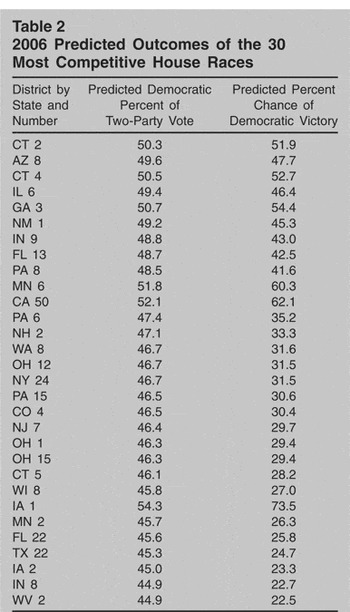
The predictions of the model for 2006 are discussed below. Unless we state otherwise, our predictions were made based on picking the “best” candidate for both parties—whenever uncertainty about what type of candidate would win a primary existed. The generally uncompetitive nature of U.S. House races documented elsewhere (Jacobson 2004) was captured by the model. It predicted that 159 races have more than a 90% chance of a Republican winning, while 199 races have more than a 90% chance of the Democrat winning. The fact that there were more such Democratic districts was also consistent with past research (Jacobson 2005). The 30 most competitive races are listed in Table 2. Many of these races had also been highlighted by the media as “races to watch.” For example, 12 of the races listed in Table 2 were listed among the top 20 races to watch by the Washington Post.7
See http://projects.washingtonpost.com/elections/keyraces/map/, accessed April 27, 2006.
www.cqpolitics.com/risk_rating_house.html, accessed April 28, 2006.
2006 Predicted Outcomes of the 30 Most Competitive House Races

The three methods of determining candidate characteristics described above were utilized for simulations of the 2006 elections. The first method included predictions based on the assumption that the “best” candidate would win each primary. The second method used predictions based on codings that were as favorable to the Republican candidates as possible. Finally, the third method used codings that were as favorable to the Democratic candidates as possible.
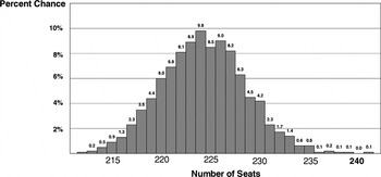
Simulations of 2,000 different elections were conducted for each of the three methods. This was done by generating normally distributed random variables, multiplying them by the standard error of the estimate for the model as a whole, and adding them to the estimated percent of the vote that Democrats would get. Districts in each simulation were then classified as either won by the Democrats, or won by the Republicans.
Figure 1 displays the probability that the Democrats would have a given number of seats after the November 2006 general election. The median estimate was that Democrats would end up with 224 seats after the election, six seats more than the party needed for control of the House. This would constitute a gain of 22 seats for the Democrats, from their current 202 seats. Overall, the model predicted that there is a 94.9% chance the Democrats will take control of the House. Ignoring the most extreme 2.5% of scenarios at the low and high end of estimates indicates that the Democrats will control between 216 and 233 seats after the election.

Chance for Number of Democratic Seats, 2006 Election
When values for 2006 non-incumbents were coded as favorably for Republicans as possible, slightly different outcomes emerged. The median estimate was that the Democrats will take 220 seats. And they were estimated to have just a 69.2% chance of taking control of the House. Ninety-five percent of the time the Democratic Party would obtain between 212 and 228 seats, under these (extremely unrealistic) assumptions. When results were coded as favorably as possible for Democrats, there was a 97.4% chance that they will take control of the House. Using these pro-Democratic assumptions, the median estimate of Democratic seats was 226. There was also a 95% chance the Democrats will win between 217 and 234 seats. These findings indicate that uncertainty about who will win primaries was not problematic for the model's predictions.
Conclusion
This article has presented a novel method of predicting House elections. Beyond that, this study has built on the foundation provided by the literature of election studies in order to identify the most important factors for predicting outcomes of congressional elections. Making use of variables that have long been studied as correlates of success in congressional elections, we predicted that the Democrats would pick up 22 seats in the November 2006 House of Representatives election. If this forecast turns out to have been correct, the election will give the Democrats 224 seats in the 435-seat House of Representatives—a 13-seat majority. We also predicted that there was a 94.9% chance that the Democrats will take control of the House.
This election forecast conflicts with other seat-by-seat analyses of the 2006 House election made immediately prior to this writing. CQ Politics called 224 seats for the Republicans. Even if the Democrats won all of the nine seats that CQ labeled “no clear favorite,” their party would be left with only 211 seats.9
See www.cqpolitics.com/, accessed April 28, 2006.
Author Bio
Carl Klarner is assistant professor of political science at Indiana State University. He holds a Ph.D. from Texas A&M University. His research interests include campaigns and elections, state politics, and welfare policy, especially as these three subjects pertain to political inequality and reform.
Stan Buchanan teaches and runs the public administration program in the department of political science at Indiana State University, Terre Haute.