


1. Introduction
The importance of history and context dependencies in decision-making processes is increasingly highlighted across a wide range of disciplines, including economics, decision theory, psychology, sociology, and law. Empirical and theoretical studies suggest that instantaneous valuations depend not only on current variables but also on past events, past decisions, and the contexts in which they occur.
In Economics, integrating the fact that “history matters” into theoretical models and into the gathering and interpretation of data on economic phenomena has become increasingly prominent in recent decades. History-dependence has long been supported in many various approaches. Models in which a representative consumer takes her past consumption as a reference point, habit-formation models, path-dependent processes, financial processes, sport or health economics, and law and economics all involve history-dependencies. These approaches emphasize that past states, actions, decisions, and contexts, whether environmental, legal, social, or institutional, influence current and future economic outcomes in different ways. History matters in the evolution of technology, institutions, agents’ behavior, inherited contexts (Guinnane et al., Reference Guinnane, Sundstrom and Whatley2003). Various applications in economics rely on the notion that history matters, including habits, path-dependence (Arrow, Reference Arrow2004; David, Reference David1997, Reference David, Garrouste and Ioannides2001; Page, Reference Page2006; Beyer, Reference Beyer2010; Gräbner-Radkowitsch and Kapeller, Reference Gräbner-Radkowitsch and Kapeller2024; Hämäläinen et al., Reference Hämäläinen and Lahtinen2016), finance (Haug, Reference Haug2001; Malmendier and Wachter, Reference Malmendier and Wachter2021), contexts and frames (Goetzmann et al. Reference Goetzmann, Watanabe and Watanabe2022; Wachter and Kahana, Reference Wachter and Kahana2024; Wendner, Reference Wendner2005), management and organizations (Marquis and Qiao, Reference Marquis and Qiao2025; Tang and Wang, Reference Tang and Wang2025), as well as technological changes coming from digital transformation (Bohnsack et al., Reference Bohnsack, Kurtz and Hanelt2021). In this literature, it can be observed that “history matters” means a wide variety of things regarding both what “history” means and how it “matters”; yet there is no consensus on what is meant by history matters in economic models. The instantaneous decision criteria crucially depend on the sequences of past events, which include, but are not restricted to, past decisions. At the same time, it still remains to be understood how the history-dependencies are formed, how such dependencies affect the decisions, and how they are affected by our decisions.
Macroeconomic variables and decisions arise and evolve within contexts. Contexts are the set of natural and cultural conditions in which organisms live and human activities take place, and they play a crucial role in many areas, whether in history, philosophy, epistemology, sociology, economics, business, law, or artificial intelligence. The evolutions of contexts and the human activities’ histories are mutually dependent. It is therefore crucial to develop frameworks that allow for the study of the various ways in which decisions and contexts interlink.
In this paper, we propose a general framework that incorporates both history-dependencies and contexts. Our framework builds upon the literature in which “history matters” signifies that, at each period, the (instantaneous) utility as well as the (current) constraints (feasible sets, budget constraints, production function) faced by agents for their decisions are influenced by the whole past history of endogenous variables and of exogenous variables.Footnote 1 Our approach is based on the introduction of a memory function, which explicitly characterizes how past events, decisions, and contexts are formed, accumulated, and transmitted over time. This formulation allows history to depend not only on past decisions but also on contextual variables and their interactions, thereby extending the scope of existing models.
History-dependencies have mainly appeared in economic models with a representative consumer taking her own past consumptions as a reference point. Axiomatically (He et al., Reference He, Dyer and Butler2019; Rozen, Reference Rozen2010; Rustichini and Siconolfi, Reference Rustichini and Siconolfi2005, Reference Rustichini and Siconolfi2014; Frick et al., Reference Frick, Iijima and Strzalecki2019), theoretically (Ryder and Heal, Reference Ryder and Heal1973; Carroll et al., Reference Carroll, Overland and Weil1997, Reference Carroll, Overland and Weil2000; Bambi and Gozzi, Reference Bambi and Gozzi2020; Bambi et al., Reference Bambi, Ghilli, Gozzi and Leocata2024; Boucekkine et al., Reference Boucekkine, Fabbri, Federico and Gozzi2022; Boucekkine et al., Reference Boucekkine, Licandro, Puch and Del Rio2005; Bambi et al., Reference Bambi, Gozzi and Licandro2014; Bambi, Reference Bambi2008; Licandro and Puch, Reference Licandro and Puch2006; Licandro et al., Reference Licandro, Puch, Ruiz, In van Montfort, Oud and Voelkle2018; Augeraud-Veron et al., Reference Augeraud-Veron, Bambi and Gozzi2017; Maille and Tuffin, Reference Maillé and Tuffin2005) and empirically (Havranek et al., Reference Havranek, Rusnak and Sokolova2017; Dynan, Reference Dynan2000; Fuhrer, Reference Fuhrer2000; Ravina, Reference Ravina2019), different viewpoints have contributed to explain some observed phenomena.Footnote 2 The literature has shown important consequences on many issues including consequences on steady states (Bossi and Gomis-Porqueras, Reference Bossi and Gomis-Porqueras2009; Wendner, Reference Wendner2002) and tax policy (Wendner, Reference Wendner2000). In this literature, a current history level is introduced, and several ways of history formation from consumptions have been considered. Consumption habit phenomena are diverse in the literature (Bambi and Gozzi, Reference Bambi and Gozzi2020; Rozen, Reference Rozen2010; Rustichini and Siconolfi, Reference Rustichini and Siconolfi2005, Reference Rustichini and Siconolfi2014; Ryder and Heal, Reference Ryder and Heal1973; Wendner, Reference Wendner2003). Wendner (Reference Wendner2003) crucially raised some fundamental issues on the very modeling. This prompted to provide results that can be derived regardless of some of the particularities of the modeling choices. Morhaim and Ulus (Reference Morhaim and Ulus2023) proposed a unified framework allowing very general consumption history formation processes, not restricted to linear cases and where utility is not restricted to additive nor multiplicative specifications, opening a path to study various history-dependencies (such as habits or satiation, but also addiction and many other effects) while providing results and dynamic programming tools to deal with these models. Such usual habit models are cases of consumption history-dependent models. These models, in which consumption history is considered, are particular cases of transforming the capital stock decisions into a history sequence. Indeed, these are cases in which consumption is kept in memory, which is a function of previous date and current capital stock decisions. It means keeping in memory a particular function of these decisions.
History-dependent phenomena in economics, nevertheless, are not all based on consumption history. The aim of this paper is to handle history-dependencies in a broader sense to tackle other history-dependencies (such as those based on investment, labor supply, research, networks) which may involve contexts such as legal norms, weather conditions, or pollution. Moreover, context and decision variables can also be mutually related. History formation processes of the reference points arise, that are not necessarily (household’s own past) consumption history formation processes and need to be conceived in a wider sense in many strands in the literature, as Wendner (Reference Wendner2005) suggested by frames. We show here that new modelings may be designed to incorporate different kinds of frames and history-dependencies. The decisions are affected by the contexts in which they occur. By our definition, contexts may be natural or cultural conditions, such as legal frameworks, social or cultural norms, environment. They thus include, but are not limited to, environmental and sustainable variables. It is important to understand, on the one hand, how history-dependencies affect the contexts, and on the other hand how history-dependencies are affected by the contexts. These two important issues are addressed in this paper, so that reconfigurations when responding to changes—whether external or internal (Goumagiasa et al., Reference Goumagias, Fernandes, Nucciarelli and Li2022)—are taken into account. On the one hand, economic models usually deal with history-dependencies formed directly through the history of past decisions or indirectly from past decision variables. What historically “matters” depends on the past decisions, but is not limited only to the past decisions themselves; it can be constituted as a function of these past decisions. On the other hand, what matters can involve different forms of history, such as those based on the past decisions themselves or on only some of the past decisions, on both past decisions and past contexts, or only past contexts (such as habit formation, path-dependence, environmental contexts). While these concepts are widely used in the literature and encompass a variety of mechanisms and interpretations, yet there is no consensus on how past experiences are generated and transmitted over time. In this paper, we address a variety of these concepts. This is achieved by introducing a “memory” function that allows us to model how history is formed, which may vary across settings, and explains how past states are formed, transformed, accumulated, and transmitted over time. To keep the formalization as simple and tractable as possible, we introduce a history sequence that allows many ways for the history to be formed as well as many ways for it to enter the valuation. This is done by explicitly modeling historical evolutions and memory formation. At each date, the instantaneous criterion depends not only on instantaneous decisions but also on the entire past history, which has been formed through a memory process. The memory function allows history to be formed through a process that is not restricted to past decisions alone but also incorporates contexts and frames. This memory function may operate directly on the model’s variables, and also explicitly determines which elements of past experience influence current decisions. These elements may consist of internal or external variables, functions of these variables, or representations derived from them.
By such means, we are able to propose a flexible approach to modeling these phenomena while keeping the tools as close as possible to those commonly used in the literature. What constitutes history is thus model-specific and is captured by our memory function, defined as a function of the relevant variables. The idea of a memory function is not new and originates in the existing literature: existing models rely on similar mechanisms but lack a unified and general framework. Our contribution in this paper is to provide a framework that unifies a wide range of existing models while remaining simple to verify and applicable to many, though not all, economic problems. In particular, our approach encompasses the large literature on consumption habits, as well as habit formation beyond consumption (e.g., environmental, financial, investment, labor supply habits), and more generally a broad class of memory effects that cannot be captured by traditional habit-based models. The flexibility of this framework thus allows us to account for various historical influences while remaining fully compatible with standard economic models. Our modeling in this paper is designed to study decisions and contexts, jointly or separately, and to allow decisions and contexts to interlink, while remaining tractable and interpretable across different settings.
An advantage of this modeling with explicit memory formation is that being very flexible, it fits standard economic models and may adapt to some new modelings (as the example of circular models shows). The framework we propose is conceived and able to take into account various kinds and widely interpretable contexts. Morhaim and Ulus (Reference Morhaim and Ulus2023) model as well as all its examplesFootnote 3 become particular cases of the history-dependent framework in this paper. It thus fits many standard models such as habit models (Rozen, Reference Rozen2010; Rustichini and Siconolfi, Reference Rustichini and Siconolfi2014; Ryder and Heal, Reference Ryder and Heal1973; Carroll et al., Reference Carroll, Overland and Weil1997, Reference Carroll, Overland and Weil2000), satiation (He et al., Reference He, Dyer and Butler2013), environmental issues and pollution (Ikefuji, Reference Ikefuji2008; Löfgren, Reference Löfgren2003; Van Der Ploeg and Withagen, Reference Van Der Ploeg and Withagen1991), optimal management of natural resource (Smulders et al., Reference Smulders, Toman and Withagen2014; Ulus, Reference Ulus, Machado, Özdemir and Baleanu2020), finance (Malmendier and Wachter, Reference Malmendier and Wachter2021; Jiang et al., Reference Jiang, Liu, Peng and Yan2025), sports (Andreff, Reference Andreff2006), and health economics (Hochli et al., Reference Höchli, Dorn, Holenweger, Messner, Schuller and Rohrbach2023; Wellsjo, Reference Wellsjo2021), sustainability issues and circular economy (CE) models (George et al., Reference George, Lin and Chen2015; Kasioumi, Reference Kasioumi2021, Reference Kasioumi2022), but also many other phenomena, as in law, legal decisions and the rule (Farber, Reference Farber2005; Lewis, Reference Lewis2021), in game theory, actions and social norms (Acemoglu and Jackson (Reference Acemoglu and Jackson2015)), in experimental economics, decision-making and social norms (Vostroknutov, Reference Vostroknutov2020), artificial intelligence, reinforcement learning (Tennenholtz et al., Reference Tennenholtz, Merlis, Shani, Mladenov and Boutilier2023). We also allow to interlink these with various kinds of effects and history-dependencies, and we consider a very general instantaneous reward function, as well as general contexts evolutions and feasible sets. Our framework in this paper also fits many environmental and sustainable models. Indeed, environmental and sustainable variables are influenced by (the memory of our past) decisions and can be treated as contexts.
Another key contribution of the paper is to show that, despite the additional complexity induced by history-dependence, it remains possible to retain the tractability of standard dynamic economic models. History-dependence introduces significant challenges, in particular because it gives rise to infinite-dimensional state variables and affects both preferences and constraints. These features complicate the application of standard optimization techniques and raise important issues regarding the existence and characterization of solutions. We address these challenges by developing optimization results and extending dynamic programming methods to the class of history-dependent models considered in this paper. At this point, dynamic programming deserves further elaboration. Dynamic programmingFootnote 4 constitutes a set of powerful methods and tools for solving a wide range of sequential decision-making problems. The idea of dynamic programming relies on the notion of equivalence between optimization problems. Two optimization problems are said to be equivalent if they have exactly the same solutions. When we face the task of finding the solutions to an optimization problem that is difficult to solve, having a method that provides an equivalent problem that is easier to solve is very useful. Such a method allows solving the equivalent problem which is easier to solve. As the method guarantees the equivalence between the two problems, we are ensured that solving the second problem gives us the solutions of the initial problem, i.e. the one of interest.
Dynamic programming allows replacing an infinite-time variables problem by a fixed-point problem with finite-time variables. It is standard in the macroeconomics literature to consider the Bellman equation as an equivalent representation of the initial problem, namely the optimization of net present value (Stokey et al., Reference Stokey, Lucas and Prescott1989; Le Van and Dana, Reference Le Van and Dana2003; Rust, Reference Rust2019).Footnote 5 However, such an equivalence holds only under certain conditions and assumptions; in particular it may fail in models with history-dependence. Ensuring the existence and uniqueness of solutions to the Bellman equation thus remains a crucial and on-going issue for macroeconomists. In the presence of history-dependencies, an additional challenge arises as infinity reappears in the very instantaneous criteria. Thus the equivalent fixed-point problem, usually with finite-time variables, here itself involves infinite-time variables. It therefore presents particular mathematical difficulties in showing that we can use these tools to solve the initial intertemporal problem. In this paper, we manage to overcome these particular mathematical difficulties. Our framework is built on easy-to-check assumptions. We establish the existence of a solution and develop dynamic programming tools that we make available. Moreover, we do so while providing a framework (including the modeling and assumptions) that is both tractable and as close as possible to standard formulations.
The paper is structured as follows. The next section is devoted to a discussion in which we handle history-dependencies in a broad sense. We then introduce the notions of history and memory formation processes. All along the section, we provide several examples to support and illustrate the discussion. This section includes a presentation of dynamic programming tools, describing how they are commonly applied to solve macroeconomic dynamics problems and under which conditions they can be used. The third section presents the model, where the standard optimization problem is presented, and history sequences, memory function, history-dependent instantaneous criteria (utility function), and constraints (feasible sets) are introduced. The results and dynamic programming tools are provided in the fourth section. All the proofs can be found in the Appendix.
2. Related literature
2.1 History-dependence
In economics, the importance of integrating the fact that history matters, in theoretical models and in the gathering and interpretation of data in economic phenomena, is widely accepted. History-dependence has long been supported in many various approaches. Models where a representative consumer takes her past consumption as a reference point, habit-formation models, path-dependent processes, financial processes, sport or health economics, and law economics, all involve history-dependencies. These approaches emphasize that past states, actions, decisions, and contexts (environmental, legal, social, institutional) influence current and future economic outcomes in different ways. History matters in the evolution of technology, institutions, agents’ behavior, inherited contexts (Guinnane et al., Reference Guinnane, Sundstrom and Whatley2003). Various applications in economics relies on the notion that history matters. These include habits, path-dependence (Arrow, Reference Arrow2004; David, Reference David1997, Reference David, Garrouste and Ioannides2001; Page, Reference Page2006; Beyer, Reference Beyer2010; Gräbner-Radkowitsch and Kapeller, Reference Gräbner-Radkowitsch and Kapeller2024; Hämäläinen et al., Reference Hämäläinen and Lahtinen2016), finance (Malmendier and Wachter, Reference Malmendier and Wachter2021), contexts and frames (Wachter and Kahana, Reference Wachter and Kahana2024; Wendner, Reference Wendner2005; Goetzmann et al., Reference Goetzmann, Watanabe and Watanabe2022), management and organizations (Marquis and Qiao, Reference Marquis and Qiao2025; Tang and Wang, Reference Tang and Wang2025), including technological changes coming from digital transformation (Bohnsack et al., Reference Bohnsack, Kurtz and Hanelt2021), etc. However, there is no consensus on what is meant by history matters in economic models (even in the “path-dependent” economic literature).
“History matters” means a variety of several various things both for what “history” means and also on how it “matters.” In this paper, “history matters” means that at each period, the (instantaneous) utility as well as the (current) constraints (feasible sets, budget constraints, production function) faced by the agents for her decision are influenced by the whole past history of endogenous variables and of exogenous variables.Footnote
6
Let us consider for example a representative consumer deriving utility from tea consumption. In the basic usual model, the instantaneous utility function
 $u$
depends on the level
 $c_t$
of tea consumption at date
 $t$
, that is
 $u(c_t)$
. But if the consumer is used to drinking tea every morning, then phenomena such as addiction, or satiation, or any possible intermediaries, variations or related effects may occur. Therefore, the instantaneous utility depends not only on her current consumption level but also on a “habit” coming from the whole past history of consumption. Thus, the utility
 $u$
at date
 $t$
depends on the current level
 $c_t$
of tea consumption but also on the history
 $\tilde {h}_t\,:\!=\,(c_{t-1},c_{t-2},\ldots \ldots )$
of consumptions preceding date
 $t$
,
 \begin{equation*} u(c_t,\tilde {h}_t) \end{equation*}
Such a habit model is a case of consumption history-dependent model. Consumption habit phenomena are diverse in the literature (Bambi and Gozzi, Reference Bambi and Gozzi2020; Rozen, Reference Rozen2010; Rustichini and Siconolfi, Reference Rustichini and Siconolfi2005, Reference Rustichini and Siconolfi2014, Ryder and Heal, Reference Ryder and Heal1973; Wendner, Reference Wendner2003). A unified framework for such consumption history-dependence that is not restricted to linear casesFootnote 7 and where utility is not restricted to additive nor multiplicative specifications was provided in Morhaim and Ulus (Reference Morhaim and Ulus2023).
Nevertheless, history-dependent phenomena in economics are not all based on consumption history. The aim of this paper is to handle history-dependencies in a broader sense to address other history-dependencies (such as based on investment, labor supply, research, networks) and which may involve contexts such as legal norms, weather conditions, pollution. Let us proceed with our previous tea consumer example and take into consideration the fact that utility coming from tea consumption also depends on the weather. Indeed, a consumer may need to consume a higher level of tea to derive the same utility when the weather gets cold.Footnote
8
Therefore, the instantaneous utility
 $u$
depends on the level
 $c_t$
of tea consumption at date
 $t$
, but also on the weather
 $w_t$
, that is
 $u(c_t,w_t)$
. Suppose there are only two weather conditions (hot
 $W_H$
or cold
 $W_C$
); to derive the same utility level, one cup of tea is needed when the weather is hot whereas three cups are needed when the weather is cold, i.e.,
 $u(1,W_H)=u(3,W_C)$
. However, to derive the same utility level today whether it is hot or cold, the number of tea cups needed today depends on the fact that it has been hot until today or it got cold for already a month. If the weather has been cold for the entire previous month, the consumer is now accustomed to the cold, and fewer cups may suffice. For clarity, when it is cold today after being cold for a month, two cups may be enough to derive a given utility level, whereas if it becomes cold today after being hot for the entire prior month, four cups may be required. That is,
 $u\big ( (2,W_C), (W_C,W_C,\ldots .,W_C)\big )=u\big ((4,W_C), (W_H,W_H,\ldots .,W_H)\big )$
. Thus, the instantaneous utility depends on the weather
 $w_t$
at date
 $t$
, but also on the entire history
 $\tilde {w}_t\,:\!=\,(w_{t-1},w_{t-2},\ldots \ldots )$
of the weather prior to date
 $t$
. That is,
 \begin{equation*} u(c_t,w_t, \tilde {w}_t). \end{equation*}
Hence, preferences depend on the history of the context, which we do not decide (it is not a consumption choice that we make). The utility
 $u$
can also depend on combined effects from consumption history and weather history
 \begin{equation*} u\big ((c_t,w_t), (\tilde {h}_t, \tilde {w}_t)\big ) \end{equation*}
Moreover, context and decision variables can be mutually related. Let us consider that the context variable
 $w_t$
is the humidity level. The humidity level
 $w_t$
at date
 $t$
is affected by the natural climate state (
 $n_t$
) and by the persistent component (
 $\gamma w_t$
). The technology process using capital (input) releases hot steam, raising humidity through capital use (
 $\theta k_t$
). Thus,
 $w_t=n_t+\gamma w_{t-1}+\theta k_t$
. The context and the input decision variables are therefore interrelated.
Furthermore, economic models usually deal with history-dependencies formed directly from the history of past decisions, or indirectly from past decision variables. Consider a representative agent deciding investment in tea so that the capital stock at date
 $t$
is
 $k_t$
. Then the decision variables are
 $k_t$
, while history-dependencies is formed through consumption
 $c_t$
, i.e. a function of
 $k_t$
and
 $k_{t+1}$
, indirectly from past decision variables
 $k_t$
.
These examples illustrate how utility depends on instantaneous decision variable (e.g.
 $c_t$
,
 $k_t$
), direct or indirect history of decision variable (
 $\tilde {h}_t$
), instantaneous context (
 $w_t$
) and history of the context (
 $\tilde {w}_t$
). In other words, history can matter either through the history of past decisions themselves, or of some of the past decisions, or through past decisions and past contexts, or only contexts. These history-dependencies extend beyond consumption history-dependence and are not captured by the framework proposed by Morhaim and Ulus (Reference Morhaim and Ulus2023). While concepts such as habit formation, path-dependence, procedure, external environment, are widely used, and encompass a variety of mechanisms and interpretations, yet there is no consensus on how past experiences are generated and transmitted over time. In this paper, we address this variety of concepts. This is achieved by introducing a “memory” function which can be different from one to another and explains how past states are formed, transformed, accumulated, and transmitted. That is, the “memory function” allows us to model the way history is formed.
What historically “matters” depends on the past decisions but is not limited to the past decisions themselves, it can be constituted of a function of these past decisions. For example, if we think in terms of instantaneous capital decisions
 $k_t$
and habits formed from consumptions, what is remembered is a function
 $f(k_t)-k_{t+1}$
of the decisions, so that we do not retain the entire sequence of past decisions but rather the entire sequence of functions of these decisions. In a model with an extracted resource in which at each date the decision consists in deciding the couple the level of stock capital and level of extraction, but in which the history-dependence comes only from extraction, the history is formed through a function of the decisions.
In financial decision models, memory plays an important role. Past crisis events can affect current decisions. Another important financial example is when choices are not based on what really happened, but based on how they are remembered (Malmendier and Wachter, Reference Malmendier and Wachter2021; Zhengyang et al., 2024). Some approaches model memory through an additional “context layer” or representation that differs from the features capturing direct experience (Wachter and Kahana, Reference Wachter and Kahana2024).
Memory is also central in Law and Economics. Legal rules, institutions, and jurisprudential concepts evolve not only in response to present conditions but through the cumulative influence of past norms and arrangements, making an intertemporal perspective essential. Contract law, for instance, develops through court decisions, as earlier cases shape how judges interpret and apply contracts, thereby influencing current expectations. Similarly, in environmental and technological contexts, including artificial intelligence, liability standards evolve through judicial and regulatory practice, with earlier decisions shaping responsibility for harms such as pollution or data misuse. In criminal law, standards of responsibility and punishment likewise develop through legislation and judicial decisions. Thus, present outcomes reflect a legal memory derived from accumulated precedents (Lacey, Reference Lacey2015; Morhaim and Ulus, Reference Morhaim and Ulus2025 and Wheatley, Reference Wheatley2021).
In sports economics, players’ investissements in themselves over time and past experiences influence their decisions on the field. Players remember patterns from past games and use them to make quick decisions. Their decisions are based on memory information about opponents, teammates, typical game situations, and changing environments, which help them act faster and more accurately (Andreff, Reference Andreff2006). Habits are sensitive to contexts, which is also a crucial issue in health economics. It is important to identify contextual, social, and personal factors that promote (benefits) and hinder (barriers) hygiene habits in care facilities (Hochli et al., Reference Höchli, Dorn, Holenweger, Messner, Schuller and Rohrbach2023; Wellsjo, Reference Wellsjo2021). For instance, if a nurse is used to washing hands in a particular setting
 $A$
and encounters another setting
 $B$
, she may not wash hands as consistently as she would have while being used to setting
 $B$
, the same nurse would have washed hands as usual. Past contexts enter the memory function, beyond the past decision variables.
Our memory function may operate directly on the variables of the model or explicitly determines which elements of past experience influence current decisions. These elements may consist of internal or external variables, functions of these variables, or representations derived from them. This flexibility allows taking into account various historical influence while remaining fully compatible with the economic structure of many specific usual models.
At each date
 $t+1$
, history is formed by augmenting the history at date
 $t$
with the elements that matter for the model, which we refer to as memory. Depending on the model, this may correspond to past consumption, extraction levels, or other relevant decision or contextual variables. What constitutes history is thus model-specific and is captured by our memory function (
 $m$
), defined as a function of the relevant variables. The idea of such a memory function is not new and comes from the existing literature: existing models rely on similar mechanisms, but lack a unified and general framework. Our contribution in this paper is to provide a framework, which unifies a wide range of existing models while remaining simple to verify and applicable to many, though not all, economic problems. In particular, our approach encompasses the large literature on consumption habits as well as habit formation beyond consumption (e.g., environmental or financial contexts), and more generally, a broad class of memory effects that cannot be captured by traditional habit-based models.
History at date
 $t$
is a sequence that consists of the whole previous history (i.e. the sequence until
 $t-1$
) completed with what just happened at the previous date
 $t-1$
. For example, in the consumption/saving optimal growth model, when decisions are considered as being the stock of capital, and when consumption habits are formed, what matters is the history of past consumptions, i.e. what completes the previous history to form the new one is the last consumption. Thus, history formation can come directly from past decisions or can come through a transformation process of past decisions. This leads to introduce a function to describe the transformation process from past decisions. We call this transformation the memory function
 $m$
. The memory function describes how the history is formed from the previous dates’ variables. In this example, at each date
 $t$
, the decision is the instantaneous capital
 $k_t$
. The history is formed from consumption history at each date
 $t$
, so history matters through the whole past sequence of consumption before
 $t$
,
 $c_t=f(k_t)-k_{t+1}$
(denoting
 $f$
the production function). History then consist not of directly the decisions
 $k_t$
but through a transformation of these decisions through calculating
 $c_t$
i.e. the function
 $f(k_t)-k_{t+1}$
. We have then
 $m(k_t,k_{t+1})=f(k_t)-k_{t+1}$
, which describes the way the history is formed from the decisions. It also encompasses cases in which history formation comes directly from the past decisions without being transformed. For example, in a model with an extracted resource in which at each date the decision consists in deciding the couple of the levels of stock capital
 $k_t$
and of the extraction rate
 $r_t$
. Suppose that the history-dependence comes only from the extraction decisions, the history is formed directly from
 $r_t$
. For such cases of direct dependence, one defines the memory function as
 $m((k_t,r_t),(k_{t+1},r_{t+1}))=r_t$
or as the identity or projection function. Suppose now that the resource that is extracted is regenerated at a rate
 $\theta$
with regeneration depending on the humidity level
 $w_t$
. The memory then depends on the context
 $w_t$
with
 $m((k_t,r_t,w_t),(k_{t+1},r_{t+1}, w_{t+1}))=r_t-\theta w_t$
. Thus, in this paper, history is formed through a memory process which is not restricted to only past decisions but which builds also upon contexts and frames.
2.2 Dynamic programming
Intertemporal economics and dynamics lead to sequential optimization problems to be solved. The theory of dynamic programming was created by Richard Bellman in the 1950s to treat the mathematical problems arising from the study of various multi-stage decision processes (Bellman, Reference Bellman1954). Dynamic programming has many concrete applications among which the earliest included management of hydroelectric reservoirs (Massé, Reference Massé1944), optimal inventory policy (Arrow et al., Reference Arrow, Harris and Marschak1951) and statistical decision rules (Wald, Reference Wald1947). Dynamic programming emerged as a fundamental tool of applied mathematics and revolutionized the way we do economics is done, being one of the most fundamental tool underlying game theory, macroeconomics, and microeconomics (see, e.g., Stokey et al., Reference Stokey, Lucas and Prescott1989; Amir et al., Reference Amir, Mirman and Perkins1991; Amir, Reference Amir1996, Adda and Cooper, Reference Adda and Cooper2003; Le Van and Dana, Reference Le Van and Dana2003; Sargent, Reference Sargent2009), so that much of the modern economics literature can be regarded as a type of applied dynamic programming (Rust, Reference Rust2019). Dynamic programming has since developed and now refers to a set of powerful methods and tools for solving a wide range of sequential decision-making.
The idea of dynamic programming relies in the notion of equivalence of optimization problems. Two problems are said to be equivalent if they have exactly the same solutions. When we face the task of finding the solutions to an optimization problem which is difficult to solve, if we have a method that provides us an equivalent problem that is easier to solve is very useful. Such a method allows solving the equivalent problem which is easier to solve. As the method guarantees the equivalence between the two problems, we are ensured that solving the second problem gives us the solutions of the initial problem which is the one that interests us.
Dynamic programming allows replacing an infinite-time variables problem by a fixed-point problem with finite-time variables. Unfortunately, this replacement is possible only for certain problems and under certain assumptions. Replacing a problem with an equivalent (i.e. having the same solutions) problem that is easier to solve is an interesting method, however, it is necessary to ensure that the new problem will yield the same solutions as the original problem. It is standard in macroeconomics literature to consider the Bellman equation as an equivalent representation of initial problem, namely the optimization of net present value (Le Van and Dana, Reference Le Van and Dana2003).Footnote 9 Nevertheless, such an equivalence does not hold always, in particular, it may not hold in models with history-dependence. Moreover, securing a unique solution to the Bellman equation is a crucial and on-going issue for macroeconomists and this can be guaranteed by adequate assumptions on the problems.
Shortly, there are conditions that need to be satisfied for a model to be fitted into a Bellman equation format. Bellman has first showed that solving certain intertemporal problems is equivalent to solving a fixed-point equation known as Bellman’s equation, and research has since extended the models that can be solved in this way. However, not all intertemporal problems can be solved this way. History-dependence introduces the fact that at each date
 $t$
, the instantaneous utility function depends on the whole the actual past events themselves, inducing problems in the possible applicability of dynamic programming tools. Here we go a step further with the possibility of history-dependence, which reintroduces infinity into the (equivalent) finite model and therefore presents particular difficulties in showing that we can use these tools to solve the initial intertemporal problem. Nevertheless, we manage to propose very simple and common assumptions that allow us to do so.
Any use of dynamic programming for intertemporal economic models thus leads to a threesome issue to be solved: providing a model that is adequate both on one hand from the economic characteristics and on the other hand from the features and assumptions that allow dynamic programming tools, i.e. conciliate economic realities and mathematical constraints, and then to develop and provide such tools. Here, there is a fourth issue to be solved when introducing history-dependent phenomena. In addition to the traditional threesome issue, the fourth issue that arises is that infinity gets back in the very instantaneous problems.
3. The model: A general history-dependent framework
According to empirical studies in many diverse areas (economics, decision theory, psychology, history, sociology, law), the instantaneous valuation depend on the instantaneous variables but referring to past events and decisions. It is crucial to be able to take this into account. For the formalization to be as simple and as manipulable as possible, we introduce a history sequence and allows many ways for the history to be formed as well as many ways it enters the valuation.
We propose a general intertemporal optimization framework in which the instantaneous reward function depends on the memory of all the previous decisions. The formalism we propose allows discussing and studying the memory process formation as well as the way the history enters the instantaneous reward function. We develop optimization results and dynamic programming tools. The very idea of Bellman’s dynamic programming tools is to replace an optimization problems depending on infinite variables by an adequate sequence of “finite” instantaneous problems. However, taking into account references to past decisions and events in the very instantaneous valuation introduces back infinity in the very instantaneous problems. Moreover, recall that Bellman’s method cannot always be used for any intertemporal problem (and therefore we cannot start by working directly on the fixed-point problem as if it were equivalent to the initial intertemporal problem); this depends on the properties of the intertemporal model. It thus requires adequate features and assumptions, hence the importance of our work. We further provide a general history-dependent framework which is both easily implementable and as general as needed to be widely applicable. This is allowed by providing a history-dependent framework in which the basic elements and premises of the problem, in particular the instantaneous reward function and the feasible set, are defined in an adequate recursive way answering both issues simultaneously. We then show that such a model is a particular case of our general history-dependent framework and the results for this particular case are derived as corollaries of the results for the general history-dependent framework.
We now detail the way we address history-dependencies.
3.1 The history-dependent instantaneous function
We describe a general framework of an infinite horizon intertemporal history-dependent decision problem of a social planner which may be a problem of optimal growth related to consumption, saving, conservation, accumulation, pollution or sustainable issues, depending on the objectives and the constraints of the model. Let us consider an intertemporal decision process. We assume that at each date
 $t$
the decision
 $x_t$
liesFootnote
10
in
 $\operatorname {I\!R}^n (n \in \operatorname {I\!N})$
. Such decisions may involve consumption decisions, investment decisions or any other economic related decisions. One example is the capital stock/saving decisions. As an illustration, let us consider the usual saving/consumption optimal growth model. In the optimal growth models, usually the instantaneous objective function
 $F$
at date
 $t$
depends on the two stock of capital variables
 $k_t$
and
 $k_{t+1}$
and is written as follows
 \begin{equation*} F(k_t,k_{t+1}) \end{equation*}
Here, the instantaneous objective function
 $F$
at date
 $t$
depends not only on the two stock of capital variables
 $k_t$
and
 $k_{t+1}$
but also on the past which is formalized through a history sequence
 $\tilde {h}_t$
, and is written as follows
 \begin{equation*} F(\tilde {h}_t, k_t,k_{t+1}) \end{equation*}
More generally, we do not restrict the model to capital stock decision variables, and we consider more general variables
 $x \in \operatorname {I\!R}^n$
so that it is written
 \begin{equation*} F(\tilde {h}_t, x_t,x_{t+1}) \end{equation*}
In the seminal habit formation literature, history consists in past consumptions sequence, i.e. it is tha particular case of consumption history-dependent model. However, the habit literature itself is enriched with other history-dependencies as technology habits, legal standards, environmental dependencies.
Let us denote
 $\mathcal{H}$
the set of all history sequencesFootnote
11
with elements in
 $\operatorname {I\!R}^p$
. That is, let us consider an agent facing a time
 $t$
objective function
 $F$
which is defined on a subset
 $\mathcal{D}_F$
of
 $\mathcal{H} \times \operatorname {I\!R}^n \times \operatorname {I\!R}^n$
 \begin{equation*} F\,:\, \mathcal{D}_F \subseteq (\mathcal{H} \times \operatorname {I\!R}^n \times \operatorname {I\!R}^n) \to \operatorname {I\!R} \end{equation*}
This framework allows studying issues and models from various literature strands. As we introduced a general function allowing to model many different memory processes, general decision variables, objective functions, and feasible sets, we are able to encompass many existing models. It generalizes the history-dependent intertemporal optimization models provided in Morhaim and Ulus (Reference Morhaim and Ulus2023). Thus, the applications presented in Morhaim and Ulus (Reference Morhaim and Ulus2023) are encompassed. These include seminal models dealing with habit formation (Rozen, Reference Rozen2010; Rustichini and Siconolfi, Reference Rustichini and Siconolfi2014; Ryder and Heal, Reference Ryder and Heal1973; Carroll et al., Reference Carroll, Overland and Weil1997, Reference Carroll, Overland and Weil2000) and satiation (He et al., Reference He, Dyer and Butler2013; Baucells and Sarin, Reference Baucells and Sarin2010). Moreover, it encompasses environmental models (Ikefuji, Reference Ikefuji2008; Löfgren, Reference Löfgren2003 and Safi and Ben Hassen Reference Safi and Hassen2021) and optimal management of natural resources (Smulders et al., Reference Smulders, Toman and Withagen2014; Ulus, Reference Ulus, Machado, Özdemir and Baleanu2020), as well as recent circular economy models (George et al., Reference George, Lin and Chen2015; Kasioumi and Stengos Reference Kasioumi and Stengos2023; Kasioumi, Reference Kasioumi2021). These existing models are particular cases of our general framework as well as how its flexibility allows using it in future research. Our general framework indeed allows studying simultaneously many effects and contexts: circular models without production waste, linear economies with production waste, and furthermore circular economies with production waste, as well as other many effects.
3.2 The memory function
We explicitely model the way history is formed using a memory function. The memory function allows treating habit-formation models (consumption history-dependance) but also many other history-dependence cases as price memory, norms, technology, legal standards, contracts. More precsiely, we define a memory function depending at each time of the last decision
 $x_{t+1}\in \operatorname {I\!R}^n$
given the previous decision
 $x_{t}$
. By this memory function
 $m$
, we will obtain the history-dependence/sequence. The memory process can induce a vector so that
 $m(x_{t},x_{t+1})$
is an element of
 $\operatorname {I\!R}^p (p \in \operatorname {I\!N})$
. Through these functions, our formalism allows studying many memory process formations and history-dependencies.
We define the memory function by
 $m\,: \operatorname {I\!R}^n \times \operatorname {I\!R}^n \to \operatorname {I\!R}^p$
such that for time
 $t$
,
 $m(x_{t}, x_{t+1})$
is the memory for the decision
 $x_{t+1}\in \operatorname {I\!R}^n$
given
 $x_{t}$
. By this memory function
 $m$
, we will obtain the history of the memories over time which is modeled in the following way. At time
 $t=0$
, she has a time-
 $0$
history denoted by
 $\tilde {h}^{(0)}\,:\!=\,(h_0^{(0)},h_1^{(0)},\ldots .)$
lying in
 $\mathcal{H}$
the set of all history sequences. Having on memory
 $m(x_0, x_1)$
at time 0, she has then time-
 $1$
history equal to
 $\tilde {h}^{(1)}\,:\!=\,(m(x_0, x_1), \tilde {h}^{(0)})$
at time
 $t=1$
. That is, by induction, for any time
 $t\geq 1$
, time-
 $t$
history will be
 \begin{equation*} \forall t\geq 1, \tilde {h}^{(t)}\,\,:\!=\,(m(x_{t-1}, x_{t}), m(x_{t-2}, x_{t-1}), \ldots .,m(x_1, x_2), m(x_0, x_1), \tilde {h}^{(0)}) \end{equation*}
The instantaneous utility function
 $F$
depends on the instantaneous decisions and on history sequence, similarly does the feasible set. The feasible correspondence
 $\Gamma \,:\, \mathcal{H} \times \operatorname {I\!R}^n \to \operatorname {I\!R}^n$
is defined such that for any
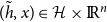 $ (\tilde {h}, x)\in \mathcal{H} \times \operatorname {I\!R}^n$
 \begin{equation*}\Gamma (\tilde {h}, x)\subseteq \{ x'\in \operatorname {I\!R}^n, (\tilde {h}, x, x')\in \mathcal{D}_F \}\end{equation*}
3.3 The problem
We now present the general intertemporal optimization framework. Let us denote
 $\tilde {x}$
the intertemporal decision sequence and
 $\mathcal{X}$
the set of all decision sequences,Footnote
12
i.e.
 \begin{equation*} \tilde {x}=(x_t)_{t=0}^{+\infty } \in \mathcal{X} \end{equation*}
Assuming a fixed discount factor
 $\beta \in (0,1)$
, for initially given state
 $x_0 \in \operatorname {I\!R}^n$
and time-
 $0$
history
 $\tilde {h}^{(0)} \in \mathcal{H}$
; with feasible state and control variables at time
 $t$
, that is, satisfying the process
 $x_{t+1} \in \Gamma (\tilde {h}^{(t)}, x_t)$
, for every
 $t\geq 0$
, the general framework optimization problem can then be written as follows:
 \begin{equation*} \left \{ \begin{array}{c@{\quad}l} \operatorname { Max } & \sum \limits _{t=0}^{+\infty } \beta ^t F\big (\tilde {h}^{(t)},x_t, x_{t+1}\big )\\ \operatorname { s.t. } & \forall t\geq 0, x_{t+1} \in \Gamma (\tilde {h}^{(t)}, x_t)\\ & \forall t \geq 1, \tilde {h}^{(t)}=(m(x_{t-1},x_{t}),\ldots ..,m(x_1,x_2),m(x_0,x_1),\tilde {h}^{(0)})\\ & x_0 \in \operatorname {I\!R}^n \operatorname { and }\ \tilde {h}^{(0)} \in \mathcal{H} \operatorname { are \ given } \end{array} \right . \end{equation*}
Although this problem is usual and useful, its lack of explicit recursivity induces implementable issues. In order to develop tools that are algorithmically computable, we will thus also consider an explicitely recursive version of the problem as follows. Let us consider
 $F \, : \operatorname {I\!R}^N \times \operatorname {I\!R}^n \times \operatorname {I\!R}^n \to \operatorname {I\!R}$
(
 $N \in \operatorname {I\!N}$
) the instantaneous reward function,
 $m \, : \operatorname {I\!R}^n \times \operatorname {I\!R}^n \to \operatorname {I\!R}^p$
the memory function and the (fixed) discount factor
 $\beta \in (0,1)$
. Let us consider an adjustement level function
 $\varphi \, : \, \mathcal{H} \to \operatorname {I\!R}^N$
, with
 $N \in \operatorname {I\!N}$
. Let
 $x_0 \in \operatorname {I\!R}^n$
and
 $\tilde {h}^{(0)} \in \mathcal{H}$
be given, and consider the problem
 \begin{equation*} \left \{ \begin{array}{c@{\quad}l} \operatorname { Maximize } & \sum \limits _{t=0}^{+\infty } \beta ^t F\big (\varphi (\tilde {h}^{(t)}), x_t, x_{t+1}\big )\\ \operatorname { s.t. } & \forall t\geq 0, x_{t+1} \in \Gamma (\tilde {h}^{(t)},x_t)\\ & \forall t \geq 1, \tilde {h}^{(t)}=(m(x_{t-1},x_{t}),\ldots ..,m(x_1,x_2),m(x_0,x_1),\tilde {h}^{(0)})\\ \end{array} \right . \end{equation*}
Recall that for any given initial data
 $x_0 \in \operatorname {I\!R}^n$
, and initial time-0 history
 $\tilde {h}^{(0)} \in \mathcal{H}$
, the feasible set
 $\Pi (\tilde {h}^{(0)},x_0)$
is defined by the set of sequences feasible from
 $x_0$
and
 $\tilde {h}^{(0)}$
, i.e. for any
 $x_0 \in \operatorname {I\!R}^n$
, for any
 $\tilde {h}^{(0)} \in \mathcal{H}$
,
 \begin{equation*} \Pi (\tilde {h}^{(0)},x_0)=\{\tilde {x}=(x_t)_{t=1}^{+\infty }\in \mathcal{X}, \forall t \geq 0, x_{t+1} \in \Gamma ( \tilde {h}^{(t)},x_t), \tilde {h}^{(t+1)}=(m(x_{t},x_{t+1}), \tilde {h}^{(t)}) \} \end{equation*}
Let us give a set
 $(\mathcal{A}')$
of assumptions: (F) on the feasible set, (A’) on the instantaneous function, and (M) on the memory function. The assumptions (F) and (M) are classical (see the details in Section 4.2).
(A’)
-
(A1’)
 $\forall x_0 \in \operatorname {I\!R}^n$
and
$\tilde {h}^{(0)} \neq 0, \exists \tilde {x} \in \Pi (\tilde {h}^{(0)},x_0)$
such that
$\sum \limits _{t=0}^{+\infty } \beta ^t F\big (\varphi (\tilde {h}^{(t)}), x_t, x_{t+1}\big ))\gt -\infty$
.
-
(A2’) The functions
$F$
and
$\varphi$
are continuous and there exist
$a \in \operatorname {I\!R}^+$
with
$a\beta \lt 1$
,
$a_2 \in \operatorname {I\!R}^+$
and a continuous function
$a_1 \,: \operatorname {I\!R}^n \rightarrow \operatorname {I\!R}$
such that for any
$x_0 \in \operatorname {I\!R}^n$
and
$\tilde {h}^{(0)} \in \mathcal{H}$
, for any feasible sequence
$\tilde {x}=(x_t)_{t=1}^{+\infty }\in \Pi (\tilde {h}^{(0)},x_0)$
and its associated history
$\tilde {h}^{(t)}$
, for any
$t\geq 0$
,
\begin{equation*} F^+(\varphi (\tilde {h}^{(t)}), x_t, x_{t+1}) \leq a_1(x_0)a^t+a_2 \end{equation*}








An easily implementable case is when the function
 $\varphi : \mathcal{H} \to \operatorname {I\!R}^N$
, with
 $N \in \operatorname {I\!N}$
can be defined recursively through a function
 $G \, : \operatorname {I\!R}^p \times \operatorname {I\!R}^N \to \operatorname {I\!R}^N$
, i.e. for any
 $\upsilon \in \operatorname {I\!R}^p$
and any
 $\tilde {h} \in \mathcal{H}$
, as
 \begin{equation*} \varphi (\upsilon ,\tilde {h})=G\big (\upsilon ,\varphi (\tilde {h}) \big ) \end{equation*}
and when the correspondence
 $\Gamma$
can be defined (and easily calculated) by
 $\varphi$
 \begin{equation*} \Gamma (\tilde {h},x)=g(\varphi (\tilde {h}),x) \end{equation*}
with
 $g \, : \operatorname {I\!R}^N \times \operatorname {I\!R}^n \to \operatorname {I\!R}^n$
is given.
The problem is then written
 \begin{equation*} \left \{ \begin{array}{c@{\quad}l} \operatorname { Maximize } & \sum \limits _{t=0}^{+\infty } \beta ^t F\big (\varphi (\tilde {h}^{(t)}), x_t, x_{t+1}\big )\\ \operatorname { s.t. } & \forall t\geq 0, x_{t+1} \in \Gamma (\tilde {h}^{(t)},x_t)\\ & \forall t \geq 1, \tilde {h}^{(t)}=(m(x_{t-1},x_{t}),\ldots ..,m(x_1,x_2),m(x_0,x_1),\tilde {h}^{(0)})\\ & \forall t \geq 1, \varphi (\tilde {h}^{(t)})=G\big (m(x_{t-1},x_{t}),\varphi (\tilde {h}^{(t-1)}) \big ) \\ & x_0 \in X \operatorname { and } \tilde {h}^{(0)} \in \mathcal{H} \operatorname { are \ given } \end{array} \right . \end{equation*}
In Morhaim and Ulus (Reference Morhaim and Ulus2023), a representative agent consumes a single good on periods
 $t=0,1,2,\ldots .$
and maximizes her intertemporal utility over the consumption stream
 $\tilde c=(c_0,c_1,\ldots .)$
. At date
 $t$
, the consumer’s instantaneous utility depends on her current consumption
 $c_t$
, and it also depends on her time-
 $t$
(consumption) history
 $\tilde {h}^{(t)}$
which is defined from an initial history
 $\tilde {h}^{(0)}$
and keeps in memory the consumption decisions. For initially given capital stock
 $k_0\gt 0$
and time-
 $0$
history
 $\tilde {h}^{(0)}$
, the general framework and optimization problem, with
 $f \, : \operatorname {I\!R}^+ \to \operatorname {I\!R}^+$
the production function,
 $k_t$
the capital stock at time
 $t$
, and
 $\beta \in (0,1)$
the fixed discount factor , is given as follows:
 \begin{equation*} \left \{ \begin{array}{c@{\quad}l} \operatorname {Maximize} & \sum \limits _{t=0}^{+\infty } \beta ^t u(c_t, \varphi (\tilde {h}^{(t)})) \\ \operatorname {s.t.} & \forall t \geq 0, k_{t+1}=f(k_t)-c_t, k_t \geq 0 \operatorname { and } c_t \geq 0 \\ & \forall t \geq 1, \tilde {h}^{(t)}=(c_{t-1},\ldots .,c_1,c_0, \tilde {h}^{(0)}) \\ \end{array} \right . \end{equation*}
The problem can be rewritten as follows:
 \begin{equation*} \left \{ \begin{array}{c@{\quad}l} \operatorname {Maximize} & \sum \limits _{t=0}^{+\infty } \beta ^t u( f(k_{t})-k_{t+1}, \varphi (\tilde {h}^{(t)})) \\ \operatorname {s.t.} & \forall t \geq 0, k_{t+1} \in [0,f(k_t)]\\ & \forall t \geq 1, \tilde {h}^{(t)}=(f(k_{t-1})-k_{t},\ldots ..,f(k_1)-k_2,f(k_0)-k_1, \tilde {h}^{(0)}) \\ \end{array} \right . \end{equation*}
This is a case in which consumption is kept in memory, which is a function of previous date and current capital stock decisions. Thus, it means keeping in memory a function of these decisions. Our general history-dependent framework allows us, not only to keep in memory the particular function defining consumption, but any function of the previous date and current decisions. By this way, the model provided in Morhaim and Ulus (Reference Morhaim and Ulus2023) as well as the models presented in Morhaim and Ulus (Reference Morhaim and Ulus2023)Footnote
13
become particular cases of our framework. Indeed, let
 $x_t=k_t\in X$
for all
 $t=0, \ldots , +\infty$
, and
 $F$
by for any
 $\tilde {h}$
and
 $x, x'$
,
 \begin{equation*} F \big (\tilde {h}, x, x' \big ) \,:\!=\, u(f(x)-x',\varphi (\tilde {h})) \end{equation*}
We define for any decision
 $x'$
given
 $x$
, the memory function/process
 $m$
by
 \begin{equation*} m(x,x')=f(x)-x' \end{equation*}
The introduction of the memory function
 $m$
to the modeling allows us to explicitly study many memory processes. Here, it is done by defining
 $m$
which associates the consumption to the capital stock decisions. History-dependence appears in various strands in the literature. Environmental economics’ models involve memory functions. For instance, Löfgren (Reference Löfgren2003)’s model and Ikefuji (Reference Ikefuji2008)’s model can be written through our framework. Löfgren (Reference Löfgren2003) proposes a model with environmental quality habit formation and in which a consumption good moreover causes a negative external effect on the environment. The social planner maximizes the utility given the negative effect of the consumption good on the environment and taking into account that there is habit formation in environmental quality. The instantaneous utility
 $u(n_t,x_t,z_t,s_t)$
depends on
 $n_t$
which is the environment that displays habit formation,
 $x_t$
the “dirty” consumption good (the environmental bad),
 $z_t$
the “clean” consumption good and
 $s_t$
the habit level related to the environment. The following relations are satisfied with
 $\gamma \in (0,1), \beta \in (0,1), \delta \in (0,1)$
,
 $y$
being an exogenously given income and
 $n$
is a given initial environment
 \begin{equation*} \left \{ \begin{array}{l} n_t=n-\gamma x_t \\ z_t=y- x_t \\ s_{t+1}=\beta n_t+(1-\delta )s_t \end{array} \right . \end{equation*}
Let
 $x_t=k_t$
for all
 $t=0\ldots \infty$
, and
 $\varphi$
is defined through the following recurrence relation, for all
 $c$
and
 $\tilde h$
,
 $ \varphi ((c,\tilde h))=\beta n+(1-\delta )\varphi (\tilde h)-\beta \gamma c$
. Let us define
 $F$
by, for any
 $\tilde {h}$
and
 $x, x'$
,
 \begin{equation*} F \big (\tilde {h}, x, x' \big ) \,:\!=\,u(n-\gamma (f(x)-x'),f(x)-x',y-(f(x)-x'),\varphi (\tilde {h})) \end{equation*}
In this model, the memory function
 $m$
is defined by
 $m(x,x')=f(x)-x'$
. Thus, Löfgren (Reference Löfgren2003)’s model is encompassed in our general framework. Ikefuji (Reference Ikefuji2008) studies habit formation in consumption and pollution abatement activities when agents derive disutility both from the habit stock and pollution. The pollution
 $P_t$
in period
 $t$
is generated by the capital stock
 $k_t$
used in production and reduced by abatement activities
 $a_t$
in the same period. The problem is written as follows.
 \begin{equation*} \left \{ \begin{array}{c@{\quad}l} \operatorname { Max } & \sum \limits _{t=0}^{+\infty } \beta ^t u(c_t,H_t,P_t)\\ \operatorname { s.t. } & \forall t \geq 1, H_{t+1}=\rho c_t+(1-\rho )H_t \operatorname { and } P_t=\bigg (\dfrac {k_t}{a_t}\bigg )^{\phi }\\ & \forall t \geq 0, k_{t+1}=Ak_t-c_t-a_t-k_t \\ & k_0\gt 0, m_0\gt 0 \operatorname { and } h_0 \operatorname { are }\ \operatorname { given } \end{array} \right . \end{equation*}
where
 $c_t$
denotes the consumption in period
 $t$
,
 $H_t$
denotes the consumption habit, and
 $P_t$
is the level of aggregated pollution in the economy. This problem is covered by our framework, let
 $x_t=(k_t,a_t)$
for all
 $t=0\ldots \infty$
and the function
 $\varphi$
be defined by
 $\varphi (\tilde {h}^{(0)})=h_0$
and for all
 $\tilde {h}$
and
 $c$
,
 $\varphi (c, \tilde {h})=G (c, \varphi (\tilde {h}))$
, with the function
 $G$
defined by
 $G(c,y)=\rho c+(1-\rho )y$
. Also, the function
 $F$
is
 $F \big (\tilde {h}, x, x' \big ) \,:\!=\, u\big (f(\pi _1(x))-\pi _1(x'),\varphi (\tilde {h}), \big (\frac {\pi _1(x)}{\pi _2(x)}\big )^{\phi }\big )$
using the
 $i$
-th projections. For any decision
 $x'$
given
 $x$
, the memory function is defined by
 $m(x,x')=f(\pi _1(x))-\pi _1(x')$
. These two examples illustrate how our framework is general and easy to use, while keeping the environmental effects to be studied visible and interpretable. Our framework is also fitted to optimal management of natural resources. Smulders et al. (Reference Smulders, Toman and Withagen2014) and Ulus (Reference Ulus, Machado, Özdemir and Baleanu2020) present models referring to the optimal management of exhaustible natural resources like oil, coal, gas. In these models, there exists a single planner who manages the decision of extraction and consumption of an exhaustible natural resource at each period
 $t$
in order to maximize the intertemporal utility. At each period
 $t$
, the instantaneous utility depends on its consumption
 $c_t$
and also on the stock of the natural resource, which is denoted by
 $s_t$
. The output
 $y_t\in \operatorname {I\!R}_{+}$
is produced from capital (
 $k_t$
) and extracted quantity of resource (
 $r_t$
) (or the extraction flow of natural resource per unit of time) by a production function
 $f \, : \operatorname {I\!R}_{+}\times \operatorname {I\!R}_{+} \to \operatorname {I\!R}_{+}$
where
 $y_t = f(k_t, r_t)$
. The output is either consumed as
 $c_t\geq 0$
or saved as capital to the next period as
 $k_{t+1}$
satisfying
 $c_t + k_{t+1}\leq f(k_t, r_t) + (1-\delta )k_t \hbox{ with } k_t\geq 0$
, where
 $\delta$
stands for the depreciation rate of capital. For initially given stocks of
 $k_0, s_0, r_0\gt 0$
and
 $\beta \in (0,1)$
the fixed discount factor, assuming that
 $u$
is increasing with respect to
 $c$
, the problem of the planner can be given as follows:
 \begin{equation*} \left \{ \begin{array}{c@{\quad}l} \operatorname {Maximize} & \sum \limits _{t=0}^{+\infty } \beta ^t u(c_t,s_t) \\ \operatorname {s.t.} & \forall t \geq 0, s_{t+1} = s_t-r_t \\ & \forall t \geq 0, 0 \leq c_t=f(k_t,r_t)+(1-\delta ) k_t-k_{t+1} \\ & s_0,k_0, r_0\gt 0 \operatorname { are }\ \operatorname { given }\\ \end{array} \right . \end{equation*}
which can be rewritten as
 \begin{equation*} \left \{ \begin{array}{c@{\quad}l} \operatorname {Maximize} & \sum \limits _{t=0}^{+\infty } \beta ^t u(f(k_t,r_t)+(1-\delta ) k_t-k_{t+1}, s_t) \\ \operatorname {s.t.} & \forall t \geq 0, s_{t+1} = s_t-r_t \\ & \forall t \geq 0, 0 \leq k_{t+1} \leq f(k_t,r_t)+(1-\delta ) k_t \\ & s_0,k_0, r_0\gt 0 \operatorname { are }\ \operatorname { given }\\ \end{array} \right . \end{equation*}
Let us define
 $G$
by
 $G(s,r)\,:\!=\,s-r$
and
 $\varphi$
by the law of motion
 $\varphi (\tilde {h}^{(t+1)})=G(r_t,\varphi (\tilde {h}^{(t)}))$
for all
 $t \geq 0$
, so that the instantaneous utility
 $u(c_t, s_t)$
is
 $u(c_t,\varphi (\tilde {h}^{(t)}))$
. By defining
 $\tilde {h}^{(0)}$
such that
 $\varphi (\tilde {h}^{(0)})=s_0$
and for any
 $t \geq 0$
,
 $\tilde {h}^{(t+1)}$
such that
 $\tilde {h}^{(t+1)}=(r_t, \tilde {h}^{(t)})$
, the model can be written
 \begin{equation*} \left \{ \begin{array}{c@{\quad}l} \operatorname {Maximize} & \sum \limits _{t=0}^{+\infty } \beta ^t u( f(k_t,r_t)+(1-\delta ) k_t-k_{t+1}, \varphi (\tilde {h}^{(t)})) \\ \operatorname {s.t.} & \forall t \geq 0, k_{t+1} \in [0, f(k_t,r_t)+(1-\delta ) k_t]\\ & \forall t \geq 0, \tilde {h}^{(t+1)}=(r_{t}, \ldots .,\tilde {h}^{(0)}) \\ \end{array} \right . \end{equation*}
The model is written in our general framework by defining
 $x=(k,r)$
, the memory function by
 $m(x,x')=\pi _2(x)$
, the utility by
 $F(x,x', \tilde {h})=u \big ( f(\pi _1(x),\pi _2(x))+(1-\delta ) \pi _1(x)-\pi _1(x'), \varphi (\tilde {h}) \big )$
and the feasible set by
 $\Gamma (\tilde {h},x)=\{ x', 0 \leq \pi _1(x') \leq f(\pi _1(x),\pi _2(x))+(1-\delta ) \pi _1(x), 0 \leq \pi _2(x') \leq \varphi ( \tilde {h}) \}$
. The function
 $G$
is defined by
 $G(s,r)\,:\!=\,s-r$
. Note also that our framework allows considering more general forms of
 $G$
, for example if it comes to taking into account the resources regeneration (whether naturally or otherwise).
All these previous examples involved linear economies. Our framework deals further with the new circular economies models. Circular economy is most frequently depicted as a combination of reduce, reuse and recycle activities (Kirchherr et al., Reference Kirchherr, Yang, Schulze-Spüntrup, Heerink and Hartley2023), but also design, implying a focus on the entire life cycle of the processes as well as the interaction between the process and the environment and the economy in which it is embedded (Ghisellini, et al. Reference Ghisellini, Cialani and Ulgiati2016). The circular economy models provided by George et al. (Reference George, Lin and Chen2015), Kasioumi and Stengos (Reference Kasioumi and Stengos2022), Kasioumi (Reference Kasioumi2022) can be written in our framework, and this for the circular economy models without recycling habits (George et al., Reference George, Lin and Chen2015 and Kasioumi and Stengos, Reference Kasioumi and Stengos2023) as well as the circular economy models with recycling habits (Kasioumi (Reference Kasioumi2021)).
Our framework encompasses circular models without recycling habits proposed by George et al. (Reference George, Lin and Chen2015), and Kasioumi and Stengos (Reference Kasioumi and Stengos2023). George et al. (Reference George, Lin and Chen2015) and Kasioumi and Stengos (Reference Kasioumi and Stengos2023) consider a closed economy with zero population growth. They abstract from capital accumulation and technical progress.Footnote
14
The social planner maximizes an intertemporal utility where the instantaneous utility
 $u(c,P)$
depends on consumption
 $c$
and the stock of pollution
 $P$
. The output is produced via a (concave) production function
 $\phi$
using two factors of production, one which corresponds to the rate of use of the recyclable resource and another (
 $z$
) corresponding to the rate of use of the environmentally polluting resource. Output produced in any given period but not consumed or used for the employment of the polluting resource, accumulates as (potentially recyclable) waste. Recycling turns waste into a useful factor of production: a proportion
 $b$
of the waste stock
 $s$
with intensity of recycling
 $\tau$
is supposed to be recycled each period. George et al. (Reference George, Lin and Chen2015)’s model is a particular case of Kasioumi and Stengos (Reference Kasioumi and Stengos2023) in which the intensity of recycling
 $\tau$
is equal to one. The social planner solves the following optimization problem
 \begin{equation*} \left \{ \begin{array}{c@{\quad}l} \operatorname {Maximize} & \sum \limits _{t=0}^{+\infty } \beta ^t u(c_t,p_t) \\ \operatorname {s.t.} & \forall t \geq 0, s_{t+1}-s_t=\phi (\tau bs_t,z_t)-c_t-\alpha z_{t+1}-\tau b s_t \\ & \forall t \geq 0, p_{t+1}-p_t=\theta z_t -\delta p_t+(1-b) s_t\\ & s_0,z_0\gt 0, p_0 \geq 0 \operatorname { are }\ \operatorname { given }\\ \end{array} \right . \end{equation*}
Our memory function
 $m$
allows displaying the fact that at each date
 $t$
,
 $p_{t+1}$
depends on the previous pollution stock
 $p_t$
and of
 $[\theta z_t +(1-b) s_t]$
, in other words,
 $p_{t+1}$
depends on the memory of
 $[\theta z_t +(1-b) s_t]$
, analagously as in Ryder and Heal (Reference Ryder and Heal1973)
 $h_{t+1}$
depends on the previous habit level
 $h_t$
and of
 $c_t=f(x_t)-x_{t+1}$
, that is
 $h_{t+1}$
depends on the memory of consumptions
 $c_t=f(x_t)-x_{t+1}$
. For the model by George et al. (Reference George, Lin and Chen2015), we define
 $x=(s,z)$
, and
 $m(x,x')=\theta z +(1-b) s=\theta \pi _2(x) +(1-b) \pi _1(x)$
, and
 $G(m(x,x'),p)=(1-\delta ) p + m(x,x')$
. This modeling allows us to highlight the economic processes at work: on one hand the memory process, i.e. in George et al. (Reference George, Lin and Chen2015) how the decisions
 $x,x'$
are transformed into additional pollution, and on the other hand how this new additional pollution combines with the previous pollution state to form the new one (through
 $G$
). Kasioumi (Reference Kasioumi2021) extends this model by both incorporating habit formation on recycling and a (given) intensity
 $\tau$
of recycling. The circular models with recycling habits proposed by Kasioumi (Reference Kasioumi2021, Reference Kasioumi2022) are also encompassed by our framework. It is an extension of the theoretical work of Kasioumi and Stengos (Reference Kasioumi and Stengos2023), combining elements of the circular economy model of George et al. (Reference George, Lin and Chen2015) with the habit formation framework of Ikefuji (Reference Ikefuji2008). Kasioumi (Reference Kasioumi2021, Reference Kasioumi2022) deals with a fixed intensity of recycling while Kasioumi (Reference Kasioumi2022) deals further with an intensity
 $\tau (H_t)$
depending (through an affine function
 $\tau (H_t)\,:\!=\,\eta +rH_t$
) on the level of recycling habits. These models (Kasioumi, Reference Kasioumi2021) fit our framework. Note that our framework fits also recycling intensity functions
 $\tau$
that are not necessarily affine.
4. Dynamic programming tools
4.1 Notations and feasible sets
Definition 4.1.
For any given initial data
 $x_0 \in \operatorname {I\!R}^n$
, and initial time-0 history
 $\tilde {h}^{(0)} \in \mathcal{H}$
, the feasible set
 $\Pi (x_0,\tilde {h}^{(0)})$
is defined by the set of sequences feasible from
 $x_0$
and
 $\tilde {h}^{(0)}$
, i.e. for any
 $x_0 \in \operatorname {I\!R}^n$
, for any
 $\tilde {h}^{(0)} \in \mathcal{H}$
,
 \begin{equation*} \Pi (\tilde {h}^{(0)},x_0)=\{\tilde {x}=(x_t)_{t=1}^{+\infty }\in \mathcal{X}, \forall t \geq 0, x_{t+1} \in \Gamma ( \tilde {h}^{(t)},x_t), \tilde {h}^{(t+1)}=(m(x_{t},x_{t+1}), \tilde {h}^{(t)}) \} \end{equation*}
The process is analogous as usual. The feasible set is defined from
 $x_0$
but here also from the given (infinite) sequence
 $\tilde {h}^{(0)}$
. Once
 $x_1$
is chosen in the feasible set
 $\Gamma ( \tilde {h}^{(0)}, x_0)$
, the sequence
 $\tilde {h}^{(1)}$
is updated from the current chosen variable
 $x_1$
and the given variable
 $x_0$
. Then,
 $x_2$
is chosen given
 $x_1$
and
 $\tilde {h}^{(1)}$
in the feasible set
 $\Gamma (\tilde {h}^{(1)}, x_1)$
. And so on, at time
 $t+1$
, given
 $x_t$
and
 $\tilde {h}^{(t)}$
, the variable
 $x_{t+1}$
must be chosen in the feasible set
 $\Gamma (\tilde {h}^{(t)},x_t)$
. Once
 $x_{t+1}$
is chosen, at time
 $t+2$
,
 $x_{t+2}$
is chosen given
 $x_{t+1}$
and
 $\tilde {h}^{(t+1)}$
that has been updated from the previous history sequence
 $\tilde {h}^{(t)}$
and the variables
 $(x_t,x_{t+1})$
. Such a process allows us to keep decisions in memory while choosing the variable
 $x_t$
at each time
 $t$
.
For a sequence
 $\tilde {x}=(x_t)_{t=1}^{+\infty } \in \Pi (\tilde {h}^{(0)},x_0)$
, we denote by
 $\mathcal{U}(\tilde {x})$
the objective
 \begin{equation*} \mathcal{U}(\tilde {x})=\sum \limits _{t=0}^{+\infty } \beta ^t F(\tilde {h}^{(t)}, x_t, x_{t+1}) \end{equation*}
4.2 Assumptions
We set that
 $(F,\Gamma )$
satisfies the list
 $(\mathcal{A})$
of assumptions if the following assumptions (F) on the feasible set, (A) on the instantaneous function, and (M) on the memory function are satisfied.
(F)
(F1)
 $\Gamma$
is a continuous nonempty compact-valued correspondence from
 $\mathcal{H} \times \operatorname {I\!R}^n$
into
 $\operatorname {I\!R}^n$
.
(F2) There exists
 $a \geq 0, a \neq 1$
and
 $a' \geq 0$
such that for any
 $x \in \operatorname {I\!R}^n$
and any history
 $\tilde {h} \in \mathcal{H}$
,
 $x' \in \Gamma (\tilde {h},x) \Rightarrow \Vert x' \Vert \leq a \Vert x \Vert + a'$
(A)
(A1)
 $\forall x_0 \in X$
and
 $\tilde {h}^{(0)} \neq 0, \exists \tilde {x} \in \Pi (\tilde {h}^{(0)},x_0)$
such that
 $\mathcal{U}(\tilde {x})\gt -\infty$
.
(A2) The function
 $F$
is continuous and there exist
 $a \in \operatorname {I\!R}^+$
with
 $a\beta \lt 1$
,
 $a_2 \in \operatorname {I\!R}^+$
and a continuous function
 $a_1 \, : \, X \rightarrow \operatorname {I\!R}^+$
such that for any
 $x_0 \in \operatorname {I\!R}^n$
and
 $\tilde {h}^{(0)} \in \mathcal{H}$
, for any feasible sequence
 $\tilde {x}=(x_t)_{t=1}^{+\infty }\in \Pi (\tilde {h}^{(0)},x_0)$
and its associated history
 $\tilde {h}^{(t)}$
, for any
 $t\geq 0$
,
 \begin{equation*} F^+(\tilde {h}^{(t)}, x_t, x_{t+1}) \leq a_1(x_0)a^t+a_2 \end{equation*}
where
 $F^+(\tilde {h}, x, x') =\sup \{F(\tilde {h}, x, x'),0\}$
. (M) The function
 $m$
is continuous.
The next result shows that, under the set of assumptions
 $(\mathcal{A})$
, the objective function of the optimization problem is well-defined. Moreover, whe show the existence of a solution to the optimization problem. The uniqueness is obtained under additional assumptions, requiring strict concavity of the instantaneous function
 $F$
. We give these results in a general framework, in particular without any differentiability assumptions. The strict joint concavity of
 $F$
allows us to guarantee uniqueness. The proofs are given in the Appendix.
Proposition 4.1.
Assume
 $(\mathcal{A})$
and let
 $x_0 \in \operatorname {I\!R}^n$
and
 $\tilde {h}^{(0)} \in \mathcal{H}$
be given. Then
-
(i) for any feasible sequence
$ \tilde {x}=(x_t)_{t=1}^{+\infty }\in \Pi (\tilde {h}^{(0)},x_0)$
, the limit
$\lim _{T \rightarrow +\infty }\sum \nolimits _{t=0}^{T} \beta ^t F\big (\tilde {h}^{(t)},$
$x_t, x_{t+1}\big )$
is well-defined, where for all
$t \geq 1,$
$\tilde {h}^{(t)}=(m(x_{t-1},x_{t}),m(x_{t-2},x_{t-1}),\ldots ..,$
$m(x_1,x_2),m(x_0,x_1),\tilde {h}^{(0)})$
. -
(ii) Assume also that
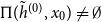
$\Pi (\tilde {h}^{(0)}, x_0) \neq \emptyset$
. Then there exists an optimal solution. If moreover
$F$
is jointly strictly concave in
$(y,x,x')$
on
$\mathcal{H} \times \operatorname {I\!R}^n \times \operatorname {I\!R}^n$
, then the solution is unique.








4.3 The value function and the Bellman equation
We now define the value function of the optimization problem. We show that under the set of assumptions
 $(\mathcal{A})$
, dynamic programming tools can be used to study our problem. We first study the properties of the value function. We then provide an appropriate set of functions on which the Bellman operator has a unique fixed point which is the value function.
Definition 4.2.
The value function
 $V$
is defined on
 $\mathcal{H} \times \operatorname {I\!R}^n$
by for any
 $(\tilde {h}^{(0)},x_0) \in \mathcal{H} \times \operatorname {I\!R}^n$
 \begin{equation*} V(\tilde {h}^{(0)},x_0)=\left \{ \begin{array}{c@{\quad}l} \operatorname { Max } & \sum \limits _{t=0}^{+\infty } \beta ^t F(\tilde {h}^{(t)}, x_t, x_{t+1})\\ \operatorname { s.t. } & \forall t\geq 0, x_{t+1} \in \Gamma (\tilde {h}^{(t)},x_t)\\ & \forall t \geq 1, \tilde {h}^{(t)}=(m(x_{t-1},x_{t}),\ldots ..,m(x_1,x_2),m(x_0,x_1),\tilde {h}^{(0)})\\ & \tilde {h}^{(0)} \in \mathcal{H} \ {and}\ x_0 \in \operatorname {I\!R}^n \ { are } \ {given} \end{array} \right . \end{equation*}
The next proposition states some further properties on the value function. These properties, together with the upper semi-continuity, will provide an appropriate set of functions to consider for dynamic programming tools.
Proposition 4.2.
Assume
 $(\mathcal{A})$
. Then
-
(a) the value function
$V$
is upper semi-continuous.
-
(b) the value function
$V$
satisfies
-
(i)
$\forall x_0,\tilde {h}^{(0)}, \tilde {x} \in \Pi (\tilde {h}^{(0)},x_0), \overline{\lim} _{t \rightarrow +\infty } \beta ^t V(\tilde {h}^{(t)},x_t) \leq 0$
. -
(ii)
$\forall x_0, \tilde {h}^{(0)}$
,
$\forall \tilde {x} \in \Pi (\tilde {h}^{(0)},x_0)$
such that
$\mathcal{U}( \tilde {x})\gt -\infty$
,
$\lim \nolimits _{t \rightarrow +\infty } \beta ^t V(\tilde {h}^{(t)},x_t)=0$
.
-




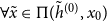


The proof of this proposition can be found in the Appendix. A standard proof (see Theorem 4.4 p.75 Stokey et al., Reference Stokey, Lucas and Prescott1989) allows us to show the following result.
Proposition 4.3.
Assume
 $(\mathcal{A})$
. Then
 $\tilde {x}^*$
is an optimal solution if and only if
 \begin{equation*} \forall t \geq 0, V(\tilde {h}^{* (t)},x_{t}^*)=F(\tilde {h}^{* (t)}, x_{t}^*,x_{t+1}^*)+\beta V(\tilde {h}^{* (t+1)},x_{t+1}^*) \end{equation*}
where
 $\tilde {h}^{* (t)}=(m(x_{t-1}^*,x_{t}^*),m(x_{t-2}^*,x_{t-1}^*),\ldots ..,m(x_1^*,x_2^*),m(x_0^*,x_1^*),\tilde {h}^{(0)})$
4.4 The value function is the unique fixed-point of the Bellman operator
Let
 $B$
be the Bellman operator, i.e.
 $B \,: \, \mathcal{F}(\mathcal{H} \times \operatorname {I\!R}^n,\operatorname {I\!R}) \rightarrow \mathcal{F}(\mathcal{H} \times \operatorname {I\!R}^n,\operatorname {I\!R})$
be defined byFootnote
15
 \begin{equation*} \forall w \in \mathcal{F}(\mathcal{H} \times \operatorname {I\!R}^n,\operatorname {I\!R}), Bw(\tilde {h},x)=\max \limits _{x' \in \Gamma (\tilde {h},x)} \{ F(\tilde {h},x,x')+\beta w((m(x,x'),\tilde {h}), x') \} \end{equation*}
Definition 4.3.
Let
 $\mathcal{F}_{b}(\mathcal{H} \times \operatorname {I\!R}^n,\operatorname {I\!R})$
be the set of upper semi-continuous functions
 $w \in \mathcal{F}(\mathcal{H} \times \operatorname {I\!R}^n,\operatorname {I\!R})$
such that
-
(i)
$\forall x_0 \in X, \forall \tilde {x} \in \Pi (\tilde {h}^{(0)},x_0), \mathop{\overline{\lim}}\nolimits _{t \rightarrow +\infty } \beta ^t w(\tilde {h}^{(t)},x_t) \leq 0$
, with
$\tilde {h}^{(t)}=(m(x_{t-1},x_{t}),m(x_{t-2},$
$x_{t-1}),\ldots ..,m(x_1,x_2),m(x_0,x_1),\tilde {h}^{(0)})$
-
(ii)
$\forall x_0, \forall \tilde {x} \in \Pi (\tilde {h}^{(0)},x_0)$
with
$\mathcal{U}(\tilde {x}) \gt -\infty$
, one has
$\lim \nolimits _{t \rightarrow +\infty } \beta ^t w(\tilde {h}^{(t)},x_t)=0.$






We now finally state that the value function is the unique fixed-point of the Bellman operator on this set of functions. The proof is given in Appendix.
Proposition 4.4.
Assume
 $(\mathcal{A})$
. Then the value function
 $V$
is the unique fixed-point of the Bellman operator on the set of functions
 $\mathcal{F}_{b}(\mathcal{H} \times \operatorname {I\!R}^n,\operatorname {I\!R})$
.
Finally, this shows that dynamic programming tools can be used to deal with general history-dependent optimal growth models.
4.5 Dynamic programming tools for the particular cases with an adjustment level function
The following optimization results and dynamic programming tools are then derived as corollaries of the ones previously shown for the general history-dependent model. Assume
 $(\mathcal{A}')$
in this subsection hereafter.
Corollary 4.1.
Assume
 $(\mathcal{A'})$
. The problem with an adjustment level function is well-defined. Assume moreover that
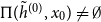 $\Pi (\tilde {h}^{(0)},x_0) \neq \emptyset$
. Then there exists an optimal solution. Moreover, if
 $F$
is jointly strictly concave in
 $(y,x,x')$
on
 $\mathcal{H} \times \operatorname {I\!R}^n \times \operatorname {I\!R}^n$
and
 $\varphi$
is linear, then the solution is unique.
Definition 4.4.
The value function
 $V$
is defined on
 $\mathcal{H}\times \operatorname {I\!R}^n$
by for any
 $(\tilde {h}^{(0)},x_0) \in \mathcal{H} \times \operatorname {I\!R}^n$
 \begin{equation*} V(\tilde {h}^{(0)},x_0)=\left \{ \begin{array}{c@{\quad}l} \operatorname { Max } & \sum \limits _{t=0}^{+\infty } \beta ^t F(\varphi (\tilde {h}^{(t)}), x_t, x_{t+1})\\ \operatorname { s.t. } & \forall t\geq 0, x_{t+1} \in \Gamma (\tilde {h}^{(t)},x_t)\\ & \forall t \geq 1, \tilde {h}^{(t)}=(m(x_{t-1},x_{t}),\ldots ..,m(x_1,x_2),m(x_0,x_1),\tilde {h}^{(0)})\\ & \tilde {h}^{(0)} \in \mathcal{H} \ {and}\ x_0 \in \operatorname {I\!R}^n \ {are} \ {given} \end{array} \right . \end{equation*}
We further define (see Appendix for the details) an appropriate set of functions
 $\mathcal{F}_{b}(\mathcal{H} \times \operatorname {I\!R}^n,\operatorname {I\!R})$
for which dynamic programming tools can be derived. All the (mathematical) details are given in the Appendix.
Let
 $B$
be the Bellman operator, i.e.
 $B \, : \, \mathcal{F}(\mathcal{H} \times \operatorname {I\!R}^n,\operatorname {I\!R}) \rightarrow \mathcal{F}(\mathcal{H} \times \operatorname {I\!R}^n,\operatorname {I\!R})$
be defined by
 \begin{equation*} \begin{array}{ll} \forall w \in \mathcal{F}(\mathcal{H} \times \operatorname {I\!R}^n,\operatorname {I\!R}), Bw(\tilde {h},x) & =\max \limits _{x' \in \Gamma (\tilde {h},x)} \{ F(\varphi (\tilde {h}),x,x')+\beta w((m(x,x'),\tilde {h}), x') \} \\ & =\max \limits _{x' \in g(\varphi (\tilde {h}),x)} \{ F(\varphi (\tilde {h}),x,x')+\beta w((m(x,x'),\tilde {h}), x') \} \end{array} \end{equation*}
Corollary 4.2.
Assume
 $(\mathcal{A'})$
. Then the value function
 $V$
is the unique fixed-point of the Bellman operator on the set of functions
 $\mathcal{F}_{b}(\mathcal{H} \times \operatorname {I\!R}^n,\operatorname {I\!R})$
.
5. Conclusion
In this paper, we develop a general and flexible intertemporal framework for dynamic macroeconomic models that incorporates history and context dependencies. By introducing a memory function, we provide a tractable and unified way to capture a broad class of history-dependent preferences, constraints, and environments. This modeling strategy encompasses several existing approaches in the literature, including habit-formation models based on consumption or other economic variables, as well as applications in decision theory, health economics, sports economics, financial economics, environmental economics, and law and economics, while also extending to some new models such as those in circular economy.
From a methodological perspective, we establish key optimization results. We develop the dynamic programming tools tailored to this class of models. In particular, we show that the value function exists and is the unique fixed point of the Bellman operator. We thus show that the standard machinery can still be applied directly despite the specific difficulties induced by history-dependence. More precisely, by introducing a flexible memory function together with the associated dynamic programming tools, we provide a set of mathematical results that can be applied in different settings for analyzing interdependencies between contexts and decisions across domains as discussed in the paper (including habit-formation models, based on consumption or other economic variables, legal dynamics), and toward many others, such as formal models of legal evolution, game-theoretic models of norms (Acemoglu and Jackson, Reference Acemoglu and Jackson2015), experimental and behavioral economics (Vostroknutov, Reference Vostroknutov2020), and reinforcement learning in artificial intelligence (Tennenholtz et al., Reference Tennenholtz, Merlis, Shani, Mladenov and Boutilier2023). This framework provides a basis for future work aiming to incorporate and analyze various forms of history-dependence within and across these fields.
These results ensure that standard dynamic programming techniques can be directly applied within this enriched, history-dependent setting, thereby offering a solid foundation for future research.
Acknowledgement
This work was supported by the French Cooperation with Galatasaray University Consortium (Thematic Project 2023–2024: Society and Culture: Decision and Transitions) and also by the Galatasaray University Research Grant Number FBA-2024-1206. We are grateful to Rabah Amir for useful discussions and comments during this work. We thank Manjira Datta, Kevin Reffett and Juan-Pablo Rincon Zapatero for having outreached important questions about this work. We also thank Luciano de Castro, Jean-Pierre Drugeon, Dominika Machowska, Antoine Le Riche, Agnieszka Wiszniewska-Matyszkiel, Lucasz Wozny, and the participants to SAET 2023 and PET 2024. Also a special thank for interesting exchanges with Ay¸se Sevencan; the members of CRED; Youcef Askoura, Antoine Billot, Sandra Cavaco, Chantal Marlats, Lucie M´enager and the LEMMA Seminar participants; Philippe Bich, Jean-Marc Bonnisseau, Pascal Gourdel, Bernard de Meyer and Agnieszka Rusinowska at CES; J´er´emie Cabessa, Yann Strozecki and the participants to the DAVID-Universit´e Versailles-Saint-Quentin Seminar.
Appendix A
A.1 Proof of Proposition 4.1
-
(i) By the assumption
$(\mathcal{A})$
, along a feasible path
$\tilde {x}=(x_t)_{t=1}^{+\infty }\in \Pi (x_0,\tilde {h}^{(0)})$
, with associated history
$\tilde {h}^{(t)}=(m(x_{t-1},x_{t}),m(x_{t-2},x_{t-1}),\ldots ..,m(x_1,x_2),m(x_0,x_1),\tilde {h}^{(0)})$
,Then for all
\begin{equation*} \forall t, F(\tilde {h}^{(t)}, x_t, x_{t+1}) \leq a_1(x_0)a^t+a_2 \end{equation*}
$T \in \operatorname {I\!N}$
,since
\begin{equation*} \begin{array}{ll} \sum \limits _{t=0}^{T} \beta ^t F(\tilde {h}^{(t)}, x_t, x_{t+1}) & \leq \sum \limits _{t=0}^{T} \beta ^t(a_1(x_0)a^t+a_2) \\ & = a_1(x_0)\sum \limits _{t=0}^{T} (a\beta )^t+a_2\sum \limits _{t=0}^{T} \beta ^t \end{array} \end{equation*}
$0\lt a\beta \lt 1$
and
$0\lt \beta \lt 1$
the conclusion follows.
-
(ii) Let us show that the objective is upper semi-continuous and the feasible sequence set is a compact set of the product topology. By (F), one can check by induction that for any given
$x_0 \in \operatorname {I\!R}^n$
and
$\tilde {h}^{(0)} \in \mathcal{H}$
, for all feasible sequence
$\tilde {x}=(x_t)_t \in \Pi (\tilde {h}^{(0)},x_0)$
, for all
$t, x_{t+1} \in \Gamma ( \tilde {h}^{(t)},x_t)$
, we haveThe feasible set
\begin{equation*} \forall t, \Vert x_t \Vert \leq a^t \Vert x_0 \Vert +\frac {1-a^t}{1-a}a'=\left(\Vert x_0 \Vert -\frac {a'}{1-a}\right)a^t+\frac {a'}{1-a} \end{equation*}
$\Pi (\tilde {h}^{(0)},x_0)$
is included in a compact set for the product topology. Moreover, it is closed. So the feasible set
$\Pi (\tilde {h}^{(0)},x_0)$
is also compact.









We next show that the objective function
 $\mathcal{U}$
is upper semi-continuous.
Let us consider a sequence
 $\tilde {x}^n=\{(x_t^n)_{t=1}^{+\infty }\}_n \subset \Pi (\tilde {h}^{(0)},x_0)$
that converges to
 $\tilde {x}=(x_t)_{t=1}^{+\infty } \in \Pi (\tilde {h}^{(0)},x_0)$
. Note that when
 $n$
converges to
 $+\infty$
, by (M), the sequence of associated histories
 $\forall t {\geq} 1, \widetilde {h^n}^{(t)}=(m(x_{t-1}^n,x_{t})^n,\ldots ..,m(x_0^n,x_1^n),\tilde {h}^{(0)})$
converges to the associated history
 ${\forall t \geq 1}, \tilde {h}^{(t)}=(m(x_{t-1},x_{t}),\ldots ..,m(x_0,x_1),\tilde {h}^{(0)})$
.
Let us show that
 $\mathop{\overline{\lim}}\nolimits _{n \rightarrow +\infty }\mathcal{U}(\tilde {x}^n) \leq \mathcal{U}(\tilde {x})$
. The notation
 $\mathop{\overline{\lim}}$
means
 $\lim \sup$
.
For any
 $t \geq 0$
, by (A2), for any
 $\tilde {x}=(x_t)_{t=1}^{+\infty } \in \Pi (\tilde {h}^{(0)},x_0)$
and with history
 $\tilde {h}^{(t)}$
associated to
 $\tilde {x}$
 \begin{equation*} F^+(\tilde {h}^{(t)}, x_t, x_{t+1}) \leq a_1(x_0)a^t+a_2 \end{equation*}
and by
 $0\lt a\beta \lt 1$
, for any
 $\varepsilon \gt 0$
, there exists
 $T_\varepsilon$
such that for any
 $(x_t)_{t=1}^{+\infty } \in \Pi (\tilde {h}^{(0)},x_0)$
, and for any
 $T\geq T_\varepsilon$
,
 \begin{equation*} \sum \limits _{t=T}^{+\infty } \beta ^t F^+(\tilde {h}^{(t)}, x_t, x_{t+1}) \leq \varepsilon \end{equation*}
So for any
 $\varepsilon \gt 0$
, there exists
 $T_\varepsilon$
such that for any
 $n \in \operatorname {I\!N}$
and for any
 $T\geq T_\varepsilon$
,
 \begin{equation*} \sum \limits _{t=T}^{+\infty } \beta ^t F^+(\widetilde {h^n}^{(t)}, x_t^n, x_{t+1}^n) \leq \varepsilon \end{equation*}
and for any
 $n \in \operatorname {I\!N}$
and for any
 $T\geq T_\varepsilon$
,
 \begin{equation*} \begin{array}{ll} \sum \limits _{t=0}^{+\infty } \beta ^t F(\widetilde {h^n}^{(t)}, x_t^n, x_{t+1}^n) & = \sum \limits _{t=0}^{T} \beta ^t F(\widetilde {h^n}^{(t)}, x_t^n, x_{t+1}^n)+ \sum \limits _{t=T}^{+\infty } \beta ^t F(\widetilde {h^n}^{(t)}, x_t^n, x_{t+1}^n)\\ & \leq \sum \limits _{t=0}^{T} \beta ^t F(\widetilde {h^n}^{(t)}, x_t^n, x_{t+1}^n)+ \sum \limits _{t=T}^{+\infty } \beta ^t F^+(\widetilde {h^n}^{(t)}, x_t^n, x_{t+1}^n)\\ & \leq \sum \limits _{t=0}^{T} \beta ^t F(\widetilde {h^n}^{(t)}, x_t^n, x_{t+1}^n)+\varepsilon \end{array} \end{equation*}
By taking
 $n \rightarrow +\infty$
(and using the continuity of
 $F$
in the right-hand side of the above inequality),
 \begin{equation*} \mathop{\overline{\lim}}\limits _{n \rightarrow +\infty } \sum \limits _{t=0}^{+\infty } \beta ^t F(\widetilde {h^n}^{(t)}, x_t^n, x_{t+1}^n) \leq \sum \limits _{t=0}^{T} \beta ^t F(\tilde {h}^{(t)}, x_t, x_{t+1})+\varepsilon \end{equation*}
Since this is true for any
 $T\geq T_\varepsilon$
, by taking
 $T\rightarrow +\infty$
,
 \begin{equation*} \mathop{\overline{\lim}}\limits _{n \rightarrow +\infty } \sum \limits _{t=0}^{+\infty } \beta ^t F(\widetilde {h^n}^{(t)}, x_t^n, x_{t+1}^n) \leq \sum \limits _{t=0}^{+\infty } \beta ^t F(\tilde {h}^{(t)}, x_t, x_{t+1})+\varepsilon \end{equation*}
Since this is true for any
 $\varepsilon \gt 0$
, by taking
 $\varepsilon \rightarrow 0$
,
 \begin{equation*} \mathop{\overline{\lim}}\limits _{n \rightarrow +\infty } \sum \limits _{t=0}^{+\infty } \beta ^t F(\widetilde {h^n}^{(t)}, x_t^n, x_{t+1}^n) \leq \sum \limits _{t=0}^{+\infty } \beta ^t F(\tilde {h}^{(t)}, x_t, x_{t+1}) \end{equation*}
So
 $\mathcal{U}$
is upper semi-continuous on
 $\Pi (\tilde {h}^{(0)},x_0)$
.
By Weierstrass Theorem (Aubin (Reference Aubin1994), Theorem 5.3.1), since
 $\mathcal{U}$
is upper semi-continuous and
 $\Pi (\tilde {h}^{(0)},x_0)$
is a compact set for the product topology, there exists an optimal solution.
The assumptions that
 $F$
is jointly strictly concave ensures the uniqueness of the solution.
A.2 Proof of Proposition 4.2
(a) A direct proof using (A2) can be done. Indeed, let us consider a sequence
 $(\widetilde {h^n}^{(0)},x_0^n)_n \subset \mathcal{H} \times \operatorname {I\!R}^n$
that converges to
 $(\tilde {h}^{(0)}, x_0) \in \mathcal{H} \times \operatorname {I\!R}^n$
, use the fact that
 $x_0^n$
converges to
 $x_0$
and let us consider a subsequence
 $(\widetilde {h^{n_i}}^{(0)}, x_0^{n_i})_i$
such that
 \begin{equation*} \mathop{\overline{\lim}}\limits _{n \rightarrow +\infty } V(\widetilde {h^n}^{(0)},x_0^n)=\lim \limits _{i \rightarrow +\infty } V(\widetilde {h^{n_i}}^{(0)},x_0^{n_i}) \end{equation*}
Let
 $\varepsilon \gt 0$
. By (A2), there exist
 $i_0$
and
 $T_0$
such that for any
 $i \geq i_0$
and for any
 $T \geq T_0$
, and for optimal path
 $({\tilde {x}}^{n_i})_i \in \Pi (\widetilde {h^{n_i}}^{(0)},x_0^{n_i})$
and its associated history
 $\widetilde {h^{n_i}}^{(t)}$
,
 \begin{equation*} V(\widetilde {h^{n_i}}^{(0)},x_0^{n_i})=\sum \limits _{t=0}^{+\infty } \beta ^t F(\widetilde {h^{n_i}}^{(t)}, x_t^{n_i}, x_{t+1}^{n_i}) \leq \sum \limits _{t=0}^{T} \beta ^t F(\widetilde {h^{n_i}}^{(t)}, x_t^{n_i}, x_{t+1}^{n_i})+\varepsilon \end{equation*}
Fix
 $T \geq T_0$
. The subsequence
 $({\tilde {x}}^{n_i})_i$
that belongsFootnote
16
to
 $\Pi (\widetilde {h^{n_i}}^{(0)}, x_0^{n_i})$
can be assumed to converge to some
 $\tilde {x}$
in
 $\Pi (\tilde {h}^{(0)},x_0)$
. By the definition of the associated history and the continuity of
 $m$
, this implies that
 $(\widetilde {h^{n_i}}^{(t)})_i$
converges to
 $\tilde {h}^{(t)}$
the history associated to
 $\tilde {x}$
.
Let
 $i \rightarrow +\infty$
, by the continuity of
 $F$
,
 \begin{equation*} \mathop{\overline{\lim}}\limits _{n \rightarrow +\infty } V(\widetilde {h^n}^{(0)},x_0^n) \leq \sum \limits _{t=0}^{T} \beta ^t F(\tilde {h}^{(t)}, x_t, x_{t+1})+\varepsilon \end{equation*}
Let
 $T \rightarrow +\infty$
,
 \begin{equation*} \mathop{\overline{\lim}}\limits _{n \rightarrow +\infty } V(\widetilde {h^n}^{(0)},x_0^n) \leq \mathcal{U}(\tilde {x})+\varepsilon \leq V(\tilde {h}^{(0)},x_0) \end{equation*}
by the arbitrariness of
 $\varepsilon$
.
(b) One can check (see Le Van and Morhaim, Reference Le Van and Morhaim2002) that (F2) and (A) imply that
(H)
 $\forall x_0 \in X, \exists \mathcal{V}(x_0)$
a compact neighborhood of
 $x_0$
in
 $X$
,
 $\forall \varepsilon \gt 0, \exists T_0$
such that
 $\forall T \geq T_0, \forall x'_0 \in \mathcal{V}(x_0), \forall \tilde {x}' \in \Pi (\tilde {h}^{(0)},x'_0)$
, one has with
 $\tilde {h}'^{(t)}=(m(x'_{t-1},x'_{t}),m(x'_{t-2},x'_{t-1}),\ldots ..,$
 $m(x'_1,x'_2),m(x'_0,x'_1),\tilde {h}^{(0)})$
,
 \begin{equation*} \sum \limits _{t=T}^{+\infty } \beta ^t F^+(\tilde {h}'^{(t)}, x'_t, x'_{t+1}) \leq \varepsilon \end{equation*}
where
 $F^+(h,r,r')=\max \{0,F(h,r,r')\}$
.
-
(i) By (H),
$\exists T_0, \forall T\gt T_0, \forall x'_0 \in \mathcal{V}(x_0), \varepsilon \gt 0, \forall \tilde {x}' \in \Pi (\tilde {h}^{(0)},x_0)$
,Let
\begin{equation*} \sum \limits _{t=T}^{+\infty } \beta ^t F(\tilde {h}'^{(t)}, x'_t, x'_{t+1}) \leq \sum \limits _{t=T}^{+\infty } \beta ^t F^+(\tilde {h}'^{(t)}, x'_t, x'_{t+1}) \leq \varepsilon \end{equation*}
$\tilde {x}' \in \Pi (\tilde {h}^{(0)},x'_0), T \geq T_0$
. For any
$\tilde {x}''=(x''_{T+1},\ldots .) \in \Pi (\tilde {h}'^{(T)},x'_T)$
, one has
$(x'_1,\ldots .,x'_T, x''_{T+1},\ldots .) \in \Pi (\tilde {h}^{(0)},x'_0)$
, andso
\begin{equation*} \beta ^T F(\tilde {h}'^{(T)}, x'_T, x''_{T+1})+\beta ^{T+1} F(\tilde {h}'^{(T+1)}, x''_{T+1}, x''_{T+2})+\ldots . \leq \varepsilon \end{equation*}
$\beta ^T V(\tilde {h}^{(T)}, x'_T) \leq \varepsilon$
which implies
$(i)$
.
-
(ii)
$\forall \tilde {x} \in \Pi (\tilde {h}^{(0)}, x_0)$
,and
\begin{equation*} - \infty \lt \mathcal{U}(\tilde {x}) \leq \sum \limits _{t=0}^{T} \beta ^t F(\tilde {h}^{(t)},x_t, x_{t+1}) +\beta ^{T+1} V(\tilde {h}^{(T+1)},x_{T+1}) \end{equation*}
The notation
\begin{equation*} 0=\lim \limits _{T \rightarrow +\infty } [\mathcal{U}(\tilde {x})-\sum \limits _{t=0}^{T} \beta ^t F(\tilde {h}^{(t)},x_t, x_{t+1})] \leq \mathop{\underline{\lim}} \limits _{T \rightarrow +\infty } \beta ^{T+1} V(\tilde {h}^{(T+1)}, x_{T+1}) \end{equation*}
$\underline{\lim}$
means
$\lim \inf$
. From
$(i)$
then
$\lim _{T \rightarrow +\infty } \beta ^{T+1} V(\tilde {h}^{(T+1)}, x_{T+1})=0$
.








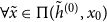



A.3 Proof of Proposition 4.4
The proof that
 $V$
is a fixed-point of the Bellman operator is standard (see Stokey et al., Reference Stokey, Lucas and Prescott1989). Uniqueness of the fixed point is shown by contradiction. Indeed, suppose there exists
 $W$
another fixed-point of
 $\mathcal{B}$
in
 $\mathcal{F}_{b}(\mathcal{H} \times \operatorname {I\!R}^n,\operatorname {I\!R})$
. Let us first check that
 $W \leq V$
. Let
 $(\tilde {h}^{(0)},x_0)$
be given. There exists
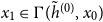 $x_1 \in \Gamma (\tilde {h}^{(0)}, x_0)$
such that
 $W(\tilde {h}^{(0)},x_0) = F(\tilde {h}^{(0)},x_0,k_1)+ \beta W(\tilde {h}^{(1)},x_1)$
and by induction, there exists a sequence
 $(x_t)_{t \geq 1}$
with associated history sequence
 $(\tilde {h}^{(t)})_t$
such that for any
 $T$
,
 \begin{equation*} W(\tilde {h}^{(0)}, x_0)=\sum \limits _{t=0}^{T-1} \beta ^t F(\tilde {h}^{(t)},x_{t},x_{t+1})+ \beta ^T W(\tilde {h}^{(T)}, x_T) \end{equation*}
Since
 $W$
belongs to
 $\mathcal{F}_{b}(\mathcal{H} \times \operatorname {I\!R}^n,\operatorname {I\!R})$
, one has taking the limit when
 $T \rightarrow +\infty$
, and then by
 $V$
being the sup of the sum
 \begin{equation*} W(\tilde {h}^{(0)},x_0) \leq \sum \limits _{t=0}^{+\infty } \beta ^t F(\tilde {h}^{(t)},x_{t},x_{t+1}) \leq V(x_0,\tilde {h}^{(0)}) \end{equation*}
Let us now show that
 $V \leq W$
. Let
 $x_0 \in X, \tilde {h}^{(0)} \in \mathcal{H}$
. For any
 $\tilde {x} \in \Pi (\tilde {h}^{(0)},x_0)$
such that
 $\mathcal{U}(\tilde {x}) \gt -\infty$
, one has, with
 $\tilde {h}^{(1)}=(m(x_0,x_1), \tilde {h}^{(0)})$
,
 \begin{equation*} \begin{array}{ll} W(\tilde {h}^{(0)},x_0) & =BW(\tilde {h}^{(0)},x_0) \\ & \geq F(\tilde {h}^{(0)},x_0,x_1)+\beta W((m(x_0,x_1), \tilde {h}^{(0)})), x_1) \\ & = F(\tilde {h}^{(0)},x_0,x_1)+\beta W(\tilde {h}^{(1)}, x_1) \\ \end{array} \end{equation*}
and so by induction, with
 $\tilde {h}^{(t)}=(m(x_{t-1},x_{t}),\ldots ..,m(x_0,x_1), \tilde {h}^{(0)})$
,
 \begin{equation*} \begin{array}{l@{\quad}l} W(x_0, \tilde {h}^{(0)}) & \geq \sum \limits _{t=0}^{T} \beta ^t F(\tilde {h}^{(t)},x_{t},x_{t+1})+\beta ^{T+1} W(\tilde {h}^{(T+1)},x_{T+1}) \\ & \geq \lim \limits _{T \rightarrow +\infty } \sum \limits _{t=0}^{T}\beta ^t F(\tilde {h}^{(t)},x_{t},x_{t+1})+ \lim \limits _{T \rightarrow +\infty } \beta ^{T+1} W(\tilde {h}^{(T+1)}, x_{T+1}) \\ & = \mathcal{U}(\tilde {x}) \end{array} \end{equation*}
which implies that
 $W(\tilde {h}^{(0)},x_0) \geq V(\tilde {h}^{(0)},x_0)$
(since for any
 $\tilde {x} \in \Pi (\tilde {h}^{(0)},x_0)$
, one has
 $W(\tilde {h}^{(0)},x_0) \geq \mathcal{U}(\tilde {x})$
and
 $V(\tilde {h}^{(0)},x_0)$
is the sup of
 $\mathcal{U}(\tilde {x})$
for
 $\tilde {x}$
in
 $\Pi (\tilde {h}^{(0)},x_0)$
).
Finally, this shows that dynamic programming tools can be used to deal with general history-dependent optimal growth models.





