


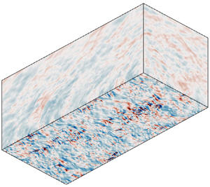



1. Introduction
Shedding light on the physics of pressure fluctuations in a compressible turbulent boundary layer (TBL) is of great significance for theoretical turbulence modelling, where the fluctuating pressure is important in redistributing the turbulent kinetic energy (Pope Reference Pope2000). Besides, it is also important for relevant engineering applications. The fluctuating pressure on aerodynamic surfaces is responsible for vibrational loading as well. In the case of high-speed vehicles, surfaces subjected to fluctuating pressure for a long time would face the risk of structural fatigue (Bull Reference Bull1996). To advance turbulence modelling and engineering design, a thorough understanding of the nature of pressure fluctuations is highly desirable.
To date, extensive efforts have been devoted to investigating TBLs, and some fundamental understanding of pressure fluctuations has been obtained. Theoretically, Lilley (Reference Lilley1963) extended the work of Phillips (Reference Phillips1960) and developed a theory of wall pressure fluctuations involving the effects of compressibility. They showed that fluctuating pressure results from fluctuations in both the vorticity mode and the acoustic mode. Typically, the former component is considered to be dominant within the TBL, whereas the latter is dominant in the free stream in the form of an eddy Mach wave, but the roles played by these two modes in various layers of a TBL for different parameters require investigation. In experiments, directly measuring global pressure fluctuations lacks practice so far. Thus, existing measurements have focused on pressure fluctuations in the free stream and at the wall surface. Laufer (Reference Laufer1964) provided some important experimental results for the acoustic fluctuations in the free stream with free-stream Mach number  $M_\infty$ up to 5. Kistler & Chen (Reference Kistler and Chen1963) firstly measured the wall pressure fluctuations beneath supersonic TBLs over the Mach number range
 $M_\infty =1.33$–
 $5$. They reported the intensities of pressure fluctuations, space–time correlations as well as convection speed and found the major effect of increasing the Mach number is to decrease the length scale of the pressure field. Then, a large amount of experimental data (Maestrello Reference Maestrello1969; Tan, Tran & Bogdonoff Reference Tan, Tran and Bogdonoff1987; Beresh et al. Reference Beresh, Henfling, Spillers and Pruett2011) have been obtained, and significant scatter emerged among these nominally compatible experimental results, especially for the magnitudes of wall pressure fluctuations. Surface-mounted pressure transducers were used in these experiments, and thus fluctuating wall pressure signals were obtained in a certain average sense. As a result, Dolling & Dussauge (Reference Dolling and Dussauge1989) and Beresh et al. (Reference Beresh, Henfling, Spillers and Pruett2011) have argued that the reliability of these measurements of the variance and frequency spectra of wall pressure fluctuations is in doubt. Accurate and global data on fluctuating pressure are desired for understanding the mechanism of pressure fluctuations and turbulence modelling. Recently, complementary to experiments, direct numerical simulation (DNS) has become a powerful tool due to its capability of providing access to physical quantities that are difficult to obtain experimentally. Nonetheless, it is restricted to relatively low Reynolds numbers. Bernardini, Pirozzoli & Grasso (Reference Bernardini, Pirozzoli and Grasso2011) took the lead in performing DNS of supersonic TBLs to study the wall pressure with
 $M_\infty =2,3,4$. They demonstrated the effects of varying the Reynolds number and Mach number on the wall pressure signature from a series of DNSs in the supersonic regime. Duan, Choudhari & Wu (Reference Duan, Choudhari and Wu2014) used DNS to examine the pressure fluctuations generated by a TBL of
 $M_\infty =2.5$, with a focus on pressure fluctuations within the TBL and the acoustics in the near field. Generally, DNS is regarded as a very suitable method to explore the nature of pressure fluctuations because it can provide accurate and global data on flow fields. However, detailed DNS studies focusing on pressure fluctuations covering subsonic to hypersonic regimes are still rare.
In practice, a wall with a temperature lower than that of the adiabatic wall is frequently encountered due to considerable radiative cooling and internal heat transfer, such as in high-speed vehicles and tunnel nozzles. The heat transfer between the TBL flow and the wall surface can modify the statistical properties of the TBL significantly (Duan, Beekman & Martín Reference Duan, Beekman and Martín2010; Chu, Zhuang & Lu Reference Chu, Zhuang and Lu2013; Hadjadj et al. Reference Hadjadj, Ben-Nasr, Shadloo and Chaudhuri2015; Zhang, Duan & Choudhari Reference Zhang, Duan and Choudhari2018). It is of great practical significance to investigate the wall-cooling effect on the physics of flow structures, pressure fluctuations and their corresponding modelling. Duan et al. (Reference Duan, Beekman and Martín2010) performed DNSs of Mach 5 TBLs with wall-to-edge temperature ratios from 1.0 to 5.4. With wall cooling effects, they found compressibility effects are enhanced but remain insignificant, and the coherency of turbulent structures is also increased. Many scaling relations that are used to express statistics of adiabatic compressible TBLs also hold for non-adiabatic cases. Hadjadj et al. (Reference Hadjadj, Ben-Nasr, Shadloo and Chaudhuri2015) used large-eddy simulation to study the role of wall temperature in the mean and fluctuating-flow properties of Mach 2 TBLs. An adiabatic wall case and two cold wall cases were considered, by which compressible skin friction was found to be higher for cold wall TBLs than adiabatic TBLs. Zhang et al. (Reference Zhang, Duan and Choudhari2018) established DNS databases for supersonic and hypersonic TBLs with Mach numbers ranging from 2.5 to 14 and wall-to-recovery temperature ratios  $T_w/T_r$ ranging from 0.18 to 1.0 to gauge the performance of compressibility transformations. Nevertheless, they paid less attention to the wall-cooling effect on pressure fluctuations. Duan, Choudhari & Zhang (Reference Duan, Choudhari and Zhang2016) numerically examined the pressure fluctuations generated by a spatially developed Mach 5.86 TBL with
 $T_w/T_r=0.76$, thus providing the first-ever comparison of mean-velocity profiles and surface pressure spectrum with experimental measurements at hypersonic Mach number. Then, Zhang, Duan & Choudhari (Reference Zhang, Duan and Choudhari2017) conducted a DNS at a lower ratio of
 $T_w/T_r=0.25$ with the same Mach number. Combining these two databases, they showed that near-wall pressure fluctuation intensities and the frequency spectrum of wall pressure fluctuations are dramatically modified by wall temperature conditions. However, in supersonic or subsonic regimes, the effect of wall cooling on pressure fluctuations has rarely been discussed. In order to better understand the mechanism, a systematic study of the wall-cooling effect in regimes of different Mach number is required.
To discriminate the generating mechanisms of pressure fluctuations, the pressure Poisson equation is usually employed in wall-bounded flows, which can provide more physical insight originating from governing equations. For incompressible flow, the Poisson equation gives two primary source terms, which contribute to the two major components of pressure fluctuations, namely the rapid pressure corresponding to the interactions between mean velocity gradients and turbulence and the slow pressure corresponding to turbulence–turbulence interactions (Pope Reference Pope2000). As observed in an incompressible channel flow, Kim (Reference Kim1989) found that the slow pressure fluctuations are stronger than the rapid pressure fluctuations throughout the channel except very near the wall, where they are about the same magnitude. Chang, Piomelli & Blake (Reference Chang, Piomelli and Blake1999) studied the contributions of the two pressure components in wavenumber space, and the dominating contributions of sources in the buffer region in most of the wavenumber range were highlighted. Gerolymos, Sénéchal & Vallet (Reference Gerolymos, Sénéchal and Vallet2013) extended the decomposition such that the pressure is separated into not only rapid and slow parts but also volume and surface terms. They placed emphasis on the wall echo effects on pressure fluctuations. Recently, Anantharamu & Mahesh (Reference Anantharamu and Mahesh2020) analysed these two wall pressure fluctuation sources in combination with spectral proper orthogonal decomposition. Foysi, Sarkar & Friedrich (Reference Foysi, Sarkar and Friedrich2004) extended the Poisson-equation-based method to compressible channel flow to study the pressure–strain correlation. Very recently, Tang et al. (Reference Tang, Zhao, Wan and Liu2020) and Yu, Xu & Pirozzoli (Reference Yu, Xu and Pirozzoli2020) split the pressure fluctuations in compressible channel flows and demonstrated the importance of the additional pressure part corresponding to compressibility effects at high Mach numbers. Despite this, existing works on pressure decomposition are primarily focused on turbulent channel flows which are easy to implement as both streamwise and spanwise directions are considered periodic and homogeneous, and the patterns of the pressure components in compressible TBLs have never been reported.
The goal of this study is to explore the general effects of wall cooling on pressure fluctuations in zero-pressure-gradient compressible TBLs at various compressibility intensities. A series of DNSs of  $M_\infty =0.5$, 2.0 and 8.0 TBLs with quasi-adiabatic wall and their cooled-wall counterparts have been performed. Because the pressure fluctuations are closely related to the vorticity mode and acoustic mode, the turbulence statistics, such as vorticity and dilatation fluctuations, turbulent Mach numbers and the instantaneous flow structures are compared to show the effects of wall cooling intuitively. The characteristics of pressure fluctuations versus Mach numbers are also compared with the existing empirical model. To reveal the mechanisms of modifications on pressure fluctuations by wall cooling, we extend the method of the pressure decomposition to compressible TBL flows with the aid of the acoustic radiation feature in the free stream. The pressure fluctuations are decomposed into five components corresponding to different generating mechanisms, and their characteristics and contributions of each pressure component are illustrated in detail.
The remainder of the paper is organized as follows. The numerical methods and simulation details are outlined in § 2 and the general turbulence statistics of boundary layers are given in § 3. Section 4 shows the modifications of wall cooling on flow structures. Then § 5 is focused on a discussion of the pressure fluctuation fields. Section 6 introduces the process of the pressure decomposition and reveals corresponding pressure components. Finally, the main findings are summarized in § 7.
2. Numerical methods and simulation details
Direct numerical simulations are performed for zero-pressure-gradient TBLs with an isothermal wall. The three-dimensional Navier–Stokes equations for a compressible, viscous, perfect heat-conducting gas are solved in a stretched Cartesian coordinate system by high-order finite-difference methods. The temperature-dependent coefficient of viscosity  $\mu$ is calculated using Sutherland's law. The simulations are based on the open-source code STREAmS released by Bernardini et al. (Reference Bernardini, Modesti, Salvadore and Pirozzoli2021), which can be accelerated by graphics processing units. A brief review of the numerical methods of STREAmS used in the present work is introduced here. The spatial discretization of the convective terms in the Navier–Stokes equations is based on a hybrid energy-preserving/shock-capturing scheme in a locally conservative form. In smooth (shock-free) regions of the flow, the convective flux is approximated by the eighth-order energy-preserving scheme (Pirozzoli Reference Pirozzoli2010). Otherwise, in the discontinuous regions, the Lax–Friedrichs flux vector splitting ensures robust shock-capturing capabilities. The seventh-order weighted essentially non-oscillatory reconstruction (Jiang & Shu Reference Jiang and Shu1996) is utilized to reconstruct the components of positive and negative characteristic fluxes at interfaces. To determine the switch between the energy-preserving and shock-capturing discretizations, a modified version of the Ducros shock sensor is used (Ducros et al. Reference Ducros, Ferrand, Nicoud, Weber, Darracq, Gacherieu and Poinsot1999). The viscous terms are expanded to Laplacian form to avoid odd–even decoupling phenomena and are approximated with the sixth-order central finite-difference formulas. For time integration, the semi-discrete system assembled from the discretization of the spatial derivatives is advanced in time using a three-stage, third-order Runge–Kutta scheme (Spalart, Moser & Rogers Reference Spalart, Moser and Rogers1991). More details of the numerical methods can be found in Bernardini et al. (Reference Bernardini, Modesti, Salvadore and Pirozzoli2021).
A schematic of the computational model is shown in figure 1. A fully developed turbulent state is established by the recycling–rescaling procedure (Pirozzoli, Bernardini & Grasso Reference Pirozzoli, Bernardini and Grasso2010), which is less noisy than a synthetic inflow like the digital filtering method. At the upper and outflow boundaries, non-reflecting boundary conditions (Poinsot & Lele Reference Poinsot and Lele1992) are imposed based on characteristic decomposition in the direction normal to the boundary. A similar characteristic wave treatment is also applied at the no-slip isothermal wall boundary. Uniform grid spacing is used in the spanwise direction, and hyperbolic sine stretching is applied in the wall-normal direction. The grid spacing is uniform in the streamwise direction except at the end of the computational domain where stretching is applied. A sponge zone (Adams Reference Adams1998) in combination with grid stretching is added surrounding the computational domain at the top and the tail to further eliminate reflections. The reference state of the flow in the sponge zone is set as the mean flow.
A sketch of the computational model (not to scale). The bottom plane denotes the isothermal wall. Location  $x_r$ indicates the streamwise location of the recycling domain. The computational domain is surrounded by the sponge zone at the top and the tail.

The computational cases and simulation parameters are listed in table 1. Six DNSs have been performed in three different Mach number regimes, including three quasi-adiabatic cases whose isothermal wall temperature  $T_w$ is set to the recovery temperature
 $T_{r}=T_{\infty }(1+r(\gamma -1) M_{\infty }^{2} / 2)$ based on a recovery factor of
 $r=0.89$, and three corresponding cooled-wall counterparts. At the stations selected for analysis, the friction Reynolds number is chosen as
 $Re_\tau \approx 650$, which is defined as the ratio between the boundary layer thickness
 $\delta$ and the wall viscous length scale
 $\delta _{v}=\bar {\nu }_{w} / u_{\tau }$, where
 $u_{\tau }=\sqrt {\tau _{w} / \bar {\rho }_{w}}$ is the friction velocity,
 $\bar {\rho }_{w}$ is the mean density at the wall,
 ${\tau }_{w}$ is the mean wall shear stress and
 ${\nu }_{w}$ is the kinematic viscosity. It is worth noting that the variation of thermodynamic properties across compressible non-adiabatic boundary layers is large. Thus a single Reynolds number is not sufficient to characterize the flow (Lele Reference Lele1994). The choice of a more appropriate Reynolds number to compare flows at different Mach numbers is a matter of controversy (Smits & Dussauge Reference Smits and Dussauge2006). Whereas the near-wall pressure signature and flow structures we are interested in are subjected to the boundary layer state in the inner layer, we choose the friction Reynolds number
 $Re_\tau$ as a suitable similarity parameter, which is the same as in previous works (Bernardini & Pirozzoli Reference Bernardini and Pirozzoli2011; Hadjadj et al. Reference Hadjadj, Ben-Nasr, Shadloo and Chaudhuri2015; Zhang et al. Reference Zhang, Duan and Choudhari2017, Reference Zhang, Duan and Choudhari2018). The free-stream temperature of the
 $M_\infty =8.0$ cases refers to the condition of nozzle exit of the Sandia Hypersonic Wind Tunnel at Mach 8 (Zhang et al. Reference Zhang, Duan and Choudhari2018). The inflow is of low enthalpy such that the real gas effect is absent.
The computation cases and simulation parameters. Here  $M_\infty$,
 $Re_\infty$ and
 $T_\infty$ are the free-stream Mach number, Reynolds number and temperature, respectively;
 $Re_\tau$ is the friction Reynolds number;
 $T_w/T_r$ means the ratio of isothermal wall temperature and recovery temperature;
 $T_w/T_e$ means the ratio of isothermal wall temperature and boundary edge temperature; and
 $\delta _i$ is the inlet boundary layer thickness.

The spatial and temporal settings of simulations are listed in table 2. The grid resolutions are evaluated at the streamwise station where  $Re_\tau \approx 650$. Due to the high-resolution capability of the hybrid eighth-order energy-preserving and seventh-order weighted essentially non-oscillatory scheme, the present grid resolutions are sufficient for DNS. A higher resolution is achieved in the
 $M_\infty =8.0$ cases to capture finer turbulent eddies. The sponge zones are set to span over the last 100 points in the streamwise direction and the last 30 points in the wall-normal direction. The streamwise size of the sponge zone
 $L_x^s$ is about
 $15.0\delta _i$ for the
 $M_\infty =0.5$ and 2.0 cases and
 $7.5\delta _i$ for the
 $M_\infty =8.0$ cases. The wall-normal size of the sponge zone
 $L_y^s$ is about
 $10.0\delta _i$ for all cases. To assess the adequacy of the spanwise domain size, we plot profiles of the two-point spanwise correlations at
 $y^+=15$ for streamwise velocity fluctuation and pressure fluctuation in figure 2. All correlations decay to around zero for a large separation, indicating the two-point correlations are sufficiently decorrelated over the half-length of the spanwise domain. Hence, the length of the spanwise computational domain is wide enough to resolve flow structures. All first- and second-order statistics of primary variables are accumulated every 500 time steps during the computation. The numbers of flow fields stored for other statistics and the pressure decomposition all exceed 200. For the
 $M_\infty =0.5$ and
 $M_\infty =2.0$ cases, shocklets are not expected at these Mach numbers. Hence the energy-preserving flux is applied throughout. For the
 $M_\infty =8.0$ cases, compressibility is quite strong, and the hybrid energy-preserving/shock-capturing scheme is utilized with the threshold value of the modified Ducros shock sensor
 $\varTheta =0.15$.
The spatial and temporal settings of simulations. Here  $N_x$,
 $N_y$ and
 $N_z$ are the number of grid points in the streamwise, wall-normal and spanwise directions, respectively;
 $L_x$,
 $L_y$ and
 $L_z$ are the lengths of physical computational domain in the streamwise, wall-normal and spanwise directions, respectively, based on inlet boundary-layer thickness
 $\delta _i$;
 $\Delta x^+$ and
 $\Delta z^+$ represent the non-dimensional grid spacings in wall units of streamwise and spanwise directions;
 $\Delta y^+_w$ and
 $\Delta y^+_e$ represent the wall-normal grid spacings at the wall and at the boundary edge, respectively;
 $N_f$ is the number of flow fields for statistics; and
 $t_su_\infty /\delta _i$ is the time period for statistics.

The profiles of two-point spanwise correlations at  $y^+=15$ for (a) streamwise velocity fluctuation and (b) pressure fluctuation. Curves and symbols:
 $--\triangledown --$ (red), M05T100;
 $--\triangledown --$ (light blue), M05T025;
 $-$$\cdot$$-$$\triangleright$$-$$\cdot$$-$ (red), M20T100;
 $-$$\cdot$$-$$\triangleright$$-$$\cdot$$-$ (light blue), M20T050;
 $\mbox{---}\!\vartriangle\!\mbox{---}$ (red), M80T100;
 $\mbox{---}\!\vartriangle\!\mbox{---}$ (light blue), M80T050.

In the following, the streamwise ( $x$), wall-normal (
 $y$) and spanwise (
 $z$) velocity components are denoted as
 $u$,
 $v$ and
 $w$ and the density and pressure are denoted as
 $\rho$ and
 $p$, respectively. Thermodynamics variables are decomposed using the standard Reynolds decomposition
 $f=\bar {f}+f^\prime$ and the velocity variables are decomposed using density-weighted (Farve) representation
 $f=\tilde {f}+f^{\prime \prime }$, where
 $\tilde {f}=\overline {\rho f}/\bar {\rho }$. Superscript
 $(\dots )^+$ denotes the variable in wall units, subscript
 $(\dots )_w$ denotes the variable at the wall and subscript
 $(\dots )_\infty$ denotes the variable in the free stream.
3. General turbulence statistics
Here, before discussing pressure fluctuations, we show the overall effects of wall cooling on the turbulence statistics of the boundary layers, especially for those quantities that are related to pressure fluctuations. In the beginning, our results are compared with reference data to confirm the validity of the present computations. Table 3 lists some general statistical properties. Although the friction Reynolds numbers  $Re_\tau$ are almost the same, the semi-local Reynolds numbers
 $Re_\tau ^*$ vary in an extensive range among these boundary layers. Wall cooling would consistently decrease the shape factor
 $H$ and increase the friction factor
 $C_f$. The Reynolds analogy factors
 $2C_h/C_f$ are all close to 1.1, as predicted by experimental heat-transfer data (Hopkins & Inouye Reference Hopkins and Inouye1971). Note that the root mean squares of wall pressure fluctuations in wall units are suppressed by wall cooling for the
 $M_\infty =0.5$ and 2.0 cases, but enhanced for the
 $M_\infty =8.0$ cases which is discussed in detail later.
Statistical properties of the boundary layers at the selected station for analysis. The semi-local Reynolds number is  $Re_\tau ^*=(\rho _\infty \tau _w)^{1/2} \delta /\mu _\infty$, where
 $\delta$ is the boundary layer thickness; the Reynolds numbers based on momentum thickness are
 ${Re}_{\theta }=\rho _{\infty } u_{\infty } \theta / \mu _{\infty }$ and
 ${Re}_{\delta _{2}}=\rho _{\infty } u_{\infty } \theta / \bar {\mu }_{w}$;
 $H=\delta ^{*} / \theta$ is the shape factor;
 $C_f=2\tau _w/\rho _\infty u_\infty ^2$ is the friction factor;
 $C_h=\bar {q}_{{w}} / C_{p} \rho _{\infty } u_{\infty }(T_{w}-T_{r})$ is the Stanton number, where
 $C_{p}$ is the heat capacity at constant pressure and
 $\bar {q}_{{w}}$ is the mean heat flux at the wall;
 $B_q=\bar {q}_{{w}} /(\bar {\rho }_{{w}} u_{\tau } C_{p} T_{{w}})$ indicates the non-dimensional wall heat flux; and
 $p^{\prime }_{rms,w}/\tau _w$ is the non-dimensional wall pressure fluctuation intensity in wall units.

Figure 3 shows several types of transformed mean-velocity profiles. The van Driest transformed mean velocity  $u_{VD}^+$ is plotted in figure 3(a). The present results are consistent with the published data of Duan et al. (Reference Duan, Beekman and Martín2011) and Zhang et al. (Reference Zhang, Duan and Choudhari2018) at a hypersonic Mach number. As for the wall cooling cases, the van Driest transform fails. The profiles shrink in the viscous sublayer and overshoot in the log layer, which is in agreement with Zhang et al. (Reference Zhang, Duan and Choudhari2017) and Xu et al. (Reference Xu, Wang, Wan, Yu, Li and Chen2021). Trettel & Larsson (Reference Trettel and Larsson2016) proposed a transform based on the semi-local scale
 $y^*=y/\delta _{\nu }^*$ (Huang, Coleman & Bradshaw Reference Huang, Coleman and Bradshaw1995) for wall-bounded flow with heat transfer, where
 $\delta _{\nu }^*=\bar {\mu }/(\bar {\rho }\tau _w)^{1/2}$. This transformation relies on the Mach invariance of the viscous stress. In figure 3(b) good collapse of
 $u^+_{TL}$ presents in the viscous sublayer, but this transformation works less successfully in the log region. By introducing the semi-local scale, Griffin et al. (Reference Griffin, Fu and Moin2021) generalized the transformation based on turbulence quasi-equilibrium of Zhang et al. (Reference Zhang, Bi, Hussain, Li and She2012). The transformed profiles of
 $u^+_{eq}$ all have a consistent slope of
 $1/k$ in the log region but differ in their additive constants of
 $C$. Based on the total stress, Griffin et al. (Reference Griffin, Fu and Moin2021) proposed a new transformation. As shown in figure 3(d), the transformed mean-velocity profiles of
 $u^+_{t}$ agree well with the wall law and the log law. The total-stress-based transformation shows the applicability of appropriately mapping between the compressible and incompressible mean-velocity profiles of adiabatic and non-adiabatic boundary layers.
Mean-velocity profiles transformed from (a) van Driest and (b) Trettel & Larsson (Reference Trettel and Larsson2016), transformation based on (c) turbulence quasi-equilibrium and (d) total stress, proposed by Griffin, Fu & Moin (Reference Griffin, Fu and Moin2021). Curves and symbols:  $-$$\cdot$$-$$\cdot$$-$, wall law
 $u^+=y^+$;
 $---$, log law
 $u^+=\log {(y^+)}/k+C$ with
 $k=0.41$,
 $C=5.2$;
 $\bigcirc$, Duan, Beekman & Martín (Reference Duan, Beekman and Martín2011),
 $M_\delta =7.7$,
 $Re_\tau =398$,
 $T_w/T_r=1.0$;
 $\diamondsuit$, Zhang et al. (Reference Zhang, Duan and Choudhari2018),
 $M_\infty =7.87$,
 $Re_\tau =480$,
 $T_w/T_r=0.48$;
 $--\triangledown --$ (red), M05T100;
 $--\triangledown --$ (light blue), M05T025;
 $-$$\cdot$$-$$\triangleright$$-$$\cdot$$-$ (red), M20T100;
 $-$$\cdot$$-$$\triangleright$$-$$\cdot$$-$ (light blue), M20T050;
 $\mbox{---}\!\vartriangle\!\mbox{---}$ (red), M80T100;
 $\mbox{---}\!\vartriangle\!\mbox{---}$ (light blue), M80T050.

The distributions of streamwise velocity fluctuations and Reynolds shear stresses are shown in figure 4. Wall cooling enhances the streamwise fluctuating velocity intensities  $u^{\prime \prime }_{rms}/u_\tau$ and Reynolds stresses
 $\widetilde {u^{\prime \prime }v^{\prime \prime }}/u_\tau ^2$ in wall units. This enhancement is mainly attributed to the decreased friction velocity
 $u_\tau$ due to wall cooling, especially for case M05T025 with the maximum extent of decrease in
 $u_\tau$. The peak positions of the wall-cooling cases are shifted outward compared with the quasi-adiabatic cases. The stronger cooling is implemented, the outer position is shifted too, such as case M05T025. Referring to Morkovin's scaling (Morkovin Reference Morkovin1962), collapse of density-scaled profiles is better in figure 4(b). Our results are consistent with the reference data in both quasi-adiabatic and non-adiabatic cases. The density-scaled Reynolds stresses show appropriate independence from Mach numbers and wall temperatures. The effects of wall cooling on
 $v^{\prime \prime }_{rms}/u_\tau$ and
 $w^{\prime \prime }_{rms}/u_\tau$ (not shown here) are quite similar to that on
 $u^{\prime \prime }_{rms}/u_\tau$, namely wall cooling also enhances
 $v^{\prime \prime }_{rms}/u_\tau$ and
 $w^{\prime \prime }_{rms}/u_\tau$ and causes their peak positions to shift away from the wall. When plotting in the inner scale, figure 4(c) shows a clear scatter of peak positions. The density-scaled velocity fluctuations and Reynolds stresses shrink near the wall. In semi-local scaling, a good collapse of the peak positions is present in figure 4(d). The scaling ability of the semi-local scaling is consistent with the result of Huang et al. (Reference Huang, Coleman and Bradshaw1995) for isothermal wall-bounded turbulence.
Distributions of (a) velocity fluctuations in the outer scaling and density-scaled velocity fluctuations in (b) the outer scaling, (c) the inner scaling and (d) semi-local scaling. Curves and symbols:  ${\bigcirc}$, Pirozzoli & Bernardini (Reference Pirozzoli and Bernardini2011),
 $M_\infty =2.0$,
 $Re_\tau =497$,
 $T_w/T_r=1.0$;
 $\square$, Zhang et al. (Reference Zhang, Duan and Choudhari2018),
 $M_\infty =7.87$,
 $Re_\tau =480$,
 $T_w/T_r=0.48$;
 $--\triangledown --$ (red), M05T100;
 $--\triangledown --$ (light blue), M05T025;
 $-$$\cdot$$-$$\triangleright$$-$$\cdot$$-$ (red), M20T100;
 $-$$\cdot$$-$$\triangleright$$-$$\cdot$$-$ (light blue), M20T050;
 $\mbox{---}\!\vartriangle\!\mbox{---}$ (red), M80T100;
 $\mbox{---}\!\vartriangle\!\mbox{---}$ (light blue), M80T050.

Figure 5 plots relations between the mean velocity and the mean temperature in combination with two temperature–velocity scalings. For case M20T050, the wall temperature is near the edge temperature. Thus, the gradient of temperature throughout the boundary layer is relatively small. Walz's equation (Walz Reference Walz1969), written as
 \begin{equation} \frac{\bar{T}}{T_{\infty}}=\frac{T_{w}}{T_{\infty}}+\frac{T_{r}-T_{w}}{T_{\infty}}\left(\frac{\bar{u}}{U_{\infty}}\right)+\frac{T_{\infty}-T_{r}}{T_{\infty}}\left(\frac{\bar{u}}{U_{\infty}}\right)^{2}, \end{equation}
provides an accurate prediction for the quasi-adiabatic cases. Nevertheless, it results in a deviation for the wall-cooling cases. A largely improved prediction is provided by the generalized Reynolds analogy of Zhang et al. (Reference Zhang, Bi, Hussain and She2014), which is given by
 \begin{equation} \frac{\bar{T}}{T_{\infty}}=\frac{T_{w}}{T_{\infty}}+\frac{T_{r g}-T_{w}}{T_{\infty}}\left(\frac{\bar{u}}{U_{\infty}}\right)+\frac{T_{\infty}-T_{r g}}{T_{\infty}}\left(\frac{\bar{u}}{U_{\infty}}\right)^{2}, \end{equation}
where  $T_{r g}=T_{\infty }+r_{g} U_{\infty }^{2} /(2 C_{p})$ with the general recovery factor
 $r_{g}=2 C_{p}(T_{w}-T_{\infty }) / U_{\infty }^{2}-2 \operatorname {Prq}_{w} /(U_{\infty } \tau _{w})$. This scaling shows a good coincidence with DNS data for both the quasi-adiabatic and wall-cooling cases.
Relations between the mean velocity and the mean temperature: (a)  $M_\infty =0.5$ and
 $M_\infty =2.0$; (b)
 $M_\infty =8.0$. Curves and symbols:
 $-$$\cdot$$-$$\cdot$$-$, equation of Walz (Reference Walz1969);
 $---$ (red), modified strong Reynolds analogy of Zhang et al. (Reference Zhang, Bi, Hussain and She2014);
 $\triangledown$ (red), M05T100;
 $\triangledown$ (light blue), M05T025;
 $\triangleright$ (red), M20T100;
 $\triangleright$ (light blue), M20T050;
 $\vartriangle$ (red), M80T100;
 $\vartriangle$ (light blue), M80T050.

The thermodynamic variables density  $\rho$ and temperature
 $T$ are coupled with pressure by the ideal gas equation of state. Wall-normal distributions of mean density
 $\bar {\rho }/\rho _\infty$ and mean temperature
 $\bar {T}/T_\infty$ are plotted in figure 6. Due to the strong wall cooling in case M05T025, the near-wall
 $\bar {\rho }/\rho _\infty$ is high. The location of the lowest
 $\bar {\rho }/\rho _\infty$ is located at
 $y^+\approx 70$ for case M20T050, where the highest
 $\bar {T}/T_\infty$ is also achieved. The strong aerodynamic heating in the
 $M_\infty =8.0$ cases leads to relatively high
 $\bar {T}/T_\infty$ and low
 $\bar {\rho }/\rho _\infty$ within the boundary layers. The highest
 $\bar {T}/T_\infty$ for case M80T050 is located at
 $y^+\approx 7$, which is much closer to the wall than that for case M20T050. Figure 7 shows the profiles of the fluctuation intensity of density and temperature. The gradient of mean thermodynamic properties induced by wall cooling strongly stimulates the density and temperature fluctuations across the boundary layer for case M05T025. For case M20T050, the gradient of mean thermodynamic properties is relatively small compared with its quasi-adiabatic counterpart. The suppression of density fluctuations is observed in the off-wall range of
 $y^+>8$. For the hypersonic cases, the local peaks of the density fluctuation intensity
 $\rho _{rms}/\bar {\rho }$ emerge at the wall, which also indicates the local peaks of the pressure fluctuation intensity at the boundary condition of an isothermal wall. The magnitudes of
 $\rho _{rms}/\bar {\rho }$ and
 $T_{rms}/\bar {T}$ are so large across the boundary layer that they cannot be negligible. Near the boundary edge where the turbulent–non-turbulent interface is located, the density fluctuation intensities
 $\rho _{rms}/\bar {\rho }$ show their largest magnitude and attenuate beyond this location. The behaviour of the temperature fluctuation intensity
 $T_{rms}/\bar {T}$ is very similar to that of the density fluctuation intensity
 $\rho _{rms}/\bar {\rho }$ except in the near-wall region because of different types of boundary condition.
Wall-normal distributions of (a) mean density and (b) mean temperature. Curves and symbols:  $--\triangledown --$ (red), M05T100;
 $--\triangledown --$ (light blue), M05T025;
 $-$$\cdot$$-$$\triangleright$$-$$\cdot$$-$ (red), M20T100;
 $-$$\cdot$$-$$\triangleright$$-$$\cdot$$-$ (light blue), M20T050; ---
 $\vartriangle$--- (red), M80T100; ---
 $\vartriangle$--- (light blue), M80T050.

Wall-normal distributions of the root-mean-square fluctuations of (a) density and (b) temperature. Curves and symbols:  $--\triangledown --$ (red), M05T100;
 $--\triangledown --$ (light blue), M05T025;
 $-$$\cdot$$-$$\triangleright$$-$$\cdot$$-$ (red), M20T100;
 $-$$\cdot$$-$$\triangleright$$-$$\cdot$$-$ (light blue), M20T050; ---
 $\vartriangle$--- (red), M80T100;
 $---\!\vartriangle\!---$ (light blue), M80T050.

To indicate the significance of compressibility effects, the turbulent Mach number, defined as
 \begin{equation} M_{t}=\frac{\sqrt{\overline{u_{i}^{\prime \prime} u_{i}^{\prime \prime}}}}{\bar{c}}, \end{equation}
is depicted in figure 8(a), with  $c$ representing the local sound speed. Wall cooling reduces
 $c$, which raises the turbulent Mach number
 $M_t$ for all three Mach number regimes, thereby increasing compressibility. Mach number
 $M_t$ reaches its maximum in the buffer layer, and the locations of peak values shift outward due to the wall-cooling effects, mimicking the behaviours of velocity fluctuation (see figure 4). For cases M80T100 and M80T050, the magnitudes of
 $M_t$ in the buffer layer and log layer have locally exceeded 0.3; thus compressibility effects cannot be disregarded (Smits & Dussauge Reference Smits and Dussauge2006) and eddy shocklets are expected to emerge. The fluctuating Mach number
 $M_{rms}$, namely the root mean square of the local Mach number, is shown in figure 8(b). Wall cooling modifies
 $M_{rms}$ slightly for the
 $M_\infty =0.5$ and
 $M_\infty =2.0$ cases, while it enhances
 $M_{rms}$ in the buffer layer and log layer and mildly suppresses
 $M_{rms}$ at the edge of boundary layers. Two peak values are observed in the buffer layer and the log layer as well. Maximum values are present in the buffer layer for the
 $M_\infty =0.5$ and 2.0 cases, while maximum values are present at the edge of boundary layers where strong temperature and density fluctuations exist for the
 $M_\infty =8.0$ cases.
Wall-normal distributions of (a) the turbulent Mach number and (b) the fluctuating Mach number. Curves and symbols:  $--\triangledown --$ (red), M05T100;
 $--\triangledown --$ (light blue), M05T025;
 $-$$\cdot$$-$$\triangleright$$-$$\cdot$$-$ (red), M20T100;
 $-$$\cdot$$-$$\triangleright$$-$$\cdot$$-$ (light blue), M20T050;
 $\mbox{---}\!\vartriangle\!\mbox{---}$ (red), M80T100;
 $\mbox{---}\!\vartriangle\!\mbox{---}$ (light blue), M80T050.

Figure 9 plots the non-dimensional vorticity fluctuation intensity  $\omega ^+_{rms}$ and dilatation fluctuation intensity
 $\theta ^+_{rms}$ normalized in wall units, which are reflections of the vorticity mode and the acoustic mode, respectively. The profiles of
 $\omega ^+_{rms}$ show appropriate Mach number independence for the quasi-adiabatic cases. Wall cooling restrains vorticity fluctuations in most regions, except very near the wall, where the vorticity fluctuation of case M80T050 is enhanced. As illustrated in figure 9(b),
 $\theta ^+_{rms}$ increases as the Mach number increases. Maximum dilatational fluctuations are found at the wall. Wall cooling stimulates
 $\theta ^+_{rms}$ for the
 $M_\infty =8.0$ cases strongly and
 $\theta ^+_{rms}$ for the
 $M_\infty =0.5$ cases away from the wall. On the contrary, wall cooling suppresses
 $\theta ^+_{rms}$ in the
 $M_\infty =2.0$ cases.
Wall-normal distributions of the root-mean-square fluctuations of (a) vorticity and (b) dilatation. Curves and symbols:  $--\triangledown --$ (red), M05T100;
 $--\triangledown --$ (light blue), M05T025;
 $-$$\cdot$$-$$\triangleright$$-$$\cdot$$-$ (red), M20T100;
 $-$$\cdot$$-$$\triangleright$$-$$\cdot$$-$ (light blue), M20T050;
 $\mbox{---}\!\vartriangle\!\mbox{---}$ (red), M80T100;
 $\mbox{---}\!\vartriangle\!\mbox{---}$ (light blue), M80T050.

4. Flow structures
Pressure fluctuations are intimately related to flow structures, and then the general modification of wall cooling on the flow structures is revealed in the wall-parallel planes. To compensate for the streamwise growth of the boundary layer, we obtain slices by interpolation with a constant  $y^*$ or
 $y/\delta$ (Pirozzoli & Bernardini Reference Pirozzoli and Bernardini2011). Figure 10 shows the instantaneous streamwise velocity fluctuations
 $\sqrt {\rho }u^{\prime \prime }/\sqrt {\tau _{w}}$ at the semi-local scaled
 $x^*$–
 $z^*$ plane of
 $y^*=15$, near the peak location of turbulence production. Referring to Patel et al. (Reference Patel, Peeters, Boersma and Pecnik2015), the velocity fluctuations are scaled by the local density
 $\rho$ instead of the averaged density
 $\bar {\rho }$ to better account for the modulation of the streak magnitude. Flow structures here can represent the inner-layer turbulence regeneration cycle. The typical streaky pattern of different scales is observed with alternating stripes of enhanced and reduced momentum. These structures are related to the ‘sweep’ and ‘ejection’ events, namely wall-ward and outward motions. For the quasi-adiabatic cases, at approximately the same friction Reynolds number
 $Re_\tau$, finer-scale structures are found in high-speed boundary layers, i.e. in figures 10(c) and 10(e). At the semi-local scale, the streaky structures behave similarly across the quasi-adiabatic cases and the wall-cooling cases. The spanwise spacings of the near-wall streaks are approximately equivalent with
 $\lambda _z^*\approx 100$ for all cases, which is in accordance with Huang, Duan & Choudhari (Reference Huang, Duan and Choudhari2022).
Instantaneous streamwise fluctuating velocity  $\sqrt {\rho }u^{\prime \prime }/\sqrt {\tau _{w}}$ in the wall-parallel plane at
 $y^*=15$ for cases (a) M05T100, (b) M05T025, (c) M20T100, (d) M20T050, (e) M80T100 and ( f) M80T050. In each case,
 $x_{ref}$ is where
 $Re_\tau \approx 650$. Contour levels are shown in the range
 $-6\leqslant \sqrt {\rho }u^{\prime \prime }/\sqrt {\tau _{w}} \leqslant 6$, from blue to red colourmap.

Figure 11 depicts the instantaneous streamwise velocity  $u^{\prime \prime }/u_\infty$ in the outer layer at the
 $x$–
 $z$ plane of
 $y/\delta =0.15$. When the outer scaling is employed, the main effect of wall cooling is to increase the size of streaks and the streamwise coherence of turbulent structures, in agreement with Duan et al. (Reference Duan, Beekman and Martín2010) and Hadjadj et al. (Reference Hadjadj, Ben-Nasr, Shadloo and Chaudhuri2015). The effect of wall cooling is more visible for case M05T025, causing streaks to become thicker and longer than for the quasi-adiabatic counterpart. However, for the
 $M_\infty =2.0$ and 8.0 cases, the difference between the quasi-adiabatic and wall-cooling cases is less obvious, due to their relatively lower non-dimensional wall-heat flux
 $-B_q$.
Instantaneous streamwise fluctuating velocity  $u^{\prime \prime }/u_\infty$ in the wall-parallel plane at
 $y/\delta =0.15$ for cases (a) M05T100, (b) M05T025, (c) M20T100, (d) M20T050, (e) M80T100 and ( f) M80T050. In each case,
 $x_{ref}$ is where
 $Re_\tau \approx 650$. Contour levels are shown in the range
 $-0.2\leqslant u^{\prime \prime }/u_\infty \leqslant 0.2$, from blue to red colourmap.

As seen in figure 9(b), strong dilatational motions are stimulated near the wall for case M80T050. To show these motions directly, figure 12 shows instantaneous fields of the normalized dilatation fluctuation  $\theta ^{\prime +}$ and pressure fluctuation
 $p^{\prime +}$ at the semi-local scaled
 $x^*$–
 $z^*$ plane of
 $y^*=5$ for the
 $M_\infty =8.0$ cases. Notably, travelling-wave-like alternating positive and negative structures (APNS) emerge, accompanied by low-speed streaks indicated by shading, which are marked by dashed boxes. These structures show a spotty form on a fine scale. They are well organized as wavelike alternating patterns along the streamwise direction, which have been reported in high-speed wall-bounded turbulent flows, such as in channel flows (Yu, Xu & Pirozzoli Reference Yu, Xu and Pirozzoli2019; Tang et al. Reference Tang, Zhao, Wan and Liu2020) and boundary layers (Duan et al. Reference Duan, Beekman and Martín2010; Xu et al. Reference Xu, Wang, Wan, Yu, Li and Chen2021). Comparing figure 12(a) with 12(b), it is found that wall cooling enhances the compressibility and contributes to the prevalence of the APNS. For the pressure fluctuation
 $p^\prime$, among large-scale pressure structures, the small-scale APNS are also notable for their local amplitude extremes. Coleman, Kim & Moser (Reference Coleman, Kim and Moser1995) interpreted that due to the large positive correlation between velocity fluctuations
 $u^\prime$ and temperature fluctuations
 $T^\prime$ near the wall, the low-speed streaks tend to be the coldest in particular. The significant dilatational perturbations are concentrated within the cold low-speed streaks, whose lower local sound speed causes the cold streaks to act as ‘acoustic wave guides’. They demonstrated that the acoustic waveguide phenomenon is a dynamically insignificant passive effect in the channel flow of Mach number
 $M = 3$ with isothermal cooled wall, and that acoustic stabilization is not significant in the streaks. However, these perturbations are dominant near the wall in the present high-speed cases of
 $M_\infty =8.0$. In our previous work (Tang et al. Reference Tang, Zhao, Wan and Liu2020), the APNS in the
 $M=3.83$ channel flow with cooled walls can be intimately related to the least-stable linear stability eigenmode, which mode has the same form as the coherent structure of the APNS extracted by dynamic mode decomposition. In boundary layers, the dynamics of the APNS seems to be similar to that of channel flows. The APNS can affect the behaviour and statistics of the pressure fluctuation significantly, which is further discussed below.
Instantaneous fields of the normalized (a,b) dilatation fluctuation  $\theta ^{\prime +}$ and (c,d) pressure fluctuation
 $p^{\prime +}$ in the wall-parallel plane at
 $y^*=5$ for (a,c) M80T100 and (b,d) M80T050. In each case,
 $x_{ref}$ is where
 $Re_\tau \approx 650$. The shading indicates the position of low-speed streaks where
 $u^{\prime \prime }<0$. Some typical APNS are marked by dashed boxes.

5. Pressure fluctuations
In this section, we focus on investigating the pressure fluctuations, including their distributions and their relations with the Mach number at the wall and in the free stream. Figure 13 shows the profiles of the normalized pressure fluctuation intensity  $p^\prime _{rms}/\tau _w$ along the wall-normal direction. As shown in figure 13(a), for the quasi-adiabatic cases, the distributions of normalized pressure fluctuation intensity
 $p^\prime _{rms}/\tau _w$ with different Mach numbers exhibit a similar behaviour in that
 $p^\prime _{rms}/\tau _w$ grows from the wall pressure fluctuation intensity
 $(p^\prime _{rms}/\tau _w)_w$ and reaches the maximum value at about
 $y/\delta =0.04$ indicated by the dashed line, and decays rapidly within the boundary layer to a flat platform. Then the decay speed becomes slow in the free stream where pressure fluctuations purely consist of acoustic waves. The platform of case M05T100 is reasonably low, demonstrating that the combination of the non-reflecting boundary condition and the sponge zone eliminates non-physical reflection properly and efficiently; otherwise, pressure fluctuation would be overshot. The magnitude of
 $p^\prime _{rms}/\tau _w$ in free stream increases as the Mach number
 $M_\infty$ increases. As shown by Lilley (Reference Lilley1963), pressure fluctuations in supersonic boundary layers result from fluctuations in both the vorticity mode and the acoustic mode. The vorticity mode is dominant in general within boundary layers, while the acoustic mode plays the leading role in the free stream and only matters at high Mach numbers in the form of eddy Mach waves, which contributes to the wall pressure to a certain degree. As compared with the quasi-adiabatic cases, the profiles of the wall-cooling cases are quite different, as shown in figure 13(b). The profiles do not follow the envelope of profiles of the quasi-adiabatic cases indicated by the shading. Wall cooling shows opposite effects at different Mach numbers. For case M05T025, wall cooling strongly suppresses the wall pressure fluctuation intensity
 $(p^\prime _{rms}/\tau _w)_w$ and shifts the peak position far outward to
 $y/\delta =0.24$. This change of the peak position recalls the similar trend of Reynolds stresses in figure 4, which is relevant to the source of pressure fluctuations in the fluctuating pressure equations that are discussed in the following. For case M20T050, similar effects are observed in that the wall pressure fluctuation intensity
 $(p^\prime _{rms}/\tau _w)_w$ is suppressed, and the peak position is shifted outward to
 $y/\delta =0.07$ but to a slighter degree. However, for case M80T050, wall cooling significantly enhances the wall pressure fluctuation intensity
 $(p^\prime _{rms}/\tau _w)_w$ up to 3.41 instead of suppressing it, and thus
 $(p^\prime _{rms}/\tau _w)_w$ becomes the maximum value. This enhancing effect has also been reported by Zhang et al. (Reference Zhang, Duan and Choudhari2017) in cooled hypersonic boundary layers with
 $M_\infty =5.86$ and
 $T_w/T_r=0.25$. Indeed, the high value of the pressure fluctuation intensity
 $p^\prime _{rms}/\tau _w$ near the wall is a consequence of the observed APNS in figure 12. Away from the wall, the pressure fluctuation intensity
 $p^\prime _{rms}/\tau _w$ first decreases and then increases, reaching a peak at the original peak position of case M80T100. The peak value is also decreased compared to that in case M80T100, and its position is also shifted outward. Finally,
 $p^\prime _{rms}/\tau _w$ gradually decays similar to case M80T100. Different from all other cases, in this condition, the acoustic mode does not only dominate in the free stream but also matters near the wall leading to the maximum
 $(p^\prime _{rms}/\tau _w)_w$. Figure 13(c) shows the distributions of
 $p^\prime _{rms}/\tau _w$ in the inner scaling. The modification of
 $(p^\prime _{rms}/\tau _w)_w$ and the shift of peak positions can be highlighted clearly. The increasing trend of
 $(p^\prime _{rms}/\tau _w)_w$ with an increase of Mach number
 $M_\infty$ is observed for both the quasi-adiabatic and wall-cooling cases. Generally, the effects of wall cooling play an important role in the near-wall region and show little influence away from the wall. In the semi-local scaling, the peak positions seem to collapse well at about
 $y^*=30$, showing the good scaling capability of the semi-local scale for both Reynolds stresses and pressure fluctuations.
Distributions of normalized pressure fluctuation intensity  $p^\prime _{rms}/\tau _w$ as a function of wall-normal distance in the outer scaling for (a) the quasi-adiabatic cases; (b) the wall-cooling cases and (c) in the inner scaling; (d) in the semi-local scaling. The dashed lines indicate the peak location of the quasi-adiabatic cases and the shading indicates the envelope of pressure fluctuations of the quasi-adiabatic cases. Curves and symbols:
 $\diamondsuit$, Bernardini & Pirozzoli (Reference Bernardini and Pirozzoli2011),
 $M_\infty =4.0$,
 $Re_\tau =506$,
 $T_w/T_r=1.0$;
 ${\bigcirc}$, Zhang et al. (Reference Zhang, Duan and Choudhari2017),
 $M_\infty =5.86$,
 $Re_\tau =450$,
 $T_w/T_r=0.25$;
 $--\triangledown --$ (red), M05T100;
 $--\triangledown --$ (light blue), M05T025;
 $-$$\cdot$$-$$\triangleright$$-$$\cdot$$-$ (red), M20T100;
 $-$$\cdot$$-$$\triangleright$$-$$\cdot$$-$ (light blue), M20T050;
 $\mbox{---}\!\vartriangle\!\mbox{---}$ (red), M80T100;
 $\mbox{---}\!\vartriangle\!\mbox{---}$ (light blue), M80T050.

Figure 14 shows the distributions of the pressure fluctuation intensity versus Mach number  $M_\infty$ at the wall and in the free stream. The wall pressure fluctuation intensity is normalized by the free-stream dynamic pressure
 $(p^\prime _{rms}/q_\infty )_w$ in figure 14(a) with data from measurements, simulations and theoretical predictions. The simulation data collected here are all from boundary layers with a moderate friction Reynolds number. The solid grey squares indicate the measurement results of Beresh et al. (Reference Beresh, Henfling, Spillers and Pruett2011). From light to dark colours, the squares denote the uncorrected data obtained from the original signal, the corrected data handled with Corcos corrections and noise cancellation and the extended data further corrected based on an estimation of the high frequencies that are not captured by sensors. As shown in figure 14(a), the correction and extension can efficiently improve the results. The original empirical model proposed by Laganelli et al. (Reference Laganelli, Martellucci and Shaw1983) is extended from an incompressible theory to compressible states through a transformation function. The model takes the wall temperature
 $T_w/T_r$ and free-stream Mach number
 $M_\infty$ into account, written as
 \begin{equation} (p_{r m s}^{\prime}/q_{\infty})_w=\frac{\sigma}{\left[0.5+\left(T_{w} / T_{r}\right)\left(0.5+0.09 M_{\infty}^{2}\right)+0.04 M_{\infty}^{2}\right]^{\phi}}, \end{equation}
where the two parameters are  $\sigma =0.006$ and
 $\phi =0.64$, respectively. The original model indicated by the black dashed line seems to accord with the uncorrected or corrected measurement data better but deviates from the extended measurement and simulation data. This is probably because the Laganelli model is based on fitting measurements, and much of the historical data may be biased low. Thus, the value of
 $\sigma$ has been argued in the range
 $0.008\leqslant \sigma \leqslant 0.01$ (Schewe Reference Schewe1983; Bull Reference Bull1996; Goody & Simpson Reference Goody and Simpson2000; Beresh et al. Reference Beresh, Henfling, Spillers and Pruett2011). Ritos et al. (Reference Ritos, Drikakis and Kokkinakis2019) suggested
 $\sigma =0.008$ shown by yellow dashed line according to their implicit large-eddy simulation results with Mach number
 $2.25\leqslant M_\infty \leqslant 8.0$ shown by squares. The model shows good agreement with numerical data but underestimates the pressure fluctuation intensity in the lower-Mach-number range
 $M_\infty \leqslant 2.0$. Combining all the numerical quasi-adiabatic data in figure 14(a), a modified relation is suggested with
 $\sigma =0.01$ and
 $\phi =0.75$ by linear fitting, indicated by the red dashed line. The present model can well predict
 $(p^\prime _{rms}/q_\infty )_w$ in the whole range of Mach number according to the numerical data. Specifically, the main improvement is achieved in for lower Mach number. The predictions of the wall-cooling cases with
 $T_w/T_r=0.5$ and 0.25 are also shown by the blue dashed lines. Although the model gives reasonable
 $(p^\prime _{rms}/q_\infty )_w$ values of cases M20T050 and M80T050, for
 $T_w/T_r=0.25$ the model overestimates the value of case M05T025 and underestimates the value of case M6Tw025 of Zhang et al. (Reference Zhang, Duan and Choudhari2017). The Laganelli model has not taken into account the presence of APNS at high Mach numbers. Thus, the important contribution of the acoustic mode is missed. There is a limitation of applicability for the Lagenelli model in the highly cooled and high-Mach-number cases.
Distributions of pressure fluctuation intensity as a function of Mach number: (a) wall pressure fluctuation intensity normalized by the free-stream dynamic pressure  $q_\infty$; (b) pressure fluctuation intensity in the free stream. Curves and symbols:
 $---$, theory by Laganelli, Martellucci & Shaw (Reference Laganelli, Martellucci and Shaw1983);
 $---$ (orange), modification by Ritos, Drikakis & Kokkinakis (Reference Ritos, Drikakis and Kokkinakis2019);
 $---$ (red), present model,
 $T_w/T_r=1.0$;
 $---$ (light blue), present model,
 $T_w/T_r<1.0$; ---, the linear relation
 $(p^\prime _{rms}/\tau _w)_{\infty }=0.12M_\infty +0.08$;
 ${\bigstar}$ (red), DNS by Schlatter & Örlü (Reference Schlatter and Örlü2010);
 $\diamondsuit$ (red), DNS by Bernardini & Pirozzoli (Reference Bernardini and Pirozzoli2011) and Bernardini et al. (Reference Bernardini, Pirozzoli and Grasso2011);
 ${\bigcirc}$ (red), DNS by Duan et al. (Reference Duan, Beekman and Martín2011, Reference Duan, Choudhari and Wu2014);
 ${\bigcirc}$ (light blue), DNS by Zhang et al. (Reference Zhang, Duan and Choudhari2017);
 $\square$ (red), implicit large-eddy simulation by Ritos et al. (Reference Ritos, Drikakis and Kokkinakis2019);
 $\blacksquare$, experiments by Beresh et al. (Reference Beresh, Henfling, Spillers and Pruett2011), colours from light to dark indicate uncorrected, corrected and extended results, respectively;
 ${\blacklozenge}$, experiments by Laufer (Reference Laufer1964);
 $\triangledown$ (red), M05T100;
 $\triangledown$, M05T025 (light blue);
 $\triangleright$ (red), M20T100;
 $\triangleright$ (light blue), M20T050;
 $\vartriangle$ (red), M80T100;
 $\vartriangle$ (light blue), M80T050. Red symbols and filled symbols indicate adiabatic or quasi-adiabatic cases, blue symbols indicate wall-cooling cases.

Figure 14(b) shows the pressure fluctuation intensity in the free stream normalized by the wall shear stress  $(p^\prime _{rms}/\tau _w)_\infty$. The increasing trend of
 $(p^\prime _{rms}/\tau _w)_\infty$ versus Mach number is consistent with the experimental data reported by Laufer (Reference Laufer1964). Although all four walls of the rectangular test section radiated to the measurement location, Laufer (Reference Laufer1964) obtained the contribution to the acoustic fluctuations from a single wall by assuming equal contribution from each wall, no correlation between the four acoustic fields and no reflections from opposite walls. Phillips (Reference Phillips1960) illustrated that in the supersonic regime, sound is radiated as eddy Mach waves. As the Mach number increases, this mechanism to generate pressure fluctuations becomes increasingly dominant, which leads to the increasing trend of
 $(p^\prime _{rms}/\tau _w)_\infty$. Wall cooling enhances
 $(p^\prime _{rms}/\tau _w)_\infty$ at
 $M_\infty =0.5$ but suppresses it at
 $M_\infty =8.0$, and shows little influence at
 $M_\infty =2.0$. Even when the subsonic cases are taken into account, the distributions of
 $(p^\prime _{rms}/\tau _w)_\infty$ appear to show a linear relation versus Mach number
 $M_\infty$ with
 $(p^\prime _{rms}/\tau _w)_{\infty }=0.12M_\infty +0.08$.
6. Decomposition of pressure fluctuations
In this section, we attempt to provide more physical insights into the effect of wall cooling through the decomposition of pressure fluctuations. We extend the pressure decomposition approach utilized in wall-bounded flows (Foysi et al. Reference Foysi, Sarkar and Friedrich2004; Gerolymos et al. Reference Gerolymos, Sénéchal and Vallet2013; Tang et al. Reference Tang, Zhao, Wan and Liu2020; Yu et al. Reference Yu, Xu and Pirozzoli2020) to compressible TBLs. The contribution and interaction of each component are introduced, and the characteristics in wavenumber space are further discussed.
6.1. Decomposition method for fluctuating pressure
The equations for pressure decomposition are deduced based on the Favre decomposition of velocity and the Reynolds decomposition of thermodynamic variables. The present governing equations for mass and momentum in a Cartesian coordinate system are written as
 $$\begin{gather} \frac{\partial \rho}{\partial t}+\frac{\partial \rho u_{j}}{\partial x_{j}}=0, \end{gather}$$
 $$\begin{gather}\frac{\partial \rho u_{i}}{\partial t}+\frac{\partial \rho u_{i} u_{j}}{\partial x_{j}}={-}\frac{\partial p}{\partial x_{i}}+\frac{\partial \tau_{i j}}{\partial x_{j}}, \end{gather}$$
where  $\tau _{i j}$ indicates the viscous stress tensor. Taking the divergence of the momentum equation (6.2), we obtain the pressure equation, namely
 \begin{equation} \frac{\partial^{2} p}{\partial x_{i} \partial x_{i}}={-}\frac{\partial^{2}}{\partial x_{i} \partial x_{j}}\left(\rho u_{i} u_{j}-\tau_{i j}\right)-\frac{\partial}{\partial x_{i}} \frac{\partial \rho u_{i}}{\partial t} . \end{equation}
By subtracting the average of (6.3) from itself and combining with the continuity equation (6.1), we get the equation for pressure fluctuation:
 \begin{align} \frac{\partial^{2} p^{\prime}}{\partial x_{i} \partial x_{i}}=\frac{\partial^{2}}{\partial x_{i} \partial x_{j}} \tau_{i j}^{\prime}-\frac{\partial^{2}}{\partial x_{i} \partial x_{j}}\left(2 \rho \tilde{u}_{i} u_{j}^{\prime \prime}+\rho^{\prime} \tilde{u}_{i} \tilde{u}_{j}\right)-\frac{\partial^{2}}{\partial x_{i} \partial x_{j}}\left(\rho u_{i}^{\prime \prime} u_{j}^{\prime \prime}-\overline{\rho u_{i}^{\prime \prime} u_{j}^{\prime \prime}}\right)+\frac{\partial^{2} \rho^{\prime}}{\partial t^{2}}. \end{align}
Following Pope (Reference Pope2000), we introduce a harmonic pressure component  $p_h$ accounting for the contribution of boundary conditions. Then the pressure fluctuation is split according to the source terms on the right-hand side of (6.4) being
 $p^\prime =p_r+p_s+p_\tau +p_c+p_h$, which satisfy
 $$\begin{gather} \frac{\partial^{2} p_{r}}{\partial x_{i} \partial x_{i}}={-}2 \frac{\partial \tilde{u}_{i}}{\partial x_{j}} \frac{\partial \rho u_{j}^{\prime \prime}}{\partial x_{i}}, \end{gather}$$
 $$\begin{gather}\frac{\partial^{2} p_{s}}{\partial x_{i} \partial x_{i}}={-}\frac{\partial^{2}}{\partial x_{i} \partial x_{j}}\left(\rho u_{i}^{\prime \prime} u_{j}^{\prime \prime}-\overline{\rho u_{i}^{\prime \prime} u_{j}^{\prime \prime}}\right), \end{gather}$$
 $$\begin{gather}\frac{\partial^{2} p_{\tau}}{\partial x_{i} \partial x_{i}}=\frac{\partial^{2} \tau_{i j}^{\prime}}{\partial x_{i} \partial x_{j}}, \end{gather}$$
 $$\begin{gather}\frac{\partial^{2} p_{c}}{\partial x_{i} \partial x_{i}}=\frac{\partial^{2} \rho^{\prime}}{\partial t^{2}}-\frac{\partial^{2}}{\partial x_{i} \partial x_{j}}\left(2 \rho \tilde{u}_{i} u_{j}^{\prime \prime}+\rho^{\prime} \tilde{u}_{i} \tilde{u}_{j}\right)+2 \frac{\partial \tilde{u}_{i}}{\partial x_{j}} \frac{\partial \rho u_{j}^{\prime \prime}}{\partial x_{i}}, \end{gather}$$
 $$\begin{gather}\frac{\partial^{2} p_{h}}{\partial x_{i} \partial x_{i}}=0. \end{gather}$$
The pressure components  $p_r$ and
 $p_s$ are so-called rapid pressure and slow pressure just as in incompressible flows, induced by linear mean flow–turbulence interactions and nonlinear turbulence–turbulence interactions, respectively. The viscous pressure
 $p_\tau$ accounts for the contribution of the viscous stress. The compressible pressure
 $p_c$ is the result of compressibility which can principally represent the essential nature of compressibility effects on the pressure statistics (Sarkar Reference Sarkar1992; Foysi et al. Reference Foysi, Sarkar and Friedrich2004; Tang et al. Reference Tang, Zhao, Wan and Liu2020).
With the obtained DNS data, the right-hand side of (6.5) can be calculated. The pressure equations are solved in a subdomain of the computational domain as shown in figure 15. The subdomain is chosen to cover the selected station for analysis. Boundary conditions for each pressure component should be specified in the streamwise direction, on the wall and in the far field, which are listed in table 4. Here  $\partial p/\partial y=0$ is applied for all pressure components in the streamwise direction and on the wall except for the harmonic pressure
 $p_h$, which is intended to account for the contribution of boundary conditions. Note that vortex waves and entropy waves are evanescent, and the acoustic mode dominates in the free stream (Duan et al. Reference Duan, Choudhari and Zhang2016; Zhang et al. Reference Zhang, Duan and Choudhari2017). In the far field where acoustic waves are dominant, the nature of propagation of acoustic waves all involves in compressible pressure
 $p_c$ that with
 $p=c^2_0\rho ^\prime$ in the free stream, the first term in (6.5d) consists of the wave equation which governs the acoustic wave radiation, and thus the condition
 $p_c=p^\prime$ is applied for
 $p_c$ with other components set to 0. The periodic boundary condition is applied in the spanwise direction. The equations are solved by the Fourier–Galerkin method in the periodic spanwise direction and by a second-order central difference scheme in the streamwise and wall-normal directions. The grid for pressure decomposition is the same as that of the DNS computation but truncated in the streamwise and wall-normal directions. In the wall-normal direction, the subdomain spans over 280 points. In the streamwise direction, the subdomain spans over 800 points for the
 $M_\infty =0.5$ and 2.0 cases, and 1200 points for the
 $M_\infty =8.0$ cases. The upper plane of the subdomain is within the physical computational domain. The wall-normal location of the upper plane exceeds
 $3\delta$, where acoustic waves play a dominant role. The streamwise length of the subdomain is set wide so that the harmonic pressure
 $p_h$ is very weak in the region away from the streamwise boundary. The sensitivity check of pressure components to the subdomain size is discussed in the Appendix. It has been shown that the current subdomain size is large enough such that the pressure component is independent of the subdomain size.
A schematic for pressure decompositions. A subdomain of the velocity field of case M80T100 is shown.

Boundary conditions of the fluctuating pressure equations for each pressure component.

6.2. Analysis of pressure components
Because the harmonic pressure  $p_h$ plays a minor role in the Reynolds-stress budgets (Mansour, Kim & Moin Reference Mansour, Kim and Moin1988) and it only matters near the streamwise boundary in the present cases, we concentrate on analysing the rapid pressure
 $p_r$, slow pressure
 $p_s$, viscous pressure
 $p_\tau$ and compressible pressure
 $p_c$, which are raised by corresponding source terms. The solved normalized pressure components for case M05T100 are shown in figure 16. For the rapid pressure
 $p_r^+$, fine-scale structures are observed in the wall plane, and the structures become larger in the outer layer, as shown in the spanwise and streamwise planes, which are reminiscent of large-scale streaks. The slow pressure
 $p_s^+$ has amplitude of the same order of magnitude as the rapid pressure
 $p_r^+$ while the scale of it is finer than
 $p_r^+$ away from the wall, which has also been reported by Gerolymos et al. (Reference Gerolymos, Sénéchal and Vallet2013) and Yu et al. (Reference Yu, Xu and Pirozzoli2020), and it is a reflection of the vortex structure. The amplitudes of the viscous pressure
 $p_\tau ^+$ and compressible pressure
 $p_c^+$ are an order of magnitude lower than those of
 $p_r^+$ and
 $p_s^+$. The viscous pressure
 $p_\tau ^+$ matters only in the vicinity of the wall where the viscous stress plays an important role. The compressible pressure
 $p_c^+$ shows a large-scale pattern in the whole domain. The patterns within the boundary layer probably correspond to travelling wavepackets induced by a large-scale organization such as packets of hairpin (Adrian, Meinhart & Tomkins Reference Adrian, Meinhart and Tomkins2000). The radiating acoustic waves in the free stream are accurately captured by
 $p_c$. The wavelengths of acoustic waves are large, which is in accordance with Gloerfelt & Berland (Reference Gloerfelt and Berland2013).
The instantaneous fields of normalized pressure components solved by (6.5) for case M05T100: (a) rapid pressure  $p^+_r$, (b) slow pressure
 $p^+_s$, (c) viscous pressure
 $p^+_\tau$ and (d) compressible pressure
 $p^+_c$. The spanwise plane, streamwise plane and wall plane are shown.

To illustrate the effect of compressibility on pressure components, we show the instantaneous fields of normalized pressure components for case M80T050 in figure 17. The overall behaviours of pressure components  $p_r^+$ and
 $p_s^+$ are similar to that for case M05T100 to a certain degree, but the APNS leave significant imprints on
 $p_r^+$. Components
 $p_r^+$ and
 $p_s^+$ have comparable amplitudes. Component
 $p_\tau ^+$ is mainly distributed near the wall. Some near-wall negative-value regions of
 $p_\tau ^+$ are induced in the vicinity of the APNS. The amplitude of
 $p_\tau ^+$ is much lower than that of
 $p_r^+$,
 $p_s^+$ and
 $p_c^+$, indicating the contribution of viscosity to pressure fluctuations is relatively weak. Away from the boundary layer,
 $p_r$,
 $p_s$ and
 $p_\tau$ are evanescent and damp quickly. The compressible pressure
 $p_c$ is primarily enhanced in case M80T050 with much higher amplitudes than that for other components, which is consistent with a cooling channel flow with
 $M=3.83$ (Tang et al. Reference Tang, Zhao, Wan and Liu2020). The high-amplitude extreme values of
 $p_c^+$ are present near the wall, corresponding to the APNS. Outside the boundary layer,
 $p_c$ is occupied by the dominating eddy Mach waves. The acoustic radiation is quite different between the boundary layers at low and high Mach numbers. The acoustic waves in case M80T050 have a wider range of scales than those in case M05T100.
The instantaneous fields of normalized pressure components solved by (6.5) for case M80T050: (a) rapid pressure  $p^+_r$, (b) slow pressure
 $p^+_s$, (c) viscous pressure
 $p^+_\tau$ and (d) compressible pressure
 $p^+_c$. The spanwise plane, streamwise plane and wall plane are shown. Some typical APNS are marked by dashed boxes.

The intensities of pressure fluctuation  $p^\prime$ and its components are compared in figure 18 to quantitatively illustrate the contribution of each pressure component. The results of case M05T100 are shown in figure 18(a) in comparison with the reference data from the incompressible channel flow with
 $Re_\tau =550$ (Hoyas & Jiménez Reference Hoyas and Jiménez2008) denoted by circles. These data all are obtained in wall-bounded turbulence, despite the flows and their Reynolds numbers being different. For an appropriate comparison, we show the pressure fluctuations normalized by
 $p^\prime _{rms,w}$ in the outer scaling. The slow pressure
 $p_s$ fluctuations are larger than the rapid pressure
 $p_r$ fluctuations throughout the boundary layer except very near the wall, which is consistent with the result in channel flow reported by Kim (Reference Kim1989). The fluctuating intensities of
 $p_\tau$ and
 $p_c$ are very weak in this case. The viscous pressure
 $p_\tau$ works only very near the wall. The fluctuating intensities of
 $p^\prime$ as well as its three components
 $p_r$,
 $p_s$ and
 $p_\tau$ agree well with the reference data, except that the expected difference is present in the vicinity of the boundary edge where the turbulent–non-turbulent interface exits in a boundary layer but not in a channel. These results confirm the rationality of the present pressure decomposition method in a boundary layer. The wall-cooling effect on the
 $M_\infty =0.5$ cases is shown in figure 18(b). Both the rapid pressure fluctuation and the slow pressure fluctuation are suppressed by wall cooling, implying that the restraint of the vorticity mode leads to the restraint of both linear mean flow–turbulence interactions and nonlinear turbulence–turbulence interactions. The peak positions of
 $p_{r,rms}^+$ and
 $p_{s,rms}^+$ are shifted outward just like
 $p_{rms}^{\prime +}$. Meanwhile, the compressible pressure fluctuation is enhanced mainly due to the increase of the density fluctuation (see figure 7). For the
 $M_\infty =2.0$ cases shown in figure 18(c), a notable feature is that wall cooling has an effect on pressure fluctuations mainly within the log layer of
 $y^+<100$, with little effect on pressure fluctuations in the wake. Definitely, the range of wall cooling effects is strongly related to the degree of wall cooling. The suppression of
 $p_{r,rms}^+$,
 $p_{s,rms}^+$ and
 $p_{\tau,rms}^+$ causes the decrease of
 $p_{rms}^{\prime +}$. The fluctuating intensity of
 $p_c$ is strongly enhanced by wall cooling throughout the boundary layer for the
 $M_\infty =8.0$ cases, as seen in figure 18(d), which is similar to the behaviour in channel flows (Tang et al. Reference Tang, Zhao, Wan and Liu2020; Yu et al. Reference Yu, Xu and Pirozzoli2020). The rapid pressure fluctuation is enhanced in the viscous sublayer and buffer layer as well, while the slow pressure fluctuation is influenced weakly and suppressed in the buffer layer and the log layer. The viscous pressure fluctuation is also strengthened.
The intensities of pressure fluctuation  $p^\prime$ and its components by the decomposition
 $p^\prime =p_r+p_s+p_\tau +p_c+p_h$ in wall units for (a) case M05T100 in comparison with the reference incompressible channel flow (Hoyas & Jiménez Reference Hoyas and Jiménez2008),
 $Re_\tau =550$, denoted by circles and the values are normalized by
 $p^\prime _{rms,w}$; and for cases (b) M05T100 and M05T025, (c) M20T100 and M20T050 and (d) M80T100 and M80T050. The red symbols and solid lines indicate the quasi-adiabatic cases and the blue symbols and dashed lines indicate the wall-cooling cases. The grey shading demarcates the boundary layer in four parts: viscous sublayer, buffer layer, log layer and wake.

Focusing on the contribution of each pressure component to the wall pressure fluctuation, figure 19 exhibits the probability density functions (p.d.f.s) of the wall pressure fluctuation and its components in wall units. For the  $M_\infty =0.5$ cases, wall cooling suppresses both tails of wall pressure fluctuation
 $p_w^{\prime +}$ and its components
 $p_{r,w}^+$,
 $p_{s,w}^+$ and
 $p_{\tau,w}^+$, but lifts the tails of
 $p_{c,w}^+$. The p.d.f.s of
 $p_w^{\prime +}$,
 $p_{r,w}^+$ and
 $p_{s,w}^+$ are sightly skewed negatively. The effect of wall cooling for the
 $M_\infty =2.0$ cases is similar to that for the
 $M_\infty =0.5$ cases, but the skewness of the p.d.f.s is relatively lower. For the
 $M_\infty =8.0$ cases, wall cooling lifts the tails of
 $p_w^{\prime +}$ and all the components, especially
 $p_{c,w}^+$. The near-wall APNS with high amplitude result in both tails of
 $p_{c,w}^+$ falling slowly, indicating extremely positive and negative pressure fluctuations are more likely to occur in
 $p_{c,w}^+$. The APNS play a leading role in the enhancement of the wall pressure fluctuation for case M80T050. The p.d.f.s of
 $p_w^{\prime +}$ and
 $p_{c,w}^+$ are skewed positively. On the contrary, the p.d.f. of
 $p_{\tau,w}^+$ is strongly skewed negatively, corresponding to the negative-value region induced by APNS in figure 17(c).
The p.d.f.s of the wall pressure fluctuation and its components in wall units, for cases (a) M05T100 and M05T025, (b) M20T100 and M20T050 and (c) M80T100 and M80T050. The red symbols and solid lines indicate the quasi-adiabatic cases and the blue symbols and dashed lines indicate the wall-cooling cases.

In order to illustrate the contributions of pressure components from the perspective of energy, figure 20 shows the interactions between each pressure fluctuation component. The interactions between the harmonic pressure  $p_h$ and any other pressure component are negligibly weak, thus they are not shown here. For the
 $M_\infty =0.5$ and 2.0 cases as seen in figures 20(a) and 20(b), all interactions are very weak. As a result, the pressure fluctuation energy spectra can be approximately reconstructed by the sums of all the pressure component fluctuation energy spectra. However, for the
 $M_\infty =8.0$ cases, the conditions change. In the quasi-adiabatic case, all interactions are negligible; however, in the wall-cooling case,
 $\overline {p_{r}p_{s}}^+$,
 $\overline {p_{r}p_{c}}^+$ and
 $\overline {p_{s}p_{c}}^+$ are significant in the viscous sublayer and buffer layer. The positive correlation between
 $p_s$ and
 $p_c$, as well as the negative correlations between
 $p_r$ and
 $p_s/p_c$, are found here.
The interactions of pressure fluctuation components  $\overline {p_{r}p_{s}}$,
 $\overline {p_{r}p_{c}}$,
 $\overline {p_{r}p_{\tau }}$,
 $\overline {p_{s}p_{c}}$,
 $\overline {p_{s}p_{\tau }}$ and
 $\overline {p_{\tau }p_{c}}$ in wall units, for cases (a) M05T100 and M05T025, (b) M20T100 and M20T050 and (c) M80T100 and M80T050. The red symbols and solid lines indicate the quasi-adiabatic cases and the blue symbols and dashed lines indicate the wall-cooling cases. The grey shading demarcates the boundary layer in four parts: the viscous sublayer, buffer layer, log layer and wake.

Finally, we introduce the characteristics of pressure fluctuations and their components in wavenumber space. Figure 21 depicts the pre-multiplied streamwise wavenumber spectra  $k_xE^+$ of pressure fluctuation
 $p^\prime$ and its three important components
 $p_r$,
 $p_s$ and
 $p_c$ for the
 $M_\infty =0.5$ cases. For the quasi-adiabatic case, structures with a wide range of wavelengths contribute to
 $k_xE^+_{p^\prime p^\prime }$ in the buffer layer and log layer. The peak position is located in the buffer layer with
 $\lambda ^+_x\approx 250$. In the wake, the contributing scale becomes larger. The distribution of
 $k_xE^+_{p_r p_r}$ seems to have a trapezoid shape in that the contributed wavelength overall becomes longer in the outer layer. The distribution of
 $k_xE^+_{p_s p_s}$ is similar to that of
 $k_xE^+_{p^\prime p^\prime }$ and a similar peak position to that of
 $k_xE^+_{p^\prime p^\prime }$ is also found. The dominant wavelengths in
 $k_xE^+_{p_c p_c}$ indicate that structures with wavelengths
 $\sim \delta$ are prevalent throughout the boundary layer in
 $p_c$. As illustrated in figure 21(b), wall cooling increases the contributed wavelengths for all pressure fluctuations. The peak positions of
 $k_xE^+_{p^\prime p^\prime }$ and
 $k_xE^+_{p_s p_s}$ are shifted outward up to the wake. The contributed wavelength,
 $\sim 3\delta$, enhances the large-scale structures in
 $p_c$.
The pre-multiplied streamwise wavenumber spectra  $k_xE^+$ of pressure fluctuation
 $p^\prime$ and its components
 $p_r$,
 $p_s$ and
 $p_c$ for the
 $M_\infty =0.5$ cases: (a) M05T100 and (b) M05T025. The dashed lines from bottom to top indicate where
 $y^+=5$,
 $y^+=30$ and
 $y/\delta =0.15$, respectively.

Figure 22(a) shows that the distributions of the spectra of case M20T100 are similar to those of case M05T100, but the magnitude of  $k_xE^+_{p_c p_c}$ becomes much larger than in case M05T100. Overall, wall cooling still increases the contributed wavelengths. For
 $p_c$, wall cooling boosts the structures with wavelengths of the order of
 $\sim \delta$ throughout the boundary layer, while structures with relatively shorter wavelengths are also boosted within the buffer layer and viscous sublayer.
The pre-multiplied streamwise wavenumber spectra  $k_xE^+$ of pressure fluctuation
 $p^\prime$ and its components
 $p_r$,
 $p_s$ and
 $p_c$ for the
 $M_\infty =2.0$ cases: (a) M20T100 and (b) M20T050. The dashed lines from bottom to top indicate where
 $y^+=5$,
 $y^+=30$ and
 $y/\delta =0.15$, respectively.

As shown in figure 23, wall cooling increases pressure fluctuations near the wall in the hypersonic regime ( $M_\infty =8.0$) due to an increasing contribution with a wavelength of about
 $\lambda _x^+=100$, which corresponds to the stimulated APNS. The peak of wall pressure fluctuation spectra at
 $\lambda _x^+=100$ is also reported in a channel flow (Yu et al. Reference Yu, Xu and Pirozzoli2020) with a nominal Mach number
 $M_0=8.0$. The APNS influence the distribution of
 $k_xE^+_{p_r p_r}$ greatly and change the peak positions to the viscous sublayer, and the influence on the distribution of
 $k_xE^+_{p_s p_s}$ is relatively weak. In case M80T100, the contribution of long wavelengths
 $\lambda _x^+\sim \delta$ and the contribution of short wavelengths
 $\lambda _x^+\sim 100$ are comparable for
 $k_xE^+_{p_c p_c}$. Nonetheless, in case M80T050, the contribution of short wavelengths
 $\lambda _x^+\sim 100$ definitely dominates. Combining with the fine scale of APNS, this implies that the contributions of the APNS are mainly reflected by compressible pressure
 $p_c$.
The pre-multiplied streamwise wavenumber spectra  $k_xE^+$ of pressure fluctuation
 $p^\prime$ and its components
 $p_r$,
 $p_s$ and
 $p_c$ for the
 $M_\infty =8.0$ cases: (a) M80T100 and (b) M80T050. The dashed lines from bottom to top indicate where
 $y^+=5$,
 $y^+=30$ and
 $y/\delta =0.15$, respectively.

7. Summary and conclusions
The effect of wall cooling on pressure fluctuations in compressible TBLs with a friction Reynolds number of  $Re_\tau \approx 650$ has been investigated based on DNS. Three quasi-adiabatic boundary layers (
 $T_w/T_r=1.0$) with Mach numbers of
 $M_\infty =0.5$, 2.0 and 8.0 are considered. Their wall-cooling counterparts have wall temperatures of
 $T_w/T_r=0.25$, 0.5 and 0.5 from low to high Mach number, respectively.
For all Mach number regimes, wall cooling largely changes the mean-velocity distributions and shifts the peaks of Reynolds stress outward. It increases the coherency of the turbulent structures and suppresses vorticity fluctuations. Meanwhile, it strengthens the turbulent Mach numbers and enhances the compressibility. In general, in the  $M_\infty =0.5$ and 2.0 cases, wall cooling suppresses the pressure fluctuations normalized by wall shear stress
 $p^\prime _{rms}/\tau _w$. On the contrary, in the
 $M_\infty =8.0$ case, it increases the normalized pressure fluctuations near the wall, resulting in a greater acoustic load. Particularly, the travelling-wave-like APNS are highly stimulated in the wall-cooling case at
 $M_\infty =8.0$, and these structures significantly contribute to pressure fluctuations. For the wall pressure fluctuations, the Laganelli model is assessed based on the present data. Some modifications of model coefficients have been proposed to obtain a more consistent comparison. Moreover, an approximately linear dependence of free-stream pressure fluctuations on Mach numbers is found.
The way of pressure decomposition based on the Poisson equation is extended to the boundary layer flow. The pressure fluctuations are decomposed into five components according to the source terms and boundary conditions. The components of rapid pressure  $p_r$, slow pressure
 $p_s$ and compressible pressure
 $p_c$ are dominant in the overall pressure fluctuations. Wall cooling suppresses both linear mean flow–turbulence interactions (
 $p_r$) and nonlinear turbulence–turbulence interactions (
 $p_s$) for the
 $M_\infty =0.5$ and
 $2.0$ cases, which causes the suppression of the overall pressure fluctuations
 $p^\prime _{rms}/\tau _w$. It boosts the compressible pressures (
 $p_c$) that mainly respond to large-scale wavepacket-like structures with wavelength
 $\lambda _x\sim \delta$. For the
 $M_\infty =8.0$ cases, wall cooling greatly enhances the compressible pressure
 $p_c$, and the APNS have a characteristic wavelength of about
 $\lambda _x^+=100$ for case M80T050 consistent with the peak value wavelength of
 $p_c$. These structures are mainly reflected by the compressible pressure
 $p_c$ and originate from dilatational motions. Generally, for the
 $M_\infty =0.5$ and 2.0 cases, the vorticity mode plays a leading role within the boundary layer. The acoustic mode is only important in the free stream, whereas in the wall-cooling case of
 $M_\infty =8.0$, it is essential in both the near-wall region and the free stream, which should be considered when modelling high-Mach-number wall-bounded turbulence and engineering design. Additionally, it should be mentioned that the present form of pressure decomposition can further be extended to other external flows, such as jets and wakes.
The present work is focused on zero-pressure-gradient TBLs. Studies are still needed to address the influence of the pressure gradient and the surface curvature on the pressure fluctuations with or without wall cooling. Additionally, it should be emphasized that real gas effects were not considered in the present hypersonic cases. For non-equilibrium high-enthalpy flows, the effect of wall temperature on pressure fluctuations deserves to be studied in the future.
Acknowledgements
P.-J.-Y.Z. is grateful to Dr M. Bernardini for fruitful discussions and help concerning STREAmS.
Funding
This work was supported by the National Natural Science Foundation of China under grant nos. 12172351, 92052301, 91952103, 11621202 and 92152301, the Fundamental Research Funds for the Central Universities and the USTC Research Funds of the Double First-Class Initiative. The numerical calculations in this paper were done using the supercomputing system in the Supercomputing Center of USTC.
Declaration of interests
The authors report no conflict of interest.
Appendix: Check of sensitivity of pressure components to the size of the subdomain
The streamwise size of the subdomain should be wide enough so that the harmonic pressure  $p_h$ is relatively weak in the region far from the streamwise boundary; thus, original pressure fluctuation
 $p^\prime$ mainly consists of pressure components
 $p_r$,
 $p_s$,
 $p_\tau$ and
 $p_c$ which are generated by source terms, allowing a comparison of pressure components between boundary layer and channel flow. Due to the streamwise length of the subdomain for case M80T050 being the shortest one, this case is taken as an example. The check of sensitivity of pressure components to the subdomain size based on a comparison between a large subdomain and a small subdomain is shown in figure 24. Both spanwise distributions of instantaneous wall pressure components and wall-normal distributions of statistical pressure fluctuations show good convergence under both subdomains. Therefore, the pressure components are independent of the subdomain size, suggesting that the present subdomain size is large enough.
Check of sensitivity of pressure components to the subdomain size for case M80T050, based on a comparison between a large subdomain and a small subdomain: (a) spanwise distributions of instantaneous wall pressure components; (b) wall-normal distributions of pressure fluctuations for each pressure component. The dashed lines indicate the large subdomain spanning over 1200 points ( $L_x/\delta _i=16.7$) in the streamwise direction, and the triangle symbols indicate the small subdomain spanning over 1000 points (
 $L_x/\delta _i=13.9$) in the streamwise direction.



