2 Experimental set-up and experiments

The experiments were conducted in the wave flume located in the Laboratorio de Dinámica de Fluidos Ambientales of the CEAMA (Centro Andaluz de Medio Ambiente) in Granada. The flume is 23 m long, 100 cm high, and 65 cm wide. A sketch of the flume is shown in figure 1(a). At one end of the flume, a piston-type wave maker is equipped with an active wave absorption control system (AWACS) for the absorption of the reflected waves. An artificial slope of 1 : 10 was built starting at $X=900~\text{cm}$ (the origin of the external coordinate system $X$ is the midposition of the wave paddle), with a berm of stones and plastic blocks usually used in physical models of berm breakwaters at $X=1050~\text{cm}$ , with a crest approximately $70~\text{cm}$ wide and approximately $15~\text{cm}$ beneath the still-water level, see figure 1(d). A glass window was positioned at the bottom in the measurement section to allow laser penetration. The camera system (V3V from TSI Inc.) was positioned with a side view of the flume and with a central axis inclination of $5^{\circ }$ in the vertical plane in order to enlarge the portion of the field of view (FOV) in water (figure 1 b,c). The lighting system (a 200 mJ dual Nd:YAG) was positioned below the camera system and a mirror reflected the beam to illuminate the FOVs from below, through the glass window. The volume of measurements was a cube with a side length equal to approximately $14~\text{cm}$ in the cross-shore and vertical directions and to approximately $10~\text{cm}$ in the alongshore direction, and it was centred at $X=1138~\text{cm}$ in the middle of the channel. In this paper, all the experimental data are presented in the local coordinate system $x{-}y{-}z$ , in which the $x$ direction is perpendicular to the shore, the positive $x$ direction is onshore, the positive $z$ direction is alongshore (across the flume) on the opposite side of the cameras, and the positive $y$ direction is perpendicular to the bottom upward. The three cameras ( $2048\times 2048$ pixels) generated three pairs of 12-bit images. The two images of each pair were captured in rapid sequence and were triggered by an external synchronizer and with an imposed time delay of $100~\unicode[STIX]{x03BC}\text{s}$ . The seeding of the flow field was obtained by adding Degussa Vestosint^® particles, and several preliminary attempts were necessary to achieve the correct concentration. The surface elevation during tests was measured in several sections (see figure 1 a), including the section of the breaker, using Ultrasonic probes (UltraLab^® USL 80D from General Acoustics, sensor model USS635, accuracy on the instantaneous water level measurements equal to $\pm 0.5~\text{mm}$ ) with data acquired at 200 Hz and stored for post-processing through a data acquisition (DAQ) board system and a personal computer (PC). Measurements for section #2 were unavailable due to data corruption. The acquisition of the V3V images was controlled by the signal of probe in section #4, where the internal toe of the bar was positioned. The measured level in this section was elaborated in real time, applying a moving average in a time window of 0.1 s to detect the maximum value of the water elevation. At the time of occurrence of the maximum water level, an output transistortransistor logic (TTL) signal was sent to the synchronizer of the V3V system and the sequence of shots started. The procedure of a trigger given by the surface elevation in a nearby section performs better than, for example, a trigger given by the signal of the wave paddle because it overcomes the intrinsic variability in the wave transformation process during travel and allows a tight control of the phase of the shots with respect to the breaker. The measured maximum fluctuation between the first shot and the instant of breaking was less than 0.02 s for the 10 sequences of shots in each experiment. For all the experiments, the AWACS was active, with a still-water depth in front of the paddle of 43 cm.

Figure 1.

The experimental flume: (a) side view of the flume; (b) layout of the bar and of the volume of measurement; (c) cross-view of the flume; (d) the geometry of the bar, characterized by $d_{b}/d=0.54$ , where $d=28~\text{cm}$ is the still-water depth in the midsection of the bar ( $X=1050~\text{cm}$ ). The dotted line indicates the still-water level, the dashed line is the mean water level $\overline{\unicode[STIX]{x1D702}}$ (wave set-up or set-down). Dimensions are in centimetres.

The first step before executing the tests was the spatial calibration of the three cameras, which allowed the evaluation of the correspondence between the spatial coordinates of the points in the volume of measurements and the pixel coordinates. The procedure was automatic, with a screen containing regularly spaced tiny holes on a square grid with a step of 5 cm. A light-emitting diode (LED) light on the back of the screen resulted in a grid of bright points. The screen materialized the $x{-}y$ plane of the internal coordinate system and traversed along the $z$ -axis in 0.5 cm increments using a stepper motor. At each position along $z$ , three images were acquired and stored for further post-processing.

During the experiments, the acquired images could not be processed in real time (the algorithm of elaboration required up to 15 min of processor time for each shot) and were streamed to a PC. Particle identification started with tracking the same particle in two subsequent frames for each camera, with an algorithm based on intensity threshold and local ratio value (ratio of the intensity with respect the local background). Then, the algorithm detected the same pair of particles (i.e. the same particle in the two subsequent frames) for the three cameras, based on the spatial calibration data and on a procedure that individuates the particle movement with maximum match probability (Ohm & Li Reference Ohm and Li2000). The output was a set of triplets that can be transformed into a three-component velocity assigned to the initial position of the particle, resulting in a set of randomly spaced vectors. These vectors are then interpolated to a regular grid with a Gaussian-weighted interpolation procedure. The spatial step of the regular grid should be matched to the number of valid vectors. In the present tests, a good quality set of images contained approximately 100 000 particles with more than 25 000 particle velocities (the reduction is due to invalid particles or failed triplet identification). That gives almost 1 particle velocity for each point of a 0.4-cm-step regular grid and less than 0.1 particle velocity if the step is 0.2 cm. We chose a grid with a 0.4-cm step. Further details on the V3V system and algorithms can be found in Sharp et al. (Reference Sharp, Hill, Troolin, Walters and Lai2010). The V3V system is identical to the one used in Ting & Reimnitz (Reference Ting and Reimnitz2015), who compared the velocity measured by a V3V system with the measurements of an acoustic Doppler velocimeter (ADV) and found a good overlap in the data. They also measured the still-water velocity with the V3V. On the basis of the average of 30 trials, they obtained values less than $0.1~\text{cm}~\text{s}^{-1}$ for the $x$ and $y$ directions (the cross-shore and the vertical directions in the internal reference system of the present experiments) and equal to $0.4~\text{cm}~\text{s}^{-1}$ for the $z$ direction (the alongshore direction in our internal reference system). They also estimated that the uncertainty in turbulence velocities was of the order of approximately $50~\text{cm}~\text{s}^{-1}$ and turbulent kinetic energy (TKE) of the order of approximately $10^{3}~\text{cm}^{2}~\text{s}^{-2}$ are approximately $10\,\%$ and approximately $20\,\%$ , respectively. Because the flow fields of the present experiments are similar to the flow fields in the experiments by Ting & Reimnitz (Reference Ting and Reimnitz2015), with a velocity range of the same order of magnitude, we can assume the same values of uncertainty as stated in Ting & Reimnitz (Reference Ting and Reimnitz2015).

Nine different experiments were performed with regular first-order Stokes waves with the periods $T=1.5$ , 2.0 s and target wave heights (almost coincident with the generated wave height) $H_{0}=6$ , 7, 8, 9 and 10 cm. The main parameters of the experiments are listed in table 1. According to the values of the Iribarren number, the breakers should be the plunging type ( $0.5<\unicode[STIX]{x1D709}_{0}<3.3$ ); however, the presence of the bar induced breaking, resulting in the spilling type. The Iribarren number is defined by the deep-water steepness, but the wave–bar interaction includes a rapid variation of all the parameters and a rapid evolution of the Iribarren number. This is a relevant difference from the experiments by Ting & Reimnitz (Reference Ting and Reimnitz2015), and makes these experiments relevant: here, breakers are controlled by the bar, and strongly influence the morphodynamics of the beach, which depends on the wave–bar (or wave–berm) interaction. The experiments were designed in order to avoid or to strongly limit the presence of air bubbles in the water column, since air bubbles represent a data loss for the volumetric PIV, due to reflection and scattering, and introduce a second phase in the fluid domain, which can significantly affect the momentum and turbulence balances (Derakhti & Kirby Reference Derakhti and Kirby2014).

Table 1.

Parameters of the tests. $H_{0}$ is the target wave height (almost coincident with the generated wave height), $T$ is the period and $H_{0}/L_{0}$ is the deep-water wave steepness. $\unicode[STIX]{x1D709}_{0}=\tan \unicode[STIX]{x1D6FC}/\sqrt{H_{0}/L_{0}}$ is the Iribarren number ( $\unicode[STIX]{x1D6FC}$ is the bed slope), $h=d+\overline{\unicode[STIX]{x1D702}}$ is the mean water depth in the section of measurements, $\overline{\unicode[STIX]{x1D702}}$ is the wave set-up, and $H_{b-rms}$ , $H_{b-1/3}$ , and $H_{b-max}$ are the root-mean-square wave height, the mean of the highest third of the waves, and the maximum wave height, respectively, all referred to as the statistics of the breakers. $d_{i}$ and $d_{e}$ are the still-water depth at the internal and external toe of the bar, respectively, $B$ and $B^{\prime }$ are the width of the crest and the total width of the bar. The still-water depth in front of the paddle is 43 cm and the breaking section is #5 at $X\approx 1138~\text{cm}$ , with a still-water depth $d=19.2~\text{cm}$ .

There are also several differences between breaking in deep water and breaking in shallow water. In particular, breaking in shallow water induces vortices packed in the layer between the descending free surface and the bottom, which persist and are still present when the next breaker arrives, interfering with the structure of the following breaker and requiring a long sequence of waves before reaching an adequate repeatability of the breaking process, even in flumes with well-controlled regular periodic waves (for this reason we started measurements after more than 100 generated wave cycles).

To reach a stationary state of the waves and currents in the flume, the image acquisition started approximately $250~\text{s}$ after starting the wave generation. For each wave test, 10 sequences were acquired, with each sequence containing 10 or 13 shots (for the 1.5 s and the 2.0 s period waves, respectively) acquired at the maximum allowed frequency, i.e. 7.25 Hz.

3 Data analysis and visualization

4 Momentum balance

Adopting the Reynolds decomposition, the main variables in a turbulent flow, velocity components and pressure, are separated into an (phase-)average value and the fluctuation:

where $i=1,2,3$ , with $u_{1}=u,u_{2}=v$ , and $u_{3}=w$ indicating the three components of velocity in the orthogonal Cartesian system $x{-}y{-}z$ . The phase-averaged velocity $\widetilde{u_{i}}$ is the organized part of the flow, and in the present analysis includes the time-averaged velocity (the undertow below the trough level). Hereafter, a repeated index indicates summation unless otherwise stated. The equations of motion for the average flow in an incompressible fluid are

where $\unicode[STIX]{x1D70C}$ is the mass density of the fluid, $g_{i}$ is the $i$ th component of the acceleration of gravity, $\unicode[STIX]{x1D70F}_{ij}$ is the stress tensor due to the viscosity, equal to $\unicode[STIX]{x1D70F}_{ij}=2\unicode[STIX]{x1D707}\unicode[STIX]{x1D61A}_{ij}$ with $\unicode[STIX]{x1D707}$ representing the molecular viscosity and $\unicode[STIX]{x1D61A}_{ij}=1/2(u_{i,j}+u_{j,i})$ representing the rate of strain tensor. The term $u_{i}^{\prime }u_{j}^{\prime }$ represents the Reynolds stress tensor. The terms in (4.2) are conventionally defined as local inertia ( $I_{m}$ ), advection ( $II_{m}$ ), gradient pressure ( $III_{m}$ ), gravity contribution ( $IV_{m}$ ), viscous stress contribution ( $V_{m}$ ), and turbulent stress contribution ( $VI_{m}$ ). The gravity term is negated by considering the pressure field which excludes the hydrostatic effect; hence, the sum of the gradient pressure and the gravity contribution ( $III_{m}+IV_{m}$ ) is the net gradient pressure.

We take advantage of the availability of measurements of three velocity components, in several points in space and at different times, to estimate all the terms in (4.2). For an easy visualization of the data, and because the dominant variations in the variables are mainly in the $y$ direction, in most cases the values are displayed averaged in the $x$ (cross-shore) and in the $z$ (alongshore) directions. Averaging in the $x$ direction is justified by the limited size of the FOV in that direction with respect to the length of the wave, with a ratio equal to approximately $14/200\approx 7\,\%$ , and averaging in $z$ direction is justified based on symmetry considerations.

The results are presented in non-dimensional form with a vertical length scale given by the mean water depth $d+\bar{\unicode[STIX]{x1D702}}$ , where $d$ is the still-water depth and $\bar{\unicode[STIX]{x1D702}}$ is the time-averaged surface elevation. The velocity scale is given by $\sqrt{g(d+\bar{\unicode[STIX]{x1D702}})}$ , and the time scale is given by the wave period $T$ . The horizontal length scale is $T\sqrt{g(d+\bar{\unicode[STIX]{x1D702}})}$ . Surface elevations are measured from the mean water level; hence, $\unicode[STIX]{x1D701}=(y-\bar{\unicode[STIX]{x1D702}})/(d+\bar{\unicode[STIX]{x1D702}})$ .

Because no significant differences arise amongst the experiments listed in table 1, most of the following analyses refer to a specific experiment (usually experiment 9b); in some cases, the analysis is extended to the entire collection of experiments.

Figure 9(a–c) shows the non-dimensional oscillating cross-shore, vertical and alongshore velocities for experiment 9b. Figure 9(d) shows the phase-averaged surface elevation and the instant of shooting of the V3V system. Crest and trough are located at $\unicode[STIX]{x1D701}=0.43$ and $\unicode[STIX]{x1D701}=-0.11$ , respectively, and the vertical extension of the FOV is between $\unicode[STIX]{x1D701}\approx 0.31$ and $\unicode[STIX]{x1D701}\approx -0.42$ . Phases 1 and 2 are across the crest, and only a small part of the crest is missing from the data analysis. However, the peak velocities are missing, because no phase is perfectly coincident with the crest of the breaker.

Figure 9.

Experiment 9b. (a) Phase-averaged oscillating cross-shore velocity, (b) vertical velocity, and (c) alongshore velocity as a function of $\unicode[STIX]{x1D701}=(y-\bar{\unicode[STIX]{x1D702}})/(d+\bar{\unicode[STIX]{x1D702}})$ . (d) Phase-averaged surface elevation, with symbols indicating the 13 phases of measurements. The hatched area indicates the FOV of the V3V system.

The maximum non-dimensional cross-shore velocity equals 0.33, and the minimum reversal velocity equals $-0.15$ . These values agree well with the values found by Ting & Kirby (Reference Ting and Kirby1995, Reference Ting and Kirby1996) for spilling and plunging breakers, even though the comparison is not exact because the source of breaking is different, i.e. the instability triggered by a submerged bar in the present experiments and the natural instability due to water depth reduction in Ting and Kirby’s experiments. The velocity during reverse flow agrees well with the data reported in Kimmoun & Branger (Reference Kimmoun and Branger2007), but the maximum value in the present experiments is much smaller than the value of 1.33 reported in the data of Kimmoun and Branger. The discrepancy can be attributed again to the different nature of the breakers, bearing in mind that in the present experiments we do not measure the values in the crest of the breaker. Because the flow experiences rapid changes near the breaking point, we expect that the present data are missing the maximum horizontal velocity. Similar considerations also arise for the vertical velocity. The alongshore velocity $\widetilde{w}$ shown in figure 9(c) is two orders of magnitude smaller than the two main components $\widetilde{u}$ and $\widetilde{v}$ . Notably, the data show that a periodicity is still present, with inversion of the sign in different phases. Hence, the symmetry in the alongshore direction is not instantaneously respected, but positive and negative alongshore fluxes develop, possibly as a consequence of a systematic asymmetry induced by the breaker and the presence of recirculating cells in the flume.

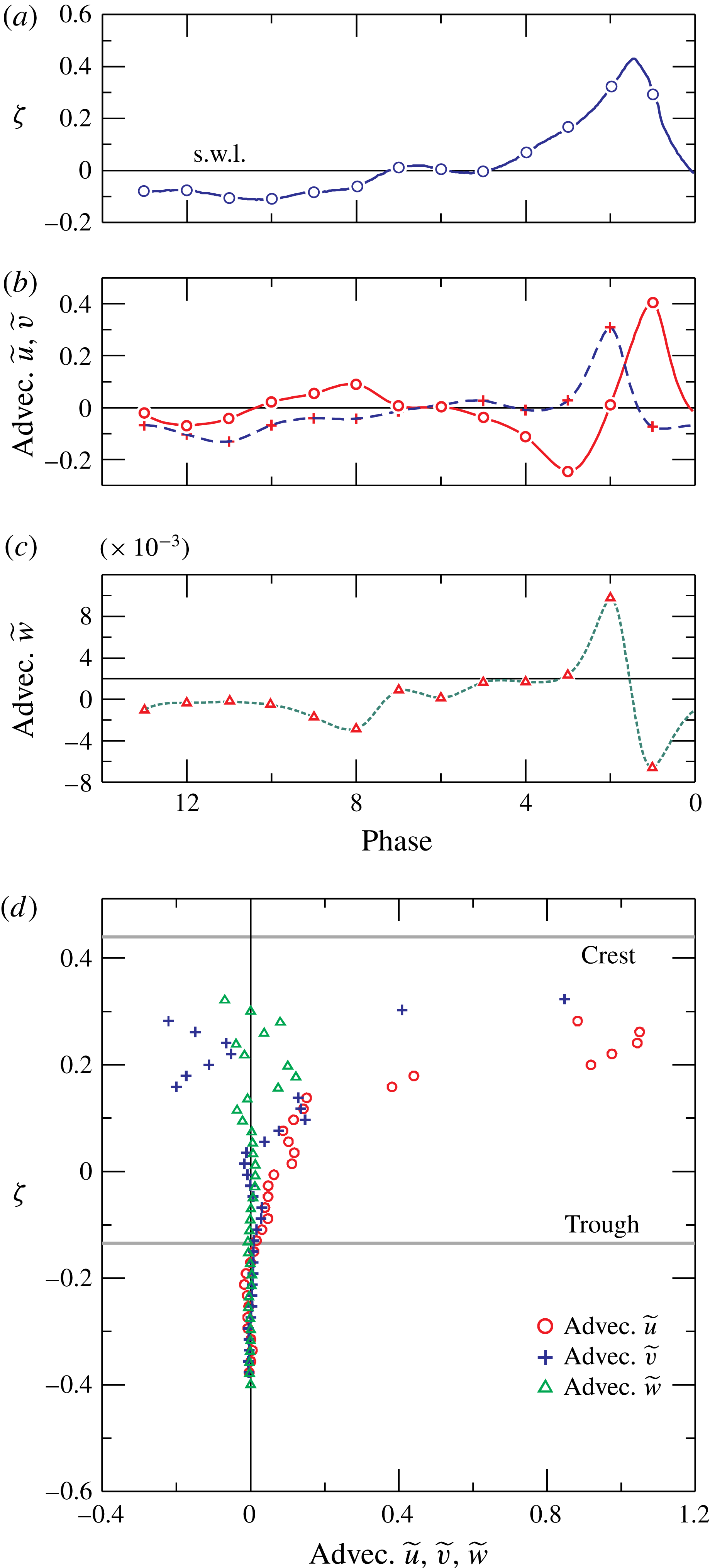
Figure 10 shows the same data as shown in figure 9, but integrated in the vertical direction. The net fluxes during a wave period in the three directions are slightly unbalanced, as a consequence of the missing data below or above the vertical limits of the FOV and the overall uncertainty of the measurements. However, the results are quantitatively coherent with other similar experiments. Figure 10(d) also depicts the time-averaged cross-shore velocity (the undertow). This profile is shown for all the experiments in figure 25 in the Appendix. Figure 11 shows the advection terms due to the mean flow. The cross-shore and the vertical advection are of the same order of magnitude, and the alongshore advection is of a lower order. During breaking, the cross-shore advection is mainly positive, whilst the vertical advection is negative (see figure 11 b) and shows a phase lag of approximately $\unicode[STIX]{x03C0}/2$ (it is not exactly equal to $\unicode[STIX]{x03C0}/2$ , see the following analysis). In the post-breaking phases, a flow reversal is observed in the sign changes for both components. The correlation between the oscillating velocity components, also called the wave Reynolds stress or $\overline{\widetilde{u}\widetilde{v}}$ (shear stress in the $x{-}y$ plane; the other terms are of minor relevance and are not shown) is depicted in figure 12 for all the experiments. The presence of a correlation between the oscillating components is not predicted by the linear theory, and is responsible for current driving (see, e.g. Deigaard & Fredsøe Reference Deigaard and Fredsøe1989). Figure 12(a,c) show the values averaged in the vertical for each phase. The values are generally positive, and the largest values occur during breaking, and are negative immediately after breaking. (b,d) Show the vertical distribution of the cycle-averaged values. The (phasic cycle average) correlation is positive beneath the trough and is increasing in the vertical for experiments 1b–5b ( $T=1.5~\text{s}$ ) and decreasing in the vertical for experiments 6b–9b ( $T=2.0~\text{s}$ ). The linear variation in $\overline{\widetilde{u}\widetilde{v}}$ agrees with several models developed for dissipative or non-dissipative waves, on horizontal or inclined bottoms, and with or without vorticity (see Deigaard & Fredsøe Reference Deigaard and Fredsøe1989; Rivero & Arcilla Reference Rivero and Arcilla1995). However, there are inconsistent results for the trend and sign of the wave Reynolds stress. A very recent analysis (Olfateh et al. Reference Olfateh, Ware, Callaghan, Nielsen and Baldock2016) of the inconsistent results obtained in labs for the wave Reynolds stress (mainly in wind-generated waves, with transfer of momentum and energy from the wind to the waves) demonstrates that the inconsistencies are due to the reflection of the waves. Hence, there is a lab distortion in the experimental results that should always be considered in the data analysis, but the effect should also be present in nature, where multiple sources of wave reflections can be observed (Baquerizo et al. Reference Baquerizo, Losada, Smith and Kobayashi1997).

Figure 10.

Experiment 9b. (a) Phase-averaged surface elevation; (b) vertical integrated phase-averaged horizontal (continuous line) and vertical (dashed line) velocity; (c) vertical integrated phase-averaged alongshore velocity; (d) cycle integrated velocity components (symbols) and time-average horizontal velocity (solid red line).

Figure 11.

Experiment 9b. (a) Phase-averaged surface elevation; (b) vertical integrated advection for the phase-averaged horizontal (solid line) and vertical (dashed line) velocity; (c) vertical integrated advection for the phase-averaged alongshore velocity; (d) cycle integrated advection of the three velocity components.

Figure 12.

Correlation $\widetilde{u}\widetilde{v}$ for all experiments: (a) vertical average values at different phases for experiments 1b–5b; (b) wave cycle phasic-average values, distribution in the vertical; (c,d) similar data as presented in (a,b) but for experiments 6b–9b.

Figure 13 shows four directly estimated terms of the six terms in the linear momentum balance equation in the cross-shore direction. Local inertia (a) is generally dominant, with advection (b) of a smaller order of magnitude, except immediately after breaking (phase 2). Additionally, the turbulent (Reynolds) stress contribution (c) becomes relevant essentially during breaking (phase 1 and 2), whereas the viscous stress contribution (d) is three orders of magnitude smaller than all other contributions. Figure 13(e) shows the net gradient pressure term (excluding the hydrostatic component), computed by summing all the estimated terms. In the overall balance, we note that the turbulent stresses are quite significant immediately after breaking (in phase 2, they are approximately 10 % of the local inertia), act like inertia and require an extra gradient pressure.

Figure 13.

Experiment 9b. Balance for the cross-shore momentum, phase-averaged values. (a) Local inertia (term $I_{m}$ in (4.2)); (b) advection (term $II_{m}$ ); (c) contribution of turbulent (Reynolds) stresses (term $VI_{m}$ ); (d) contribution of viscous stresses (term $V_{m}$ ); (e) net gradient pressure term, equal to $III_{m}+IV_{m}$ , estimated by summing up all the other terms. The second horizontal axis indicates the values as a fraction of gravity.

Figure 14.

Experiment 9b. (a) Phase-averaged surface elevation with the indication of the phase; (b) terms in linear momentum balance in the cross-shore direction, (c) in the vertical direction, and (d) in the alongshore direction. The dashed line refers to local inertia (term $I_{m}$ ), the dotted line refers to advection (term $II_{m}$ ), the dashed-dotted line refers to turbulent stress contribution (term $VI_{m}$ ), and the solid line indicates the net gradient pressure (pressure excluding the hydrostatic component, which is absent in the alongshore direction) obtained by summing up all the other terms. The triangles represent the viscous term contribution (term $V_{m}$ ) which is almost negligible in all the three directions.

The phase-resolved contributions integrated in the vertical are shown in figure 14 for the cross-shore ( $x$ ), the vertical ( $y$ ) and the alongshore ( $z$ ) directions. In the cross-shore direction (b), for most of the wave cycle the net gradient pressure balances only local inertia, because advection and the turbulent stress contribution are negligible. Only beneath the crest does the gradient pressure act against local inertia, advection and turbulent stresses, and it is equal to approximately three times the gravity component parallel to the bottom or a quarter of the value of gravity. For plunging breakers, the peak gradient pressure is much stronger, up to 5 g (see, e.g. Peregrine Reference Peregrine1983)). We recall here that the present data are missing the peak values. In the vertical direction (c), advection is comparable to local inertia immediately before breaking, with positive values, and the subsequent phases are almost completely dominated by local inertia. Turbulent stresses play a minor role with respect to the cross-shore dynamics, and viscous stresses are negligible. In the alongshore direction (d), all terms are much smaller than in the other two directions. In the presence of a rigorous symmetry, flat profiles were expected for all the terms, and the presence of a periodic variation in the inertial terms clearly indicates that alongshore dynamics are triggered by instabilities of various origins, including systematic asymmetries in the breaker, which is a 3D phenomenon. It is expected that in larger flumes these 3D effects are more evident. Notably, the inertial terms and turbulent stresses are comparable during the entire wave cycle.

Figure 15.

Net gradient pressure term in the $x$ (cross-shore) and $y$ (vertical) directions, and breaking wave profile for experiments 9b–8b–7b–6b (panels a–d). The solid blue line is the wave profile (referred to the right vertical axis), filled circles (dashed red line, an interpolation of the experimental values with splines) are the estimated net pressure gradient term in the cross-shore direction, empty squares (dotted green line) are the estimated net pressure gradient term in the vertical direction. The net pressure gradient terms are referred to the left vertical axis.

The gradient pressure term is considered a key element in the shape of the profile of the breaker. It achieves the highest values during steepening of the wave crest, and strongly contributes to the aspect of the breakers and to the post-breaking wave profile evolution. Figure 15(a–d) shows the net pressure gradient terms in the $x$ and $y$ directions for the $T=2.0~\text{s}$ wave tests. The net pressure gradient term in both directions oscillates, following the wave profile but with a phase shift (a steep front, see (a) and (b) is forced by the large positive value of the cross-shore pressure gradient, with a peak value delayed with respect to the wave crest; the delay is reduced for smaller wave breaking height, see (c) and (d), being zero several times and the cross-shore one being the largest in most cases, but not as large as would be expected. Steepening of the wavefront is strongly correlated with the cross-shore net pressure gradient term, while smoothing of the wave profile is correlated with the vertical component of the net pressure gradient. The results for the other waves (with period $T=1.5~\text{s}$ ) are similar (not shown).

Figure 16.

Experiment 9b, Reynolds stress tensor. Phase-averaged normal stress in the (a) $x$ direction, (b) $y$ direction, and (c) $z$ direction. Shear stresses in the (d) $x{-}y$ plane, (e) $x{-}z$ plane, and (f) $y{-}z$ plane.

Figure 16 shows the six phase-averaged components (phasic values) of the Reynolds stress tensor for experiment 9b. The main diagonal term of the tensor is the cross-shore direction term ( $\widetilde{u^{\prime }u^{\prime }}$ , (a)), with two maxima in the crest immediately before and after breaking (phases 1 and 2, respectively). The first maximum is the highest in most of the vertical column of water. Then, a progressive reduction is observed, with a minimum value during the trough phase. The profiles are non-monotonic, and the values decrease beneath the surface elevation, reaching a minimum at $\unicode[STIX]{x1D701}\approx -0.35$ , then increasing again. The bottom of the flume is too far away to be responsible, and this behaviour can be attributed to a memory effect of the previous breaker. The turbulent stresses decay due to dissipation, but are still present when a new breaker arrives. These data also include the effects of the alongshore aligned large eddies moving offshore (Li & Dalrymple Reference Li and Dalrymple1998). The diagonal term $\widetilde{v^{\prime }v^{\prime }}$ in the vertical direction (b) and $\widetilde{w^{\prime }w^{\prime }}$ in the alongshore direction (c) are similar to $\widetilde{u^{\prime }u^{\prime }}$ , even though they both exhibit maximum values in the crest immediately after breaking in phase 2. The term $\widetilde{w^{\prime }w^{\prime }}$ is also much smaller than the other two terms, with a ratio of $\widetilde{w^{\prime }w^{\prime }}/\widetilde{u^{\prime }u^{\prime }}\approx 0.22$ , whereas $\widetilde{v^{\prime }v^{\prime }}/\widetilde{u^{\prime }u^{\prime }}\approx 0.55$ . These values are different for different phases, and vary in the ranges of $0.1<\widetilde{w^{\prime }w^{\prime }}/\widetilde{u^{\prime }u^{\prime }}<0.36$ and $0.36<\widetilde{v^{\prime }v^{\prime }}/\widetilde{u^{\prime }u^{\prime }}<0.86$ . Table 2 reports some values of the TKE distribution (defined as $1/2(u^{\prime }u^{\prime }+v^{\prime }v^{\prime }+w^{\prime }w^{\prime })$ ) for different flow fields. In addition, De Serio & Mossa (Reference De Serio and Mossa2006) found $0<\widetilde{v^{\prime }v^{\prime }}/\widetilde{u^{\prime }u^{\prime }}<0.3$ and $0.1<\widetilde{v^{\prime }v^{\prime }}/\widetilde{u^{\prime }u^{\prime }}<0.5$ for spilling and plunging waves, respectively, with the range indicating the variation in the vertical and the minimum values near the bottom. The tangential stresses in the $x{-}y$ plane and the $y{-}z$ plane are of almost equal intensity. Figure 17(a,b) depicts the phase-resolved Reynolds stress tensor averaged in the vertical. The maximum TKE level occurs in the breaking phase (a). The shear stress in the $x{-}y$ plane is at the positive maximum during breaking and negative maximum immediately after (b). Also, the shear stress in the $y{-}z$ plane is lowest at the breaking point and is positive in all other phases. This behaviour, again, indicates alongshore dynamics, which in theory should be balanced for symmetry. The residual shear stress in the $x{-}z$ plane is almost negligible. Figure 17(d) shows the components of the Reynolds stress tensor integrated over a cycle and resolved in the vertical direction. The largest values of the (phasic) TKE are between the trough and the crest. Also, the time-averaged values are shown in curves that decay in the crest because the water concentration decreases.

Table 2.

Turbulent kinetic energy distribution. The values by Townsend (Reference Townsend1976) refer to plane wakes and have been commonly assumed in computing the turbulent kinetic energy under breaking waves having measured only the two main components of the velocity, see, for example, Stive & Wind (Reference Stive and Wind1982); the values by Nezu & Nakagawa (Reference Nezu and Nakagawa1993) refer to the intermediate region of an open channel; the values by Longo (Reference Longo2011) are beneath a fluctuating free surface.

Figure 17.

Experiment 9b, Reynolds stress tensor. (a) Phase-averaged surface elevation with the indication of the phases; (b) phase-averaged normal stresses (diagonal terms) and TKE ( $k$ , solid line); (c) phase-averaged shear stresses (non-diagonal terms); (d) cycle-averaged stresses, with filled circles indicating the TKE and the solid black line indicating the time-average (non-phasic) TKE. The dotted, dashed and dashed-dotted lines are the time-average (non-phasic) values of the normal stresses.

5 Turbulent kinetic energy balance

The governing equation for the average turbulent kinetic energy can be written as (e.g. Tennekes & Lumley Reference Tennekes and Lumley1972):

where $k=1/2(u_{i}^{\prime }u_{i}^{\prime })$ is the instantaneous turbulent kinetic energy, $\unicode[STIX]{x1D708}$ is the kinematic viscosity, $\widetilde{\unicode[STIX]{x1D61A}_{ij}}=1/2(\widetilde{u_{i,j}}+\widetilde{u_{j,i}})$ is the average rate of strain and $\unicode[STIX]{x1D61A}_{ij}^{\prime }=1/2(u_{i,j}^{\prime }+u_{j,i}^{\prime })$ is the fluctuating rate of strain. The terms are conventionally defined as ( $I_{k}$ ) local inertia, ( $II_{k}$ ) advection by mean flow, ( $III_{k}$ ) transport due to gradient pressure, ( $IV_{k}$ ) transport by velocity fluctuations, ( $V_{k}$ ) transport by viscous stresses, ( $VI_{k}$ ) production, and ( $VII_{k}$ ) viscous dissipation. The transport terms redistribute turbulent kinetic energy; the production term normally represents a transfer of energy from the mean flow to the fluctuating components; and the dissipation is defined as positive, and is a sink of energy for the turbulent flow, with transfer into heat. Figure 18 shows the phase-resolved averages for most of the terms in (5.1) for experiment 9b. The local inertia of TKE (figure 18 a) is mainly negative in the post-breaking phase, and it is generally smaller than the other contributions (except for the dissipation term) and assumes the largest (absolute) values in the phases immediately after breaking. Advection (see figure 18 b) is generally positive and directed onshore (because the alongshore and vertical contributions are minimal). Advection is quite effective in transferring TKE from the generation zone towards the swash zone. Its maximum value is immediately after breaking at the crest. Amongst the transport terms, the only one that can be directly estimated is the transport due to turbulence itself (term $IV_{k}$ , figure 18 c) (additionally, the transport term due to viscosity, term $V_{k}$ , can be estimated, but it is negligible). The transport due to turbulence is generally positive and partly counteracts the advection. A minor role is played by dissipation (figure 18 e) and by the production term (figure 18 d), which in some phases is negative. The production term is positive in most flows, but there is no restriction to its sign and it has been found be negative (i.e. a transfer of energy from turbulence to the mean flow) in experiments (e.g. Beguier et al. Reference Beguier, Giralt, Fulachier, Keffer and Fiedler1978; Liberzon et al. Reference Liberzon, Lthi, Guala, Kinzelbach and Tsinober2005) and in numerical simulations (e.g. Gayen & Sarkar Reference Gayen and Sarkar2011). Figure 18(f) depicts the transport term $III_{k}$ due to pressure fluctuations, which has been estimated by balancing all the other terms in (5.1).

Figure 18.

Experiment 9b, TKE balance equation, phase-averaged values. (a) Local inertia ( $I_{k}$ ); (b) advection by mean flow ( $II_{k}$ ); (c) transport by velocity fluctuations ( $IV_{k}$ ); (d) production ( $VI_{k}$ ); (e) dissipation ( $VII_{k}$ ); (f) estimated transport due to gradient pressure ( $III_{k}$ ). Transport by viscous stresses is negligible.

Figure 19.

Experiment 9b, TKE balance equation, values averaged in the vertical. (a) Surface elevation with the indication of the phases; (b) local inertia, advection by the mean flow and transport by velocity fluctuations; (c) production and dissipation terms, with the solid red line representing the estimated transport due to gradient pressure; (d) time–phasic-averaged terms. The solid line represents the estimated transport due to gradient pressure. Transport by viscous stresses is negligible.

Figure 20.

Ratio between the dissipation rate for isotropic turbulence and dissipation rate for the non-isotropic turbulence. (a) Phase-resolved ratio averaged in the vertical and (b) ratio averaged in the vertical for experiments 1b–5b, with $T=1.5~\text{s}$ . The bars indicates one standard deviation (STD) of the 10 cycles sample drawn for experiment 2b; (b) phase-resolved ratio averaged in the vertical for experiments 1b–5b, with $T=1.5~\text{s}$ ; (c,d) as for (a,b) for experiments 6b–9b, with $T=2.0~\text{s}$ . The bars indicates one STD of the 10 cycles sample drawn for experiment 6b. The hatched area in (a) and in (c) indicates the phase of breaking, which is slightly different for our set of experiments.

Figure 21.

Comparison of spatial gradient of TKE computed with the ‘frozen turbulence’ hypothesis with $\widetilde{u}$ and $C$ as velocity of advection. Results for experiment 5b: (a) all phases and (b) integrated in the vertical. Results for experiment 9b: (c) all phases and (d) integrated in the vertical. The vertical lines in the panels (a and c) indicate the breaking phase.

Figure 19(a–c) shows the same data as shown in figure 18, but integrated in the vertical direction. Advection, transport and production provide the most relevant contribution across the breaking phase, with negligible values for the intrinsic variation in $k$ and the dissipation. The estimated transport due to the pressure gradient term ( $III_{k}$ ) changes sign across the breaking process, and counteracts transport due to fluctuating velocity components (term $IV_{k}$ ). Figure 19(d) shows the data integrated over a wave cycle in phasic values. Again, advection, transport and production dominate the balance below the crest, whereas production changes sign; it is positive in the crest and negative for $\unicode[STIX]{x1D701}<\approx 0.15$ . One of the terms often approximated in modelling TKE is the dissipation rate. The numerous terms necessary to estimate the dissipation rate are seldom available in experimental data sets (direct numerical simulations perform much better in providing virtually all the terms, even though at high Reynolds number some models are adopted for the integration of the equations). Hence, in most cases, the hypothesis of isotropic turbulence is made, with an estimation of the dissipation rate given by (e.g. Tennekes & Lumley Reference Tennekes and Lumley1972)

The present experimental data set allows the estimation of the dissipation rate $\unicode[STIX]{x1D716}$ according to its definition in (5.1) (term $VII_{k}$ ), and a comparison of the ratio $\unicode[STIX]{x1D716}_{isot}/\unicode[STIX]{x1D716}$ , shown in figure 20 for all the experiments, with integration in the vertical (panels a and c) and for the wave cycle (panels b and d). In most of the present experiments results $\unicode[STIX]{x1D716}_{isot}>\unicode[STIX]{x1D716}$ . However, we bear in mind that the limited spatial resolution (0.4 cm grid step) and the limited temporal resolution (7.25 Hz) of the present experimental data do not allow an accurate estimation of dissipation, which typically occurs at very small scales. Hence, the observed values in the present experiments are presumably underestimated, either computed including all the terms or by assuming the isotropic state. For this reason, the terms obtained as closure of the balance should be taken as an approximation.

In the analysis of experimental data based on measurements at a single point (e.g. LDV measurements), the spatial gradients are unknown, and only time gradients can be computed. The spatial gradient terms are computed, whenever necessary, using the hypothesis of ‘frozen turbulence’. Essentially, it is assumed that turbulence (as well as other ‘scalars’ of the flow field) moves like a permanent wave satisfying the condition $\text{d}\widetilde{k}/\text{d}t=0$ , where $\text{d}/\text{d}t$ the total derivative. Hence, it is possible to map the spatial gradients using the time gradient with the transformation $\unicode[STIX]{x2202}/\unicode[STIX]{x2202}t+u\unicode[STIX]{x2202}/\unicode[STIX]{x2202}x=0$ , where $u$ an advective velocity. The advective velocity can be the phase-averaged cross-shore velocity or the celerity of the waves. Figure 21 shows a comparison between the experimental value of the local inertia of TKE and its estimation based on frozen turbulence with advection based on the phase-averaged cross-shore velocity and on the phase celerity of the wave, for experiment 5b ( $T=1.5~\text{s}$ ) and experiment 9b ( $T=2.0~\text{s}$ ). While the estimation based on the phase-averaged cross-shore velocity is acceptable in most phases (discrepancies are relevant in the breaking phases), the estimation based on the phase celerity is biased by significant over- or underestimates. Similar results are obtained for the other variables (not shown).