1 Introduction
Many previous studies have focused on the flow around a circular cylinder in an unbounded flow. In the Stokes range (
 $Re=Ud/\unicode[STIX]{x1D708}\ll 1$
), viscous effects dominate the flow. The flow around a stationary cylinder remains attached and symmetrical about the spanwise and streamwise axes through the centre point of the cylinder. As the Reynolds number is increased, the flow loses its upstream/downstream symmetry as the fluid separates at the rear of the cylinder. This results in the formation of two closed recirculation zones, first occurring at
 $5\lesssim Re\lesssim 7$
(Taneda Reference Taneda1956; Dennis & Chang Reference Dennis and Chang1970). The length of these recirculation regions was found to increase linearly with
 $Re$
, until at
 $Re\simeq 46$
, the wake becomes absolutely unstable and undergoes a transition to a periodic flow state (Roshko Reference Roshko1954; Taneda Reference Taneda1956; Provansal, Mathis & Boyer Reference Provansal, Mathis and Boyer1987; Henderson Reference Henderson1997). This transition is the result of a Hopf bifurcation (i.e. a steady to unsteady transition) of the steady flow that occurs as the flow becomes globally absolutely unstable (Provansal et al.
Reference Provansal, Mathis and Boyer1987; Henderson Reference Henderson1997). The saturated state of vortex shedding in the wake of the cylinder takes the form of a Bénard–von Kármán vortex street (Bénard Reference Bénard1908; von Kármán Reference von Kármán1911) that is characterised by a periodic, repeating pattern of swirling vortices of opposite sign that are shed from the rolled-up shear layers.
As the Reynolds number is increased further, the now-periodic wake undergoes a further transition to three-dimensional flow. Williamson (Reference Williamson1988) found that two clearly identifiable transitions take place sequentially that are distinguished by the development of distinct spatio-temporal three-dimensional wake states designated Mode
 $A$
and Mode
 $B$
. The first of these transitions is also accompanied by a discontinuity in the Strouhal–Reynolds number curve. The Mode
 $A$
instability appears beyond
 $Re\approx 190$
(Williamson Reference Williamson1996b
; Henderson Reference Henderson1997), resulting in pairs of counter-rotating streamwise vortices forming along the span of the cylinder. This three-dimensional mode has a spanwise wavelength of
 $\unicode[STIX]{x1D706}\approx 4d$
, where
 $d$
is the diameter of the cylinder. The second transition to Mode
 $B$
becomes fully developed at
 $Re=260$
and has a preferred spanwise wavelength of
 $\unicode[STIX]{x1D706}\simeq 0.8d$
(Williamson Reference Williamson1996b
; Henderson Reference Henderson1997). The remnants of the streamwise Mode
 $B$
vortical structures can be seen at much higher Reynolds numbers, well beyond the development of fully turbulent flow (e.g. Wu et al.
Reference Wu, Sheridan, Welsh and Hourigan1996).
Imposing a rotation on a cylinder in an unbounded flow has a strong influence on the wake structure and transitions. The degree of rotation is often quantified by the non-dimensional rotation rate,
 $\unicode[STIX]{x1D6FC}=\unicode[STIX]{x1D714}d/(2U)$
, defined as the ratio of the tangential surface speed (
 $\unicode[STIX]{x1D714}d/2$
, with
 $\unicode[STIX]{x1D714}$
the angular velocity) and the free-stream speed
 $U$
. Many authors, including Tang & Ingham (Reference Tang and Ingham1991), have shown that imposing a rotation on the body renders the wake asymmetrical and, at
 $Re\leqslant 60$
, depending on the rotation rate, the elimination of one or both of the recirculation regions in the wake can be observed. For larger
 $Re$
, the imposed rotation may also suppress or delay the transition to unsteady flow in comparison to the case of a non-rotating body.
For the non-rotating cylinder, as the Reynolds number is increased, the wake becomes unsteady. At low rotation rates, a Bénard–von Kármán vortex street is observed (Jaminet & Atta Reference Jaminet and Atta1969), also known as Mode I shedding. For higher values of
 $\unicode[STIX]{x1D6FC}$
, the unsteady wake narrows and is displaced in the direction of motion of the cylinder surface (Díaz et al.
Reference Díaz, Gavaldà, Kawall, Keffer and Giralt1983; Mittal & Kumar Reference Mittal and Kumar2003). As the rotation rate increases beyond a critical value of
 $\unicode[STIX]{x1D6FC}_{c}\simeq 2$
(Díaz et al.
Reference Díaz, Gavaldà, Kawall, Keffer and Giralt1983; Mittal & Kumar Reference Mittal and Kumar2003), the unsteady flow is completely suppressed. Instead of vortex shedding, the surrounding fluid is entrained by the rotation of the body and creates a layer around the cylinder that thickens as
 $\unicode[STIX]{x1D6FC}$
increases (Díaz et al.
Reference Díaz, Gavaldà, Kawall, Keffer and Giralt1983; Mittal Reference Mittal2000). Perhaps surprisingly, a second shedding regime is observed over a specific range of
 $\unicode[STIX]{x1D6FC}$
at much higher
 $\unicode[STIX]{x1D6FC}$
(Mittal & Kumar Reference Mittal and Kumar2003; Kumar, Cantu & Gonzalez Reference Kumar, Cantu and Gonzalez2011), where single-sided vortex shedding occurs with a period much longer than that of Mode I shedding. This wake state is referred to as Mode II shedding.
Limited investigations have been carried out on the development of three-dimensional wakes for a rotating cylinder. At low rotation rates,
 $\unicode[STIX]{x1D6FC}<1$
, Akoury et al. (Reference Akoury, Braza, Perrin, Harran and Hoarau2008) found that Mode
 $A$
becomes unstable at higher Reynolds numbers as
 $\unicode[STIX]{x1D6FC}$
is increased. At higher rotation rates, the flow becomes increasingly unstable to perturbations at
 $Re=200$
in the range
 $3\leqslant \unicode[STIX]{x1D6FC}\leqslant 5$
(Meena et al.
Reference Meena, Sidharth, Khan, Mittal, Mittal and Biswas2011). Recent numerical and experimental investigations (Mittal & Kumar Reference Mittal and Kumar2003; Radi et al.
Reference Radi, Thompson, Rao, Hourigan and Sheridan2013; Rao et al.
Reference Rao, Leontini, Thompson and Hourigan2013a
,Reference Rao, Leontini, Thompson and Hourigan
b
) have identified several new three-dimensional transitions for
 $Re<400$
. In the Mode I shedding regime, five three-dimensional modes were found to become unstable and, in the steady regime of flow
 $\unicode[STIX]{x1D6FC}\gtrsim 2$
, four three-dimensional modes were observed.
When the presence of a wall is considered, Taneda (Reference Taneda1965) showed that a stationary wall near a cylinder stabilises the flow. Arnal, Goering & Humphrey (Reference Arnal, Goering and Humphrey1991) found that the onset of unsteady flow in the presence of a wall is shifted to
 $Re\approx 100$
, from
 $Re\approx 46$
for an isolated cylinder in a free stream. This finding is correct as long as the gap ratio between the cylinder and the wall does not exceed a certain critical value, which depends on the Reynolds number. The steady flow around a stationary cylinder on a wall is similar to that of a backward-facing step (Armaly et al.
Reference Armaly, Durst, Pereira and Schönung1983); it is characterised by a single recirculation region, surrounded by fluid which separates from the body and reattaches on the wall downstream. However, the behaviour of the flow depends on many parameters: the distance between the cylinder and the wall, the motion of the wall relative to the cylinder and the imposed rotation of the body.
Stewart et al. (Reference Stewart, Thompson, Leweke and Hourigan2010) investigated the case of a rotating cylinder translating next to a moving wall at rotation rates in the range
 $-1<\unicode[STIX]{x1D6FC}<1$
. In the steady flow regime, two recirculation zones are observed in the wake, and the drag and lift forces decrease as
 $Re$
increases. Prograde rolling (
 $\unicode[STIX]{x1D6FC}>0$
) was found to destabilise the flow whereas retrograde rotation (
 $\unicode[STIX]{x1D6FC}<0$
) delayed the onset of unsteady flow. This was later confirmed/extended in a study by Rao et al. (Reference Rao, Stewart, Thompson, Leweke and Hourigan2011) for which higher values of
 $\unicode[STIX]{x1D6FC}$
were considered.
For unsteady flows in the wake of a cylinder placed near a wall, the strength of the vortex shedding decreases as the cylinder is placed closer to the wall (Lei, Cheng & Kavanagh Reference Lei, Cheng and Kavanagh1999). At
 $Re=170$
, Taneda (Reference Taneda1965) observed a single row of vortices for a cylinder moving near a wall. In the unsteady regime, vortex pairs with a net rotation appear in the wake as a result of the interaction between the shear layer shed from the top of the cylinder and induced secondary shedding from the wall boundary layer vorticity downstream (Stewart et al.
Reference Stewart, Thompson, Leweke and Hourigan2010; Rao et al.
Reference Rao, Stewart, Thompson, Leweke and Hourigan2011). Unlike the case of a cylinder placed in a free stream but similar to the flow over a backward-facing step, the wake undergoes a transition to three-dimensionality before the onset to two-dimensional vortex shedding (Stewart et al.
Reference Stewart, Thompson, Leweke and Hourigan2010; Rao et al.
Reference Rao, Stewart, Thompson, Leweke and Hourigan2011).
In the current study, the results of Stewart et al. (Reference Stewart, Thompson, Leweke and Hourigan2010) for a cylinder rolling at
 $\unicode[STIX]{x1D6FC}=1$
without slipping on a wall are extended to identify and characterise the different saturated flow states and modes of the three-dimensional instability, and their influence on the underlying two-dimensional structure of the flow. A more detailed description of the problem, the corresponding equations and the numerical methods are given in the first section of this paper. Then follow the results from the linear stability analysis and Floquet analysis, highlighting the appearance of new modes of the three-dimensional instability. Thorough comparisons of the similarities and differences in the flow structures and fluid forces show how the two-dimensional simulations can be used confidently to approximate this problem during the initial stage of flow development. The essential findings of this work are then summarised in the last section, along with some discussion of future research extending from this paper.
2 Problem description and methodology
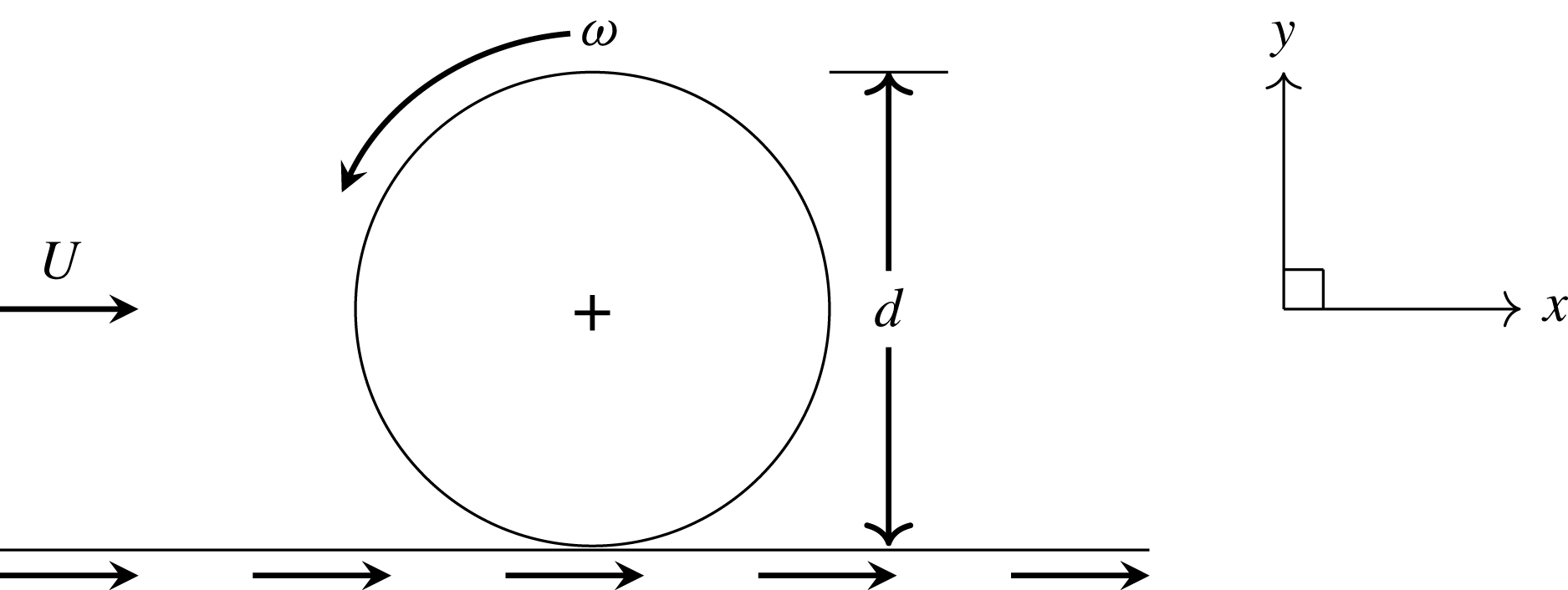
A two-dimensional schematic of the problem under consideration: a cylinder of diameter
 $d$
is rolling along a wall. The translational and angular velocities are represented by
 $U$
and
 $\unicode[STIX]{x1D714}$
, respectively. In the simulations, the inertial frame of reference
 $(x,y)$
is attached to the centre of the body.

Figure 1 illustrates the problem set-up and parameter definitions: a cylinder of diameter
 $d$
is rolling along a wall at a rotation rate
 $\unicode[STIX]{x1D714}$
. For computational simplicity, the frame of reference is placed at the centre of the cylinder, this being equivalent to the fluid and wall moving past the fixed, rotating cylinder at a speed
 $U$
.
2.1 Background to new stability analysis studies
Consider a stationary cylinder placed in a free stream. In the steady, laminar regime below the critical Reynolds number
 $Re_{c,2D}=46$
at which transition to periodic shedding begins, it is well known that two mirror-symmetrical recirculation regions form in the wake whose length increases with the Reynolds number. For Reynolds numbers above the critical value, the steady wake is unstable, causing a decrease in the mean formation length of the recirculation region of the time-averaged flow (Williamson Reference Williamson1996a
,Reference Williamson
b
). Experiments and numerical simulations show that, for a given Reynolds number after the background flow is impulsively started, the evolution of the recirculation region is characterised by a linear, steady increase of its length followed by slowly growing waviness, and eventually, a fully developed Bénard–von Kármán vortex street. Thus in this case, the growth of perturbations leading to a fully developed periodic wake occurs after the steady symmetric wake state has fully (or almost fully) formed (e.g. see Thompson & Le Gal Reference Thompson and Le Gal2004). Moreover, the two-dimensional steady wake is not unstable to three-dimensional perturbations; the first three-dimensional transition occurs on the two-dimensional periodic wake (Williamson Reference Williamson1988).
Conversely, when the cylinder is uniformly rolling along a wall, two-dimensional numerical simulations indicate that well below the critical Reynolds number for sustained two-dimensional (2-D) vortex shedding (
 $Re_{c,2D}=88$
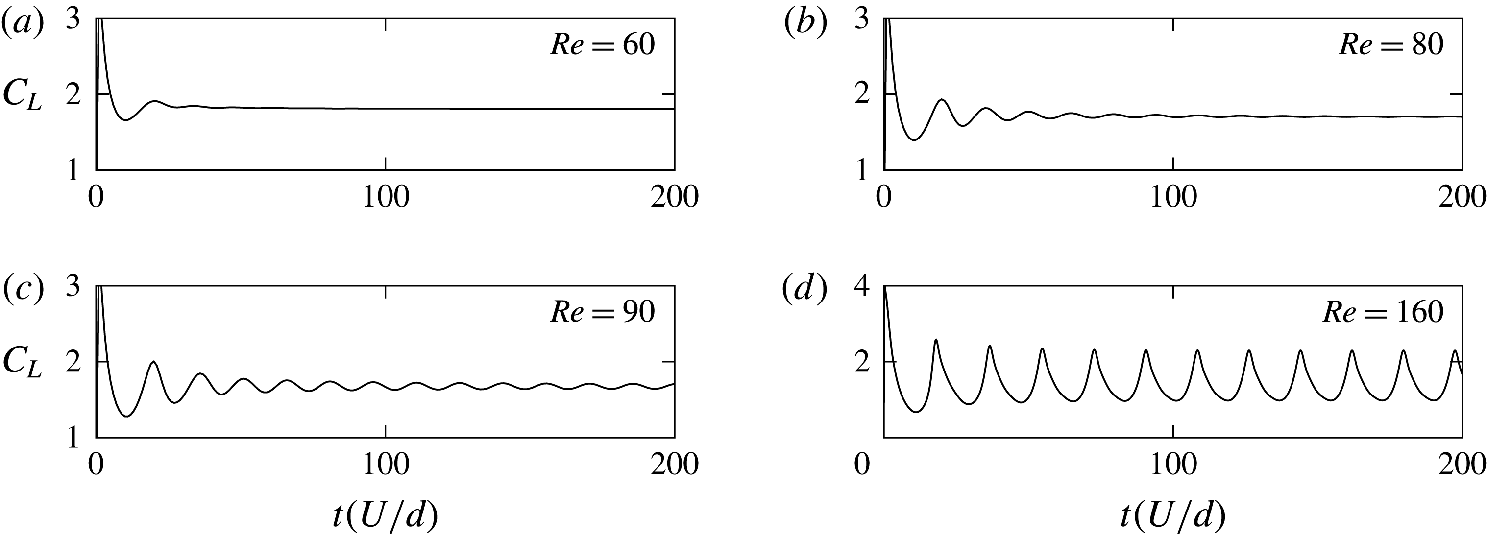
), vortex shedding still occurs almost from startup. This can be seen from figure 2, which shows the time evolution of the lift coefficient for
 $Re=90$
and 160, above the critical Reynolds number. The oscillations in the curves, observed from the initial starting time
 $t_{0}=0$
, are the result of the immediate shedding of vortices into the wake. For
 $Re=90$
, it takes approximately six shedding cycles to reach the asymptotic periodic state, whilst for
 $Re=160$
, well beyond the critical Reynolds number, the transition to the fully developed 2-D periodic state is essentially complete after just two shedding periods. Interestingly, even when the flow is laminar below
 $Re_{c,2D}$
, it undergoes immediate vortex shedding in the first instances of the flow development before settling down to its steady state. This effect was also made visible by Le Gal & Croquette (Reference Le Gal and Croquette2000) who studied experimentally the impulse response of the subcritical wake of a cylinder. These preliminary oscillations are visible on the plots of the lift force on figure 2 for
 $Re=60$
and
 $80$
.
Thus, while Stewart et al. (Reference Stewart, Thompson, Leweke and Hourigan2010) documented that the onset of 3-D flow occurs at a Reynolds number of approximately 40 on a steady recirculating base flow, the actual flow transitions and dynamics observed in practice, for a cylinder rolling along a surface at constant velocity from an impulsive start, may be different. In particular, above the critical Reynolds number for 2-D vortex shedding, a 2-D periodic wake seems likely to essentially fully develop prior to any observable development of three-dimensionality. This hypothesis will be tested in the following sections. It has several consequences. It suggests that 2-D simulations have validity well beyond the critical Reynolds number at which three-dimensionality first occurs for the steady wake, at least for a non-negligible period after impulsive startup. It also suggests that the previously documented 3-D stability analysis (Stewart et al.
Reference Stewart, Thompson, Leweke and Hourigan2010) based on a steady 2-D base flow may not have a strong relevance for the overall wake dynamics for Reynolds numbers above
 $Re_{c,2D}$
. Finally, it is not clear what this means for the fully saturated wake state at different Reynolds numbers. Thus, in this paper, the stability analysis is extended to examine the 3-D stability of the 2-D periodic wake state. This is supplemented by direct 3-D simulations to examine the longer-term wake evolution.
Time evolution (scaled by
 $d/U$
) of the lift coefficient from impulsive startup. (a,b) Evolution for Reynolds number below the transition to 2-D shedding. (c,d) Evolution for Reynolds numbers beyond the transition to vortex shedding.

2.2 Governing equations
The governing equations are the continuity and incompressible Navier–Stokes equations for the motion of the fluid. Let
 $\boldsymbol{u}(x,y,z,t)=(u,v,w)$
represent the velocity of the fluid in Cartesian coordinates. In the case of an incompressible flow, the continuity equation is:
 $$\begin{eqnarray}\unicode[STIX]{x1D735}\boldsymbol{\cdot }\boldsymbol{u}=0,\end{eqnarray}$$
and the general form of the incompressible Navier–Stokes equation is:
 $$\begin{eqnarray}\frac{\unicode[STIX]{x2202}\boldsymbol{u}}{\unicode[STIX]{x2202}t}+\boldsymbol{u}\boldsymbol{\cdot }\unicode[STIX]{x1D735}\boldsymbol{u}=-\frac{1}{\unicode[STIX]{x1D70C}}\unicode[STIX]{x1D735}P+\unicode[STIX]{x1D708}\unicode[STIX]{x1D6FB}^{2}\boldsymbol{u},\end{eqnarray}$$
where
 $\unicode[STIX]{x1D70C}$
is the density of the fluid and
 $P$
is the static pressure. The drag and lift coefficients per unit length are defined in the usual way:
 $$\begin{eqnarray}C_{D}=\frac{D}{\frac{1}{2}\unicode[STIX]{x1D70C}U^{2}d}\quad \text{and}\quad C_{L}=\frac{L}{\frac{1}{2}\unicode[STIX]{x1D70C}U^{2}d},\end{eqnarray}$$
where
 $D$
and
 $L$
represent the drag and lift forces, respectively.
2.3 Numerical scheme
The solver is based on a code that has been used extensively for similar problems, so it will only be described briefly here. Overall, the time-dependent incompressible Navier–Stokes equations for the fluid are solved in Cartesian coordinates using a spectral-element approach, in a cross-sectional plane for 2-D simulations or a combined spectral-element/Fourier approach in three dimensions. The spectral-element method is a formulation of a high-order finite-element method that uses high-order Lagrangian interpolants to approximate the solutions of partial-differential equations. It has the advantage of converging much faster than a typical finite-element method, considering that the error decreases exponentially with the order of the approximating polynomial, all the while retaining some of the flexibility for modelling complex geometries that finite-element methods provide. The (nodal) approach adopted is described in detail in Karniadakis & Sherwin (Reference Karniadakis and Sherwin1999). The spatially discretised equations are then integrated forward in time using a three-step time-splitting approach, where the advection, pressure and diffusion terms are treated separately and sequentially (Chorin Reference Chorin1968; Karniadakis, Israeli & Orszag Reference Karniadakis, Israeli and Orszag1991; Thompson et al.
Reference Thompson, Hourigan, Cheung and Leweke2006). The advection step is carried out using the third-order Adams–Bashforth approach. The pressure and viscous substeps are both solved directly using a lower upper (LU) decomposition, which factors the matrices into a lower triangular matrix
 $\unicode[STIX]{x1D647}$
and an upper triangular one
 $\unicode[STIX]{x1D650}$
(Turing Reference Turing1948), invoking the second-order Adams–Moulton (Crank–Nicholson) approximation for the linear viscous step. Whilst higher-order time-stepping methods could be employed, because typically several hundred time steps are required per shedding cycle to guarantee stability of the iterative approach, there is no discernible improvement in accuracy of the overall solution. The solver is explained in more detail by Thompson et al. (Reference Thompson, Hourigan, Cheung and Leweke2006), and has widely been tested, validated and used for studies of flows around bluff bodies such as cylinders (Thompson, Leweke & Williamson Reference Thompson, Leweke and Williamson2001b
; Ryan, Thompson & Hourigan Reference Ryan, Thompson and Hourigan2005; Rao et al.
Reference Rao, Stewart, Thompson, Leweke and Hourigan2011) and spheres (Thompson, Leweke & Provansal Reference Thompson, Leweke and Provansal2001a
; Thompson et al.
Reference Thompson, Hourigan, Cheung and Leweke2006; Rao et al.
Reference Rao, Passaggia, Bolnot, Thompson, Leweke and Hourigan2012). This code has also been modified to determine the linear stability of base flows, as explained in § 2.4 below.
In addition to the time-dependent solver, a steady solver is required to produce the steady base flows for the linear stability analysis. This is a modified version of the spectral-element code based on the penalty formulation (see Zienkiewicz Reference Zienkiewicz1977). This has been validated for a number of similar flow problems (e.g. Thompson & Hourigan Reference Thompson and Hourigan2003; Jones, Hourigan & Thompson Reference Jones, Hourigan and Thompson2015).
2.4 Linear stability analysis
Linear stability analysis was undertaken in order to quantify flow transitions leading to vortex shedding, and to 3-D flow. For a 2-D steady or periodic base flow
 $\boldsymbol{U}$
, the velocity and pressure perturbation fields (
 $\boldsymbol{u}^{\prime }$
,
 $P^{\prime }$
) satisfy the continuity and linearised Navier–Stokes equations:
 $$\begin{eqnarray}\displaystyle & \displaystyle \unicode[STIX]{x1D735}\boldsymbol{\cdot }\boldsymbol{u}^{\prime }=0, & \displaystyle\end{eqnarray}$$
 $$\begin{eqnarray}\displaystyle & \displaystyle \frac{\unicode[STIX]{x2202}\boldsymbol{u}^{\prime }}{\unicode[STIX]{x2202}t}+\boldsymbol{U}\boldsymbol{\cdot }\unicode[STIX]{x1D735}\boldsymbol{u}^{\prime }+\boldsymbol{u}^{\prime }\boldsymbol{\cdot }\unicode[STIX]{x1D735}\boldsymbol{U}=-\frac{1}{\unicode[STIX]{x1D70C}}\unicode[STIX]{x1D735}P^{\prime }+\unicode[STIX]{x1D708}\unicode[STIX]{x1D6FB}^{2}\boldsymbol{u}^{\prime }. & \displaystyle\end{eqnarray}$$
Because the coefficients are independent of
 $z$
, the perturbation fields can be further decomposed, representing the
 $z$
-dependence of variables as the sum of complex terms of a Fourier expansion:
 $$\begin{eqnarray}\displaystyle u^{\prime }(x,y,z,t) & = & \displaystyle \mathop{\sum }_{k}\hat{u} _{k}(x,y,t)\sin (2\unicode[STIX]{x03C0}z/\unicode[STIX]{x1D706}_{k}),\end{eqnarray}$$
 $$\begin{eqnarray}\displaystyle v^{\prime }(x,y,z,t) & = & \displaystyle \mathop{\sum }_{k}\hat{v}_{k}(x,y,t)\sin (2\unicode[STIX]{x03C0}z/\unicode[STIX]{x1D706}_{k}),\end{eqnarray}$$
 $$\begin{eqnarray}\displaystyle w^{\prime }(x,y,z,t) & = & \displaystyle \mathop{\sum }_{k}{\hat{w}}_{k}(x,y,t)\cos (2\unicode[STIX]{x03C0}z/\unicode[STIX]{x1D706}_{k}),\end{eqnarray}$$
 $$\begin{eqnarray}\displaystyle P^{\prime }(x,y,z,t) & = & \displaystyle \mathop{\sum }_{k}\hat{P}_{k}(x,y,t)\sin (2\unicode[STIX]{x03C0}z/\unicode[STIX]{x1D706}_{k}).\end{eqnarray}$$
Using these expansions, equations (2.4) and (2.5) give for each of the Fourier modes:
 $$\begin{eqnarray}\displaystyle & \displaystyle \frac{\unicode[STIX]{x2202}\hat{u} _{k}}{\unicode[STIX]{x2202}t}=-\!\left(\!\hat{u} _{k}\frac{\unicode[STIX]{x2202}U}{\unicode[STIX]{x2202}x}+\hat{v}_{k}\frac{\unicode[STIX]{x2202}U}{\unicode[STIX]{x2202}y}+U\frac{\unicode[STIX]{x2202}\hat{u} _{k}}{\unicode[STIX]{x2202}x}+V\frac{\unicode[STIX]{x2202}\hat{u} _{k}}{\unicode[STIX]{x2202}y}\!\right)-\frac{1}{\unicode[STIX]{x1D70C}}\frac{\unicode[STIX]{x2202}\hat{P}_{k}}{\unicode[STIX]{x2202}x}+\unicode[STIX]{x1D708}\left(\!\frac{\unicode[STIX]{x2202}^{2}\hat{u} _{k}}{\unicode[STIX]{x2202}x^{2}}+\frac{\unicode[STIX]{x2202}^{2}\hat{u} _{k}}{\unicode[STIX]{x2202}y^{2}}-(2\unicode[STIX]{x03C0}/\unicode[STIX]{x1D706}_{k})^{2}\hat{u} _{k}\!\right)\!, & \displaystyle \nonumber\\ \displaystyle & & \displaystyle\end{eqnarray}$$
 $$\begin{eqnarray}\displaystyle & \displaystyle \frac{\unicode[STIX]{x2202}\hat{v}_{k}}{\unicode[STIX]{x2202}t}=-\!\left(\!\hat{u} _{k}\frac{\unicode[STIX]{x2202}V}{\unicode[STIX]{x2202}x}+\hat{v}_{k}\frac{\unicode[STIX]{x2202}V}{\unicode[STIX]{x2202}y}+U\frac{\unicode[STIX]{x2202}\hat{v}_{k}}{\unicode[STIX]{x2202}x}+V\frac{\unicode[STIX]{x2202}\hat{v}_{k}}{\unicode[STIX]{x2202}y}\!\right)-\frac{1}{\unicode[STIX]{x1D70C}}\frac{\unicode[STIX]{x2202}\hat{P}_{k}}{\unicode[STIX]{x2202}y}+\unicode[STIX]{x1D708}\left(\!\frac{\unicode[STIX]{x2202}^{2}\hat{v}_{k}}{\unicode[STIX]{x2202}x^{2}}+\frac{\unicode[STIX]{x2202}^{2}\hat{v}_{k}}{\unicode[STIX]{x2202}y^{2}}-(2\unicode[STIX]{x03C0}/\unicode[STIX]{x1D706}_{k})^{2}\hat{v}_{k}\!\right)\!, & \displaystyle \nonumber\\ \displaystyle & & \displaystyle\end{eqnarray}$$
 $$\begin{eqnarray}\displaystyle & \displaystyle \frac{\unicode[STIX]{x2202}{\hat{w}}_{k}}{\unicode[STIX]{x2202}t}=-\!\left(\!U\frac{\unicode[STIX]{x2202}{\hat{w}}_{k}}{\unicode[STIX]{x2202}x}+V\frac{\unicode[STIX]{x2202}{\hat{w}}_{k}}{\unicode[STIX]{x2202}y}\!\right)-(2\unicode[STIX]{x03C0}/\unicode[STIX]{x1D706}_{k})\frac{1}{\unicode[STIX]{x1D70C}}\hat{P}_{k}+\unicode[STIX]{x1D708}\left(\!\frac{\unicode[STIX]{x2202}^{2}{\hat{w}}_{k}}{\unicode[STIX]{x2202}x^{2}}+\frac{\unicode[STIX]{x2202}^{2}{\hat{w}}_{k}}{\unicode[STIX]{x2202}y^{2}}-(2\unicode[STIX]{x03C0}/\unicode[STIX]{x1D706}_{k})^{2}{\hat{w}}_{k}\!\right)\!, & \displaystyle \nonumber\\ \displaystyle & & \displaystyle\end{eqnarray}$$
 $$\begin{eqnarray}\displaystyle & \displaystyle \frac{\unicode[STIX]{x2202}\hat{u} _{k}}{\unicode[STIX]{x2202}x}+\frac{\unicode[STIX]{x2202}\hat{v}_{k}}{\unicode[STIX]{x2202}y}-(2\unicode[STIX]{x03C0}/\unicode[STIX]{x1D706}_{k}){\hat{w}}_{k}=0. & \displaystyle\end{eqnarray}$$
These perturbation field modes (
 $\hat{u} _{k},\hat{v}_{k},{\hat{w}}_{k},\hat{P}_{k}$
) can be further expressed as a sum of eigenmodes, each with its own growth rate. After choosing a wavelength and integrating these equations from initially random fields for sufficient time, the velocity perturbation fields will be dominated by the eigenmodes with the largest growth rates. Using a Krylov subspace together with Arnoldi decomposition allows a sequence of evolved fields to be decomposed into the dominant eigenmodes together with their corresponding growth rates (e.g. Mamun & Tuckerman Reference Mamun and Tuckerman1995; Barkley & Henderson Reference Barkley and Henderson1996). If
 $\hat{A}$
represents any of the perturbation fields
 $\hat{u} _{k},\hat{v}_{k},{\hat{w}}_{k}$
and
 $\hat{P}_{k}$
, then this method gives
 $\hat{A}(x,y,t+T)=\hat{A}(x,y,t)\exp (\unicode[STIX]{x1D70E}T)$
, if the eigenmode spatial distribution is not a function of time. Here
 $\unicode[STIX]{x1D70E}$
is the growth rate and
 $T$
is the time interval over which the growth of the mode is recorded. It is also possible to get pairs of eigenmodes that have complex conjugate growth rates, providing the possibility of solutions with a periodic component on top of the exponential time variation. These pairs can also be extracted directly from the Arnoldi decomposition together with the complex growth rates
 $\unicode[STIX]{x1D70E}=\unicode[STIX]{x1D70E}_{r}+\text{i}\unicode[STIX]{x1D70E}_{i}$
. For a 3-D transition on a 2-D periodic base flow, the procedure is the same, with the sequence of perturbation fields forming the Krylov subspace taken at full base flow period intervals
 $T$
. In that case, the approach is called Floquet analysis, and the growth of each eigenmode is often expressed as a Floquet multiplier
 $\unicode[STIX]{x1D707}=\exp (\unicode[STIX]{x1D70E}T)$
, i.e. the amplitude of the mode after it has evolved for one period relative to the initial state. Again, it is possible to have pairs of eigenmodes with complex conjugate Floquet multipliers that are resolved through Arnoldi decomposition. For the 3-D analysis, the eigenmodes depend on the selected spanwise wavelength
 $\unicode[STIX]{x1D706}_{k}$
. If
 $|\unicode[STIX]{x1D707}|>1$
(or
 $\unicode[STIX]{x1D70E}_{r}>0$
), then the perturbation field will be amplified over time, while
 $|\unicode[STIX]{x1D707}|<1$
(or equivalently
 $\unicode[STIX]{x1D70E}_{r}<0$
) for all
 $\unicode[STIX]{x1D706}$
implies that any perturbation will decay and, hence, the flow is linearly stable. Transition occurs when
 $|\unicode[STIX]{x1D707}|=1$
or
 $\unicode[STIX]{x1D70E}_{r}=0$
. For the 3-D case, this condition has to be tested for every possible spanwise wavelength. The (eigen)modes that are obtained with Floquet analysis reported in this paper comprise periods equal to that of the periodic 2-D base flow, twice the period (subharmonic modes) and modes with different periods (quasi-periodic modes). The first two cases are characterised by a growth rate
 $\unicode[STIX]{x1D70E}$
that is real. The quasi-periodic modes have a period that is not commensurate with the base flow period and exist in pairs with complex conjugate Floquet multipliers. More details can be found in Elston, Sheridan & Blackburn (Reference Elston, Sheridan and Blackburn2004), Ryan et al. (Reference Ryan, Thompson and Hourigan2005), Leontini, Thompson & Hourigan (Reference Leontini, Thompson and Hourigan2007), Griffith et al. (Reference Griffith, Thompson, Leweke, Hourigan and Anderson2007, Reference Griffith, Leontini, Thompson and Hourigan2011), Stewart (Reference Stewart2008).
2.5 Domain size and resolution studies
For this study, the Reynolds number range is restricted to be
 $Re\leqslant 300$
, covering flow transitions to vortex shedding and to three-dimensionality.
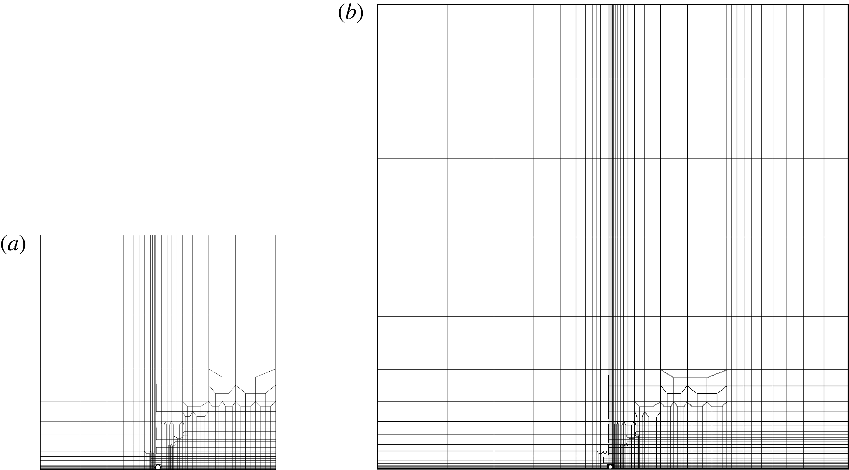
Two domain sizes were investigated to quantify blockage effects. All positions are non-dimensional and are scaled by the diameter of the cylinder. The first mesh
 $M1$
is shown in figure 3 and consists of 1472 macro-elements. The upstream, downstream and upper boundaries are positioned at
 $(x_{1,u},x_{1,d},y_{1})=(-25,25,50)$
, respectively. The second mesh
 $M2$
, also shown on figure 3, consists of 1906 elements and has the dimensions
 $(x_{2,u},x_{2,d},y_{2})=(-50,50,100)$
. Both meshes have increased resolution in the vicinity and downstream of the cylinder that is located at
 $x=0$
and
 $y=0$
. The differences in the drag and lift forces do not exceed 1 % at the highest Reynolds number considered (
 $Re=300$
).
View of the cylinder mesh
 $M1$
:
 $(x_{1,u},x_{1,d},y_{1})=(-25,25,50)$
(a) and
 $M2$
:
 $(x_{2,u},x_{2,d},y_{2})=(-50,50,100)$
(b). The cylinder is placed in the middle of the
 $x$
-axis, and near the wall at a gap ratio of
 $G/d=0.005$
in order to avoid numerical singularities from arising. The flow is from left to right and the resolution in the vicinity and downstream of the cylinder is increased in order to accurately capture the flow structures in the wake.

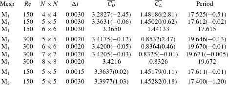
To ensure that the solution is converged with the chosen time step
 $\unicode[STIX]{x0394}t=0.0030$
, the latter was halved to
 $0.0015$
. This produced a variation in the body forces of less than 0.2 % at
 $Re=150$
.
A last resolution study was carried out by increasing the number of the internal node points within each macro-element from
 $N=4\;(\times 4)$
to
 $N=5\;(\times 5)$
,
 $N=6\;(\times 6)$
and
 $N=7\;(\times 7)$
, which is taken as the reference value. We found that the drag force, the lift force and the period of oscillation differ by less than 1 % respectively for
 $N\geqslant 5$
at
 $Re=150$
. At the highest Reynolds number
 $Re=300$
, the drag and Strouhal number are well within the 0.5 % at
 $N=5\;(\times 5)$
whereas the error in the lift force reached 2.5 %. From these results, and, considering that this study focuses mostly on a range of Reynolds number around the transition values
 $Re_{c,3D}$
and
 $Re_{c,2D}$
and up to 160, we can safely conclude that the mesh with 5 nodes per macro-element is converged and use it throughout our simulations.
The point of contact between the cylinder and the wall leads to a mesh singularity, and hence a small gap
 $G$
is imposed between the cylinder and the wall. It has been shown previously that the flow structures visualised in the experiments and those observed numerically are in good agreement with
 $G/d=0.005$
(Stewart et al.
Reference Stewart, Hourigan, Thompson and Leweke2006, Reference Stewart, Thompson, Leweke and Hourigan2010; Rao et al.
Reference Rao, Stewart, Thompson, Leweke and Hourigan2011), while reducing the gap ratio has little effect on flow quantities of interest (Stewart et al.
Reference Stewart, Thompson, Leweke and Hourigan2010) Thus a gap ratio
 $G/d$
of 0.005 was used throughout this investigation.
For the full 3-D nonlinear simulations, a Fourier expansion is used to represent the spanwise dependence of the flow variables (e.g. see Karniadakis & Triantafyllou Reference Karniadakis and Triantafyllou1992; Thompson, Hourigan & Sheridan Reference Thompson, Hourigan and Sheridan1996; Karniadakis & Sherwin Reference Karniadakis and Sherwin1999). The spanwise dimension is set to
 $54d$
for simulations for
 $Re\geqslant Re_{c,2D}$
and
 $25.5d$
for
 $Re<Re_{c,2D}$
. These domains were chosen to fit approximately three wavelengths of the longest-wavelength instability mode predicted by Floquet analysis (
 $\unicode[STIX]{x1D706}\sim 8.5d$
and
 $18d$
for the steady and periodic base states). The choice of such large spanwise domains was to allow nonlinear interactions between all relevant modes as the wake evolves to a fully saturated state. Another option would be to restrict the domain to wavelengths corresponding to each dominant mode to look at the super-/sub-critical nature of the each transition from a linear to a nonlinear state (but not the fully saturated state). This could have been done, but it is not clear it would contribute much to the physical picture. For instance, for the Mode
 $A$
transition of a circular cylinder in free stream, beyond saturation the wake evolves to allow dislocations (e.g. Williamson Reference Williamson1996a
,Reference Williamson
b
) that cannot be represented on a single wavelength spanwise domain. Also relevant, Karniadakis & Triantafyllou (Reference Karniadakis and Triantafyllou1992) used a spanwise width that only allowed Mode
 $B$
to grow. Because of this unphysical restriction, the authors observed period doubling as the route to a fully turbulent flow. However, this does not seem to be the situation for the real wake, or for computations using a sufficiently wide spanwise domain (Henderson Reference Henderson1997). Thus, it was decided to use a wider domain that would not put unphysical restrictions on mode development. Typically 48 and 96 Fourier modes are used for these simulations for the steady and periodic regimes, respectively. Since the shortest-wavelength mode corresponds to
 $\unicode[STIX]{x1D706}\simeq 2.5d$
, this corresponds to approximately 10 Fourier planes to resolve the smallest important scales that develop in the wake. Tests with 144 Fourier modes confirm that this resolution accurately captures the wake evolution for the Reynolds number range considered.
Table 1 reports the results from the different resolution studies mentioned above.
Domain and temporal and spatial resolution study. The numbers in parentheses show the error relative to the highest resolution (or number of nodes
 $N$
) used for the comparison. The mesh M
 $_{1}$
has a blockage ratio of 1 % and the mesh M
 $_{2}$
a blockage ratio of 2 %. Most of the simulations were undertaken with mesh M
 $_{2}$
, noting typical blockage-induced errors in the Strouhal and force coefficients of
 ${\sim}$
2 %. The comparisons indicate that the time-stepping error is negligible, whilst the error induced using
 $5\times 5$
nodes/element is typically
 ${\sim}$
1 % for a Reynolds number of 150.

3 Results
3.1 Linear stability analysis and flow transitions
Experimental studies by Taneda (Reference Taneda1979) showed that the presence of the wall has a stabilising effect on the flow as long as the gap ratio does not exceed a certain critical value (Lei et al.
Reference Lei, Cheng and Kavanagh1999). Stewart et al. (Reference Stewart, Thompson, Leweke and Hourigan2010) investigated the wake behind rolling cylinders at various rotation rates
 $\unicode[STIX]{x1D6FC}$
, and found that as
 $\unicode[STIX]{x1D6FC}$
varies from prograde (
 $\unicode[STIX]{x1D6FC}>0$
) to retrograde (
 $\unicode[STIX]{x1D6FC}<0$
) rolling, the critical Reynolds numbers for three-dimensional (
 $Re_{c,3D}$
) and unsteady (
 $Re_{c,2D}$
) transitions both increase. For comparison with that previous study, these critical Reynolds numbers were again predicted for the reference case of
 $\unicode[STIX]{x1D6FC}=1$
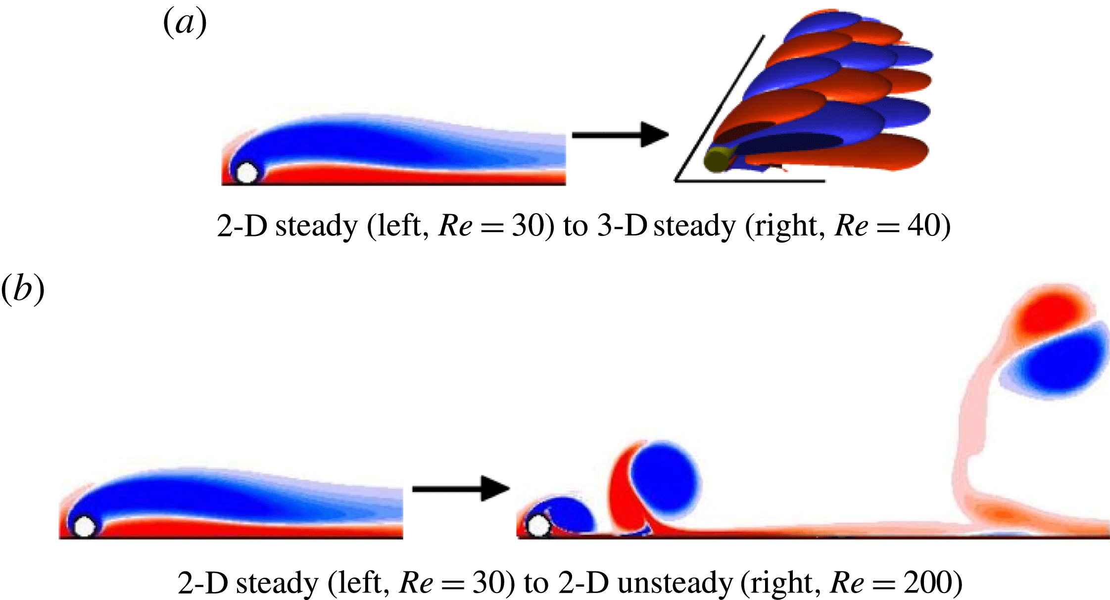
(pure rolling without slipping). These transitions and the resulting flow states are depicted in figure 4.
Visualisation of the initial flow transitions under consideration. The images showing 2-D flow depict the spanwise vorticity field, whereas the 3-D flow pattern is depicted using isosurfaces of streamwise vorticity. Red and blue represent positive and negative vorticity, respectively.

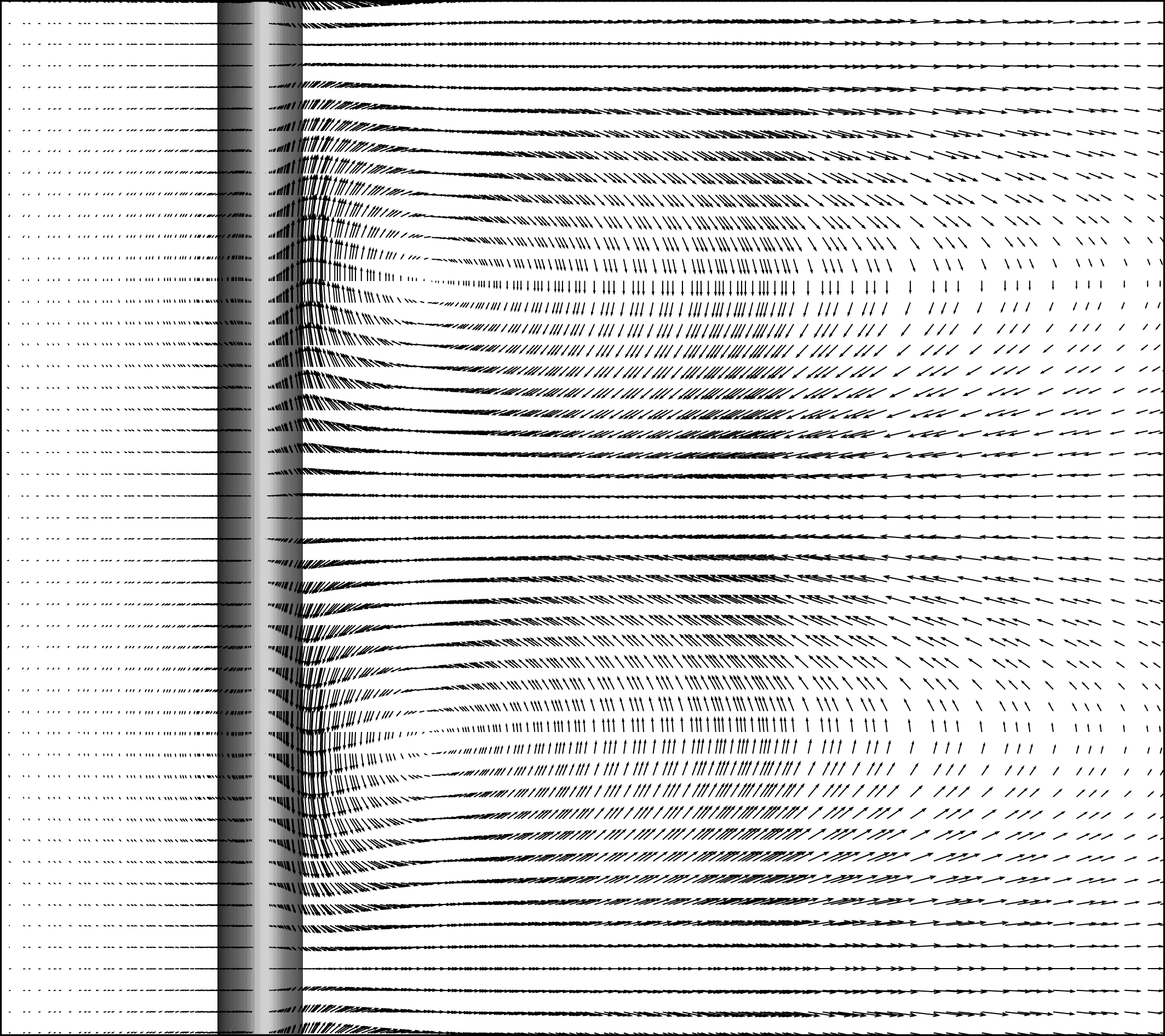
Top down view of the 3-D steady flow at
 $Re=60$
and
 $\unicode[STIX]{x1D706}/d=11$
, depicted through the projected velocity field in the plane grazing the top of the cylinder.

3.1.1 The initial 2-D steady to 3-D steady transition
As indicated above, in contrast to the situation of a cylinder placed in an unbounded flow, the transition to 3-D flow for a cylinder placed near a wall occurs directly from a steady 2-D flow, similar to the situation for a backward-facing step (Barkley, Gomes & Henderson Reference Barkley, Gomes and Henderson2002). As with that flow, its perturbation mode takes the form of periodic cells evenly distributed along the span of the cylinder. Figure 5 shows the perturbation velocity field projected into the plane just touching the top of the cylinder for
 $Re=60$
and
 $\unicode[STIX]{x1D706}/d=11$
taken when the 3-D instability begins. This clearly shows the rotating cells associated with this instability mode. Stability analysis on the steady base flow shows that the onset of 3-D flow first occurs at
 $Re_{c,3D}=36.8$
for a spanwise wavelength
 $\unicode[STIX]{x1D706}_{c}$
of
 $8.6d$
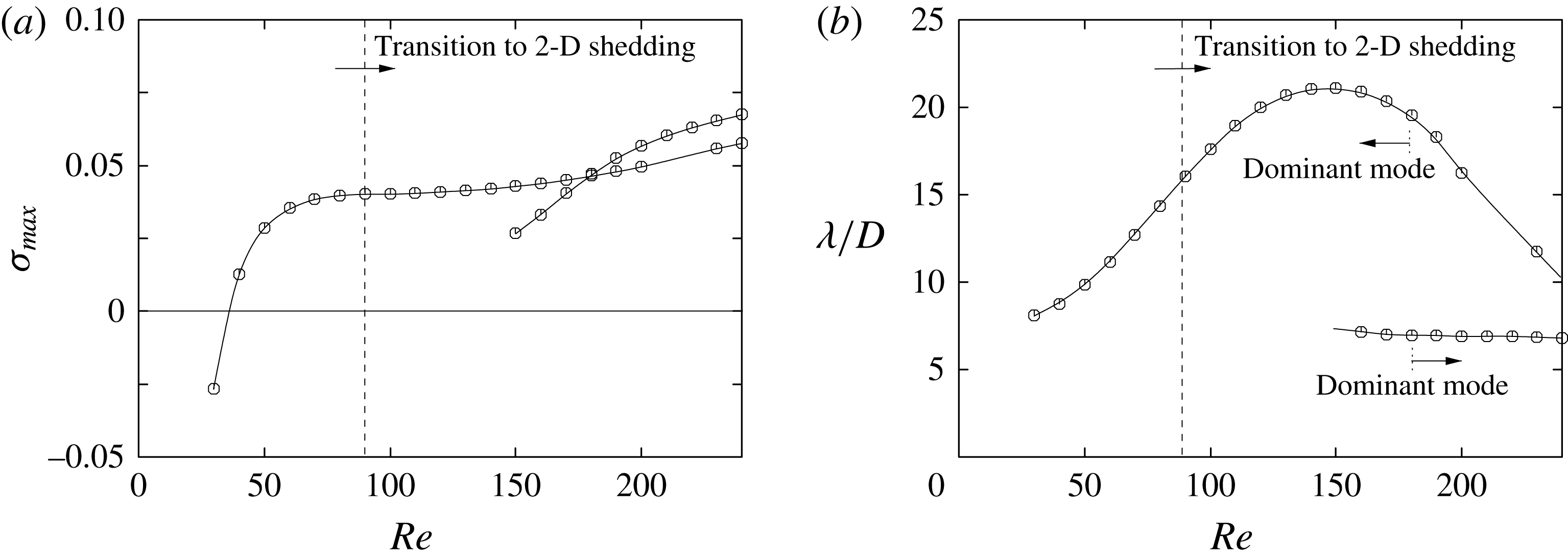
. Figure 6 shows that the maximum observed growth rate saturates by
 $Re\sim 60$
, only increasing further beyond
 $Re\sim 150$
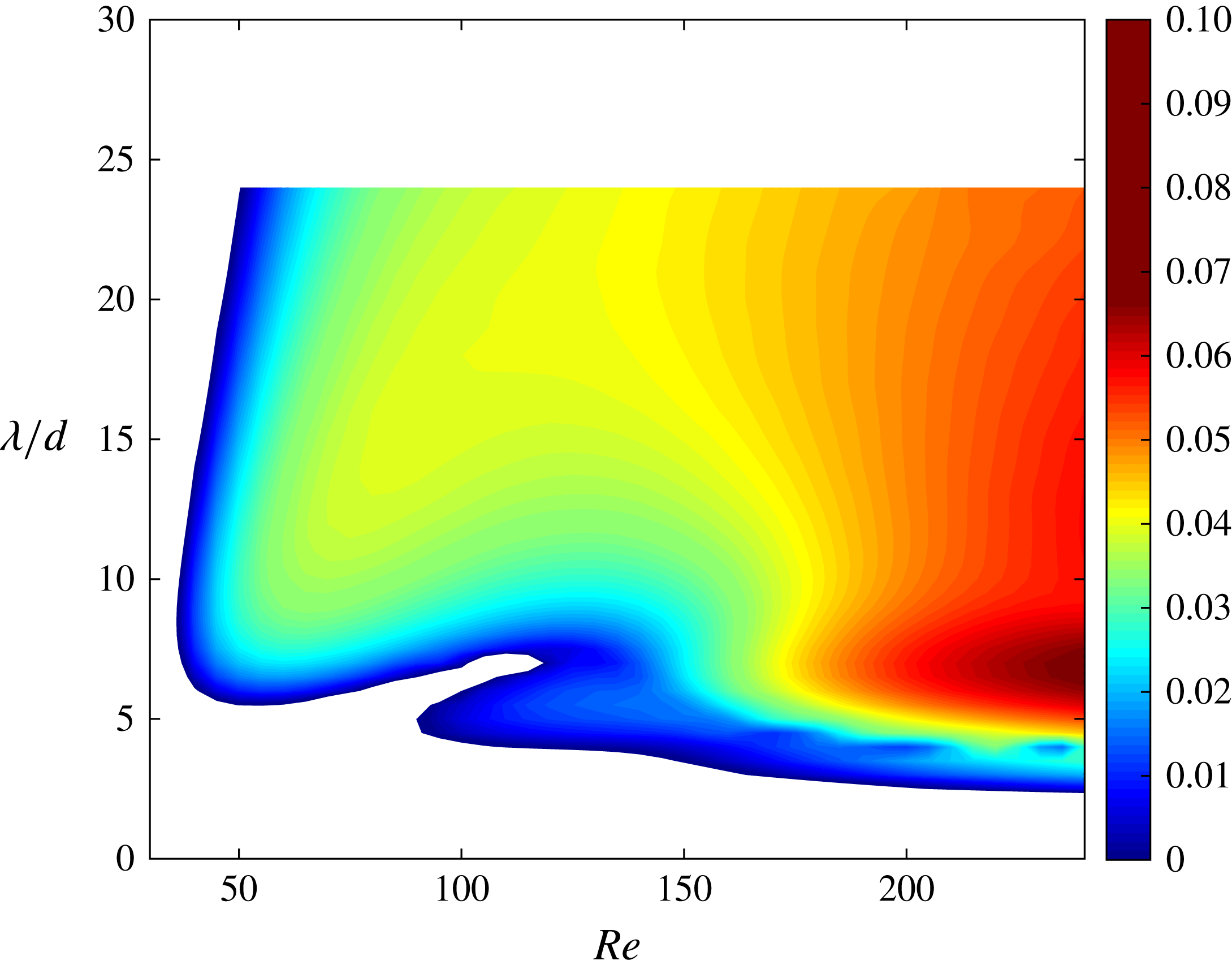
, well beyond the onset of shedding. This is further confirmed in figure 7, where the growth rate is reported over the entire range of Reynolds numbers and spanwise wavelengths. The white regions in this figure represent negative growth rates and therefore stable wakes. Growth rates that are not real and are instead composed of a complex conjugate pair (i.e. the period of the mode is different from that of the base flow) were only detected in the blue region comprised between
 $90\lesssim Re\lesssim 150$
and
 $5\lesssim \unicode[STIX]{x1D706}/d\lesssim 8$
. The base flows for this analysis were generated using a steady version of the spectral-element code, allowing the stability to be investigated well beyond the transition to unsteady flow. The preferred wavelength can be seen to increase from
 $\unicode[STIX]{x1D706}=8.6d$
at onset to reach values in excess of
 $20d$
at
 $Re=150$
, before suddenly dropping back on further increasing the Reynolds number. This is associated with the growth rate versus wavelength curves for
 $Re\gtrsim 150$
developing two peaks, with the lower-wavelength peak dominating for
 $Re\gtrsim 180$
.
(a) Maximum growth rate of the most unstable mode for transition from 2-D steady to 3-D steady flow. (b) Variation of the wavelength of the fastest growing mode with the Reynolds number. Beyond
 $Re\sim 150$
there are two peaks in the growth rate curve with the shorter-wavelength peak developing the higher amplitude for
 $Re\gtrsim 180$
.

Contour map of the growth rate
 $\unicode[STIX]{x1D70E}$
as a function of the Reynolds number
 $Re$
and the wavelength
 $\unicode[STIX]{x1D706}/d$
for the 2-D steady to 3-D transition. For most of the domain, the dominant 3-D mode is steady, except for a small (blue) region centred around
 $Re=120$
and
 $\unicode[STIX]{x1D706}/d=5$
and extending to higher Reynolds numbers.

3.1.2 Transition to 2-D unsteady flow
The transition from steady to unsteady 2-D flow occurs when the recirculation bubble at the rear of the cylinder becomes unstable and starts to shed vortices (figure 4 b). These vortices interact with the wall through the no-slip condition, generating secondary vorticity as they advect downstream. In turn, this secondary vorticity is pulled away from the wall to combine with the primary generating vortex to form a vortex pair. The self-induced velocity of the pair causes it to move upwards and away from the wall, but because the primary vortex is stronger, the movement is along a curved path. The essential features of this process can be seen in figure 4(b).
The structure of the perturbation field at
 $Re=Re_{c,2D}$
depicted using perturbation spanwise vorticity with overlaid base flow vorticity contours at
 $\pm 0.1U/d$
.

(a) Growth rate of most unstable mode from stability analysis applied to the rolling cylinder for
 $50\leqslant Re\leqslant 200$
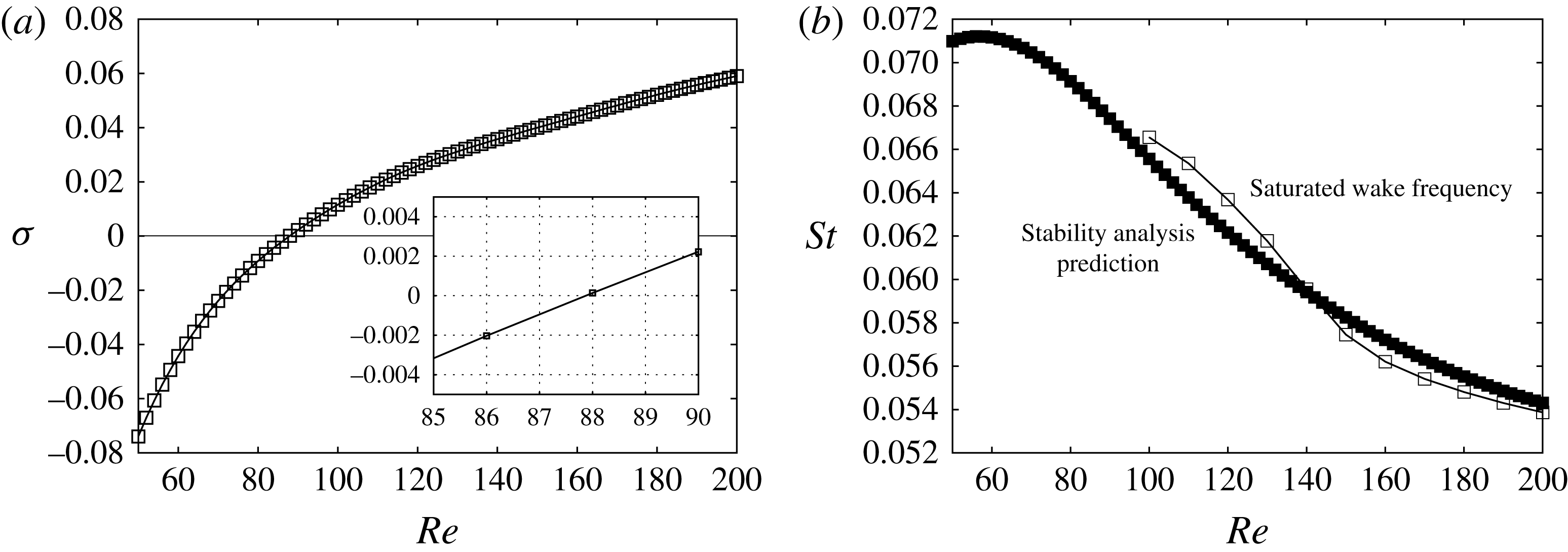
. The lower inset shows the stability curve as it crosses the neutral stability line. (b) Predicted Strouhal number of the perturbation field compared to that of the saturated flow state.

Figure 8 shows the form of the instability mode visualised by the perturbation spanwise vorticity, indicating that the mode has large amplitude where the base vorticity field is strong as well as close to the ground plane. Linear stability analysis of the steady base flow shows that this transition, which is characterised by a Hopf bifurcation, occurs at
 $Re_{c,2D}\simeq 88$
. This is shown in figure 9, which gives the growth rate and the preferred oscillation frequency as a function of the Reynolds number. Although not shown in the paper, it was verified that the fluctuating lift oscillation amplitude varied as
 $\sqrt{(Re-Re_{c,2D})}$
close to the transition, as expected for a Hopf bifurcation. The oscillation frequency decreases with Reynolds number from
 $St\simeq 0.066$
at onset to 0.054 at
 $Re=200$
. Interestingly, the frequency of the fully saturated 2-D wake stays relatively close to the perturbation mode frequency over this entire range. This is perhaps surprising given that the saturated periodic state deviates considerably from the steady wake base state, but it is probably an indication that the frequency selection is based on the separating shear-layer properties rather than the near-wake field. Discussion on frequency selection for the related case of a cylinder in free stream can be found in Pier (Reference Pier2002), Barkley (Reference Barkley2006), Sipp & Lebedev (Reference Sipp and Lebedev2007), Leontini, Thompson & Hourigan (Reference Leontini, Thompson and Hourigan2010).
3.1.3 Stability of the fully developed 2-D periodic wake
Given the discussion in § 2.1, it seems likely that the initial 3-D development of the wake at a particular Reynolds number above
 $Re_{c,U}=88$
will be determined by the stability of the 2-D periodic flow. That will be tested in later sections through direct simulations. In this section, the 3-D linear stability of the 2-D periodic base flow is characterised first.
Contour map of the dominant growth rate
 $\unicode[STIX]{x1D70E}$
as a function of the Reynolds number
 $Re$
and the wavelength
 $\unicode[STIX]{x1D706}/d$
for the 2-D periodic base flow.

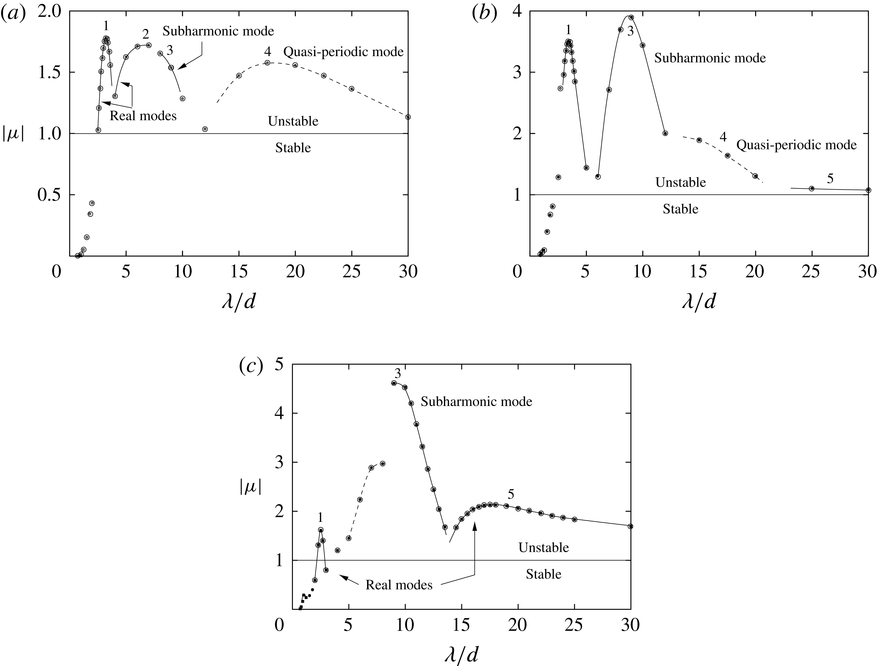
Floquet multiplier variation against spanwise wavelength for the dominant Floquet mode at each wavelength for
 $Re=100$
(a),
 $Re=130$
(b) and 160 (c).

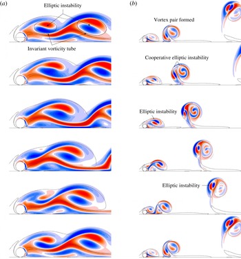
Evolution of the spanwise perturbation vorticity for the mode 1 of figure 11 at
 $Re=100$
(a) and
 $Re=160$
(b), overlaid with the base flow vorticity contours at
 $\pm 0.1U/d$
. The images are
 $1/5$
of a period apart. The spatial distribution of the instability fields show strong signs of elliptic instability of the vortex cores, as discussed in the text.

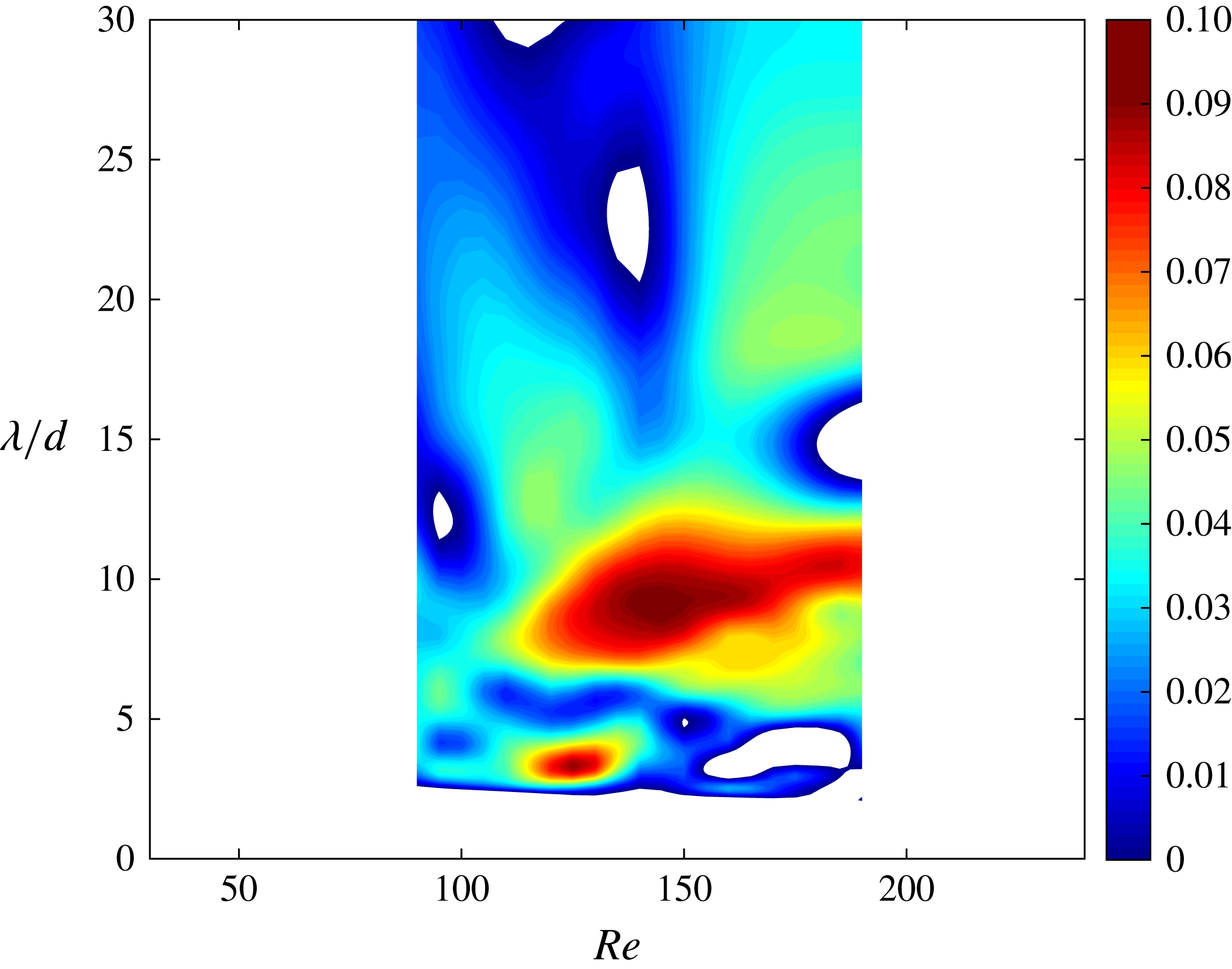
Beyond the transition to unsteady flow, a number of different modes contribute to the wake becoming three-dimensional. The occurrence and growth rates of these modes are also strongly dependent on the Reynolds number, presumably because the structure of the time-dependent 2-D wake is also a strong function of the Reynolds number. Figure 10 summarises the situation by showing the growth rate corresponding to the dominant mode as a contour map over a wide range of spanwise wavelengths and Reynolds numbers beyond
 $Re_{c,2D}$
. There are a few regions of substantial growth, notably corresponding to
 $\unicode[STIX]{x1D706}/d\sim 4$
and
 $8$
–
 $9$
covering different Reynolds number ranges. The picture is a little more complicated than indicated by this map, with local peaks corresponding to different mode types: synchronous modes (i.e. with the same period as the base flow); subharmonic modes (with twice the base period); and quasi-periodic modes (with periods different from the base period). To show this in more detail, Floquet multiplier variations as a function of wavelength at three different Reynolds numbers
 $Re=100$
, 130 and 160 are given in figure 11. Just above the transition at
 $Re=100$
, the fastest growing mode, marked 1 in the figure, reaches a maximum growth at
 $\unicode[STIX]{x1D706}\simeq 3.2d$
. This corresponds to a real or synchronous Floquet mode, i.e. the period is the same as the base flow period. At this Reynolds number, there are several other contributing modes with positive growth rates covering the wavelength range studied: another real mode 2 with a wavelength of
 $\unicode[STIX]{x1D706}\sim 6$
–
 $7d$
, a subharmonic mode 3 starting at
 $\unicode[STIX]{x1D706}\gtrsim 8d$
and a quasi-periodic mode 4 for
 $\unicode[STIX]{x1D706}\gtrsim 15d$
. These all have strongly positive growth rates, although less than the short-wavelength mode 1. At
 $Re=130$
, the short-wavelength mode 1 is still present, but now the most dominant mode is the subharmonic mode 2 at a wavelength of
 $\unicode[STIX]{x1D706}\simeq 9d$
. The longer-wavelength quasi-periodic mode is still present, although it gives way to another real mode at still higher wavelengths (
 $\unicode[STIX]{x1D706}\gtrsim 25d$
). At
 $Re=160$
, there are again several changes to the picture. The short wavelength mode 1 and subharmonic mode 3 are still present, with the subharmonic mode relatively much more dominant. At higher wavelengths (
 $\unicode[STIX]{x1D706}\gtrsim 15$
), a real mode 5 becomes more dominant than the quasi-periodic mode 4 over that wavelength range. The fact that all these modes are amplified and they cover a wide wavelength range suggests that the wake is likely to become chaotic quickly after the initial growth of the most dominant mode begins to saturate. This is investigated further using direct numerical simulations in the following section, but prior to this, the vorticity structure of the modes is examined.
Figure 12 shows the evolution of the perturbation spanwise vorticity field for mode 1 at
 $Re=100$
, where it is the fastest growing mode, and at
 $Re=160$
, where it is less dominant. Especially in the lower Reynolds number case, the structure of the perturbation field inside the newly formed and shed vortex cores clearly shows the characteristics of elliptical instability (Bayly Reference Bayly1986; Pierrehumbert Reference Pierrehumbert1986; Landman & Saffman Reference Landman and Saffman1987; Waleffe Reference Waleffe1990; Leweke & Williamson Reference Leweke and Williamson1998; Thompson et al.
Reference Thompson, Leweke and Williamson2001b
; Kerswell Reference Kerswell2002). In particular, the perturbation vorticity shows two lobes of positive and negative vorticity, whose extrema align at
 ${\sim}45^{\circ }$
to the main axes of the elliptically shaped vortex cores (marking regions with elliptic streamlines in the reference frame moving with the advection velocity at the centres of these cores. Also importantly, the orientation of the lobes is approximately maintained as the vortices advect downstream, allowing the perturbation to grow and allowing feedback from one shedding cycle to the next. Although somewhat far from the idealised cases for which the theory was developed (Waleffe Reference Waleffe1990), for finite-sized vortices, the preferred wavelength is dependent on the core size. Le Dizès & Laporte (Reference Le Dizès and Laporte2002) showed that for Gaussian vortices under strain, the spanwise wavelength is given by
 $\unicode[STIX]{x1D706}=2.78a$
, with
 $a$
the Gaussian length scale. For highly strained vortices, such as is the case here, the appropriate length scale (
 $a$
) is given by Le Dizès & Verga (Reference Le Dizès and Verga2002) as
 $a^{2}=(a_{M}^{2}+a_{m}^{2})/2$
, with
 $a_{M}$
and
 $a_{m}$
corresponding to the semi-major and minor axis lengths, respectively. At
 $Re=100$
, figure 12 shows that the approximately invariant vorticity tube grows in size as the vortex cores advect downstream. For the first image, where the elliptical instability pattern is first recognisable, the length scales from the just formed and downstream cores obtained by fitting Gaussian profiles to the major and minor axes are
 $\simeq 0.95d$
and
 $1.27d$
, giving preferred spanwise wavelengths of 2.7 and
 $3.5d$
, respectively. Figure 11 shows that Floquet analysis indicates that the maximum growth for this mode corresponds to a wavelength of
 $\unicode[STIX]{x1D706}=3.2d$
, near the centre of the range of the theoretical prediction. At
 $Re=160$
, Floquet analysis shows the preferred wavelength of mode 1 drops to
 $\simeq 2.5d$
. This is in line with the prediction of the more compact shed cores due to lower viscous diffusion at the higher Reynolds number. In this case, an asymmetrical counter-rotating vortex pair is formed before the newly formed vortex advects very far downstream. This composite structure also shows evidence of a perturbation pattern consistent with elliptic instability, as it advects away from the wall in an approximately circular arc. Various studies have identified elliptic instability in an isolated counter-rotating vortex pair (e.g. Leweke & Williamson Reference Leweke and Williamson1997).
Figure 13 shows the perturbation streamwise vorticity structure of modes 3 and 5 at
 $Re=160$
. Mode 3, the shorter-wavelength mode, is subharmonic, repeating every two base flow periods. Mode 5 only becomes dominant for
 $Re\gtrsim 160$
. Below this Reynolds number, a quasi-periodic mode occupying this wavelength range has a higher growth rate. Interestingly, the amplitude distributions of these two modes appear similar. Inside the newly forming vortex, the distributions broadly match between the two modes, in terms of both the sign and distribution of perturbation vorticity. The vorticity distributions within the downstream vortex pairs are also similar, but of opposite sign, as is the case with the layer of vorticity near the ground between the two main vortical structures.
The physical nature of the instability in this case is more difficult to discern. The developing wake does not form a series of relatively long-lived elliptical-shaped vortices in this case, but rather a newly formed vortex generates secondary vorticity beneath it, which is subsequently drawn away from the boundary to form an unequal strength counter-rotating vortex pair. The process is shown in figure 14. This indicates that there are a number of different identifiable vortex structures and groupings that combine to lead to the observed flow instability modes.
Visualisations of the streamwise perturbation vorticity for subharmonic mode 3 (a) and real mode 5 (b) at
 $Re=160$
. These images depict streamwise perturbation vorticity coloured contours with base flow vorticity contour line at
 $\pm 0.1d/U$
overlaid to highlight the locations of the vortices.

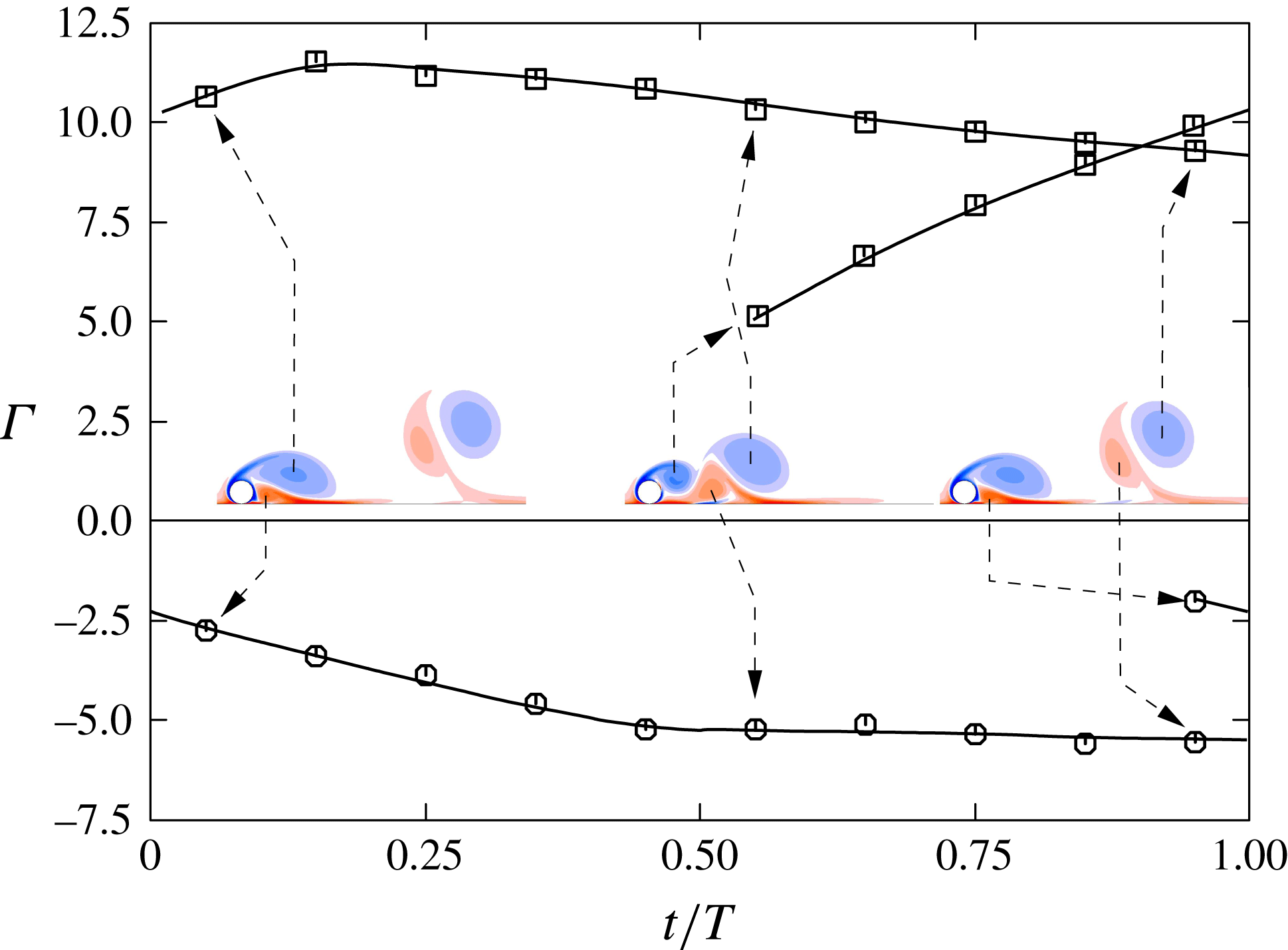
The evolution of the circulation in the primary and secondary vortices as they advect downstream is shown in figure 15. The primary (clockwise) vortices that directly form from the separating shear layer, grow quickly in strength prior to the shear layer pinching off and releasing the vortices to move downstream. The circulation then slowly decays. During its initial growth and soon after its release, this primary vortex combines with the secondary vorticity generated at the boundary, to form the vortex pair. At a point in time when this pair becomes unambiguously defined, i.e. between images 2 and 3 of figure 14, the ratio of circulations between the component vortices of the pair is approximately
 $-2:1$
. So, Ryan & Sheard (Reference So, Ryan and Sheard2011) analysed the stability of unequal strength Lamb–Oseen vortices, which have a Gaussian vorticity distribution, examining how the growth rate and preferred wavelength varied with circulation ratio. Such a system is subject to both the short-wavelength elliptic instability and the longer-wavelength Crow instability. The results of So et al. (Reference So, Ryan and Sheard2011) can be used to obtain an estimate for the most unstable wavelength. A recent review of the Crow instability is given in Leweke, Dizès & Williamson (Reference Leweke, Dizès and Williamson2016). Examining the spanwise perturbation vorticity field of mode 5 (not shown) shows the characteristic lobe structure of Crow instability in the vortex pair as it moves away from the cylinder and the wall. By approximating the vorticity distributions within the pair at formation in terms of a sum of Gaussian distributions to extract the length scale for each vortex, together with the overall circulation ratio, a preferred wavelength of approximately
 $\unicode[STIX]{x1D706}\simeq 20d$
can be predicted from the work of So et al. (Reference So, Ryan and Sheard2011). This is close to the observed preferred wavelength of mode 5 at
 $Re=160$
of
 $\unicode[STIX]{x1D706}\simeq 18d$
. However, in this case, the perturbation field does not grow as the vortex pair advects, so the Crow instability of the pair alone cannot be responsible for the maintenance of the instability mode from one cycle to the next. At best, this could suggest that the Crow instability plays a role in wavelength selection of the overall global instability.
During the formation and evolution of the wake vortices, it is also possible to take into account the image vortices, linked to the presence of the wall and symmetrically located with respect to it. The near wake vortex pair and its image form a symmetric four-vortex system, a configuration analysed previously in the context of aircraft trailing wakes (e.g. Crouch Reference Crouch2005; Jacquin et al. Reference Jacquin, Fabre, Sipp and Coustols2005; Winckelmans et al. Reference Winckelmans, Cocle, Dufresne and Capart2005). The existence of short-wave (elliptic) and Crow-type long-wave instabilities was also found in these systems. Although the identification of such systems is transitory for this wake, is seems plausible that the Crow instability would play a role in the global 3-D instability and wavelength selection for the wake.
Evolution of the spanwise wake vorticity at
 $Re=160$
showing the formation of new vortices from the separating shear layer, generation of secondary vorticity at the boundary and release into the wake, and the formation of counter-rotating vortex pairs that self-propel away from the wake as the pair moves downstream. Images are separated in time by
 $1/5$
of a period.

Evolution of the circulation
 $\unicode[STIX]{x1D6E4}$
of the primary and secondary vortices over a shedding cycle as they form and advect downstream. Here,
 $Re=160$
.

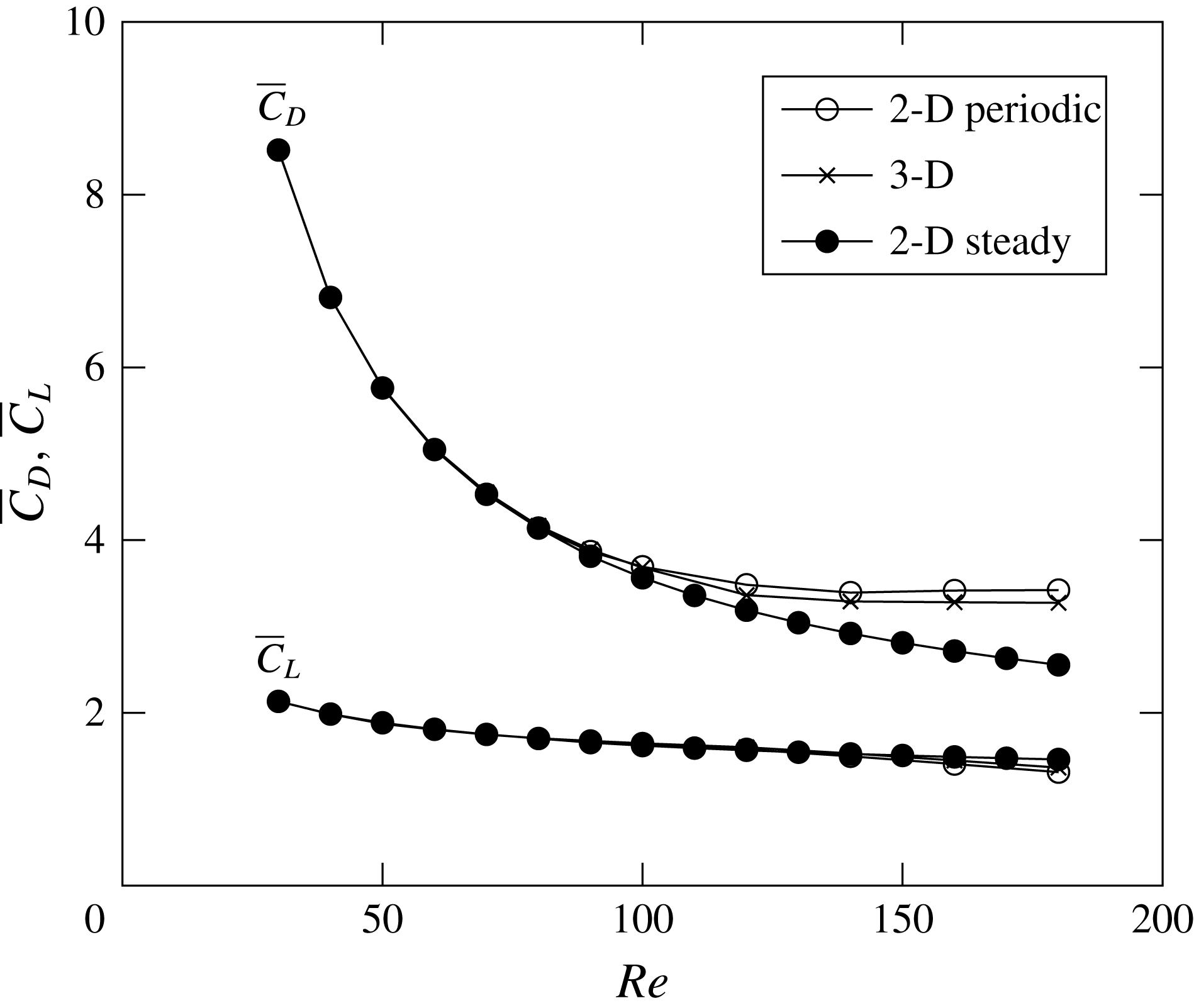
Comparison of time-averaged body force coefficients, drag
 $\overline{C}_{D}$
and lift
 $\overline{C}_{L}$
, between the two- and three-dimensional simulations for
 $30\leqslant Re\leqslant 180$
. Note that beyond
 $Re_{c,2D}$
the 2-D steady predictions shown by the filled circles are based on flows calculated with the steady solver.

3.2 Saturated 3-D state
3.2.1 Computed forces
In this section the force coefficients after the flow has reached its fully saturated 3-D state are compared with predicted force coefficients from 2-D steady and periodic simulations. The time-mean forces computed obtained from 3-D direct numerical simulations are in good agreement with the 2-D ones. Figure 16 shows plots of the mean drag and lift coefficients, as defined in 2.3, versus the Reynolds number. For Reynolds numbers up to the Hopf bifurcation leading to a periodic 2-D state, the 2-D and 3-D curves are effectively indistinguishable. This is consistent with the relatively weak effect on the wake of the steady 3-D instability even as it saturates, as shown in figure 17. However, even beyond the transition to periodic flow, the difference between the 2-D periodic and 3-D predictions remains small, and is limited to be less than 5 % for the mean drag coefficient and 4 % for the lift coefficient at the highest Reynolds number considered here of
 $Re=180$
. In this case, the saturated 3-D wake is distinctly different from the 2-D periodic wake, as is explored further below. The figure also shows the lift and drag coefficients based on the steady flow for
 $Re>Re_{c,2D}$
obtained from the steady solver. These curves deviate considerably from the other two sets as the Reynolds number increases. This is consistent with the increasingly elongated recirculation region of the steady flow deviating further from the near-wake vortex shedding of the 2-D periodic and 3-D flows as the Reynolds number is increased.
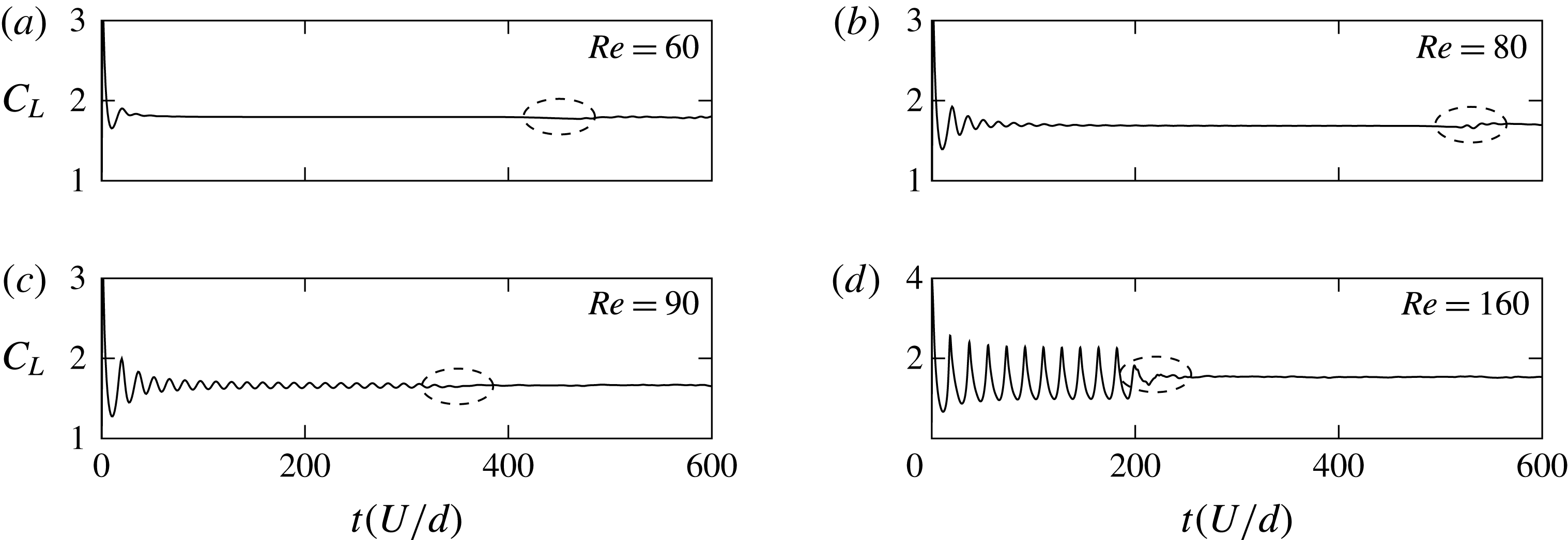
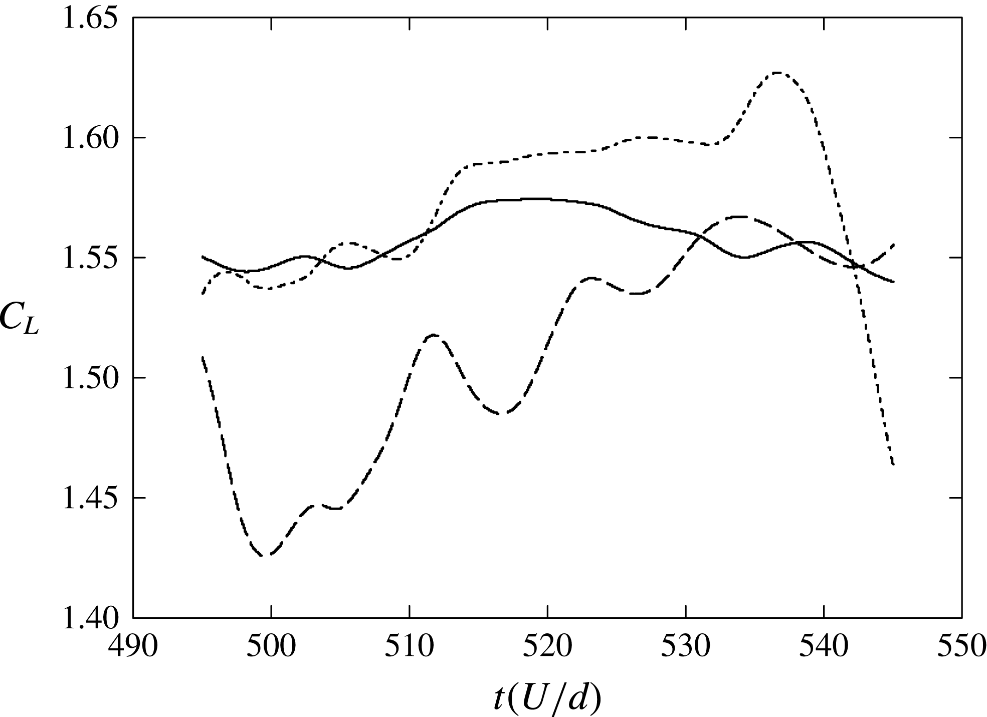
Figure 18 shows the temporal evolution of the lift coefficient obtained from full 3-D simulations at
 $Re=60,\,80,\,90$
and
 $160$
. The initial evolution follows the one observed from the 2-D simulations (figure 2) until the 3-D instability grows sufficiently to change the 2-D structure of the flow. This effect can be seen in the temporal development of the lift coefficient: below the Hopf bifurcation at
 $Re_{c,2D}=88$
, the 3-D transition disturbs the otherwise constant lift coefficient at approximately
 $t=400-600U/d$
(upper two plots), whilst beyond the 2-D transition, the periodic oscillations in the curves die out at approximately
 $t=200-400U/d$
(bottom two plots) as a result of the 3-D instability reaching a sufficient amplitude to substantially alter the otherwise 2-D periodic flow.
It is of interest why the oscillations in the lift signal are substantially suppressed once the wake reaches its saturated 3-D state. To investigate this, sectional lift coefficient signals, i.e. the lift coefficient per unit span at a particular spanwise position, were examined at different points across the span. Figure 19 shows the evolution of the lift signals at two points separated by half the span width (dashed lines) together with the mean lift signal (solid line), for
 $Re=160$
in the saturated state. Clearly, there is a significant variation in the local lift coefficient across the span, indicating that the underlying 2-D vortex shedding is uncorrelated. In addition to this, even the sectional lift coefficients are not very periodic. This is consistent with a change from strong, regular 2-D shedding of vortices initially to a much more disordered 3-D wake without a strong underlying 2-D periodic vortical wake structure. Note that for these simulations, a low-level white-noise perturbation of amplitude
 $10^{-4}U$
was added to each velocity component at startup to accelerate the development of the three-dimensionality.
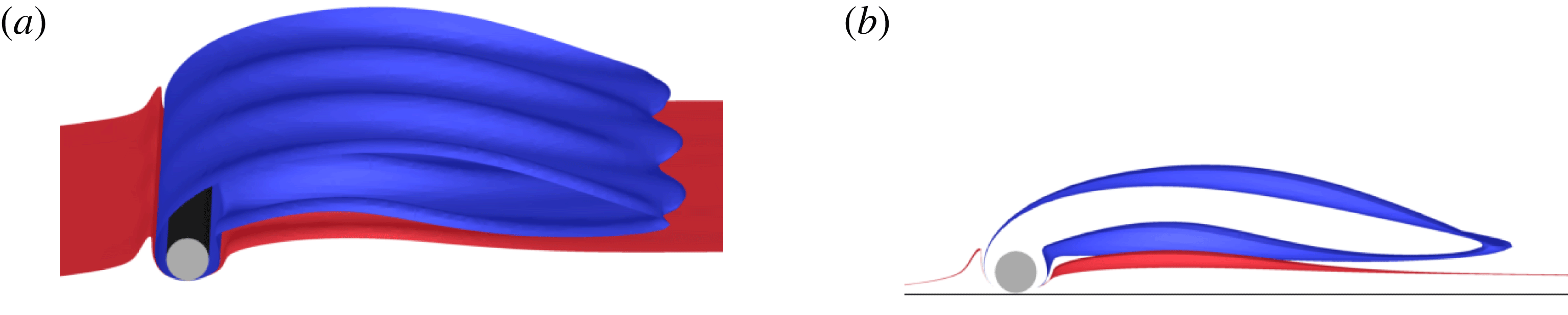
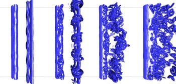
The fully developed wake state at
 $Re=50$
visualised over a spanwise distance of three characteristic wavelengths. The wake state is depicted using an isosurface of the spanwise vorticity (
 $\unicode[STIX]{x1D714}_{z}=\pm 0.5$
). (a) Perspective view. (b) Side view.

Temporal evolution of the lift coefficient from
 $Re=60$
to 160 computed from the 3-D direct numerical simulations. The dashed ellipses show the instant at which the 3-D instability has grown sufficiently to alter the 2-D flow.

Evolution of the sectional lift coefficient at two spanwise locations (dashed lines) separated by half the span width at
 $Re=160$
in the fully saturated state. The spanwise-averaged lift coefficient is also shown by the solid line. The period corresponding to 2-D vortex shedding is approximately 20 units.

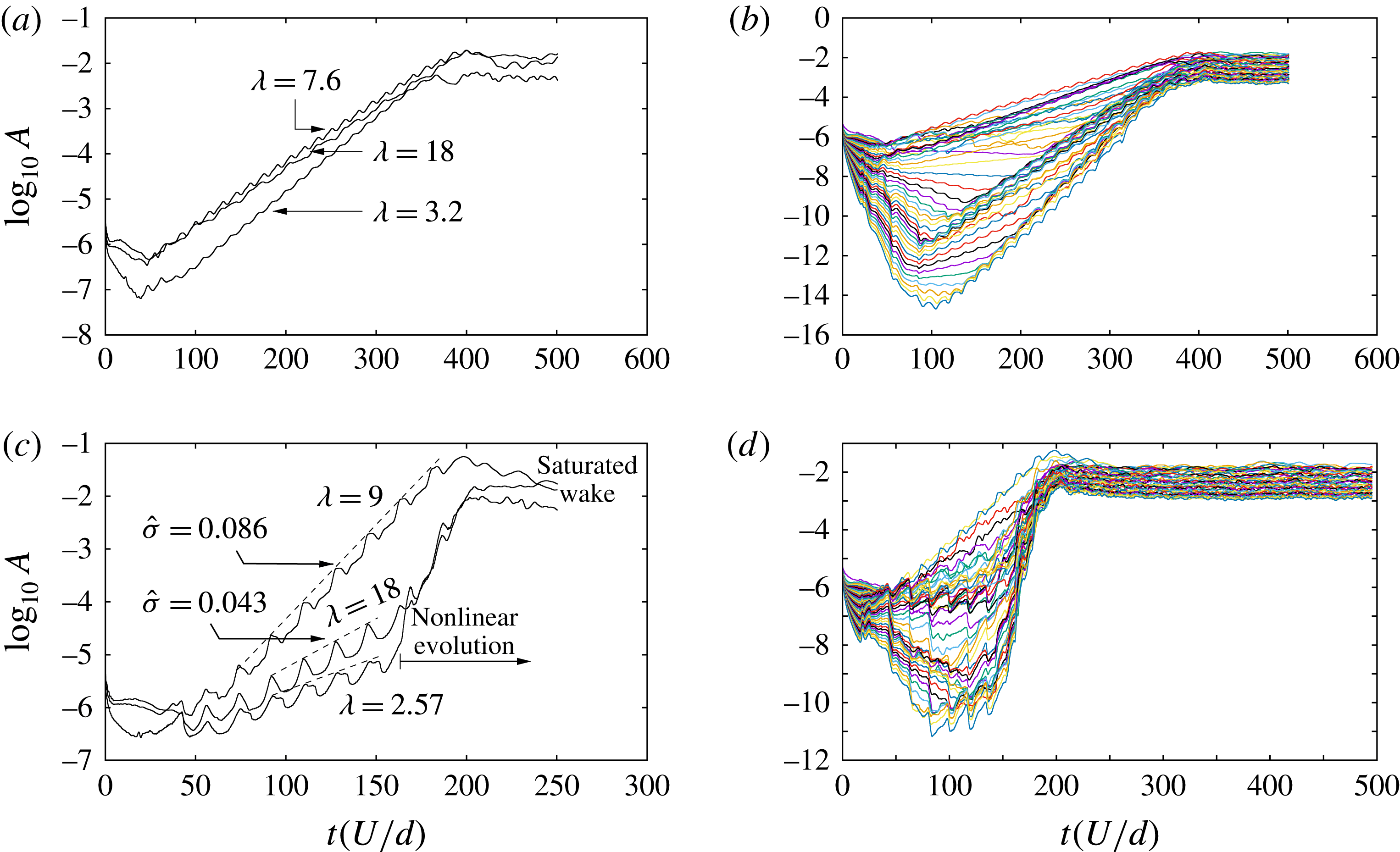
Evolution of the amplitude of spanwise Fourier modes at different Reynolds numbers. Top row:
 $Re=100$
; bottom row:
 $Re=160$
. The panels on the left show the evolution of the three dominant wavelengths as predicted by Floquet analysis, and those on the right show the evolution of the amplitudes corresponding to the first 48 modes. The simulations are started impulsively, with a low-level white noise to accelerate the development of the three-dimensionality. Measured slopes of the evolution curves in the linear regime give estimated growth rates (
 $\hat{\unicode[STIX]{x1D70E}}$
) in agreement with growth rate predictions from Floquet analysis given in figure 11.

3.2.2 Development and saturation of 3-D flow
Within the steady regime (
 $Re<Re_{c,2D}$
), the evolution to a fully evolved 3-D wake for
 $Re>Re_{c,3D}$
leads to the 2-D spanwise vorticity isosurfaces becoming wavy in the spanwise direction, with little alteration to the main underlying 2-D structure of the flow. As identified above, this effect can be seen on figure 17(a), and the extent of this deformation on figure 17(b). These predictions are consistent with those made by Stewart et al. (Reference Stewart, Thompson, Leweke and Hourigan2010), who in addition conducted experiments in a water channel. Their experiments showed that the results of the experimental streaklines and of the predicted 2-D flow are in good qualitative agreement, at least while the three-dimensionality is developing. Note that the final saturated state in this case is weakly unsteady. For instance, at
 $Re=45$
there is a low-level oscillation leading to the weak shedding of vorticity into the wake, while the global 3-D structure shown in figures 5 and 17 is maintained. For Reynolds numbers beyond the transition to vortex shedding, which is the main focus here, direct numerical simulations of the flow indicate that, prior to its settling into its final state, the flow initially undergoes a rapid transition to 2-D vortex shedding, as indicated by the lift trace curves of figure 18. The numerical method involves representing the spanwise variation through a Fourier decomposition, hence the evolution of the spanwise modes can be easily extracted. A convenient measure of the amplitude of each mode is provided by the root mean square (r.m.s.) amplitude of the spanwise velocity component of each complex Fourier mode, since that velocity component is zero prior to 3-D flow development. Specifically, the evolution of the modal amplitudes (
 $A_{n}$
), computed as a r.m.s. spatial average over all 2-D node points (
 $N_{xy}$
) of the moduli of the
 $z$
-velocity complex Fourier coefficients (
 $a_{n}$
) corresponding to mode index
 $n$
, i.e.
 $$\begin{eqnarray}A_{n}(t)=\sqrt{\left(\frac{1}{N_{xy}}\mathop{\sum }_{i=1}^{N_{xy}}\left|a_{n}^{i}(t)\right|^{2}\right)},\end{eqnarray}$$
are shown in figure 20 for
 $Re=100$
and
 $Re=160$
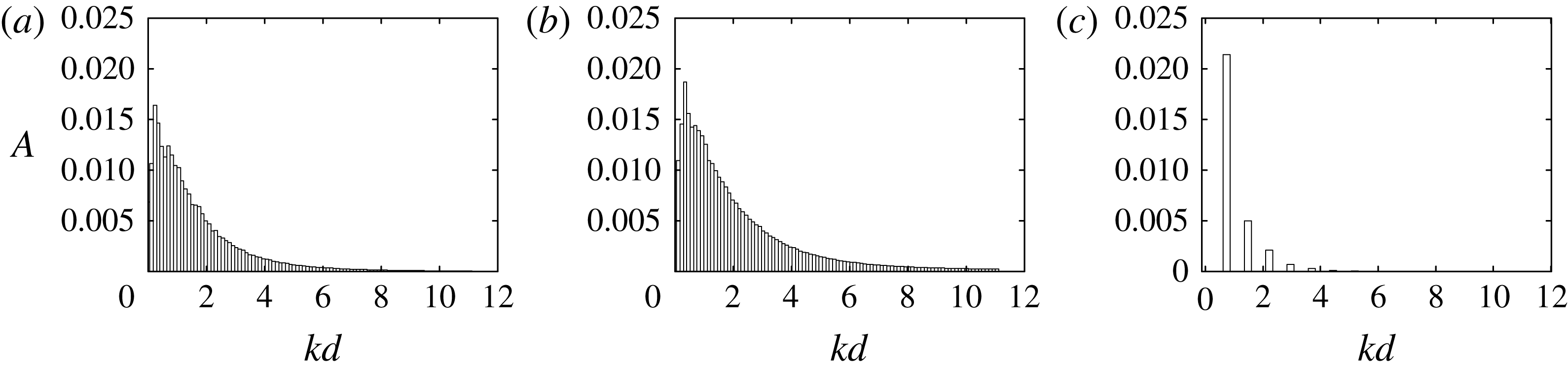
. The two figures in the left column show the development of modes corresponding to key wavelengths identified by the global stability analysis. Indeed, after an initial period over which the dominant mode for each wavelength emerges, the growth rates as measured by the slopes of the curves over many oscillation periods have values consistent with the linear stability analysis predictions. At some point in time, the modes grow sufficiently to begin to saturate nonlinearly, leading the flow to reach its asymptotic state. After saturation, the figures in the right column show that the final state is influenced by many modes of different wavelengths, suggesting a rapid transition to fully chaotic flow. Figure 21 shows time-mean r.m.s. amplitudes of each Fourier mode taken over the last 100 time units (in the fully saturated state) at (a)
 $Re=100$
and (b)
 $Re=160$
. Here, the horizontal axis is the non-dimensional wavenumber
 $kd$
. These spectra can be compared with figure 21(c) at
 $Re=45$
, where the saturated state shows a single spectral peak corresponding to
 $kd=0.74$
(or
 $\unicode[STIX]{x1D706}/d=8.5$
) together with harmonics accounting for the distortion of the saturated final state from the pure sinusoidal linear instability mode. For the two higher Reynolds number cases, the spectra are continuous as a result of the nonlinear interactions between modes, and this is indicative of a chaotic final wake state. Indeed, the modes corresponding to the dominant linear instability mode numbers do not dominate the spectra at saturation.
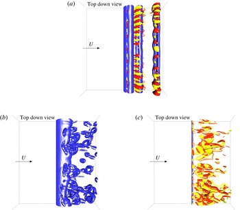
Isosurface plots taken at key points in the flow development help elucidate the wake development. Figure 22(a) shows an isosurface of
 $Q=0.01$
at
 $t=350d/U$
. The
 $Q$
-criterion is a vortex identification method defined initially by Hunt, Wray & Moin (Reference Hunt, Wray and Moin1988). This isosurface is merged with isosurfaces of positive/negative streamwise vorticity to highlight the dominant spanwise mode at a time when the three-dimensionality is beginning to modify the otherwise 2-D wake structure. In this case,
 $Re=100$
. The wavelength of the streamwise vorticity pattern extracted from this image is consistent with the short-wavelength mode 1 instability prediction (figure 22
a) from stability analysis. Soon after, the wake develops nonlinearly, with a typical snapshot shown in figure 22(b).
Time-mean amplitudes of saturated Fourier modes corresponding to the spanwise velocity component against dimensionless wavenumber
 $kd$
for (a)
 $Re=100$
and (b)
 $Re=160$
. These are taken over the 100 time units after the asymptotic state is reached. The right-hand image (c) shows the final mode amplitude distribution for
 $Re=45$
, well below the transition to the periodic state.

Evolution of the wake at
 $Re=100$
from direct simulations. (a) Isosurface of
 $Q=0.01$
(blue) highlighting the predominantly 2-D vortices, with isosurfaces of streamwise vorticity at
 $\unicode[STIX]{x1D714}_{x}=\pm 0.1$
(red/yellow) superimposed. At this time (
 $t=350d/U$
), the 3-D instability modes have grown sufficiently to begin to affect the wake. (b,c) At
 $t=500d/U$
, after the flow has fully saturated. The wake is complex and chaotic with many 3-D wavelength components contributing. The isosurface corresponding to
 $Q=0.01$
is plotted in panel (b) and the isosurfaces of streamwise vorticity at
 $\unicode[STIX]{x1D714}_{x}=\pm 0.1U/d$
in panel (c).

Stages in the evolution of the wake at
 $Re=160$
as depicted by isosurfaces of
 $Q=0.01$
. The first three images show the wake structure for three consecutive cycles just after the three-dimensionality is starting to modify the flow. The final image is a typical image after the flow has reached its asymptotic state.

At a higher Reynolds number of
 $Re=160$
, the development is somewhat different. Figure 23 shows a sequence of wake states from the time that three-dimensionality is beginning to develop. The first three images show the evolution at three consecutive shedding cycles. The three-dimensionality develops quickly, with the spanwise wavelength of the perturbation corresponding to that of mode 3 of figure 11(c). The second image shows substantial distortion of the previously shed 2-D vortex pair, whilst the third image, one cycle later, shows that the subsequently shed vortex pair is virtually destroyed. The final image is a plot taken a few cycles later, after the final asymptotic state is reached. This is similar to the final state at
 $Re=100$
shown in figure 22, except it shows an even more complex finer-scale structure. The previous 2-D periodic wake state is no longer visible at all.
4 Conclusions
The stability analysis of the steady 2-D flow past a cylinder rolling at constant speed along a rigid surface has shown that the key transitions to steady 3-D flow and to periodic vortex shedding occur at
 $Re_{c,3D}=36.8$
and
 $Re_{c,2D}=88$
, respectively. These results are mainly confirmation of findings from a previous study by Stewart et al. (Reference Stewart, Thompson, Leweke and Hourigan2010). However, the main emphasis of this paper is concerned with 3-D wake development in a more realistic configuration, i.e. after a cylinder starts rolling impulsively at a constant velocity, and how this evolution is related to stability theory.
Two main cases can be distinguished. The first is when the Reynolds number is lower than the critical Reynolds number leading to 2-D transition (
 $Re_{c,2D}$
) and above the critical Reynolds number for 3-D steady transition (
 $Re_{c,3D}$
). In this case, the asymptotic flow state is a 3-D flow that is not too far from the prediction based on assuming 2-D flow. Indeed, the drag and lift coefficients are practically unaffected by the three-dimensionality. When the Reynolds number is close to
 $Re_{c,2D}$
, the initially stationary flow develops a few cycles of shedding prior to settling towards a steady state.
The second case is observed for Reynolds numbers above
 $Re_{c,2D}$
. After an impulsive start, the flow undergoes a rapid transition to 2-D periodic shedding. Within a few cycles, e.g. approximately three at
 $Re=90$
and two at
 $Re=160$
, the wake evolves to be close to the periodic state predicted by 2-D simulations. It then continues in this near-periodic state for several cycles, depending on the background noise level. For the cases considered here, this period of evolution was approximately 15 and 10 cycles at
 $Re=90$
and 160, respectively. Stability analysis of the 2-D periodic state, which has not been undertaken previously, then determines the subsequent development of the wake three-dimensionality. At
 $Re=100$
, the wake appears to initially undergo a short-wavelength instability (mode 1 shown in figure 8
a), consistent with an elliptic instability of the shed vortex cores. At longer times, many more spanwise modes come into play and interact nonlinearly, leading to a chaotic final flow state. At a higher Reynolds number of
 $Re=160$
, the initial development of three-dimensionality is different. Here, mode 3 of figure 8(c) is the mode to break two-dimensionality. Again, the wake undergoes a rapid transition to a chaotic final state soon afterwards.
With the noise levels used to initiate the 3-D flow development in the 3-D simulations, the fully saturated wake states take approximately 400 and 200 non-dimensional time units to develop, for
 $Re=90$
and 160, respectively. These values are equivalent to the number of diameters the cylinder rolls whilst maintaining a 2-D state. Although experimental noise levels are likely to be higher, it is still an indication that, after an impulsive start of the cylinder, a 2-D periodic flow state will be maintained for a considerable rolling distance prior to the evolution to a complex 3-D wake. The two- and three-dimensional simulations also show that the mean lift and drag coefficients of the fully saturated 3-D flow are very close to predictions based on 2-D simulations.
It is interesting to speculate whether a similar scenario would apply to a sphere rolling at constant velocity along a wall. In that case, even in free stream, a non-axisymmetric steady transition occurs prior to the periodic transition. The presence of the wall seems likely to cause the premature generation of shedding on impulsive startup, bypassing the slow transition associated with a Hopf bifurcation of a steady flow. However, we will leave this as an open question at this stage.
The numerical model here is essentially an infinite 2-D cylinder forced to roll at constant speed. End effects may play a strong part in the wake evolution, just as it can with the flow past a cylinder away from a boundary. Additionally, if the cylinder is free to roll without any constraints on its movement and velocity, vortex-induced vibrations are likely to occur with an unsteady wake. The simulations and results presented in this paper aim to provide a reference study for the idealised case, and constitute an essential element of an ongoing study concerning the fluid–structure interaction of uniformly and freely rolling bodies translating along a wall.
Acknowledgements
This research was supported under Australian Research Council, Discovery Projects funding scheme DP130100822 and DP150102879. We also acknowledge computing time support through National Computational Infrastructure projects D71 and N67.