1. Introduction
Transition to turbulence in boundary layers is promoted in the presence of external perturbations. In such conditions, the relatively slow natural transition process is bypassed. The final state is a turbulent boundary layer and therefore a higher level of viscous drag. Earlier works have devoted considerable efforts towards the reduction of the high skin friction of the turbulent regime. These studies established the effectiveness of transverse, time-harmonic wall forcing in decreasing wall friction in fully turbulent flows. The present work investigates the influence of such forcing on bypass transition in boundary layers beneath free-stream turbulence.
1.1. Bypass transition in boundary layers
Boundary layer transition to turbulence may be described as a succession of receptivity to external disturbances, growth of primary and secondary instabilities and finally nonlinear breakdown. Two classes of transition have been defined, based on the nature of the primary perturbations. The prevalence of either mechanism, and thus the observed variant of the transition process, largely depends on the spectrum of the initial perturbation field (see e.g. Arnal & Michel Reference Arnal and Michel1990; Saric, Reed & Kerschen Reference Saric, Reed and Kerschen2002).
The first breakdown scenario is commonly known as natural transition and arises in the presence of small-amplitude background perturbations (e.g. Kleiser & Zang Reference Kleiser and Zang1991). This route to turbulence is characterized by the exponential amplification of discrete instability modes, or Tollmien–Schlichting waves, above the critical Reynolds number. At some distance downstream, these two-dimensional waves reach levels of the order of several per cent of the free-stream velocity. At this point, the flow becomes susceptible to three-dimensional secondary instabilities (e.g. Herbert Reference Herbert1988). The subsequent breakdown occurs through the formation of localized turbulent spots (Emmons Reference Emmons1951), which grow in extent and eventually merge to form a continuous turbulent region.
The second class, known as bypass transition, refers to breakdown scenarios that deviate from the above description (see e.g. the reviews by Durbin & Wu (Reference Durbin and Wu2007) and Zaki (Reference Zaki2013)). Initial disturbance growth is dominated by algebraic, or non-modal, amplification, which is active at all Reynolds numbers. The bypass process thus describes a potentially faster path to turbulence than the Tollmien–Schlichting mechanism. Algebraic growth is nevertheless transient and is overcome by viscous decay at finite time. Hence, only perturbations with significant initial magnitude can amplify via the non-modal mechanism and reach sufficient levels to promote laminar–turbulent transition. Studies by Suder, O’Brien & Reshotko (Reference Suder, O’Brien and Reshotko1981) established an initial perturbation amplitude between 0.5 and 1 % as a lower bound for algebraic growth to become the dominant primary amplification mechanism.
While other disturbances such as surface roughness and acoustic waves are potential sources for bypass breakdown, the term ‘bypass’ is commonly associated with transition caused by free-stream vortical perturbations. The bypass process therefore requires a mechanism that allows these external disturbances to enter the boundary layer. Rapid distortion theory (Hunt & Carruthers Reference Hunt and Carruthers1990; Hunt & Durbin Reference Hunt and Durbin1999) and inviscid receptivity studies (Kerschen Reference Kerschen, Reda, Reed and Kobayashi1991) demonstrated that regions of mean shear are shielded from external vortical perturbations – a phenomenon referred to as ‘shear sheltering’. In the presence of viscosity, low-frequency perturbations nonetheless enter the shear (Jacobs & Durbin Reference Jacobs and Durbin1998). This can be explained using a model problem that compares the diffusive time scale for external vortical perturbations to penetrate the boundary layer and the shear time scale (Zaki & Saha Reference Zaki and Saha2009).
Low-frequency vortical disturbances that penetrate the shear trigger a response inside the boundary layer. For example, it was discovered by Dryden (Reference Dryden1936) that external perturbations with amplitudes of the order of a few per cent of the free-stream velocity cause laminar boundary layers to develop ‘speed fluctuations of amplitude considerably greater than that in the free stream’. Taylor (Reference Taylor, Den Hartog and Peters1939) reported the very low frequency of these streaky perturbations, which are dominated by the streamwise velocity component. The works by Klebanoff, Tidstrom & Sargent (Reference Klebanoff, Tidstrom and Sargent1962) and Klebanoff (Reference Klebanoff1971) later brought broader attention to these ‘breathing modes’, which the authors had termed accordingly because of their thinning and thickening effect on the boundary layer. In recognition of these earlier contributions, Kendall (Reference Kendall1985) established the now common terminology of ‘Klebanoff modes’. It should be noted that these ‘modes’ are not eigenfunctions of the governing equations, even though elongated structures like streaks can be considered a general property of shear layers (Phillips Reference Phillips1969).
Landahl (Reference Landahl1975, Reference Landahl1980) explained the origin of streaks in terms of the vertical displacement of mean momentum. This so-called lift-up effect ultimately results from the action of wall-normal velocity perturbations with finite spanwise wavelength on the mean shear of the boundary layer. As a consequence, the mean shear is tilted, which causes the production of normal vorticity and thus a perturbation in the streamwise velocity component. Three-dimensional wall-normal velocity perturbations alone are therefore sufficient for the generation of Klebanoff streaks (see e.g. Breuer & Haritonidis Reference Breuer and Haritonidis1990; Leib, Wundrow & Goldstein Reference Leib, Wundrow and Goldstein1999). Optimal growth studies (Butler & Farrell Reference Butler and Farrell1992; Andersson, Berggren & Henningson Reference Andersson, Berggren and Henningson1999) demonstrated that the optimal spanwise perturbation wavelength is of the order of the local boundary-layer thickness.
Low-frequency streaks, however, do not immediately initiate breakdown. Rather, the regions of increased shear that surround these primary features provide the potential for the development of high-frequency secondary instabilities. Two modes of instabilities are possible (Vaughan & Zaki Reference Vaughan and Zaki2011; Hack & Zaki Reference Hack and Zaki2014). Outer modes are situated on top of boundary-layer streaks and were the dominant type of instability in a number of studies (Jacobs & Durbin Reference Jacobs and Durbin2001; Brandt, Schlatter & Henningson Reference Brandt, Schlatter and Henningson2004; Zaki & Durbin Reference Zaki and Durbin2005). Inner modes become more relevant in the presence of adverse pressure gradients. Beyond the initial growth of the secondary instability, full nonlinear breakdown to turbulence is observed. The resulting spots have opening angles between 18 and 20°, consistent with theoretical (Bowles & Smith Reference Bowles and Smith1995) and experimental studies (Wygnanski, Sokolov & Friedman Reference Wygnanski, Sokolov and Friedman1976; Chong & Zhong Reference Chong and Zhong2005).
1.2. Reduction of turbulent drag by unsteady forcing
For a given Reynolds number, the skin friction of fully turbulent flow is considerably higher than for laminar conditions. An attempt to reduce drag can focus on altering the turbulent state or on delaying the onset of turbulence. In the former category, one mechanism that has received considerable attention is spanwise wall oscillation. The effectiveness of the same mechanism to stabilize the laminar flow regime, and thus delay the onset of turbulence, is examined herein. Therefore, a discussion of the efforts in the context of fully turbulent flow is presented first, followed by some recent efforts in the field of transition delay.
The experimental investigations by Bradshaw & Pontikos (Reference Bradshaw and Pontikos1985) showed a significant decrease in turbulent skin friction as the transverse pressure gradient along a swept wing rapidly changed the direction of the mean flow. Driver & Hebbar (Reference Driver and Hebbar1987) and Spalart (Reference Spalart1989) investigated three-dimensional turbulent boundary layers with continuously changing mean flow direction and noted that the formation of streak-like elongated structures is largely suppressed. In internal flows, Moin et al. (Reference Moin, Shih, Driver and Mansour1990) performed direct numerical simulations (DNS) of channel flow subjected to an impulsively started spanwise pressure gradient. They demonstrated a substantial reduction in the turbulence kinetic energy as the mean flow became strongly three-dimensional. Once the base flow realigned itself in the new direction and became two-dimensional again, the kinetic energy recovered its original level. Jung, Mangiavacchi & Akhavan (Reference Jung, Mangiavacchi and Akhavan1992) simulated turbulent channel flow with spanwise wall oscillation. They demonstrated the continuous reduction of the mean wall shear stress for oscillation periods
 $25<T^{+}<200$
, where
 $T^{+}=Tu_{{\it\tau}}^{2}/{\it\nu}$
and
 $u_{{\it\tau}}$
is the friction velocity.
Baron & Quadrio (Reference Baron and Quadrio1996) investigated the energy budget for oscillatory wall forcing applied to turbulent channel flow. It was shown that the energy savings that result from a reduction in turbulent drag may, for suitable choice of parameters, outweigh the power input into the oscillatory movement so that a net energetic gain is achieved. A comprehensive review of turbulent flows under the influence of transverse forcing is given by Karniadakis & Choi (Reference Karniadakis and Choi2003). Further contributions by Choi (Reference Choi2002) related the reduction in turbulent skin friction to the weakening of sweep events, in which high-speed fluid is transported towards the wall. Quadrio & Ricco (Reference Quadrio and Ricco2004) established a characteristic quantity
 $S$
, which is linearly correlated with drag reduction in turbulent channel flow for a wide range of forcing parameters. More recently, Quadrio, Ricco & Viotti (Reference Quadrio, Ricco and Viotti2009) and Viotti, Quadrio & Luchini (Reference Viotti, Quadrio and Luchini2009) investigated the effect of wall forcing in the form of steady and travelling streamwise waves. The comprehensive study by Touber & Leschziner (Reference Touber and Leschziner2012) focused on the impact of oscillatory wall forcing on turbulent streaks. The authors concluded that intervals of the oscillation cycle during which the shear changes slowly weaken the overall drag reduction effect. They assert that these phases allow the turbulent streaks sufficient time to grow in the instantaneous direction of the shear vector.
The above literature focused on the influence of wall oscillation on turbulent flows. In comparison, relatively little is known regarding the efficacy of wall forcing to influence transition to turbulence in boundary layers. Experimental studies of transition delay have largely focused on wall suction (Fransson & Alfredsson Reference Fransson and Alfredsson2003) and compliant surfaces (Huang & Johnson Reference Huang and Johnson2007). Another approach attempted to exploit streaks in order to delay natural transition. Experiments by Boiko et al. (Reference Boiko, Westin, Klingmann, Kozlov and Alfredsson1994) and Fransson et al. (Reference Fransson, Brandt, Talamelli and Cossu2005) showed that the presence of Klebanoff streaks can weaken the amplification of the primary Tollmien–Schlichting waves. The underlying mechanism was attributed to a negative production term associated with the spanwise variation of the streaky base state (Cossu & Brandt Reference Cossu and Brandt2004). It should be noted, however, that the streaks can also promote transition by enhancing the secondary instability of Tollmien–Schlichting waves (Liu, Zaki & Durbin Reference Liu, Zaki and Durbin2008a ,Reference Liu, Zaki and Durbin b ). More recent attempts to delay transition include the work by Duchmann, Grundmann & Tropea (Reference Duchmann, Grundmann and Tropea2013). They demonstrated the effectiveness of dielectric barrier discharges to increase the Reynolds number at the onset of natural transition by approximately 10 %. Hanson et al. (Reference Hanson, Bade, Belson, Lavoie, Naguib and Rowley2014) used a closed-loop control set-up with plasma actuators to attenuate streaks in pre-transitional boundary layers. Furthermore, a number of theoretical studies demonstrated a weakening of the lift-up mechanism for different flow configurations, for example viscosity stratification (Sameen & Govindarajan Reference Sameen and Govindarajan2007), two-fluid flows (Malik & Hooper Reference Malik and Hooper2005) and steady spanwise wall forcing (Ricco Reference Ricco2011).
The present work investigates the effect of a spanwise oscillatory wall motion on bypass transition using DNS. A description of the simulation set-up and the computational method is given in § 2. Section 3 reports integral measures of the effect of the wall forcing on the bypass process. Section 4 is devoted to the lift-up mechanism and boundary-layer streaks, while § 5 focuses on the secondary instabilities and the subsequent breakdown to turbulence. Finally, § 6 discusses the effect of varying the forcing amplitude and waveform.
2. Simulation set-up
The numerical method solves the full incompressible Navier–Stokes equations using the fractional step algorithm by Kim & Moin (Reference Kim and Moin1985). The equations are discretized with the finite-volume approach described by Rosenfeld, Kwak & Vinokur (Reference Rosenfeld, Kwak and Vinokur1991). The convective terms are advanced in time using an explicit Adams–Bashforth scheme, and the diffusion terms are treated implicitly with a Crank–Nicolson scheme. The pressure Poisson equation is solved by applying Fourier and cosine transforms along the spanwise and streamwise directions, and direct inversion in the wall-normal coordinate.
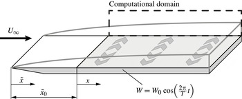
A graphical representation of the simulation set-up is given in figure 1. The computational domain starts at distance
 $\tilde{x}_{0}=33$
from the leading edge of the flat plate. This location defines the origin of the coordinate
 $x\equiv \tilde{x}-\tilde{x}_{0}$
. Lengths are normalized by the inlet 99 % boundary-layer thickness,
 ${\it\delta}_{0}$
, and velocities are normalized by the free-stream value,
 $U_{\infty }$
. The inlet Reynolds number based on
 ${\it\delta}_{0}$
is
 $\mathit{Re}_{{\it\delta}_{0}}=800$
(in terms of the Blasius length scale,
 $\mathscr{L}=\sqrt{\tilde{x}{\it\nu}/U_{\infty }}$
, the inlet Reynolds number is
 $\mathit{Re}_{\mathscr{L}_{0}}=162$
). In order to relate to the literature on fully turbulent flows, dimensionless wall distances
 $y^{+}=yu_{{\it\tau}}/{\it\nu}$
, forcing periods
 $T^{+}=Tu_{{\it\tau}}^{2}/{\it\nu}$
and velocities
 $W^{+}=W_{0}/u_{{\it\tau}}$
are supplied where beneficial. The friction velocity,
 $u_{{\it\tau}}$
, is extracted at the onset of the fully turbulent flow regime in the respective cases.
Schematic of the computational domain.

The length, width and height of the computational domain are 1200, 30 and 40, respectively, and the number of grid points in these dimensions are 4096, 192 and 192. The grid resolution is thus slightly finer than that adopted by Jacobs & Durbin (Reference Jacobs and Durbin2001), who performed an extensive grid refinement study. The grid spacing in the streamwise (
 $x$
) and spanwise (
 $z$
) dimensions is uniform. Grid stretching using a hyperbolic tangent function is used in the wall-normal coordinate (
 $y$
) to ensure a fine grid resolution near the wall. Throughout the streamwise extent of the computational domain, the coarsest grid resolution at the wall in terms of viscous units is
 ${\rm\Delta}y_{wall}^{+}=0.38$
. The streamwise and spanwise grid spacings are
 ${\rm\Delta}x^{+}=5.56$
and
 ${\rm\Delta}z^{+}=2.95$
, respectively.
The top boundary condition balances the growth of the boundary layer by a positive wall-normal velocity in order to ensure a zero mean pressure gradient in the streamwise direction. Homogeneous Neumann conditions are applied for the streamwise and spanwise velocity components at that boundary. A convective outflow condition is used at the exit of the domain, and periodicity is enforced in the spanwise direction. No-slip conditions are prescribed at the bottom wall. In addition, spanwise wall oscillation is applied over the full extent of the computational domain,
 $$\begin{eqnarray}W(y=0,t)=W_{0}\cos \left(\frac{2{\rm\pi}}{T}t\right).\end{eqnarray}$$
The transverse forcing starts at the inlet of the computational domain, and causes the development of a Stokes boundary layer. It can be shown that, in the limit of large downstream distances, the spanwise velocity field approaches the analytical solution to the Stokes second problem,
 $$\begin{eqnarray}W_{Stokes}(y,t)=W_{0}\exp \left(-\sqrt{\frac{{\rm\pi}}{{\it\nu}T}}\,y\right)\cos \left(\frac{2{\rm\pi}}{T}t-\sqrt{\frac{{\rm\pi}}{{\it\nu}T}}\,y\right).\end{eqnarray}$$
With increasing
 $x$
, the thickness of the Stokes layer in the DNS,
 ${\it\delta}_{w}$
, becomes proportional to
 $\sqrt{2{\rm\pi}T/{\it\nu}}$
. The boundary-layer thickness,
 ${\it\delta}$
, on the other hand, grows with downstream distance. Therefore, beyond a small region near the inlet, the ratio
 ${\it\delta}_{w}/{\it\delta}$
decays monotonically.
The time-harmonic forcing introduces a periodic component into the flow field. Hence a triple decomposition of flow variables is adopted, 
where
 ${\bar{a}}$
denotes the spanwise and time average,
 ${\tilde{a}}_{{\it\varphi}}$
is the periodic component and
 $a^{\prime }$
is the stochastic fluctuation. The quantity
 $\langle a\rangle _{{\it\varphi}}$
is the average at a particular phase,
 ${\it\varphi}(t)=(1/T)\,\text{mod}(t,T)$
, and comprises the time-averaged mean and the periodic component. The quantity
 $a^{\prime \prime }$
is the sum of the periodic component and the stochastic fluctuation.
For finite distances to the leading edge, the phase-averaged velocity profile
 $\tilde{w}(y,t)$
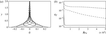
obtained from DNS differs from the analytical Stokes layer profile (2.2). This difference is presented in figure 2(a), and is quantified using the integral measure,
 $$\begin{eqnarray}q_{T}(x)=\frac{1}{T{\it\delta}_{w}}\int _{0}^{T}\int _{0}^{\infty }\frac{\Vert \tilde{w}-W_{Stokes}\Vert }{W_{0}}\text{d}y\text{d}t.\end{eqnarray}$$
The deviation of
 $\tilde{w}$
from the Stokes profile increases for longer oscillation periods, but remains at least two orders of magnitude smaller than
 $\tilde{w}$
.
(a) Wall-normal profiles of
 $\tilde{w}(y,t)$
(solid) and
 $W_{Stokes}$
(dashed) for
 $T=200$
. Eight equidistant phases are shown at
 $x=200$
. (b) Measure
 $q_{T}$
for the deviation between
 $\tilde{w}(y,t)$
and
 $W_{Stokes}$
as a function of downstream distance for
 $T=10$
(solid),
 $T=200$
(dashed) and
 $T=800$
(dash-dotted).

In order to initiate bypass transition in the simulations, the Blasius profile at the inlet to the computational domain is supplemented with a moderate level of free-stream turbulence with intensity
 $Tu_{FS}=3\,\%$
. Following Jacobs & Durbin (Reference Jacobs and Durbin2001), the inlet perturbations can be expressed as a weighted superposition of eigenfunctions of the continuous spectra of the homogeneous Orr–Sommerfeld and Squire operators. This approach inherently avoids the free-stream bias towards the streamwise component in the coupled Orr–Sommerfeld/Squire problem, which was recently pointed out by Dong & Wu (Reference Dong and Wu2013). Downstream of the inflow plane, the evolution of the flow is computed by direct simulations and therefore takes into account non-parallel and nonlinear effects. The methodology has been adopted successfully in a number of earlier studies (e.g. Brandt et al.
Reference Brandt, Schlatter and Henningson2004; Schrader, Brandt & Henningson Reference Schrader, Brandt and Henningson2009; Schrader, Subir & Brandt Reference Schrader, Subir and Brandt2010). It faithfully reproduces the mechanics of bypass transition as demonstrated by a number of comparisons with experiments. For example, Brandt et al. (Reference Brandt, Schlatter and Henningson2004) and more recently Nolan & Zaki (Reference Nolan and Zaki2013) showed that the streamwise energy amplification and the downstream development of the shape factor agree with the results by Matsubara & Alfredsson (Reference Matsubara and Alfredsson2001). The measurements by Mandal, Venkatakrishnan & Dey (Reference Mandal, Venkatakrishnan and Dey2010) showed good agreement between the properties of their streaks and those observed by Jacobs & Durbin (Reference Jacobs and Durbin2001). Matsubara & Alfredsson (Reference Matsubara and Alfredsson2001) concluded that their results ‘provide an experimental verification of the simulated picture’.
The simulation set-up adopted herein excludes the leading-edge region. In two earlier studies, Nagarajan, Lele & Ferziger (Reference Nagarajan, Lele and Ferziger2007) and later Ovchinnikov, Choudhari & Piomelli (Reference Ovchinnikov, Choudhari and Piomelli2008) performed simulations of the entire plate including the leading edge. Their results showed that, when the leading edge is blunt or the free-stream turbulence intensity is relatively high, leading-edge receptivity can become important and should be taken into account. Their simulations also affirmed, however, that the approach adopted herein accurately captures the bypass transition mechanism that is active in the case of a slender leading edge.
The amplitudes of the individual inlet perturbations are assigned such that a von Kármán spectrum is obtained in the free stream,
 $$\begin{eqnarray}E({\it\kappa})=Tu_{FS}^{2}\frac{L^{5}{\it\kappa}^{4}}{C(1+({\it\kappa}L)^{2})^{17/6}},\end{eqnarray}$$
where
 $Tu_{FS}$
is the free-stream turbulence intensity, and
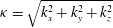 ${\it\kappa}=\sqrt{k_{x}^{2}+k_{y}^{2}+k_{z}^{2}}$
is the magnitude of the wavenumber vector. The length scale
 $L$
is related to the integral scale
 $L_{11}=(1/Tu_{FS})\int _{0}^{\infty }\overline{u^{\prime }(x)u^{\prime }(x+r)}\text{d}r$
by
 $L=(55C/9{\rm\pi})L_{11}$
. A choice of
 $C=0.688$
leads to a peak of the energy spectrum at unit wavelength. The most energetic perturbations thus have wavelengths of the order of the boundary-layer thickness.
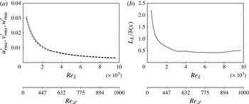
The downstream evolution of the perturbation field in the free stream is given in figure 3 for a reference simulation in the absence of wall oscillation. A nearly isotropic decay of the root mean square (r.m.s.) velocity fluctuations, which follows the power law
 $Tu_{FS}\sim \tilde{x}^{-0.69}$
, is captured in figure 3(a). Figure 3(b) shows the integral length scale
 $$\begin{eqnarray}L_{k}=\frac{k^{3/2}}{{\it\varepsilon}},\end{eqnarray}$$
where
 $k$
is the turbulence kinetic energy and
 ${\it\varepsilon}$
is the rate of energy dissipation, evaluated in the free stream and normalized by the local boundary-layer thickness. After an initial decay, the normalized length scale remains virtually constant over the remainder of the computational domain. A similar trend was observed in the experimental study by Kurian & Fransson (Reference Kurian and Fransson2009).
Free-stream decay of turbulence: (a) r.m.s. of the velocity fluctuations
 $u^{\prime }$
(dashed),
 $v^{\prime }$
(dash-dotted),
 $w^{\prime }$
(dash-double dotted) versus Reynolds number. (b) Turbulent length scale
 $L_{k}$
normalized by the local boundary-layer thickness
 ${\it\delta}$
versus Reynolds number.

3. Integral performance measures
This section provides an overview of the effect of the wall oscillation on the transition process. Selected results obtained from the DNS are presented, and focus is placed on statistical measures that demonstrate the potential of the forcing to delay bypass breakdown.
The skin friction coefficient
 $$\begin{eqnarray}C_{f}=\frac{\displaystyle {\it\mu}\frac{\partial U}{\partial y}|_{y=0}}{{\textstyle \frac{1}{2}}{\it\rho}U_{\infty }^{2}}\end{eqnarray}$$
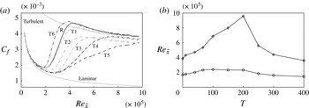
along the flat plate is reported in figure 4(a) for a range of forcing periods and a constant forcing amplitude,
 $W_{0}=0.25$
. In agreement with the direct simulations by Jacobs & Durbin (Reference Jacobs and Durbin2001), and the experimental studies of Roach & Brierley (Reference Roach and Brierley1990), the maximum
 $C_{f}$
at transition onset overshoots the turbulence correlation,
 $C_{f,\,turbulent}=0.455\ln ^{-2}(0.06\,\mathit{Re}_{\tilde{x}})$
(White Reference White2005). The downstream locations of the onset and completion of transition for all cases are identified by the first local minimum and the subsequent local maximum of the
 $C_{f}$
curve, respectively. The corresponding Reynolds numbers,
 $\mathit{Re}_{\tilde{x},s}$
and
 $\mathit{Re}_{\tilde{x},e}$
, are plotted in figure 4(b) versus the forcing period. For the reference case without forcing (given by
 $T=0$
), the transition process spans the Reynolds-number range
 $2\times 10^{5}\leqslant \mathit{Re}_{\tilde{x}}\leqslant 3.8\times 10^{5}$
, or
 $350\leqslant \mathit{Re}_{{\it\theta}}\leqslant 650$
, where
 ${\it\theta}$
is the momentum thickness.
(a) Skin friction coefficient. Reference simulation (R, solid) and forcing with amplitude
 $W=0.25$
and periods
 $T=10$
(T1, grey dash-dotted),
 $T=40$
(T2, grey dashed),
 $T=67$
(T3, grey dash-double dotted),
 $T=100$
(T4, black dash-dotted),
 $T=200$
(T5, black dashed) and
 $T=400$
(T6, black dash-double dotted). (b) Reynolds number at the onset (
 $\mathit{Re}_{\tilde{x},s}$
, circles) and completion (
 $\mathit{Re}_{\tilde{x},e}$
, diamonds) of transition.

The effect of the forcing on transition depends on the period of the spanwise flow. For the shortest period,
 $T=10$
, only a marginal deviation from the unforced reference case is observed, with transition completed at
 $\mathit{Re}_{\tilde{x}}\approx 4.3\times 10^{5}$
. In this context, it should be noted that the thickness of the Stokes layer scales as
 ${\it\delta}_{w}\sim \sqrt{T}$
. Hence, for very short forcing periods,
 ${\it\delta}_{w}$
is small compared to the Blasius boundary-layer thickness,
 ${\it\delta}_{w}/{\it\delta}\ll 1$
. In these cases, the spanwise flow is primarily limited to a region very close to the wall. For longer forcing periods, the thickness of the Stokes layer becomes larger, and has a more substantial influence on the transition process.
Forcing with periods
 $T\in [40,250]$
generally has two effects. The location of transition onset is shifted downstream. In addition, the transition region is extended in the streamwise direction. For the particular case
 $T=200$
, the flow is still intermittently laminar at the end of the simulation domain, which corresponds to
 $\mathit{Re}_{\tilde{x}}=9.86\times 10^{5}$
. The remainder of this work focuses primarily on this particular case of ‘optimal’ forcing.
Any further increase of the forcing period beyond the optimal value quickly diminishes the delay in transition. The oscillation period
 $T=300$
yields virtually identical values for transition onset and completion as the reference simulation. For
 $T=400$
, laminar–turbulent breakdown is accelerated and fully turbulent flow is established farther upstream than in the absence of spanwise forcing.
A wealth of earlier studies investigated the potential of spanwise wall oscillation to reduce drag in turbulent flows. The skin friction curves for the forcing periods of
 $T=40$
and
 $T=67$
reproduce this behaviour. After the completion of transition, the local wall shear in these cases remains between 10 and 12 % below the correlation for fully turbulent flow. In wall units, these forcing periods are
 $T^{+}=59$
and
 $T^{+}=99$
, and the present forcing amplitude
 $W_{0}=0.25U_{\infty }$
is equivalent to
 $W^{+}=5.81$
. Choi (Reference Choi2002) observed a reduction of drag in a turbulent boundary layer by approximately 45 % at
 $T^{+}=100$
and a higher amplitude
 $W^{+}=15$
. For the same forcing period and a slightly lower amplitude
 $W_{0}^{+}=12$
, Touber & Leschziner (Reference Touber and Leschziner2012) achieved a skin friction reduction by 38 % in fully turbulent channel flow. More recently, Lardeau & Leschziner (Reference Lardeau and Leschziner2013) found that the optimal forcing period of turbulent boundary layers is approximately
 $T^{+}=70$
.
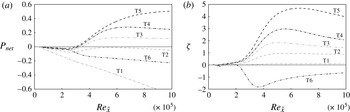
In order to determine whether transition delay yields an energetic advantage, the power requirement of the spanwise forcing,
 $\overline{P_{forcing}}$
, must be taken into account. The net energetic gain is
 $$\begin{eqnarray}\displaystyle \overline{P_{net}}(x)\! & = & \displaystyle \!\overline{P_{prop,\,ref}}(x)-\overline{P_{prop,\,forced}}(x)-\overline{P_{forcing}}(x)\nonumber\\ \displaystyle \! & = & \displaystyle \!{\rm\Delta}\overline{P_{prop}}-\overline{P_{forcing}},\end{eqnarray}$$
where
 $\overline{P_{prop,\,ref}}$
and
 $\overline{P_{prop,\,forced}}$
are the propulsion powers in the reference and forced cases. Results for
 $\overline{P_{net}}$
are provided in figure 5(a) for a range of forcing periods. Very short periods (
 $T=10$
) show the most negative energetic balance. This outcome is due to a negligible reduction of overall drag, combined with a relatively high power requirement, since
 $\overline{P_{forcing}}\sim 1/\sqrt{T}$
. When the forcing period is increased, transition delay and a continuously decreasing power requirement of the forcing lead to an optimum
 $\overline{P_{net}}$
at
 $T=200$
. Beyond this forcing period, there is a sharp increase in overall drag and thus
 $\overline{P_{prop}}$
, which outweighs the further decrease in the forcing power requirement. For
 $T=400$
, the acceleration of the breakdown process causes
 ${\rm\Delta}\overline{P_{prop}}$
to become negative.
(a) Net savings. (b) Relative performance. Forcing with amplitude
 $W=0.25$
and periods
 $T=10$
(T1, grey dash-dotted),
 $T=40$
(T2, grey dashed),
 $T=67$
(T3, grey dash-double dotted),
 $T=100$
(T4, black dash-dotted),
 $T=200$
(T5, black dashed) and
 $T=400$
(T6, black dash-double dotted).

The relative energetic performance,
 $$\begin{eqnarray}{\it\zeta}=\frac{{\rm\Delta}\overline{P_{prop}}(x)}{\overline{P_{forcing}}(x)},\end{eqnarray}$$
normalizes the power savings by the power input into the spanwise forcing. Figure 5(b) presents
 ${\it\zeta}$
for a range of forcing periods and shows that the energetic savings at the optimal forcing period outweigh the power requirement of the transverse forcing by a factor of four.
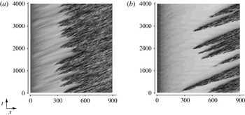
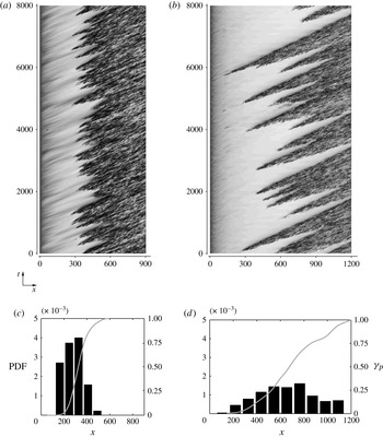
The statistical results presented so far clearly demonstrate the ability of the wall forcing to reduce viscous drag, and motivate an examination of the underlying behaviour of the flow. A concise overview of the influence of the forcing on the transition process is provided by the space–time diagrams in figure 6. The contours represent the level of the streamwise velocity at a particular spanwise position for a long span of time. Dark regions correspond to fully turbulent flow. Each of the ‘wedges’ pointing upstream represents the formation of a single turbulent spot. It is seen that, in the presence of the forcing, the frequency of occurrence of breakdown events is markedly reduced.
Space–time diagrams of the streamwise velocity,
 $u$
, recorded at
 $y/{\it\delta}(x)=0.40$
. (a) Unforced reference case. (b) Optimal forcing.

In the subsequent sections, the cause of the change in transition location and the frequency of spot inception are examined. The influence of the optimal wall forcing on boundary-layer streaks is discussed, followed by a study of the secondary instability of the base flow.
4. Effect of optimal forcing on the pre-transitional boundary layer
Laminar boundary-layer streaks are a central element in bypass transition. Even though they are dominated by the streamwise velocity component, the streaks amplify due to a displacement of the mean momentum by relatively weaker wall-normal perturbations. This section presents a comprehensive analysis of the influence of the spanwise forcing on the streaks themselves, as well as on the lift-up mechanism that causes them.
4.1. Boundary-layer streaks
In the pre-transitional boundary layer, the streamwise stochastic fluctuations,
 $u^{\prime }$
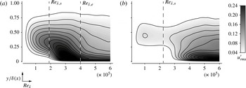
, provide a suitable starting point to examine the influence of the forcing on the streaks. Contours of the r.m.s. of
 $u^{\prime }$
are provided in figure 7. The reference case shows continuous growth of the fluctuation amplitude upstream of
 $\mathit{Re}_{\tilde{x},s}$
, with the maximum located at
 $y/{\it\delta}(x)\approx 0.4$
. This compares favourably with the experimental studies by Matsubara & Alfredsson (Reference Matsubara and Alfredsson2001), who located the peak of the streamwise velocity fluctuation at 1.3 times the local displacement thickness, or equivalently
 $y/{\it\delta}(x)\approx 0.45$
. A local peak is reached at the centre of the transition zone,
 $\mathit{Re}_{\tilde{x}}\approx 3\times 10^{5}$
. Once the flow has become fully turbulent, the position of the maximum
 $u_{rms}^{\prime }$
moves closer to the wall and is located at approximately 5 % of the local boundary-layer thickness. In the presence of the forcing (figure 7
b), initial streak growth remains below the levels observed for the reference case. The results suggest that the amplification of streaks is delayed to larger
 $\mathit{Re}_{\tilde{x}}$
.
R.m.s. of the streamwise stochastic velocity fluctuations,
 $0.04\leqslant u_{rms}^{\prime }\leqslant 0.24$
. (a) Reference simulation. (b) Optimal forcing.

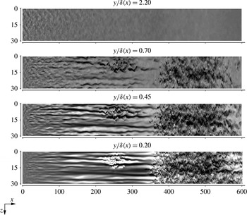
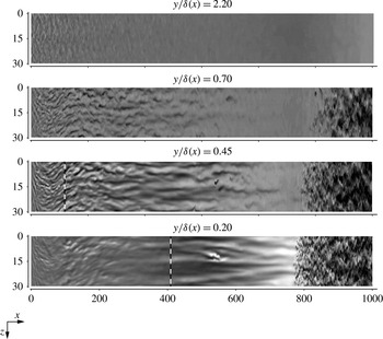
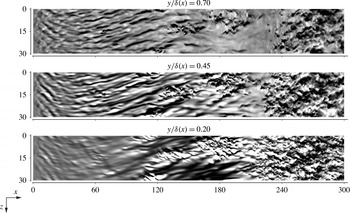
The effect of the spanwise oscillatory flow on the streaks is also apparent in instantaneous flow fields. For the purpose of comparison, figures 8 and 9 show contours of
 $u^{\prime }$
from the reference and the optimal forcing simulations. The plane views are at constant
 $y/{\it\delta}(x)$
, and thus follow the growth of the boundary layer. The top panel shows the free stream, where the perturbations decay as they are convected downstream in both cases. The three remaining panels are within the boundary layer.
Top views, unforced reference simulation. Contours of the stochastic fluctuation of the streamwise velocity component
 $-0.20\leqslant u^{\prime }\leqslant 0.20$
.

Top views, optimal forcing. Contours of the stochastic fluctuation of the streamwise velocity component,
 $-0.20\leqslant u^{\prime }\leqslant 0.20$
. The dashed vertical line gives the location where the plane crosses the spanwise Stokes layer.

Since they are generated by lift-up, the streaks close to the edge of the boundary layer are generally slower than the surrounding fluid,
 $u^{\prime }<0$
. On the other hand, near-wall streaks (
 $y/{\it\delta}(x)=0.20$
) are characterized by a velocity surplus relative to the mean flow,
 $u^{\prime }>0$
. Inside the boundary layer, the formation of streaks is significantly weakened by the spanwise oscillatory flow (figure 9). The influence of the forcing is most apparent at
 $y/{\it\delta}(x)=0.20$
, where
 $\tilde{w}$
is highest among the shown planes. The flow field in that view is free from Klebanoff streaks upstream of
 $x\approx 350$
. Relative to figure 8, the flow fields under the influence of the forcing clearly indicate an absence of energetic streaky structures in the boundary layer. Isolated streamwise-elongated features are observed, which are nonetheless shorter in extent than those in the reference case. The flow remains laminar, without any localized breakdown events, until a sudden change to fully turbulent flow near
 $x\approx 800$
(
 $\mathit{Re}_{\tilde{x}}=6.67\times 10^{5}$
).
In order to examine the spectral content of the fluctuation field, the energy frequency spectrum is evaluated,
 $$\begin{eqnarray}{\hat{E}}_{u}(F)=\left(\int _{-\infty }^{\infty }u^{\prime }(t)\exp (-2{\rm\pi}\text{i}Ft)\text{d}t\right)^{2}\!,\end{eqnarray}$$
where
 $F=10^{6}{\it\omega}{\it\nu}/U_{\infty }^{2}$
is the non-dimensional frequency. It should be noted that the lowest frequency at the inflow is
 $F=480$
, which is relatively high in comparison to that of the streaks. As demonstrated in earlier works, nonlinear interactions lead to the rapid broadening of the spectrum and the maximum shifts towards the low-frequency streamwise-elongated streaks (Jacobs & Durbin Reference Jacobs and Durbin2001; Brandt et al.
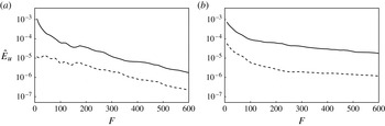
Reference Brandt, Schlatter and Henningson2004). The spectrum for the reference and forced cases at the downstream position
 $x=170$
(
 $\mathit{Re}_{\tilde{x}}=1.62\times 10^{5}$
), which is located upstream of spot inception, is given in figure 10. At this location, the local thickness of the spanwise Stokes layer is
 ${\it\delta}_{w}(x)/{\it\delta}(x)=0.32$
. The energy of the streamwise velocity component is primarily in the low-frequency range and decreases logarithmically with increasing frequency for both the reference and unforced cases. The presence of the forcing nonetheless reduces the energy contained in low-frequency perturbations by more than an order of magnitude. This finding affirms that the decrease in
 $u_{rms}^{\prime }$
can be attributed to the weakening of the streaks in the presence of spanwise wall oscillation.
Temporal energy spectra of the streamwise velocity fluctuation
 $u^{\prime }$
, evaluated at
 $y/{\it\delta}(x)=0.4$
: (a)
 $x=170$
; (b)
 $x=400$
. Reference simulation (solid) and optimal forcing (dashed).

Farther downstream, at
 $x=400$
, the flow in the reference simulation has become intermittent, and an increase of the energy in high-frequency perturbations is recorded in the spectra. A similar trend is observed for the forced case, although, in absolute terms, the energy level remains substantially below the reference case for all
 $F$
. At this downstream position, the local thickness of the spanwise Stokes layer is
 ${\it\delta}_{w}(x)/{\it\delta}(x)=0.21$
.
The spectral make-up of the disturbance field in terms of the spanwise perturbation wavenumber,
 $k_{z}$
, is evaluated as
 $$\begin{eqnarray}E_{u}(k_{z},F)=\left(\int _{-\infty }^{\infty }\int _{-\infty }^{\infty }u^{\prime }(z,t)\exp (-\text{i}2{\rm\pi}(Ft+k_{z}z))\text{d}t\text{d}z\right)^{2}.\end{eqnarray}$$
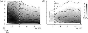
Results for the reference and optimally forced cases are compared in figure 11. The spectra show small energy content at low Reynolds number owing to the absence of low-frequency disturbances at the inlet. Downstream of that region, the reference simulation develops highly energetic perturbations, with a peak at spanwise wavenumber
 $k_{z}\approx 1.4$
. The corresponding spanwise wavelength is approximately twice the local boundary-layer thicknesses, which is representative of the pre-transitional streaks. Transition to turbulence downstream of
 $\mathit{Re}_{\tilde{x}}\approx 2\times 10^{5}$
is characterized by a redistribution of energy, which causes
 $E_{u}(k_{z},F=16)$
to decay. In the presence of the wall motion, the initial amplification of low-frequency perturbations is substantially reduced. The level of
 $E_{u}$
remains below that of the reference case throughout the investigated range of Reynolds numbers.
Logarithm of the spanwise energy spectra of
 $u^{\prime }$
versus downstream Reynolds number at
 $y/{\it\delta}(x)=0.40$
. (a) Reference simulation. (b) Optimal forcing. The contours span the range
 $-8\leqslant \log E_{u}\leqslant 8$
, for
 $F=16$
.

4.2. Lift-up mechanism
In order to examine the mechanism for the weakening of the streaks, the budget of the kinetic energy in the streamwise velocity fluctuation,
 $k^{u}=\frac{1}{2}\overline{u^{\prime }u^{\prime }}$
, is considered,
 $$\begin{eqnarray}\underbrace{\overline{u_{l}}\frac{\partial }{\partial x_{l}}k^{u}}_{C^{u}}\underbrace{+\,\overline{u^{\prime }u_{l}^{\prime }}\frac{\partial }{\partial x_{l}}\overline{u}}_{P^{u}}=\underbrace{-\frac{1}{{\it\rho}}\frac{\partial }{\partial x}\overline{u^{\prime }p^{\prime }}}_{R^{u}}\underbrace{-\,{\it\nu}\overline{\frac{\partial }{\partial x_{l}}u^{\prime }\frac{\partial }{\partial x_{l}}u^{\prime }}}_{D^{u}}\underbrace{-\,\frac{1}{2}\frac{\partial }{\partial x_{l}}\overline{u_{l}^{\prime }u^{\prime }u^{\prime }}}_{T^{u}}+{\it\nu}\frac{\partial ^{2}}{\partial x_{l}\partial x_{l}}k^{u}.\end{eqnarray}$$
The terms in this equation describe the advection (
 $C^{u}$
), production (
 $P^{u}$
), pressure redistribution (
 $R^{u}$
), dissipation (
 $D^{u}$
) and turbulent transport (
 $T^{u}$
) of disturbance kinetic energy. Since
 $k^{u}$
is dominated by the streaks, the production term,
 $P^{u}$
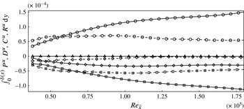
, is directly related to amplification of streaks via the lift-up process. The boundary layer integrals of the production, dissipation, convection and pressure reduction terms of
 $k^{u}$
for both the reference and optimally forced cases are presented in figure 12. A significant reduction in
 $P^{u}$
is observed in the presence of the wall motion, where the streaks are also weaker. Outside a small region near the inflow, the dissipation of kinetic energy is also significantly lower in the forced case.
Budget of the kinetic energy in streamwise stochastic fluctuations, integrated over the local thickness of the boundary layer. Production (
 $P^{u}$
, circles), dissipation (
 $D^{u}$
, squares), convection (
 $C^{u}$
, diamonds) and pressure redistribution (
 $R^{u}$
, triangles). Reference (solid) and forced (dashed) cases.

In order to further assess the influence of the wall forcing on the lift-up mechanism, the joint probability density function (PDF) of
 $u^{\prime }$
and
 $v^{\prime }$
, or
 $G(u^{\prime },v^{\prime })$
, is evaluated. The probability
 $P$
for a pair of values
 $(u^{\prime },v^{\prime })$
to lie within the interval
 $[u_{1}^{\prime },u_{2}^{\prime }]\times [v_{1}^{\prime },v_{2}^{\prime }]$
is obtained by integrating
 $G(u^{\prime },v^{\prime })$
,
 $$\begin{eqnarray}P([u_{1}^{\prime },u_{2}^{\prime }]\times [v_{1}^{\prime },v_{2}^{\prime }])=\int _{v_{1}^{\prime }}^{v_{2}^{\prime }}\int _{u_{1}^{\prime }}^{u_{2}^{\prime }}G(u^{\prime },v^{\prime })\text{d}u^{\prime }\text{d}v^{\prime }.\end{eqnarray}$$
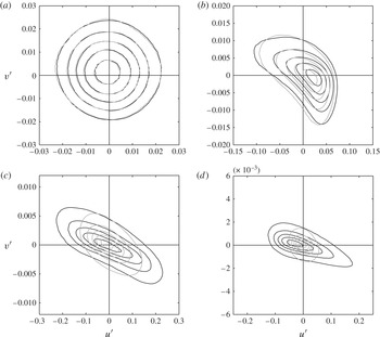
The free-stream behaviour of the fluctuation field at the wall distance
 $y/{\it\delta}(x)=1.6$
is given in figure 13(a). The circular contours reflect the isotropy of the free-stream perturbation field. Inside the boundary layer, the shape of the contour lines is stretched in the
 $u^{\prime }$
direction and compressed in the
 $v^{\prime }$
direction. The reduced extent of the joint PDFs with respect to
 $v^{\prime }$
can be attributed to the combined effects of shear sheltering and wall blocking. The formation of Klebanoff streaks within the boundary layer causes the expansion of the joint PDFs in the direction of
 $u^{\prime }$
. In the reference case, the joint PDFs become increasingly biased towards quadrants II (ejections:
 $u^{\prime }<0,\ v^{\prime }>0$
) and IV (sweeps:
 $u^{\prime }>0,\ v^{\prime }<0$
) inside the boundary layer. Both sweeps and ejections are markedly weakened in the presence of the forcing. This effect is most noticeable close to the wall, where the magnitude of the spanwise base flow is highest.
Joint PDFs for the streamwise and wall-normal velocity fluctuations at
 $x=170$
: (a)
 $y/{\it\delta}(x)=1.6$
; (b)
 $y/{\it\delta}(x)=0.8$
; (c)
 $y/{\it\delta}=0.4$
; (d)
 $y/{\it\delta}=0.2$
(located inside the spanwise Stokes layer). Contours give lines of 10, 30, 50, 70 and 90 % probability for the reference simulation (black) and optimal forcing (grey).

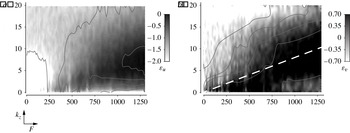
In order to examine whether there exists a preferential orientation in spectral space for energy amplification, the quantity
 $$\begin{eqnarray}{\it\varepsilon}_{u}=\int _{0}^{{\it\delta}(x)}\log E_{u,\,forced}-\log E_{u,\,ref}\text{d}y\end{eqnarray}$$
is considered. Here,
 $E$
is the kinetic energy as a function of
 $F$
and
 $k_{z}$
. The results for the streamwise and wall-normal fluctuations, respectively, are shown in figure 14(a,b). When considering
 $u^{\prime }$
, it should be emphasized that
 ${\it\varepsilon}_{u}$
is negative for all
 $F$
and
 $k_{z}$
. The difference is most pronounced in the region
 $F<200$
,
 $k_{z}<10$
, which is associated with boundary-layer streaks.
Difference between the energy of reference and optimally forced cases at
 $x=65$
, integrated over the extent of the boundary layer. (a) Streamwise component
 $-2\leqslant {\it\varepsilon}_{u}\leqslant 0$
. (b) Wall-normal component
 $-0.7\leqslant {\it\varepsilon}_{v}\leqslant 0.7$
.

The difference in the spectra of
 $v^{\prime }$
, on the other hand, contains regions of both positive and negative
 ${\it\varepsilon}_{v}$
. The energy in the forced case is highest along rays starting at the origin, and pointing towards
 $F=1300$
,
 $k_{z}=10$
, marked by the dashed line in figure 14(b). The non-dimensional frequency is related to the streamwise wavenumber of the perturbations via
 $k_{x}=FU_{\infty }^{2}/(10^{6}c{\it\nu})$
, where
 $c$
is the phase speed of the disturbance. Assuming
 $c\in [0.4,0.85]$
, the angle of these rays ranges from 14 to 6°. This angle has been explained using a model problem and comparing the diffusive and convective time scales of free-stream perturbations (Hack & Zaki Reference Hack and Zaki2012). Owing to the wall forcing, the base flow is three-dimensional. Disturbances whose wavenumber vector is perpendicular to the shear vector can preferentially diffuse into the boundary layer.
4.3. Streak amplitudes
The discussion of the amplitude of boundary-layer streaks has thus far relied on statistical measures of
 $u^{\prime }$
. For example, it was shown that the r.m.s. of
 $u^{\prime }$
decreases under the influence of the spanwise wall forcing. These results do not, however, differentiate the part of
 $u^{\prime }$
that indeed forms the streaks from the surrounding perturbations, since the entire disturbance field is sampled indiscriminately. In order to identify particular streaks, the methodology described by Nolan & Zaki (Reference Nolan and Zaki2013) is applied to time series that comprise 4000 snapshots from each of the reference and the optimally forced cases.
First, laminar flow regions are isolated using a laminar–turbulent discrimination technique. The local extrema of
 $u^{\prime }$
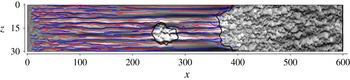
are subsequently identified in cross-flow planes, and streaks are reconstructed by connecting the extrema across adjacent planes. Using this approach, the streaks can be identified (see figure 15) and traced in space–time as Lagrangian objects. The spatial coordinates of streak
 $s$
are given by
 $\boldsymbol{x}^{s}(t)$
, and its amplitude is
 $\mathscr{A}_{u}^{s}(\boldsymbol{x}^{s},t)\equiv u^{\prime }(\boldsymbol{x}=\boldsymbol{x}^{s},t)$
.
High-speed (red) and low-speed (blue) streaks are identified in a flow field from the reference simulation. Black lines demarcate regions of turbulence. The background contours represent the streamwise velocity fluctuations,
 $-0.30\leqslant u^{\prime }\leqslant 0.30$
.

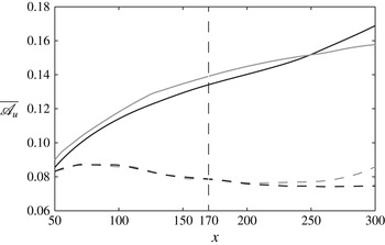
The average of the amplitudes of all streaks,
 $\overline{\mathscr{A}_{u}}=(1/S)\sum _{s}\mathscr{A}_{u}^{s}$
, is shown in figure 16 as a function of the downstream coordinate. Generally, the amplitudes of high-speed and low-speed streaks are approximately equal, in both the reference and forced cases. For the former, an increase in the amplitude with
 $x$
is observed, and
 $\overline{\mathscr{A}_{u}}$
grows from 0.09 at
 $x=50$
to 0.16 at
 $x=300$
. In the presence of the spanwise flow, the averaged amplitudes are significantly lower, and the relative difference to the reference simulation grows with downstream distance. At
 $x=300$
, the forcing has caused a reduction in the streak amplitude by a factor of two.
Amplitudes of high-speed (black) and low-speed (grey) streaks for reference (solid) and optimally forced (dashed) cases versus downstream position.

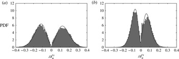
The PDFs of
 $\mathscr{A}_{u}^{s}$
for both the reference and forced cases at
 $x=170$
are presented in figure 17. Solid lines mark a fit for a type I general extreme value distribution. Inspection of the reference simulation shows that the peak of the PDF is located at approximately 15 % of the free-stream velocity for both high- and low-speed streaks. The wall forcing, on the other hand, leads to substantially narrower PDFs, with amplitudes of the majority of the streaks below 10 % of the free-stream velocity. It also eliminates high-amplitude streaks,
 $\mathscr{A}_{u}^{s}>0.25$
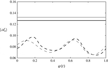
. Further analysis of the effect of the wall motion on the streaks is presented in figure 18, where the phase-averaged amplitude,
 $\langle \mathscr{A}_{u}\rangle$
, is plotted versus the phase of the base flow at
 $x=170$
. In the forced case, the streak amplitude oscillates twice per base-flow period between
 $\langle \mathscr{A}_{u}\rangle =0.07$
and 0.10. This frequency doubling is expected since the wall oscillation is symmetric in the positive and negative spanwise directions. Despite this preferential amplification at
 ${\it\varphi}\approx 0.15$
and
 ${\it\varphi}\approx 0.65$
, the streak amplitudes remain significantly weaker in the presence of the forcing relative to the reference simulation.
PDFs of the local streak amplitudes at
 $x=170$
. (a) Unforced reference case. (b) Optimal forcing.

Amplitudes of high-speed (black) and low-speed (grey) streaks for reference (solid) and optimally forced (dashed) cases versus the phase of the base flow at
 $x=170$
.

Boundary-layer streaks initiate breakdown to turbulence via the amplification of secondary instabilities. The recent study by Hack & Zaki (Reference Hack and Zaki2014) established a clear correlation between the amplitudes of streaks and the amplification rates of these instabilities. In that work, it was shown that the mean amplitude of the subset of streaks that cause breakdown to turbulence is approximately 30 % of the free-stream speed. This level of streak amplitude is nearly absent in the forced case. It is therefore expected that these streaks will be less likely to develop secondary instabilities – a point that is examined in detail in the next section.
5. Secondary instability and breakdown
The results presented so far have shown a substantial weakening of the boundary-layer streaks at the optimal wall oscillation. The low-frequency streaks themselves, however, do not immediately cause the formation of turbulent spots. Breakdown to turbulence is rather a consequence of high-frequency secondary instabilities of the streaky base state. The purpose of the present section is to relate the weaker boundary-layer streaks in the forced flow to the reduced frequency of turbulent-spot inception via the analysis of secondary instabilities.
5.1. Secondary instability analysis
The computational approach to investigate the secondary instability of the streaky boundary layer is based on the work of Blackburn & Sherwin (Reference Blackburn and Sherwin2004) and Barkley, Blackburn & Sherwin (Reference Barkley, Blackburn and Sherwin2008). The base flow of the stability analysis is given by instantaneous velocity profiles in the cross-flow plane that are extracted from DNS fields. The dependence of the base flow on
 $x$
and
 $t$
is therefore parametric. This approach is motivated by the weak time dependence of the streaky base state. For the present case with optimal forcing (
 $T=200$
), the time scale of the wall motion substantially exceeds that of the streak instabilities. The locally parallel base state of the instability analysis is
 $\boldsymbol{Q}_{stab}(y,z;x,t)=(U,V,W,P)_{stab}^{\text{T}}=(u(x,y,z,t)_{DNS},0,0,0)^{\text{T}}$
. The secondary instability is described by the state vector
 $\boldsymbol{q}_{2}(x,y,z,t)=(u,v,w,p)_{2}^{\text{T}}$
, which leads to the ansatz
 $\boldsymbol{q}=\boldsymbol{Q}_{stab}+\boldsymbol{q}_{2}$
for the perturbed base state.
A normal-mode assumption is adopted in
 $x$
,
 $$\begin{eqnarray}\boldsymbol{q}_{2}(x,y,z,t)=\hat{\boldsymbol{q}}_{2}(y,z,t)\exp (\text{i}{\it\alpha}x),\end{eqnarray}$$
where
 ${\it\alpha}$
is the streamwise instability wavenumber. The streak instability is assumed to be small in magnitude, so that quadratic terms may be neglected. The time evolution of
 $\boldsymbol{u}_{2}=(u,v,w)_{2}^{\text{T}}$
is hence described by the linear relation
 $$\begin{eqnarray}\frac{\partial }{\partial t}\hat{\boldsymbol{u}}_{2}=-\text{i}\unicode[STIX]{x1D647}\hat{\boldsymbol{u}}_{2},\end{eqnarray}$$
where
 $$\begin{eqnarray}\unicode[STIX]{x1D647}=\text{i}[(\unicode[STIX]{x1D644}-\boldsymbol{{\rm\nabla}}{\bf\Delta}^{-1}\boldsymbol{{\rm\nabla}}\boldsymbol{\cdot })(\boldsymbol{U}_{stab}\boldsymbol{\cdot }\boldsymbol{{\rm\nabla}})+(\boldsymbol{{\rm\nabla}}\boldsymbol{U}_{stab})\boldsymbol{\cdot }]+\frac{1}{Re}{\rm\nabla}^{2},\end{eqnarray}$$
and
 ${\bf\Delta}^{-1}$
is the formal inverse of the Laplacian. Integration of (5.2) gives
 $$\begin{eqnarray}\hat{\boldsymbol{u}}_{2}(t)=\unicode[STIX]{x1D63C}(t)\hat{\boldsymbol{u}}_{2}(0),\end{eqnarray}$$
with the fundamental solution operator
 $\unicode[STIX]{x1D63C}=\exp (-\text{i}\unicode[STIX]{x1D647}t)$
. The time dependence of an eigenfunction
 $\hat{\boldsymbol{u}}_{2}$
of
 $\unicode[STIX]{x1D647}$
with corresponding eigenvalue
 ${\it\sigma}$
is hence given by
 $\hat{\boldsymbol{u}}_{2}(t)=\hat{\boldsymbol{u}}_{2}(0)\exp (-\text{i}{\it\sigma}t)$
. The investigated base flow is exponentially stable if the imaginary part
 ${\it\sigma}_{i}$
of all eigenvalues is negative, and unstable otherwise. The numerical method for computing a subspectrum of
 $\unicode[STIX]{x1D647}$
is based on the IRAM scheme introduced by Sorensen (Reference Sorensen1992). The boundary conditions for the secondary instability at the wall and at the top of the computational domain are
 $$\begin{eqnarray}\displaystyle \displaystyle u_{2},v_{2},w_{2}=0 & \quad & \displaystyle \text{for }y=0,\end{eqnarray}$$
 $$\begin{eqnarray}\displaystyle \displaystyle v_{2},\frac{\partial u_{2}}{\partial y},\frac{\partial w_{2}}{\partial y}=0 & \quad & \displaystyle \text{for }y\rightarrow \infty .\end{eqnarray}$$
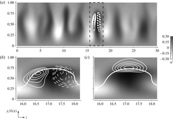
A visualization of a representative eigenfunction of a secondary streak instability is provided in figure 19. Background contours show the streamwise fluctuation field and lines indicate the eigenfunction of the most unstable secondary instability. The top panel shows the entire spanwise extent of the computational domain and demonstrates that the eigenfunction is localized around a single low-speed streak. The two lower panels provide enlarged views of the streamwise and spanwise components of the instability eigenfunction. In the case of the streamwise component, the eigenfunction is situated along the flanks of the streak and shows a spanwise antisymmetric configuration, such that
 $u_{2}$
is positive on the right-hand side and negative on the left-hand side of the streak. The eigenfunction of the spanwise component is situated on top of the streak and is spanwise symmetric with respect to the host streak. The combined effect of the two components is a sinusoidal deformation of the host streak, which grows in amplitude and eventually leads to the inception of a turbulent spot.
Eigenfunction of a streak instability (lines) and streamwise velocity fluctuation field
 $-0.30\leqslant u^{\prime }\leqslant 0.30$
(greyscale contours). (a) Entire spanwise extent of the domain with streamwise component of the eigenfunction. (b) Enlarged view with streamwise component of the eigenfunction. (c) Enlarged view with spanwise component of the eigenfunction. Dashed lines are negative values, and solid lines are positive values. The thick white line marks the critical layer.

In order to examine the impact of the wall forcing on the amplification of secondary instabilities, a statistical approach using a large number of stability analyses is pursued. The time interval between two consecutive analyses is
 ${\rm\Delta}t_{stab}=20$
. This time interval ensures that different phases of the oscillatory base flow are examined. A total of 200 time instances were investigated at the downstream position
 $x=170$
. It should be noted that the streamwise wavenumber
 ${\it\alpha}$
is an input parameter of the linear analysis. Therefore, at each time instance, six stability computations over the range
 ${\it\alpha}\in [0.3,1.3]$
were performed. This choice is motivated by earlier studies (Hack & Zaki Reference Hack and Zaki2014), which examined the range of
 ${\it\alpha}$
in detail. Only the maximum growth rate is included in the reported statistics. Furthermore, it should be pointed out that the instability analysis is purely temporal and thus differs from the DNS, which captures the spatio-temporal evolution of the instabilities. In a recent study, however, Hack & Zaki (Reference Hack and Zaki2014) have demonstrated that the temporal analysis can accurately capture the properties of the secondary instabilities of streaks.
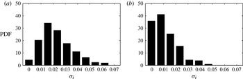
The results from the current stability analyses are presented in figure 20. The mean growth rate of the secondary instabilities halves from
 $\overline{{\it\sigma}_{i,\,ref}}=0.023$
in the reference case to
 $\overline{{\it\sigma}_{i,\,forced}}=0.011$
under the influence of the wall forcing. This reduction affects all growth rates in excess of 0.02. The work by Hack & Zaki (Reference Hack and Zaki2014) demonstrated that secondary instabilities with higher growth rates can be directly related to breakdown via turbulent spots. The current analysis thus explains the reduced frequency of occurrence of turbulent spots in the presence of the spanwise wall forcing, which was shown in the space–time diagram (figure 6).
PDFs of the growth rate
 ${\it\sigma}_{i}$
of the streak instabilities, evaluated at
 $x=170$
. (a) Unforced reference case. (b) Optimal forcing.

5.2. Formation of turbulent spots
For a closer study of the influence of the wall motion on the formation of turbulent spots, the space–time diagram from figure 6 is repeated in figure 21 for a longer time interval,
 $t\in [0,8000]$
. Comparison of the reference and forced cases substantiates the earlier observation of a lower rate of spot formation in the forced flow. In order to quantitatively corroborate the visual impression from the figure, the laminar–turbulent discrimination technique is employed, and the inception of turbulent spots is recorded. PDFs of the downstream position of spot inception are shown in the two lower panels of figure 21. It is seen that in the reference case practically all spots form upstream of
 $x\approx 400$
. In the presence of the forcing, the average location of spot formation is shifted downstream, with the peak of the distribution located at
 $x\approx 800$
.
(a,b) Space–time diagrams of the streamwise velocity,
 $u$
, at
 $y/{\it\delta}(x)=0.40$
. (c,d) PDFs of the location of spot inception. The grey line gives the local peak intermittency
 ${\it\gamma}_{p}$
. (a,c) Unforced reference case. (b,d) Optimal forcing.

The laminar–turbulent discrimination method may also be used to determine the fraction of time for which the flow at a given downstream location is turbulent. The indicator function
 ${\it\Gamma}(x,y,z,t)$
is set to unity if the flow is turbulent and to zero if the flow is laminar. Intermittency is then defined as the time and spanwise average of
 ${\it\Gamma}$
,
 $$\begin{eqnarray}{\it\gamma}(x,y)=\lim _{t^{\ast }\rightarrow \infty }\frac{1}{t^{\ast }L_{z}}\int _{t^{\ast }}\int _{L_{z}}{\it\Gamma}(x,y,z,t)\text{d}z\text{d}t,\end{eqnarray}$$
and the local peak intermittency is
 $$\begin{eqnarray}{\it\gamma}_{p}(x)=\max _{y}{\it\gamma}(x,y).\end{eqnarray}$$
Figure 21 shows that the flow in the reference simulation becomes fully turbulent at
 $x\approx 600$
(
 $\mathit{Re}_{\tilde{x}}=5.06\times 10^{5}$
). In the presence of the forcing, the flow approaches
 ${\it\gamma}_{p}=1$
at the downstream end of the computational domain, at
 $x=1200$
(
 $\mathit{Re}_{\tilde{x}}=9.86\times 10^{5}$
). The delay in breakdown to turbulence has been attributed to the weaker streaks in the pre-transitional flow and their reduced secondary instability.
6. Discussion
6.1. Variation of the forcing amplitude
The wall forcing is characterized by its period,
 $T$
, and its amplitude,
 $W_{0}$
. While the influence of
 $T$
was comprehensively examined in § 3, the forcing amplitude has so far been kept constant at
 $W_{0}=0.25$
. In order to provide a qualitative understanding of the influence of the forcing amplitude on the transition process, additional simulations were performed at various
 $W_{0}$
. For the two forcing periods
 $T=\{40,200\}$
, two additional amplitudes
 $W_{0}=0.10$
and
 $W_{0}=0.40$
were examined. All other parameters, including the turbulent inlet condition and the grid resolution, remained unchanged.
Further study of the period
 $T=40$
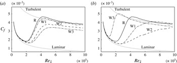
is motivated by the earlier reported reduction of skin friction in fully turbulent boundary layers at similar forcing periods (e.g. Lardeau & Leschziner Reference Lardeau and Leschziner2013). The skin friction coefficient is shown in figure 22(a). Both the onset and the completion of the transition process are increasingly shifted downstream with growing forcing amplitude. After the completion of transition, the local skin friction remains below the characteristic level of fully turbulent flow. This effect is more pronounced for higher forcing amplitudes, and thus qualitatively matches the results in various studies of viscous drag reduction in turbulent bounded shear flows.
Skin friction coefficient under variation of the forcing amplitude: (a)
 $T=40$
; (b)
 $T=200$
. Reference simulation (R, solid),
 $W_{0}=0.10$
(W1, dash-dotted),
 $W_{0}=0.25$
(W2, dashed) and
 $W_{0}=0.40$
(W3, dash-double dotted).

A second series of computations was performed for
 $T=200$
. This particular oscillation period was the optimal configuration with respect to transition delay and reduction in viscous drag at
 $W_{0}=0.25$
. The local skin friction coefficient is shown in figure 22(b), and demonstrates a strong dependence of the transition process on the amplitude of the forcing. For
 $W_{0}=0.10$
, the onset of transition is at the same downstream position as for
 $W_{0}=0.25$
, yet the streamwise extent of the transition region itself is substantially shortened. An increase in the forcing amplitude to
 $W_{0}=0.40$
sharply reverses the stabilizing effect of the forcing, and a very rapid breakdown to turbulence is observed, with transition starting upstream of the unforced case, at
 $x\approx 100$
. Fully turbulent flow is observed as early as
 $x\approx 300$
.
The fluctuation field in the case
 $T=200$
,
 $W_{0}=0.40$
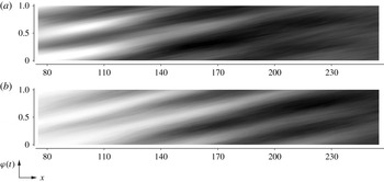
shows a clear phase dependence as demonstrated by the phase-averaged space–time diagrams provided in figure 23. Contours show the spanwise standard deviation of the fluctuation field,
 $$\begin{eqnarray}\langle u^{\prime }\rangle _{rms}=\left(\frac{1}{NL_{z}}\mathop{\sum }\limits_{N}\int _{0}^{L_{z}}u^{\prime \,2}\text{d}z\right)^{1/2},\end{eqnarray}$$
where
 $N=20$
is the number of sampled periods of the base flow. The periodicity is most prominent at the considered wall distance,
 $y/{\it\delta}(x)=0.30$
, which is slightly lower than the location of the peak
 $u^{\prime }$
associated with Klebanoff streaks.
Phase-averaged space–time diagrams: (a)
 $\langle u^{\prime }\rangle _{rms}$
; (b)
 $\langle v^{\prime }\rangle _{rms}$
. Forcing with
 $T=200$
,
 $W_{0}=0.40$
.

Results for the streamwise velocity component are shown in figure 23(a). A structure of alternating bands of high and low
 $\langle u^{\prime }\rangle _{rms}$
is observed with half the period of the base flow. In other words, each forcing period contains two intervals during which the fluctuations grow, separated by intervals in which the fluctuations decay again. The bands are aligned at an angle to the abscissa, which corresponds to a characteristic ‘speed’
 $c_{c}\approx 0.60$
with which the perturbation field travels downstream. As the flow becomes increasingly turbulent, the bands smear out and finally form a continuous region of high
 $\langle u^{\prime }\rangle _{rms}$
.
The standard deviation of the wall-normal velocity fluctuation,
 $v^{\prime }$
, shows a very similar behaviour (figure 23
b). While the magnitude of
 $\langle v^{\prime }\rangle _{rms}$
is initially lower than for the streamwise component, the observed angle of the bands is approximately identical. It is also clear that the phases of the streamwise and wall-normal fluctuations match, indicating a simultaneous amplification and decay of the two components.
Making use of the methodology introduced in § 5.2, spot formation in the case
 $T=200$
,
 $W_{0}=0.40$
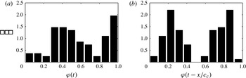
is investigated. Figure 24(a) shows a probability distribution for the formation of turbulent spots as a function of the phase of the base flow, irrespective of the downstream position at which breakdown occurs. Two mildly pronounced peaks are observed, which indicates that the frequency of breakdown to turbulence is the first harmonic of the base flow frequency. This phase dependence becomes more evident if the downstream position of the turbulent spots is incorporated to compute a corrected phase of spot inception using the phase speed
 $c_{c}=0.60$
. In figure 24(b), two well-defined maxima are seen, indicating a strong phase dependence of breakdown to turbulence in the case of high-amplitude forcing. Top views of the flow field for this case,
 $T=200$
and
 $W_{0}=0.40$
, are provided in figure 25. These visualizations indicate a generally high perturbation level inside the boundary layer. The perturbations are relatively short in the streamwise direction and hence clearly differ from typical boundary-layer streaks.
PDFs of the phase of spot inception. (a) Uncorrected phase,
 ${\it\varphi}(t)$
. (b) Corrected phase,
 ${\it\varphi}(t-x/c_{c})$
.

Top views, forcing with
 $T=200$
,
 $W_{0}=0.40$
. Fluctuation of the streamwise velocity component,
 $-0.10\leqslant u^{\prime }\leqslant 0.10$
.

6.2. Variation of the forcing waveform
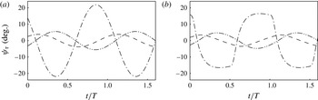
A generalization of the wall forcing to arbitrary, but nonetheless time-periodic, waveforms has been undertaken by Cimarelli et al. (Reference Cimarelli, Frohnapfel, Hasegawa, De Angelis and Quadrio2013) in the context of fully turbulent channel flow. At the optimal parameters, sinusoidal forcing outperformed all other investigated waveforms. If the forcing parameters deviated from their global optimum, however, other forcing waveforms yielded better performance. For sinusoidal forcing, the time dependence of the shear angle,
 $$\begin{eqnarray}{\it\psi}_{{\it\tau}}\equiv \arctan \left(\left.\frac{\partial W}{\partial y}\right/\frac{\partial U}{\partial y}\right),\end{eqnarray}$$
in planes parallel to the wall is also sinusoidal, and there exist intervals of slowly varying
 ${\it\psi}_{{\it\tau}}$
(see figure 26
a). In their investigation of fully turbulent channel flow, Touber & Leschziner (Reference Touber and Leschziner2012) remarked upon the importance of this state of lingering shear strain. They asserted that the very slow reorientation of the shear during phases of lingering allows turbulent streaks sufficient time to amplify in the instantaneous direction of the shear-strain vector. Touber & Leschziner (Reference Touber and Leschziner2012) concluded that drag reduction is undermined if the duration of the lingering state exceeds the time span for the generation of streaks.
Shear angle
 ${\it\psi}_{{\it\tau}}$
versus the phase of the base flow at
 $x=170$
and
 $y/{\it\delta}(x)=0.20$
(dashed-dotted),
 $y/{\it\delta}(x)=0.45$
(dashed) and
 $y/{\it\delta}(x)=0.70$
(dashed-double dotted). (a) Sine wave. (b) Square wave.

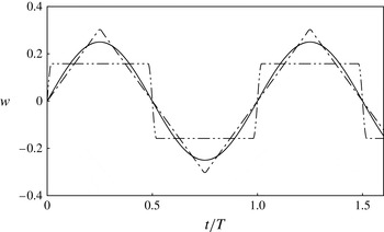
Additional flow simulations with triangle and square waveforms for the wall velocity were performed, and their influence on transition was determined. A continuously differentiable expression for the triangle wave is given by the Fourier series
 $$\begin{eqnarray}W_{triangle}(y=0,t)=\frac{8}{{\rm\pi}^{2}}\mathop{\sum }\limits_{k=0}^{\infty }\frac{(-1)^{k}}{(2k+1)^{2}}\sin \left((2k+1)\frac{2{\rm\pi}}{T}t\right),\end{eqnarray}$$
from which the first 16 terms were retained. A graphical representation of this approximation is given by the dashed-dotted line in figure 27. A Fourier expansion of the square wave, on the other hand, suffers from Gibbs oscillations. Therefore, the square wave was instead approximated by the following
 $C^{1}$
differentiable form,
 $$\begin{eqnarray}W_{square}(y=0,t)=\left\{\begin{array}{@{}ll@{}}\displaystyle W_{0}\sin \left(2{\rm\pi}\frac{t}{4a}\right),\quad & 0<t\leqslant a,\\ W_{0},\quad & a<t<T/2-a,\\ \displaystyle W_{0}\sin \left(2{\rm\pi}\left(\frac{1}{2}-\frac{T}{8a}+\frac{t}{4a}\right)\right),\quad & T/2-a\leqslant t\leqslant T/2+a,\\ -W_{0},\quad & T/2+a<t<T-a,\\ \displaystyle W_{0}\sin \left(2{\rm\pi}\left(1-\frac{T}{4a}+\frac{t}{4a}\right)\right),\quad & T-a\leqslant t\leqslant T,\end{array}\right.\end{eqnarray}$$
where the constant
 $a$
is small compared to the oscillation period,
 $a=0.02T$
. The resulting wall-oscillation profile is shown as the dashed-double dotted line in figure 27, and the shear angle is provided in figure 26(b). At
 $y/{\it\delta}(x)=0.20$
, the behaviour of
 ${\it\psi}_{{\it\tau}}$
still resembles the square wave at the wall. For larger wall distances, the phase dependence of the shear angle approaches a sine wave.
Spanwise velocity component at the wall,
 $w(0,t)$
, normalized to identical forcing power requirement,
 $\overline{P_{forcing}}$
: sine wave (solid), triangle wave (dash-dotted) and square wave (dash-double dotted).

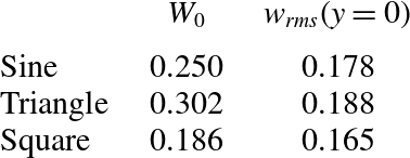
The forcing amplitudes were chosen such that the power requirements in the laminar region are in all cases equal to that of the sinusoidal forcing. The respective amplitudes and r.m.s. of the spanwise velocity at the wall are provided in table 1.
Properties of forcing waveforms for identical power input,
 $\overline{P_{forcing}}$
.

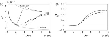
Variation of the forcing waveform: reference simulation (solid); sine wave (dashed); triangle wave (dash-dotted); square wave (dash-double dotted). (a) Skin friction coefficient
 $C_{f}$
over downstream Reynolds number
 $\mathit{Re}_{\tilde{x}}$
. (b) Net energetic advantage
 $\overline{P_{net}}$
over downstream Reynolds number
 $\mathit{Re}_{\tilde{x}}$
.

Flow simulations were performed for all three forcing profiles and an oscillation period
 $T=200$
. All other parameters, including those of the free-stream turbulence at the inlet were unchanged. The skin friction coefficient is plotted in figure 28(a), and demonstrates that forcing with the triangle wave yields nearly identical results to the sinusoidal oscillation. Application of the square wave, on the other hand, preserves laminar flow farther downstream, up to
 $\mathit{Re}_{\tilde{x}}\approx 3.8\times 10^{5}$
. The energetic balance is reported in figure 28(b). Since the power input is identical in all cases, the net power savings are directly related to the reduction in propulsion power,
 ${\rm\Delta}\overline{P_{prop}}$
. The downstream shift in transition location in the case of the square wave leads to an increase in
 $\overline{P_{net}}$
by approximately 20 % at a Reynolds number
 $\mathit{Re}_{\tilde{x}}\approx 6.2\times 10^{5}$
.
The results establish that the sudden change of the spanwise velocity in the case of the square wave stabilizes the laminar flow regime more effectively than the sinusoidal forcing. Since the swift change in
 $W(0,t)$
is the high-frequency part of the wall motion, its influence decays quickly in
 $y$
, and a sinusoidal time dependence is recovered away from the wall (cf. figure 26). Nearer to the wall, however, the form of the square wave is still discernible and more effectively delays the onset of transition.
The discussion in this section highlights two observations: First, an increase in the oscillation amplitude does not necessarily enhance stability, and can in fact cause transition to shift farther upstream than the reference flow. Second, the sinusoidal wall oscillation did not yield the best performance, for a fixed power input. Both these trends should be compared to the literature on drag reduction in fully turbulent flows where (i) an increase in the amplitude of wall oscillation enhances drag reduction and (ii) the sine wave is the optimal forcing waveform. As such, while the current study was originally motivated by previous work on fully turbulent configurations, the influence of the wall motion on transition is markedly different.
7. Conclusions
The potential to affect bypass breakdown to turbulence via time-harmonic wall forcing was investigated by means of DNS. For suitable forcing parameters, the onset of transition can be shifted downstream appreciably, and the length of the transition region can be significantly extended. It was also demonstrated that the decrease in theoretical propulsion power due to the delay of the fully turbulent flow significantly outweighs the power requirement of the wall forcing.
The transition process is sensitive to the forcing parameters. Starting with very short periods of oscillation, an increase in
 $T$
enhances drag reduction until an optimum is reached. Longer periods rapidly diminish, and even reverse, the stabilization of the laminar regime. As a result, for periods of approximately twice the optimal value, transition occurs upstream of the unforced reference case. A qualitatively similar behaviour is observed when increasing the amplitude of the forcing beyond its optimal value. Analysis of the phase of spot inception showed that breakdown to turbulence in these cases is correlated with a particular phase of the wall forcing cycle. The focus, however, was placed on the optimal forcing parameters where transition was substantially delayed.
Instantaneous fields and statistical results demonstrated that the optimal oscillation frequency significantly weakened boundary-layer streaks in the pre-transitional flow. Sampling of the properties of large numbers of individual streaks demonstrated that the forcing leads to narrower distributions for the streak amplitudes of both high-speed and low-speed streaks. The averaged amplitudes of laminar streaks are reduced by up to 50 % in comparison to the reference case. In addition, linear stability analyses confirmed a substantial reduction of the growth rates of secondary streak instabilities in the presence of the forcing. These results explain the reduced frequency of occurrence of turbulent spots observed in the DNS.
Finally, a study of different waveforms for the spanwise wall forcing was performed. It was shown that, for identical power input into the wall movement, an oscillation described by a square wave can shift the onset of transition farther downstream than sinusoidal forcing. Apart from the increased efficiency, forcing with a square wave also demands a 40 % lower peak value of the spanwise wall velocity than sinusoidal forcing.