





Introduction
The Greenland ice sheet is a prominent frozen reservoir of freshwater on Earth. In recent decades, it has had a negative mass balance, losing more ice through melt, runoff and iceberg calving than it gains each year through snow accumulation that gradually compacts into ice (Mouginot and others, Reference Mouginot2019; Mankoff and others, Reference Mankoff, Solgaard, Colgan, Ahlström, Khan and Fausto2020). Although widespread satellite observations in recent years have improved the monitoring of overall mass loss of the Greenland ice sheet (Shepherd and others, Reference Shepherd2012; Hanna and others, Reference Hanna2013; Mouginot and others, Reference Mouginot2019; Smith and others, Reference Smith2019), gaps remain in scientific understanding of the physical processes governing dynamics of the ice sheet and how these will impact mass loss in the future. A particular source of uncertainty in future sea level projections associated with ice mass loss is the role of subglacial hydrology, or liquid water at the interface between the ice and the underlying bed material. The subglacial environment is difficult to access for direct observations, but numerical models can provide insights into basal processes by simulating the relevant physical processes of water and ice flow, melt, and sliding.
Subglacial hydrology affects the velocity of glaciers by modulating how easily the ice slides over its bed. Glacier sliding parameterizations (or ‘sliding laws’) are generally formulated in terms of basal stress, calculated as a function of ice sliding velocity and effective pressure, which is defined as the difference between ice overburden pressure and water pressure at the bed (Budd and others, Reference Budd, Keage and Blundy1979; Schoof, Reference Schoof2005). The specific relationship and exponents vary between different sliding laws, but sliding velocity and effective pressure typically have a nonlinear relationship.
Water below glaciers flows according to pressure gradients, which are partly determined by geometric properties of the glacier, such as surface slope, ice thickness and bed slope, and partly by fluid flow dynamics. Pressure evolves dynamically through space and time with evolving glacier geometry and hydraulic processes. Water moves from high to low pressure, meaning that in some cases water can flow uphill relative to the bed or surface topography. Although bed topography beneath the ice is difficult to accurately constrain, ice surface elevation has been relatively well observed since 2003 with NASA’s Ice, Cloud and land-Elevation satellite (ICESat) and follow-up Operation IceBridge (MacGregor and others, Reference MacGregor2021) and ICESat-2 laser altimetry missions, by which the travel time of laser pulses is used to measure the elevation of Earth’s surface (Schutz and others, Reference Schutz, Zwally, Shuman, Hancock and DiMarzio2005; Abdalati and others, Reference Abdalati2010; Markus and others, Reference Markus2017). Changes in ice surface elevation and surface slope cause changes in the hydraulic pressure gradient at the bed.
Liquid water beneath glaciers is derived from melting at the base of the ice as well as seasonal surface melting that drains through the ice. During the winter months, the subglacial system receives water primarily from basal melt and is in a relatively stable background state. During the summer months, a significant fraction of the water that melts on the surface of the ice sheet drains to the bed via moulins and crevasses (Meierbachtol and others, Reference Meierbachtol, Harper and Humphrey2013; Andrews and others, Reference Andrews2014; Smith and others, Reference Smith2015). At higher elevations, a portion of surface melt percolates into porous firn and refreezes instead of running off (Meyer and Hewitt, Reference Meyer and Hewitt2017; Rennermalm and others, Reference Rennermalm2022). Intuitively, one might expect that more meltwater being produced on the ice sheet would lead to more water at the bed, and a corresponding increase in water pressure and acceleration. However, this is not necessarily the case—as has been observed through field observations and represented in numerical models (Schoof, Reference Schoof2010; Flowers, Reference Flowers2015)—with sufficient meltwater inputs to the bed, the drainage system will transition to form an efficient system of channelized pathways. These efficient conduits decrease water pressure and consequently pull water from the surrounding bed, increasing friction and yielding a deceleration even with increasing melt (Sundal and others, Reference Sundal, Shepherd, Nienow, Hanna, Palmer and Huybrechts2011). This negative feedback complicates predicting future development of Greenland glacier seasonal velocities, and numerous scientific studies have attempted to understand when and where such channelized drainage is likely to develop (Banwell and others, Reference Banwell, Hewitt, Willis and Arnold2016; Cowton and others, Reference Cowton, Nienow, Sole, Bartholomew and Mair2016; Simkins and others, Reference Simkins, Greenwood, Munevar Garcia, Eareckson, Anderson and Prothro2021; Rada Giacaman and Schoof, Reference Rada Giacaman and Schoof2023; Warburton and others, Reference Warburton, Meyer and Sommers2024).
In this study, we are motivated by questions that address the impact of the background state and seasonal evolution of the subglacial system: (1) How do decadal-scale changes in surface elevation influence changes in winter background state subglacial hydrology and corresponding ice dynamics of the Greenland ice sheet? (2) How much is seasonal velocity attributable to glacier geometry compared to environmental forcing? Leveraging ice surface elevation derived from ICESat and ICESat-2 observations, we use a coupled subglacial hydrology–ice dynamics model to simulate changes in effective pressure and ice velocity over the period 2004–20.
In the following sections, we describe our methods, including how we generate our high-resolution digital elevation models (DEMs), the models and data we use, and our experimental approach. We then present simulation results and discuss implications of our findings.
Methods
DEM generation
We generate high-resolution DEMs of the Greenland ice-sheet surface based on a combination of ICESat and ICESat-2 satellite laser altimetry, Operation IceBridge airborne laser-altimetry data, and ArcticDEM digital elevation models. We combine these using a surface-fitting algorithm adapted from the algorithm developed for the ICESat-2 ATL14 and ATL15 gridded height and height-change data products, with additional processing steps added to help correct for potential artifacts in the other datasets. The ATL14/15 algorithm (Smith and others, Reference Smith, Jelley, Dickinson, Sutterley, Neumann and Harbeck2025; Reference Smith2026) approximates ice-sheet elevations as the sum of a fine-resolution reference DEM and a set of coarser-resolution elevation-change surfaces. For example, the ICESat-2 project generates a 100 m DEM (ATL14) and a set of elevation-change surfaces with 1 km horizontal and 0.25 year temporal resolution. The algorithm works by minimizing a functional that depends on the roughness of the DEM, the roughness of the elevation-change rate described by the elevation-change surfaces, and the uncertainty-scaled misfit between the estimated elevation (equal to the sum of the DEM and the elevation-change surfaces) and the ICESat-2 data points. The combined ATL14 and ATL15 data products give well-constrained estimates of surface height during the ICESat-2 mission (2019–25) along reference ground tracks that ICESat-2 has measured repeatedly, but the accuracy of the surface-height estimates declines in the gaps between these tracks (Smith and others, Reference Smith2026). We use a modified version of this algorithm with an extended set of input data products to generate a set of high-resolution DEMs spanning 2004–20.
Our DEM generation is carried out in two stages. In the first stage, we apply the surface-fitting algorithm to a combination of ICESat-2 and ArcticDEM data to generate a high-resolution (50 m) DEM referenced to decimal year 2020.5. In the second stage, we subtract this DEM from a multi-decadal time series of ICESat and IceBridge laser-altimetry data to produce a set of elevation-difference measurements spanning 2004–20. We then apply the surface-fitting algorithm to these difference measurements to produce a time series of gridded elevation differences with 500 m horizontal and 1 year temporal node spacing. See the Supplementary Material for more details about generating the reference 2020 DEM and estimating surface elevation for subsequent snapshots at 2004, 2008, 2012, 2016 and 2020.
Model description
To simulate subglacial hydrology, we use the Subglacial Hydrology And Kinetic, Transient Interactions model (SHAKTI; Sommers and others (Reference Sommers, Rajaram and Morlighem2018)) coupled with ice dynamics in the Ice-sheet and Sea-level System Model (ISSM; Larour and others (Reference Larour, Seroussi, Morlighem and Rignot2012)). SHAKTI is a physics-based model that calculates evolving hydraulic head, effective pressure, subglacial gap height, water flux and basal melt. The model internally calculates spatiotemporally variable hydraulic transmissivity, allowing for turbulent, laminar, and transitional flow regimes to develop, and flexible drainage geometries to emerge that represent a continuum from inefficient/distributed drainage, to efficient/channelized drainage. ISSM is a state-of-the-art glacier ice flow model that uses finite element methods on adaptable meshes to simulate a variety of processes that impact ice dynamics. SHAKTI is built into ISSM as a module to facilitate coupling between subglacial hydrology and ice velocity, which occurs through the friction parameterization, or sliding law, in which basal stress depends on both effective pressure (calculated by SHAKTI) and ice sliding velocity (calculated by the stress balance in ISSM). We use the same form of the SHAKTI equations as in Sommers and others (Reference Sommers2024). The simulations presented in this paper use the Budd-type sliding law (Budd and others, Reference Budd, Keage and Blundy1979) and the Shallow Shelf Approximation (SSA) (MacAyeal, Reference MacAyeal1989) for ice flow. See Table S1 for a list of parameter values.
In the Budd friction parameterization, basal stress  $\tau_b$ is calculated as:
 \begin{equation}\tau_b=C^2 N u_b,\end{equation}
where  $C$ is a spatially variable friction coefficient,
 $N$ is effective pressure and
 $u_b$ is ice sliding velocity (which is equivalent to the depth-integrated velocity in the SSA ice flow approximation used here).
In an effort to keep the model relatively simple while including hydrology and velocity coupling, we assume an average bulk ice temperature of  $-$10
 $^\circ$C for the entire domain, with ice rheology (Glen’s flow law coefficient) based on that temperature. This same rheology applies to SHAKTI and appears in the creep closure of the subglacial system, which depends on the flow law parameter. The basal melt rate calculation implicitly assumes that water and ice directly at the bed are both at the pressure melting point. No-flux Neumann boundary conditions are applied along the domain boundaries, and a Dirichlet boundary condition setting hydraulic head to zero is applied to ice-free nodes and where ice thickness is less than 10 m. Assuming that fjord water is well mixed with fresh water near the terminus of marine-terminating glaciers, this sets the subglacial discharge water pressure equal to the hydrostatic pressure of the overlying water depth in the fjord at the terminus. We begin with an initial subglacial gap height of 0.01 m and use a time step of 1 hour.
Our model domain is a region in northwest (NW) Greenland (Fig. 2a), selected as a focus area because of its significant change in surface elevation and numerous fjords with outlet glaciers. The finite element mesh consists of 129 273 triangular elements, using adapted resolution based on observed surface velocity, with element edge lengths ranging from 100 m to 20 km. We use ice thickness and bed elevation estimates from BedMachine v5 (Morlighem and others, Reference Morlighem2021) to set the ice geometry for 2004. Bed elevation is held consistent for all other years, while the ice thickness changes corresponding to changes in ice surface elevation. After prescribing the 2004 ice geometry for our domain, we perform an inversion to infer the pattern of the spatially variable friction coefficient  $C$ used in Eqn (1), assuming in the inversion perfect connectivity to the ocean (i.e. hydraulic head equals zero and effective pressure is purely a function of ice geometry). This is similar to the iterative inversion initialization process described in Sommers and others (Reference Sommers2024) but with only one inversion. In standard practice ice sheet modeling, the friction coefficient is typically used to represent the lumped influence of variable conditions at the bed necessary to reproduce observed velocity patterns, including variations in effective pressure. Because we explicitly account for spatial and temporal variations in effective pressure in our coupled hydrology simulations, here the friction coefficient primarily represents variations in bed material properties that influence basal friction and presumably remains relatively unchanged over the decadal time scales considered here. We hold this friction coefficient distribution consistent in all our simulations, and the basal stress obviously evolves with changes in effective pressure. This is in contrast to the transient calibration approach of Badgeley and others (Reference Badgeley, Morlighem and Seroussi2025), for example, in which sequential inversions are performed to infer changes in friction coefficient, assuming a static effective pressure distribution.
Winter background hydrology and velocity
We run coupled SHAKTI–ISSM spin-up simulations for 1 year to generate the winter ‘background state’ hydrology and velocity conditions for snapshots at 2004, 2008, 2012, 2016 and 2020, with ice geometry based on the derived DEM for each year described above. Ice geometry remains unchanged during each simulation, with surface elevation set by the DEM for each year. Ice thickness and terminus positions do not transiently evolve during a simulation. In these winter simulations, we assume that all meltwater present in the subglacial system is produced by basal melt through a combination of geothermal flux, frictional heat from sliding and turbulent dissipation. The winter background sets the initial conditions for the melt season in Greenland, with drainage structures sustained below the ice even in the absence of large surface meltwater inputs. Far from being stagnant, active subglacial hydrological systems persist through the winter, supplied by basal melt (Sommers and others, Reference Sommers2023).
Seasonal simulations
Beginning from our winter background state simulations for 2004 and 2020, we run transient seasonal simulations using ice sheet surface runoff derived from the MERRA-2 climate reanalysis (Gelaro and others, Reference Gelaro2017) to prescribe the magnitude, timing and distribution of meltwater inputs to the bed. We direct all surface runoff immediately to the bed at the location where the water is produced, neglecting the nuances of routing, refreezing or storage in the supraglacial and englacial drainage systems. In order to uniquely assess the role of surface geometry in determining hydrological and ice flow under comparable environmental forcing, we force these transient simulations on 2004 and 2020 geometries using the same seasonal runoff data from the mean climatology over the period 2003–22.
Ice velocity comparison to observations
In order to assess the impact of surface elevation change on ice velocity patterns relative to observations, we compare the modeled winter background states to winter time SAR-derived ice velocities (Joughin and others, Reference Joughin, Smith, Howat, Scambos and Moon2010; Reference Joughin, Smith, Howat and Scambos2015; Reference Joughin, Smith and Howat2018; Joughin, Reference Joughin2023). To complete this analysis, we use observations dated from 2000 to 2020; 2000 is used because the next image is from 2005/2006. Table S2 presents a list of the specific images used. Velocity images span variable ranges, but do not include the summer melt season (June, July and August). We then calculate the linear velocity trend of each pixel. Using the linear trend, we determine the expected velocity at the model time steps of 2004.5 and 2020.5. We perform the same analysis for the winter background model outputs after regridding the model outputs to the observational grid of 500 m  $\times$ 500 m. This processing permits us to directly compare the observations and model outputs while minimizing the impact of interannual variability.
Model results
Figure 1 presents ice surface velocity, subglacial water flux and effective pressure modeled using 2004 and 2020 surface elevations. Modeled velocity, water flux and effective pressure all vary spatially, and overall display the same large-scale structure in both years. The differences between the two, however, reveal notable changes attributable to changes in surface elevation. These changes are discussed next.
Model domain in NW Greenland and modeled ice velocity in (a) 2004 and (b) 2020. Modeled subglacial water flux in (c) 2004 and (d) 2020. Modeled effective pressure in (e) 2004 and (f) 2020. All  $x$ and
 $y$ axes are in polar stereographic projection (EPSG: 3413) with units of km.

Ice surface elevation changes
Figure 2a shows the difference in ice surface elevation (2020  $-$ 2004) over the Greenland ice sheet as observed by the ICESat and ICESat-2 missions, based on the DEMs described above. Significant elevation decrease (i.e. ice sheet thinning) is visible around the margins of the ice sheet, and no significant increase in surface elevation is apparent. Some major outlet glaciers show large areas of pronounced surface lowering in excess of 100 m over this period, with widespread thinning along the NW coast. Incremental changes every 4 years over this period are presented in Figs S1 and S2, with a general pattern of steady thinning around the ice sheet margins over each segment of time.
(a) Change in ice surface elevation (2020 minus 2004) over the Greenland ice sheet, with model domain in NW Greenland. (b) Modeled change in background state subglacial water flux, (c) effective pressure and (d) ice velocity. (e) Modeled change in total basal melt rate. (f) Modeled change in basal melt rate due to frictional heat and (g) dissipation.

Changes in winter water flux, effective pressure, velocity and basal melt
Figure 2b–g present spatial plots of modeled changes in winter subglacial water flux, effective pressure, ice velocity and basal melt rate as simulated by the coupled model SHAKTI–ISSM for the ICESat (2004) and ICESat-2 (2020) eras in NW Greenland, with changes plotted as the difference between these results (2020 minus 2004). Incremental changes every 4 years over this period are presented in Figs S2–S5. Changes in subglacial water flow paths caused by changes in surface elevation are clearly visible as blue and red pathways in Fig. 2b. Red indicates a decrease in winter water flux and blue indicates an increase in winter water flux over the period 2004–20. The difference between 2020 and 2004 shows a mix of increases and decreases in water flux at different places. Incremental 4 year simulation steps suggest that background water flux generally increased in the interior from 2004 to 2008 with some notable switches in subglacial water flow paths, further reorganized between 2008–12 and 2012–16, and experienced more of an overall decrease from 2016 to 2020 (Fig. S2), resulting in the full mixed reconfiguration apparent in Fig. 2b. For a closer view of the redirection of water flux, percent change in modeled subglacial water flux is shown in Fig. 3a, d and g for three selected areas.
(a, d, g) Percent change in modeled background subglacial water flux, (b, e, h) effective pressure and (c, f, i) ice velocity between ICESat (2004) and ICESat-2 (2020) eras, zoomed in for detail in three areas shown on Fig. 2a.

Modeled effective pressure reveals a consistent decrease in effective pressure near the margin (red), with a general increase in effective pressure in the interior (Fig. 2c). A closer look is provided at the percent change in modeled effective pressure in Fig. 3b, e and h. These changes, however, do not develop through a linear progression, as seen in the 4 year incremental change plots in Fig. S3, but rather exhibit more widespread changes in effective pressure during the 2004–08 and 2016–20 periods, with relative stability during 2008–12 and 2012–16, except for localized increases in effective pressure.
Simulated velocities show deceleration in some outlet glaciers near the margin, while others accelerate, and overall a dominating acceleration trend further inland over the full period 2004–20 (Fig. 2d), with a zoomed-in perspective for detail of percent change in velocity in Fig. 3c, f and i. When viewed over 4 year increments, again these patterns of change do not develop linearly over time, but instead show up with mixed acceleration and deceleration during 2004–08 (Fig. S4). From 2008–12 and 2012–16, the modeled velocity change continues to be mixed, with areas of acceleration and deceleration. The period 2016–20 shows a broad pattern of mild deceleration in the interior with pronounced acceleration in several outlet glaciers.
As calculated by SHAKTI, our simulations suggest a variety of changes in basal melt rate (Fig. 2e) between 2004 and 2020, with locations near the margin experiencing reduced basal melting, and a clear increase in basal melt inland. The bulk of the change in basal melt rate is attributable to changes in frictional heat associated with changes in sliding velocity (Fig. 2f). However, turbulent dissipation corresponding to changes in subglacial water flux is significant at some outlet glaciers, leading to increased basal melt from dissipation in places where winter water flux increased or was redirected (Fig. 2g).
Through examination of changes in ice velocity, effective pressure, basal melt rate and subglacial water flux as related to changes in ice surface elevation (Fig. 4), a trend emerges relating a decrease in modeled effective pressure with a decrease in surface elevation (Fig. 4b). However, the relationship is weak for predicting changes in modeled velocity or basal melt rate based on changes in surface elevation (Fig. 4a, c and d). An overall relationship between increasing ice velocity and increasing effective pressure is apparent (Fig. 4e). This is perhaps counter-intuitive, as a decrease in effective pressure with ice thinning might be presumed to imply an increase in velocity. The modeled data, however, display a high degree of variability and generally suggest a lack of predictability of ice velocity response to projected ice thinning. We also note that thinner ice does not necessarily imply decreased effective pressure, since the water pressure evolves in response to those changes and does not remain constant, and the ice surface does not lower uniformly everywhere. Coupled simulations such as these provide a window into the nonlinear and complicated behavior of ice sheet dynamics.
(a) Modeled change in ice velocity, (b) change in effective pressure, (c) change in basal melt rate and (d) change in subglacial water flux as a function of change in ice surface elevation. (e) Modeled change in velocity as a function of change in effective pressure. Solid dark lines show a linear fit, with  $\pm$95% confidence plotted in light dashed lines.

Response to seasonal melt
Figure 5 presents time series of mean modeled effective pressure, subglacial water flux, ice velocity and total basal melt over our model domain in response to seasonal meltwater forcing based on mean 2003–22 climatology derived from MERRA-2 reanalysis as described above. For both the 2004 and 2020 geometries, subglacial water flux increases during the melt season in response to the runoff inputs. This generally corresponds to an increase in velocity and decrease in effective pressure early in the melt season, followed by deceleration and an increase in effective pressure following the peak of the melt season at Day 200. Notably, an abrupt acceleration near the end of the melt season corresponds with a decrease in effective pressure as the drainage system shuts down and becomes less efficient. Overall, the shape of the response is similar in both simulations, but with an offset in effective pressure and velocity between the background winter state for the two eras, reflecting a general decrease in both effective pressure and ice velocity in 2020 as compared to 2004, simply due to the differences in ice surface elevation. While the response is qualitatively similar, the difference between the two seasonal simulations (2020 minus 2004; Fig. 5d–f) reveals some variation around the background offset, with a slightly less negative response in effective pressure during the peak melt season in 2020 compared with 2004, a slightly more negative response in water flux and a slightly less negative response in velocity. The relationship between the spatial mean modeled quantities in these seasonal simulations using the 2004 and 2020 geometries is plotted in Fig. 5g–i, showing a near-linear pattern, but with some variation around that. These results show that changes in ice geometry and the background subglacial drainage state influence the seasonal response in coupled behavior of the Greenland ice sheet, again highlighting the complex response of the ice sheet to changes in surface elevation.
(a) Mean runoff forcing from 2003–22 mean MERRA-2 climatology, (b) mean modeled effective pressure, (c) subglacial water flux, (d) ice velocity and (e) total basal melt in response to seasonal meltwater forcing with ice geometry corresponding to the ICESat era (2004; blue) and ICESat-2 era (2020; red). (f) Difference (2020 minus 2004) in mean effective pressure, (g) mean subglacial water flux, (h) mean ice velocity and (i) total basal melt. (j) Relationship of mean effective pressure, (k) water flux and (l) velocity between 2004 and 2020 simulations. (m) Change in modeled ice velocity during peak melt season (Day 200) relative to modeled winter ice velocity with 2000 ice elevation and (n) 2020 ice elevation.

Discussion
Changes in subglacial water flow
Our simulation results show an increase in subglacial water in some areas (appearing blue in Figs 2b and 3a, d and g) and a reduction in others (appearing red in Figs 2b and 3a, d and g). The relationship between change in water flux and change in surface elevation is relatively weak when considered over the entire model domain (Fig. 4d). However, some locations suggest an increase in subglacial water being produced and routed toward areas that have experienced enhanced thinning, with a reduction in water flow toward outlets that have maintained relatively more of their thickness (Fig. 2). Local changes in subglacial water flow not only influence ice sliding velocity by changing the pressure distribution at the bed, but also hold ramifications for freshwater discharge into fjords along the margins of the ice sheet. Changes in freshwater flux may have wide-ranging impacts such as changes in fjord circulation patterns, ecology, biogeochemistry, frontal melt rates and terminus position (Straneo and Cenedese, Reference Straneo and Cenedese2015; Jackson and Straneo, Reference Jackson and Straneo2016; Sejr and others, Reference Sejr2022; Vries and others, Reference Vries, van de Berg, Noël, Meire and van den Broeke2025).
Interior acceleration
We simulate a general decrease in effective pressure near the ice sheet margins, but a modest increase in effective pressure further inland, which corresponds to an overall accelerating trend in simulated winter ice velocity between 2004 and 2020 (Fig. 2c and d). This result may initially seem surprising. If basal conditions remained the same in terms of water pressure, a decrease in ice thickness would lead to a decrease in effective pressure and corresponding acceleration. Our simulations demonstrate a more mixed response. Changes in surface gradients facilitate a reorganization of pressure gradients at the bed that drives the reconfiguration of subglacial water flow and corresponding changes in pressure. These various factors play out in different ways under different specific conditions, and it is worth noting the widespread interior acceleration that occurs even with deceleration in certain locations near the ice sheet margin.
To explore the relative controls on ice velocity changes, we investigate the importance of the redistribution of subglacial water flux (and corresponding changes in effective pressure) as compared to the change in driving stress due to thinning and changing surface slopes. In order to do this, we take the effective pressure distribution resulting from our 2004 simulation, use that effective pressure with the 2020 geometry and calculate the ice velocity from the stress balance under these conditions. The differences in velocity are shown in Fig. S6. While the patterns of change in velocity near the ice-sheet margin are complicated, the interior acceleration is more pronounced in this experiment that separates the control of driving stress changes from the influence of hydrological changes. This suggests that the hydrological impact actually compensates for what would otherwise be larger interior acceleration due to geometry and corresponding driving stress changes alone.
Comparison to velocity observations
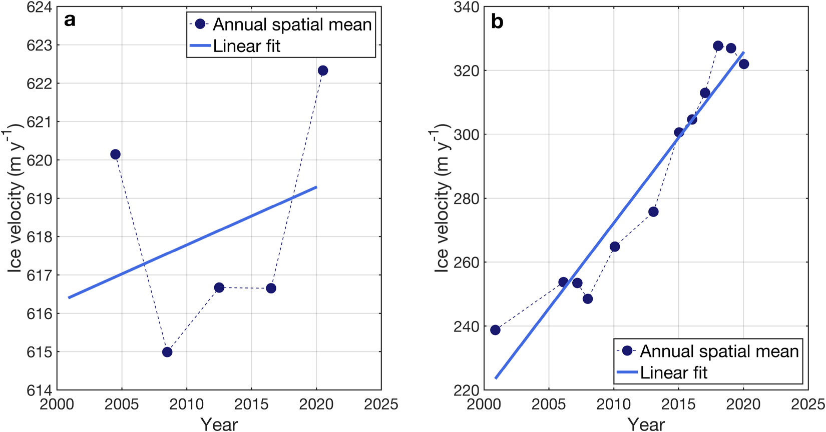
We compare our modeled changes in velocity to observed changes in velocity using winter observations derived from synthetic aperture radar (SAR) over the same period. Figure 6 shows the calculated change in velocity over time, averaged per year in modeled and observed velocities, and the number of available winter velocity observations at each location. In general, the model and observations show a similar pattern, with the exception of the very near-terminus regions. However, the magnitude of the change in velocity over time is lower in the model than in the observational dataset. Figure 7 shows the percent change in velocity over the period between 2020 and 2004, as modeled and observed, and the difference between them. The annual trend in mean modeled and observed velocity is presented in Fig. 8, showing a general acceleration. Overall, modeled velocity changes reproduce the observed spatial patterns, but the magnitude of change between 2020 and 2004 is only about 20% of the observed change in velocity. Our winter background modeling approach accounts for changes in surface elevation and changes in subglacial hydrology, isolating these influences from other sources of influence at the terminus such as changes in warm water circulation, changes in terminus position and buttressing support, and other ice/ocean interactions, along with changes in seasonal surface melt. The fact that the model produces velocity changes that generally agree spatially with observations is encouraging, and we interpret this to represent the magnitude of velocity change that can be attributed to changes in ice surface elevation and corresponding changes in the subglacial hydrological system.
(a) Change in velocity over time as modeled due to change in surface elevation and hydrologic effects. The change in velocity over time is calculated as 2020 velocity minus 2004 velocity, divided by 16 years. (b) Change in observed velocity over time. (c) Count of available velocity observations derived from SAR.

(a) Percent change in velocity (2020 minus 2004) as modeled due to change in surface elevation and hydrologic effects. (b) Percent change in observed velocity (2020 minus 2004). (c) Difference between observed and modeled percent change in velocity.

Mean winter ice velocity and linear regression trend based on (a) modeled and (b) observed velocities.

Basal melt changes
Ice-sheet mass balance is estimated from melting at the surface, but the ice also melts from below at the ice–bed interface. The role of basal melting has recently been highlighted as an important consideration for overall ice-sheet mass balance (Karlsson and others, Reference Karlsson2021; Young and others, Reference Young2022), although it is difficult to observe directly and constrain over large time and space scales. SHAKTI calculates total basal melt rate, along with its components (geothermal, frictional and turbulent heat), providing an informed estimate of evolving basal melt. As shown in Fig. 2, changes in ice elevation yield heterogeneous changes in basal melt rate in the coupled SHAKTI–ISSM model. In the interior, these changes are dominated by changes in frictional heat, whereas changes in dissipation are important at the outlets, especially in places where subglacial water flux has increased or decreased through hydrologic reorganization as a result of changes in surface elevation.
Our coupled winter simulations calculate a total background basal melt volume over our model domain of 11.72 Gt yr $^{-1}$ in 2004 and 11.77 Gt yr
 $^{-1}$ in 2020. This implies an increase of 0.05 Gt yr
 $^{-1}$ in background basal melt in this region.
Importance of the winter background state
Changes in ice surface elevation alone alter the pattern of basal melting and, over the 2004–2020 interval, result in substantial changes in the subglacial winter background state. Our seasonal simulation results (Fig. 5) suggest that the winter background state has a non-negligible influence in determining pressure and velocity magnitudes. The winter background state is determined by ice geometry that has shifted over time on a decadal scale between the eras of ICESat and ICESat-2 observations. It is notable that the seasonal pressure and velocity responses in our seasonal simulations using 2004 and 2020 geometries are offset based on the winter background state when forced with the same transient runoff inputs to the bed, but also exhibit differences in the magnitude of response during the melt season (Fig. 5). While in reality, seasonal forcing evolves over time and also exhibits interannual variability, this modeled exercise allows for isolation of the difference in response due to geometry alone. It is also perhaps unexpected that the ICESat-2 era displays both a decrease in mean modeled effective pressure and mean modeled velocity, as one might expect that a decrease in effective pressure should lead to increased velocity. The key here is that these quantities are mean values over the entire domain; although our simulations produce an increase in effective pressure in the interior, we calculate substantial decreases in effective pressure along the margins, which act to significantly lower the mean value of change in effective pressure. These findings demonstrate the complex impact of changes in surface elevation and the resulting response in ice dynamics, when accounting for the coupled effects of subglacial hydrology.
Limitations
As in any modeling effort, we made informed choices of parameter values and approximations to physics, including choices for ice temperature and rheology, flow law approximation, sliding law, process parameterizations and forcing data. We cannot and do not aim to perfectly reproduce reality with all its complexities, but we do aspire to represent the relevant physical processes in an appropriate way to assess feedbacks and make inferences about realistic behavior of the Greenland ice sheet. In the landscape of coupled subglacial hydrology and ice dynamics modeling, much remains for future work to rigorously assess the impact of different sliding laws and improve parameterization of basal friction with evolving hydrology. For example, McArthur and others (Reference McArthur, McCormack and Dow2023) found that the Schoof friction law produced better velocity results than the Budd friction law in coupled modeling of an Antarctic glacier using a different subglacial hydrology model, and Meyer and others (Reference Meyer, Warburton, Sommers and Minchew2026) compared coupled simulations using SHAKTI–ISSM with both Budd and Schoof friction laws at Thwaites Glacier.
At least in the early part of our study period (2004–09), the resolution of our elevation-change maps is limited by the track-to-track spacing of the ICESat data, which is up to 20 km in the southern part of our domain. This means that the elevation-change estimates may not resolve the fine details of surface-elevation change, and may underestimate gradients in elevation change around relatively small topographic features such as outlet glaciers.
We selected our model domain in NW Greenland based on its significant widespread surface elevation change between 2004 and 2020, representative of the ICESat and ICESat-2 eras (Fig. 2a). Future research should model larger regions of the Greenland ice sheet, ideally the entire ice sheet. The work presented here represents advances in coupled subglacial hydrology–ice dynamics modeling using SHAKTI–ISSM on a larger domain than previous applications to single glaciers. Further work should aim to expand these modeling capabilities and establish robust general boundary conditions that can easily be applied to any complicated ice sheet or glacier domain. Moreover, much remains to be explored regarding how best to represent sliding laws and geological friction coefficients while modeling coupled ice velocity and subglacial hydrology.
Conclusions
In this study, we present large-scale coupled subglacial hydrology and ice dynamics using SHAKTI and ISSM applied to NW Greenland. We find that changes in ice surface elevation, as observed by satellite laser altimetry from NASA’s ICESat and ICESat-2 missions and derived gridded products, yield changes in subglacial water flow and corresponding ice velocity, along with changes in basal melt rates. We find instances of increased subglacial water flow toward outlets with enhanced thinning and decreased water flow toward outlets that have retained more of their ice thickness. This reorganization of freshwater discharge holds potential impacts for fjord dynamics, biogeochemistry and ecology, as well as for frontal ablation rates (including both melt and calving processes). Our simulations demonstrate decreased effective pressure and locations of decreased ice velocity near the margins of the ice sheet, but conversely a modest increase in effective pressure and overall velocity acceleration in the interior. The changes in velocity due to changes in surface elevation and subglacial hydrology as computed by our coupled model are smaller than the observed velocity changes over this time period. This may be at least partially attributed to the neglect of changes in terminus forcing (e.g. changes in terminus position, buttressing, warm water circulation in fjords, etc.). Accompanied by an increase in simulated background basal melt rate, these results suggest feedbacks intensifying mass loss from the Greenland ice sheet attributable to changes in ice surface elevation and changes in the subglacial system. Changing the geometry alone yields a higher interior acceleration due to changes in driving stress than with coupled hydrological changes, indicating that the impacts from changing hydrology and basal stress help to soften the inland acceleration effect of changes in driving stress. The coupled simulations demonstrate the complexity and nuance in accounting for changes in effective pressure due to changes in subglacial hydrology, while highlighting how the ice sheet and its subglacial drainage system respond heterogeneously to changes in surface elevation.
Supplementary material
The supplementary material for this article can be found at https://doi.org/10.1017/jog.2026.10223.
Data availability statement
We used ISSM version 4.24. ISSM (including SHAKTI) is freely and publicly available for download at https://github.com/ISSMteam/ISSM. Model output data and code are available in a permanent Zenodo archive at https://doi.org/10.5281/zenodo.21266719.
Acknowledgements
This study was supported by NASA grants 80NSSC23K1329 and 80NSSC23K0937. We thank Scientific Editor Ian Hewitt and the reviewers for their helpful comments.




 Open access

