

Introduction
Perhaps the most striking feature of communities of either free-living (Gaston, Reference Gaston1994; Gaston & Blackburn, Reference Gaston and Blackburn2000) or parasitic (Poulin, Reference Poulin2007) organisms is that a few species tend to be very abundant whereas most other species are much less common, some being very rare. The pattern is not universal, of course: in some communities, one or very few species account for the vast majority of individuals in the community, whereas in others there is greater evenness in the abundance of different species (Poulin, Reference Poulin1996). The concept of numerical dominance has been widely used in parasite community ecology to label the most abundant species (e.g. Salgado-Maldonado & Kennedy, Reference Salgado-Maldonado and Kennedy1997; Gutiérrez, Reference Gutiérrez2001; Sures & Streit, Reference Sures and Streit2001; Schabuss et al., Reference Schabuss, Kennedy, Konecny, Grillitsch, Schiemer and Herzig2005). The related concept of core and satellite species, similarly based on abundance, also has a long history in parasite community ecology (see Holmes & Price, Reference Holmes, Price, Anderson and Kikkawa1986; Sousa, Reference Sousa1994). However, these concepts have been mostly used as descriptive tools to classify some species as dominant and others as rare, based on arbitrary threshold values of prevalence or intensity of infection. Even the use of indices of dominance, such as the Berger–Parker index, does not in itself lead to an understanding of the causative forces creating inequalities in abundance. Why are some communities characterized by one or a few dominant species, whereas others show no pronounced dominance by any species? This basic and important question regarding the relative abundance of different parasite species in a community remains without answer.
The most powerful way to illustrate and compare the relative abundance of different species in natural communities is to plot species abundance distributions (May, Reference May, Cody and Diamond1975; Gaston & Blackburn, Reference Gaston and Blackburn2000; Gray et al., Reference Gray, Bjorgesaeter and Ugland2006; McGill et al., Reference McGill, Etienne, Gray, Alonso, Anderson, Benecha, Dornelas, Enquist, Green, He, Hurlbert, Magurran, Marquet, Maurer, Ostling, Soykan, Ugland and White2007). Species abundance distributions have only been applied to parasite communities on rare occasions (Norton et al., Reference Norton, Lewis and Rollinson2003; Poulin, Reference Poulin2007). Numerous theoretical models have been proposed to explain the shape of observed species abundance distributions; they make similar predictions, and currently there is no consensus as to which is the most realistic or useful (McGill et al., Reference McGill, Etienne, Gray, Alonso, Anderson, Benecha, Dornelas, Enquist, Green, He, Hurlbert, Magurran, Marquet, Maurer, Ostling, Soykan, Ugland and White2007). From a graphical perspective, abundance-versus-rank plots provide an easy way to visualize discrepancies in abundance among species (McGill et al., Reference McGill, Etienne, Gray, Alonso, Anderson, Benecha, Dornelas, Enquist, Green, He, Hurlbert, Magurran, Marquet, Maurer, Ostling, Soykan, Ugland and White2007). They consist in ranking species based on how many individuals they contribute to the community, and plotting their relative abundance, expressed as the percentage of individuals they contribute to the total, against their rank. On the resulting curve, relative abundance often shows a steep drop among species of high rank before levelling off for species of intermediate rank. The largest difference in relative abundance is generally seen between the most and second most abundant species, whereas the abundances of other species tend to be more similar. In addition to the overall shape of the curve, the difference in abundance between top-ranked species is thus the main indicator of the strength of numerical dominance by one or a few species in the community.
At least two types of processes can lead to pronounced differences in abundance between dominant species and the rest. First, differences in the rates of recruitment of individuals to the community can result in one or a few numerically dominant species and many rare ones. Recruitment rates are determined, among other things, by the prevalence of infection in the intermediate hosts of helminths that serve as prey for fish, and the rates at which fish consume different prey types. These are extremely difficult to evaluate in nature. Second, interspecific interactions range from weak to very strong, depending on the parasite community (see Holmes & Price, Reference Holmes, Price, Anderson and Kikkawa1986; Sousa, Reference Sousa1994; Poulin, Reference Poulin2001, Reference Poulin2007). Competition and other forms of interactions could, in principle, also create discrepancies in the abundance of helminth species within a community.
Here, we examine patterns of variation in abundance among species within communities of gastrointestinal helminths in marine fishes from the Rio de Janeiro area. Our analyses are performed at the level of component communities, which consist of all parasites of all species found in the whole host population. Our objective is to assess whether some basic features of component communities are associated with weak or strong dominance by one or a few species. Specifically, we aim to: (1) determine whether the shape of the species abundance distribution in these communities fits that predicted by several theoretical models; and (2) assess whether the difference in abundance between the two or three most common species in a community, used as an index of dominance, is related to either the community's species richness, the mean number of individual parasites per host, a measure of the likely strength of interspecific interactions, or with the taxonomic identity of the dominant species.
Methods
Data collection
Component communities were sampled from 39 species of marine fish. All fish were collected by local fishermen from the coastal waters off the state of Rio de Janeiro, Brazil (latitude 21–23°S), during the period 1991 to 2006. Fish identification follows Figueiredo & Menezes (Reference Figueiredo and Menezes1978, Reference Figueiredo and Menezes1980, Reference Figueiredo and Menezes2000) and Menezes & Figueiredo (Reference Menezes and Figueiredo1980, Reference Menezes and Figueiredo1985), and the valid names given for each species are according to Froese & Pauly (Reference Froese and Pauly2007). Each individual fish was examined for gastrointestinal helminth parasites using standard parasitological methods. Washings from the lumen of the gut were passed through a sieve (154 μm mesh size) to recover even the smallest parasites. The helminths recovered consisted of trematodes, cestodes, nematodes and acanthocephalans. All fish dissections and collection of the parasites were made using the same methods, and all parasite identifications were carried out or confirmed by the same person (J.L.L.). Thus the data do not suffer from the problem associated with data sets compiled from different sources and/or based on different methods.
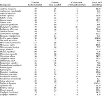
Only the 39 fish species that were well sampled and comprised at least five species of gastrointestinal helminths are included in the present analyses (see table 1). The mean number of individual fish examined per host species ranged from 29 to 162 (mean = 63.9). The basic measures obtained for each component community were: (1) species richness, or the number of species occurring in the community; (2) mean total abundance, or the mean number of individual parasites of all species combined per individual fish; (3) the taxonomic identity of the dominant species, i.e. whether the most abundant species in a component community was a trematode, cestode, nematode or acanthocephalan; and (4) the index of interactivity, CC 50, taken from the study of Poulin & Luque (Reference Poulin and Luque2003) on 31 of the 39 fish species investigated here. The index measures what percentage of host individuals in a sample must be examined for 50% of the parasite species in the component community to be found, when host individuals are ranked from most species-poor to most species-rich (for full details see Poulin & Luque, Reference Poulin and Luque2003). The index essentially measures the tendency for different parasite species in a component community to co-occur in the same host individuals, which is a prerequisite for interspecific interactions; it collapses this and other properties thought to be associated with the degree of interspecific interactions into a single number. Low values of CC 50 indicate interactive parasite communities, whereas high values of CC 50 are expected in communities with little interspecific interaction.
Summary data on the 39 gastrointestinal helminth communities from fish.

Species abundance distributions and model fitting
We constructed species abundance distributions by plotting the relative abundance of each species, expressed as a percentage of the total number of individual helminths in the community, against its rank when all species are ranked from most to least abundant. These distributions were then compared with those predicted by six theoretical models: the general lognormal, the canonical lognormal, the geometric series, the broken stick, the Zipf–Mandelbrot, and the fractal succession model. These are explained in the Appendix.
We fitted the observed rank–abundance plots to those predicted by each of the six models. The three most widely used methods to test goodness-of-fit are based on the log-likelihood ratio, the χ2 and the Kolmogorov–Smirnov distances (Zar, Reference Zar1999). In ecology, abundances are continuous data and the unit chosen influences the three criteria and the test results. Thus, we test the goodness-of-fit on relative abundance data (percentage of total abundance) in our study. With relative data, the χ2 and the log-likelihood ratio could give too much importance to rare species (Tokeshi, Reference Tokeshi1993) so we chose the test associated with the Kolmogorov–Smirnov distances. This test appears to be the most appropriate for fitting mathematical models to relative abundance distributions (Tokeshi, Reference Tokeshi1993; Mouillot et al., Reference Mouillot, Leprêtre, Andrei-Ruiz and Viale2000).
Index of dominance
Because the statistical power of the model fitting procedure is limited by the relatively low species richness of the communities we investigated (compared to the species richness values of communities of free-living organisms), we used a simple index of dominance to assess the magnitude of the numerical supremacy of the top-ranked species in a community. We used the ratio between the overall abundances of those two most common species in each component community, an index hereafter referred to as 1:2 ratio. These abundance ratios are always greater than 1 and increase as the difference in abundance between the most and second most abundant species increases. For each community, we also computed the abundance ratio between the most and third most abundant species (1:3 ratio), because in some communities it appeared that there were two very abundant species and that the drop in abundance only manifested itself beginning with the third-ranked species.
We searched for correlations between the 1:2 ratio or the 1:3 ratio and the species richness and mean total abundance of the community, across all 39 communities, and between the ratios and the index CC 50 across the 31 communities for which index values are available. We also compared the 1:2 ratios and 1:3 ratios between communities in which the dominant species belonged to different taxa, to see if certain taxonomic groups are more likely to achieve numerical dominance in a community. All continuous variables except the CC 50 index were log-transformed prior to these and other analyses, to meet the assumptions of parametric tests.
Results
Across the 39 component communities of gastrointestinal helminths studied here, there was much variation in species richness and mean total abundance (table 1): species richness ranged from 5 to 22 (mean = 8.2), and mean total abundance ranged from 0.75 to 1067 (mean = 47.2). The numerically dominant species was a trematode in 28 communities, a cestode in five communities, a nematode in five communities, and an acanthocephalan in one community.
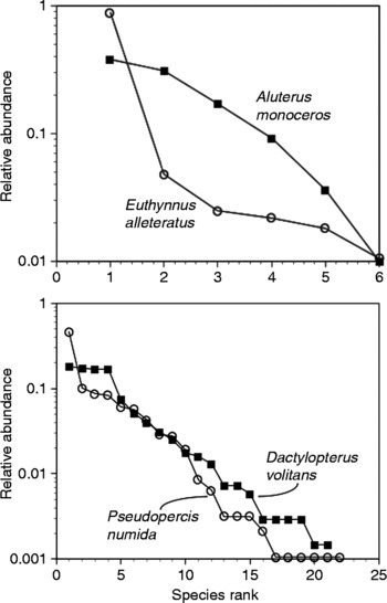
The abundance-versus-rank plots took a variety of shapes (fig. 1). In some communities, there was a sharp drop in abundance, even on a log-scale, from the first- to the second-ranked species, whereas in other communities, the decrease in abundance as a function of rank was gentler among the highly ranked species. The full range of shapes was seen among communities poor in species as well as among species-rich communities (fig. 1).
Species abundance distributions for intestinal helminth communities in four fish species. Two fish species have species-poor helminth communities (top), and two have species-rich communities (bottom). Relative abundance is the percentage of the total number of helminths found in one community that belong to a particular species; note that it is shown on a log-scale. Helminth species are ranked from most to least abundant on the x-axis.

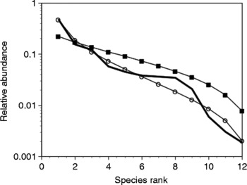
The goodness-of-fit tests comparing the observed abundance distributions to those predicted by the six models considered, however, did not provide conclusive results. Of the six models, only one, the canonical lognormal, was rejected for some communities, but only for five of them (Dactylopterus volitans, Pinguipes brasilianus, Pseudopercis numida, P. semifasciata, and Urophycis brasiliensis). In other words, the abundance-versus-rank curves predicted by five of the models, although quite different from each other in shape and steepness, all provided a fit to the observed data too good to be reliably ascribed to chance; the sixth model performed almost equally well, since its predictions were also too close to observed values (in 34 out of 39 communities) to be dismissed as the product of chance. In many cases, although the output from the models fell close to the observed values, the general shape of the observed and predicted curves showed very little congruence (see example in fig. 2). Given that many communities have relatively low species richness, and that the goodness-of-fit procedure used to test for goodness-of-fit between observed and predicted values is very sensitive to the number of ranks, this may simply be due to a lack of statistical power. I ndeed, there was a significant difference (one-way ANOVA, F 1,37 = 47.87, P < 0.0001) in species richness between the five communities for which the canonical lognormal model could be rejected (mean ± SD, 17.2 ± 5.3) and the remaining communities (6.9 ± 1.9). These two groups of communities did not differ with respect to mean total abundance (F 1,37 = 0.006, P = 0.941). If rejection of a theoretical model is only possible when species richness is very high, we need another way of assessing patterns of numerical dominance in these helminth communities.
Species abundance distributions for intestinal helminth communities in the host fish Mugil platanus. Relative abundance is the percentage of the total number of helminths found in one community that belong to a particular species; note that it is shown on a log-scale. Helminth species are ranked from most to least abundant on the x-axis. The thick line represents the observed abundance distributions, whereas the other lines represent the abundance distributions predicted by either the broken stick model (black squares) or the general lognormal model (open circles).

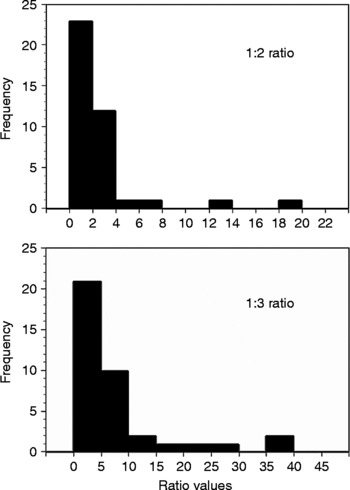
The 1:2 ratios and 1:3 ratios can be used as alternative methods to assess the magnitude of the numerical supremacy of the top-ranked species in a community. The frequency distributions of these ratios across all 39 communities are highly right-skewed, i.e. most values tend toward the lower end of the spectrum (fig. 3). Values for the 1:2 ratio ranged from 1.0 to 18.2, with a geometric mean ± SD (calculated from log-transformed data to account for the skewed distribution) of 2.02 ± 1.97. For the 1:3 ratio, values ranged from 1.1 to 291.5 (this was an outlier corresponding to the community in the fish Trichiurus lepturus), with a geometric mean ± SD of 5.28 ± 3.08. Therefore, in a typical community, the dominant species is twice as abundant as the second most common species, and over five times more abundant than the third most common species. The 1:2 ratio and the 1:3 ratio are obviously correlated with each other (r 2 = 0.368, P = 0.0001), but still capture a slightly different aspect of the abundance distribution.
Frequency distributions of ratio values, for both the abundance ratio between the most and second most abundant species (1 : 2 ratio), and the abundance ratio between the most and third most abundant species (1 : 3 ratio), in 39 component communities of intestinal helminth parasites in marine fishes. One extreme value (291.5) is not shown for the 1 : 3 ratio.

How do the 1:2 ratio and the 1:3 ratio covary with species richness and mean total abundance? Across the 39 communities, the number of individual fish examined per host species did not correlate with either species richness (r 2 = 0.065, P = 0.118) or mean total abundance (r 2 = 0.041, P = 0.220), ruling out any potential effect of sampling biases. There was also no relationship between species richness and mean total abundance (r 2 = 0.002, P = 0.859), and thus the two parameters represent distinct properties of communities. The 1:2 ratio did not correlate with species richness (r 2 = 0.007, P = 0.619) or mean total abundance (r 2 = 0.054, P = 0.156) across all 39 communities. Similarly, the 1:3 ratio did not correlate with species richness (r 2 = 0.038, P = 0.232) or mean total abundance (r 2 = 0.061, P = 0.134) across 38 communities following the exclusion of the outlier community in T. lepturus. There were also no differences in 1:2 ratio or 1:3 ratio between communities dominated by either a trematode, a nematode or a cestode (ANOVAs, both P>0.18).
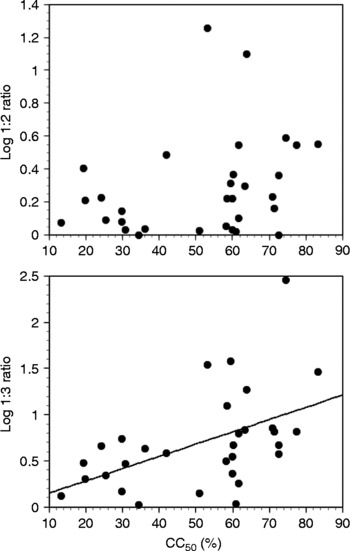
The index CC 50 did not correlate with either species richness or mean total abundance (both P>0.26) across the 31 communities for which data were available. Its values ranged from 13.3 to 83.3%, and thus covered most of the range of possible interactivity. The index CC 50 did not correlate with the 1:2 ratio (r 2 = 0.089, P = 0.103), but there was a positive relationship between the index CC 50 and the 1:3 ratio (r 2 = 0.248, P = 0.0044; see fig. 4). In other words, the difference in relative abundance between the dominant and third most abundant species was greater in communities characterized by weak interspecific interactions.
Relationship between either the abundance ratio between the most and second most abundant species (1:2 ratio), or the abundance ratio between the most and third most abundant species (1:3 ratio), and the interactivity index CC 50, across 31 component communities of intestinal helminth parasites in marine fishes. See the text for details about the index CC 50. The line represents that derived from a linear regression.

Discussion
In both communities of free-living and parasitic organisms, different species occur at vastly different abundances, providing a challenging puzzle for ecologists and parasitologists (McGill et al., Reference McGill, Etienne, Gray, Alonso, Anderson, Benecha, Dornelas, Enquist, Green, He, Hurlbert, Magurran, Marquet, Maurer, Ostling, Soykan, Ugland and White2007; Poulin, Reference Poulin2007). Here, we observed a wide range of species abundance distributions among 39 gastrointestinal helminth communities in fish, with abundance-versus-rank plots showing anywhere from a very steep to a rather gentle drop in abundance between the most abundant species and the next most abundant one. We cannot reject with confidence any of the six theoretical models tested, since the communities are generally too poor in species to allow robust statistical evaluation of the goodness-of-fit between the models' predictions and the observed data. Although the ratio in abundance between the most and the second or third most abundant species in a community varied substantially, these were not correlated either with species richness or the mean number of parasite individuals per host, nor were they influenced by the taxonomic identity of the dominant species. However, the ratio in abundance between the most and the third most abundant species in a community was lower in communities characterized by strong interspecific interactions.
The most common method to compare the relative abundance of different species in natural communities is to plot species abundance distributions (May, Reference May, Cody and Diamond1975; Gaston & Blackburn, Reference Gaston and Blackburn2000; Gray et al., Reference Gray, Bjorgesaeter and Ugland2006; McGill et al., Reference McGill, Etienne, Gray, Alonso, Anderson, Benecha, Dornelas, Enquist, Green, He, Hurlbert, Magurran, Marquet, Maurer, Ostling, Soykan, Ugland and White2007). When comparing observed patterns with those predicted by theoretical models, visual inspection of the plots remains the best method to evaluate similarities or discrepancies (McGill et al., Reference McGill, Etienne, Gray, Alonso, Anderson, Benecha, Dornelas, Enquist, Green, He, Hurlbert, Magurran, Marquet, Maurer, Ostling, Soykan, Ugland and White2007). Here, we have used a much more rigorous method based on a Kolmogorov–Smirnov goodness-of-fit test, although its power was limited by the number of ranks within communities, i.e. by species richness. The only model rejected in some communities was the canonical lognormal model; this is a purely statistical model that makes no biological assumptions but generally provides a good fit to abundance patterns in many types of communities (see McGill et al., Reference McGill, Etienne, Gray, Alonso, Anderson, Benecha, Dornelas, Enquist, Green, He, Hurlbert, Magurran, Marquet, Maurer, Ostling, Soykan, Ugland and White2007). The six models considered here are among the most widely used, the most biologically relevant, and/or the ones usually providing a good fit to empirical data; other models would not shed any new or useful light on parasite species distributions. For example, neutral models based on dispersal processes and equivalence between different species (e.g. Hubbell, Reference Hubbell2001) make assumptions that are clearly invalid in the context of parasite communities (Poulin, Reference Poulin2004).
All else being equal, the total numbers of species or individuals in a community are likely to influence the strength of interspecific interactions, and thus they may affect the shape of species abundance distributions. An earlier study had indeed reported that evenness in abundance among helminth species in the same community was affected by either species richness or mean total parasite abundance (Poulin, Reference Poulin1996). Here, we found no relationships between the ratio in abundance between the most and the second or third most abundant species in a community and either species richness or the mean number of parasites per fish. However, we found that the ratio in abundance between the most and the third most abundant species in a community was significantly related to a more direct measure of interspecific interactions, the index CC 50 of Poulin & Luque (Reference Poulin and Luque2003). According to this index, the difference in relative abundance between the dominant and third most abundant species was lower in communities characterized by strong interspecific interactions, and intensified in non-interactive communities. This finding suggests that strong interactions among helminth species serve to minimize the relative differences in abundance among species, possibly by creating feedback mechanisms through which the abundance of one species is kept in check by other species. In the absence of strong interactions, it may be possible for a few species to achieve marked numerical dominance solely because of their high recruitment rates.
Differences in body size among helminth species in the same community could also explain why certain species become so abundant relative to others (Loehle, Reference Loehle2006). In the majority of animal taxa, the most important correlate of abundance is body size. Among species in a community, abundance almost invariably decreases as body size increases, such that small-bodied species occur at higher densities than larger species (Damuth, Reference Damuth1981; Marquet et al., Reference Marquet, Navarette and Castilla1990; Blackburn & Gaston, Reference Blackburn and Gaston1997; Gaston & Blackburn, Reference Gaston and Blackburn2000). This relationship is one of the most robust known patterns in macroecology; it has been reported for communities involving all kinds of taxa, including parasite communities (Arneberg et al., Reference Arneberg, Skorping and Read1998; but see Poulin, Reference Poulin1999 for exceptions). Given that species belonging to certain taxa, such as cestodes, are generally larger than those of other taxa, such as trematodes, we might expect that the taxonomic identity of the most abundant species could influence the magnitude of its numerical dominance. This was not the case in the present study, with no difference seen in the 1:2 or 1:3 ratios of communities dominated by species of different taxa. There are biological differences other than body size between different helminth taxa that could obscure any size effect. Recently, Poulin & Justine (Reference Poulin and Justine2008) have looked for a relation between size differences and abundance ratios among ectoparasitic monogenean species belonging to the same family and found on reef fishes of New Caledonia. They found that the huge differences in abundance observed among co-occurring species had nothing to do with differences in their body size. It thus appears that body size differences cannot provide a simple explanation for patterns of species abundance distributions in parasite communities.
Interspecific interactions seem capable of affecting the magnitude of the gap in abundance between the most abundant species in a parasite community, and may thus influence the overall shape of species abundance distributions. Clearly, however, other processes must be at work to account for the wide variation in the form of abundance-versus-rank plots seen among the fish parasite communities studied here. As a next step, it will be interesting, though challenging, to see whether parameters associated with recruitment rates can explain observed patterns of relative abundances independently of interspecific interactions.
Acknowledgements
J.L.L. was supported by a Research Fellowship from CNPq (Conselho Nacional de Desenvolvimento Científico e Tecnológico, Brazil) and by grants from FAPERJ (Fundação de Amparo à Pesquisa do Estado do Rio de Janeiro).
Appendix
Six theoretical models of relative species abundance were tested in this study. Following Tokeshi (Reference Tokeshi1999), the first two are considered statistically oriented models; the next two, niche-oriented models; and the last two, fractal-oriented models. The six models are:
General lognormal
In a productive community, the abundance distribution of species is often lognormal (Preston, Reference Preston1948). This is clearly a statistical model, because it is not based on any ecological hypothesis. Nevertheless, several authors have proposed ecological explanations for this kind of distribution in ecological communities (see May, Reference May, Cody and Diamond1975). For instance, Sugihara (Reference Sugihara1980) argued that a sequential division of the ecological niche along several axes leads to a general lognormal distribution in species abundances. In the model derived for rank-abundance plots (Frontier, Reference Frontier1985; Wilson, Reference Wilson1991), the abundance of species i is:

where S is the number of species,  the average logarithm of abundances and ϕ− 1 the inverse cumulative distribution function of a normal distribution. This model has two optimized parameters, σ and
 (Frontier, Reference Frontier1985; Wilson, Reference Wilson1991). For frequency instead of abundance we get:

Here we have one fixed parameter which is the number of species, and two optimized parameters which are the mean and the standard deviation of log frequencies ( and σ).
Canonical lognormal
The canonical lognormal is a particular case of the general lognormal in the sense that the standard deviation of log abundances (σ) is proportional to the number of species (S) (May, Reference May, Cody and Diamond1975) as:

Thus, this model has one parameter less than the general lognormal (Wilson, Reference Wilson1991). As for the general lognormal, there is no ecological basis for this model and, moreover, May (Reference May, Cody and Diamond1975) claimed that the canonical lognormal distribution was only an artefact due to the general lognormal curve and regression techniques. Nevertheless, Sugihara (Reference Sugihara1980) showed that a minimal form of community organization involving hierarchically related niches can explain the canonical lognormal distribution, which has been observed for various communities ranging from diatoms to soil arthropods. In this model, the frequency F i of species i is:

where  , the mean of log frequencies, is the only optimized parameter (Wilson, Reference Wilson1991).
Geometric series
This model, the oldest one for rank-abundance distributions, is also called the niche pre-emption model. Although introduced in a statistical form by Motomura (Reference Motomura1947), this model is now classified in the niche-oriented category because it suggests that each new species in the community apportions a fraction t of the remaining resources with its abundance being proportional to this fraction (Whittaker, Reference Whittaker1965; Tokeshi, Reference Tokeshi1999). Thus with A 1 being the abundance of the first species, we obtain for the abundance of species with rank i:

In a log–linear rank–abundance plot, this model is a straight line following the equation:

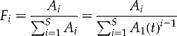
This model is clearly a two–parameter model and the parameters (A 1 and t) can be estimated by classical linear regression (Wilson, Reference Wilson1991), but if we consider the frequency (F i for species i) instead of abundance, to avoid problems with abundance metrics, we have with S species:
and
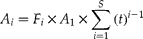
Then the log linear model is:
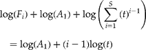
We obtain finally:

This model has only one parameter (t) and cannot be fitted with linear methods. However, with a Monte-Carlo optimization method, we can estimate t.
Broken stick
This model, first proposed by MacArthur (Reference MacArthur1957), suggests that abundances reflect the resources that each species apportions along a one–dimensional gradient. It assumes that the total resource space is filled by species, that there is no overlap between niches, and that resources are apportioned at random with no competition (Legendre & Legendre, Reference Legendre and Legendre1998). This model can be expressed as:

with S species and A i being the abundance of species i. This model has originally only one parameter: the mean abundance  (Wilson, Reference Wilson1991). If we consider species frequencies we have:
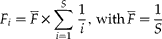
Thus the model for the frequency of species i (F i) is:

This model has no optimized parameter, and for any given number of species (fixed parameter) the broken stick theoretical frequencies are perfectly known. This model does not require optimization procedures.
Zipf–Mandelbrot
A recent deterministic model applied in ecology (Frontier, Reference Frontier1985) is the Zipf–Mandelbrot model, which was initially developed for linguistic or socio-economic studies (Zipf, Reference Zipf1965; Mandelbrot, Reference Mandelbrot1977, Reference Mandelbrot1982). In this model, the frequency F i of a species of rank i is as follows:

with:

S is the number of species present and the parameters β and γ have an ecological interpretation: β represents the diversity of the environment, i.e. the niche diversity, and γ the predictability of the ecosystem, i.e. the average probability of the appearance of a species (Frontier, Reference Frontier1985; Wilson, Reference Wilson1991). The underlying hypotheses of this parametric model are thus relevant from an ecological point of view, as has been confirmed in several studies (e.g. Aoki, Reference Aoki1995; Wilson & Gitay, Reference Wilson and Gitay1995). However, a major problem with the use of this model comes from the strong correlation existing between β and γ, the model's two parameters (Mouillot et al., Reference Mouillot, Leprêtre, Andrei-Ruiz and Viale2000). Optimization thus becomes difficult and the model parameter estimates lack robustness (Mouillot et al., Reference Mouillot, Leprêtre, Andrei-Ruiz and Viale2000). Indeed, researchers who have used the Zipf–Mandelbrot model all observed a lack of convergence of their optimization algorithms (Wilson, Reference Wilson1991; Aoki, Reference Aoki1995). Here, we focus only on the simplified form of the Zipf–Mandelbrot model; with β = 0 we have the Zipf model for the frequency of species i:

with γ being the only parameter of the model and 1/γ assumed to be a fractal dimension (Mandelbrot, Reference Mandelbrot1977, Reference Mandelbrot1982; Frontier, Reference Frontier1985). Thus, the relative abundance of S successive species of rank i are ruled by a self-similar process and the parameter γ. When γ is high, the slope of the dominance–diversity curve on a log–log graph is very steep and the decrease in species frequency very pronounced.
Fractal succession
To describe ecological successions, Frontier (Reference Frontier and Novak1994) proposed a theory for biomass partitioning among successive species, arguing that at each step of the succession, K new species appear which are k times less abundant. This self-similar process through time is a fractal process to describe species accumulation with K = k d and d being a fractal dimension. Frontier (Reference Frontier and Novak1994) also demonstrated the relationship existing between the parameter d and the parameter γ of the Zipf model described above with d = 1/γ. Based on this theory, Mouillot et al. (Reference Mouillot, Leprêtre, Andrei-Ruiz and Viale2000) proposed a fractal model for relative abundance distribution of species through a species accumulation process. This fractal succession model has one fixed parameter which is the number of species and two optimized parameters: K (the number of new species in the community) and k (the factor for dividing abundance for the new species).