2 Flow cases and numerical method

Table 1.

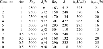
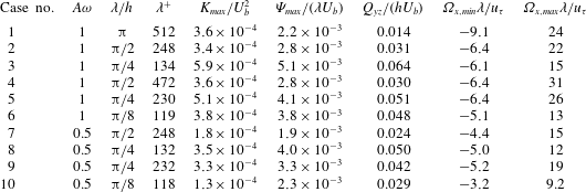
Summary of simulation parameters for the various cases, where $Re_{h}=hU_{b}/\unicode[STIX]{x1D708}$ , $\unicode[STIX]{x1D706}/h=2\unicode[STIX]{x03C0}/(\unicode[STIX]{x1D714}h)$ , $Re_{\unicode[STIX]{x1D70F}}=hu_{\unicode[STIX]{x1D70F}}/\unicode[STIX]{x1D708}$ and $\unicode[STIX]{x1D706}^{+}=\unicode[STIX]{x1D706}u_{\unicode[STIX]{x1D70F}}/\unicode[STIX]{x1D708}$ . The averaging time considered to obtain turbulence statistics is given by $t_{a}$ .

The geometry of the walls is defined in (2.1), where $A$ and $\unicode[STIX]{x1D714}$ are the wave amplitude and frequency, respectively. The upper and lower walls are in phase such that the half-height of the channel $h$ is uniform in the spanwise direction. The flow is fully developed in the homogeneous streamwise direction, where periodic boundary conditions are specified. The periodicity of the walls enables the use of periodic boundary conditions also in the inhomogeneous spanwise direction. The streamwise and spanwise lengths of the channel are $L_{x}=8.25h$ and $L_{z}=\unicode[STIX]{x03C0}h$ , respectively, where $x/h\in [0,8.25]$ and $z/h\in [-\unicode[STIX]{x03C0}/2,\unicode[STIX]{x03C0}/2]$ . According to Lozano-Durán & Jiménez (Reference Lozano-Durán and Jiménez2014), these sizes are large enough to reproduce the one-point statistics of larger boxes in spanwise-periodic channels with straight walls at $Re_{\unicode[STIX]{x1D70F}}\leqslant 4179$ . The sinusoidal walls introduce a pattern of internal and external streamwise corners with different angles and sizes. The angle of the corner is determined by the product $A\unicode[STIX]{x1D714}$ such that $\unicode[STIX]{x03C0}-2\arctan (A\unicode[STIX]{x1D714})$ is the angle of the concave corner (valley) and $\unicode[STIX]{x03C0}+2\arctan (A\unicode[STIX]{x1D714})$ is the angle of the convex one (peak). An interesting property of this parameter is that it determines the curvilinear length of the wall $L_{c}$ , which is defined in (2.2). Therefore, the wall surface of the channels only depends on the angle of the corner. Decreasing the amplitude of the wave is compensated by an increased number of corners at constant $A\unicode[STIX]{x1D714}$ . In other words, a segment of length $L_{c}$ can be folded to create any integer number of corners of the corresponding size, which is determined by the angle $A\unicode[STIX]{x1D714}$ , between $z/h=-\unicode[STIX]{x03C0}/2$ and $z/h=\unicode[STIX]{x03C0}/2$ . The size of the corner is associated with the wavelength of the wall, which is defined using outer and inner scaling as $\unicode[STIX]{x1D706}/h=2\unicode[STIX]{x03C0}/(\unicode[STIX]{x1D714}h)$ and $\unicode[STIX]{x1D706}^{+}=2\unicode[STIX]{x03C0}u_{\unicode[STIX]{x1D70F}}/(\unicode[STIX]{x1D714}\unicode[STIX]{x1D708})$ , respectively. The various cases under study are summarized in table 1.

(2.1) $$\begin{eqnarray}\displaystyle & y_{w}=\pm h+A\cos (\unicode[STIX]{x1D714}z), & \displaystyle\end{eqnarray}$$

(2.2) $$\begin{eqnarray}\displaystyle & \displaystyle L_{c}=\int _{-\unicode[STIX]{x03C0}/2}^{\unicode[STIX]{x03C0}/2}\sqrt{1+\left(\frac{\text{d}y_{w}}{\text{d}z}\right)^{2}}\,\text{d}z. & \displaystyle\end{eqnarray}$$

The DNSs were performed using the open-source numerical code Nek5000, developed by Fischer, Lottes & Kerkemeier (Reference Fischer, Lottes and Kerkemeier2008) at the Argonne National Laboratory. The code is based on the spectral-element method (SEM), originally proposed by Patera (Reference Patera1984), and employs Gauss–Lobatto–Legendre points for the orthogonal collocation. Third-order discretization in time is used with explicit extrapolation and implicit backward differentiation for the nonlinear and viscous terms, respectively. The constant time step is chosen to prevent the maximum Courant numbers from exceeding the value of 0.35. In all the cases under consideration we use a polynomial order of $N=11$ to express the velocity within each element, and $N=9$ is considered for the pressure (Maday & Patera Reference Maday, Patera and Noor1989). The size of the elements is adjusted to satisfy the standard resolution criteria for DNS with at least three and fourteen grid points located below $y^{+}=1$ and 10, respectively, where the superscript ‘ $+$ ’ denotes inner scaling in terms of $u_{\unicode[STIX]{x1D70F}}$ or the viscous length $\unicode[STIX]{x1D708}/u_{\unicode[STIX]{x1D70F}}$ . In the core of the channel, the maximum and minimum spacing in viscous units between the spectral nodes of the largest elements is $\unicode[STIX]{x0394}x^{+}\simeq (2,10)$ in the streamwise direction and $\unicode[STIX]{x0394}y,z^{+}\simeq (1,5)$ in the vertical/spanwise directions. 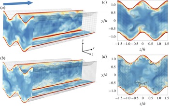The resulting number of grid points is 7 and 43 million for the cases with $Re_{h}=2500$ and 5000, respectively. The computational meshes corresponding to cases 2 and 4 are shown in figure 1. The instantaneous velocity field is shown at the inlet plane $x/h=0$ , the centre of the channel $z/h=0$ and the plane tangential to the peaks of the lower wall at $y/h=-0.75$ . The cross-sectional distribution of the instantaneous cross-flow at $x/h=0$ is shown in the panels on the right-hand side of the figure. Note that ejections can be identified as red filaments of low-momentum fluid convected out of the wall towards the core of the channel by the instantaneous cross-flow. The figure shows that ejections are preferentially located and concentrated near the peaks, tilting towards the vertical direction. The figure shows several ejections concentrated near the peaks and tilting towards the vertical direction. In § 5 we show that this is, in fact, the preferential behaviour of this type of event. The number of ejections per wavelength roughly doubles from $Re_{h}=2500$ to 5000 and their averaged outer-scaled size and spacing are halved with respect to the size of the corners.

Figure 1.

(a,b) Distribution of the computational mesh and the instantaneous streamwise velocity in planes $x/h=0$ , $z/h=0$ and $y/h=-0.75$ corresponding to cases 2 (a,c) and 4 (b,d) defined in table 1. The arrow indicates the flow direction; red and blue denote low and high velocity, respectively. (c,d) Cross-sectional distribution of the instantaneous cross-flow.

The flow is initially laminar and turbulence is triggered using a volume-force tripping method; see Schlatter & Örlü (Reference Schlatter and Örlü2012) and Hosseini et al. (Reference Hosseini, Vinuesa, Schlatter, Hanifi and Henningson2016). Once the flow becomes fully turbulent, after roughly 25 convective time units, the tripping is disconnected and the polynomial order is raised from $N=5$ to $N=7$ for another 25 convective units; finally, the polynomial order is increased to $N=11$ . The issues of initial transient identification and required averaging times are discussed by Vinuesa et al. (Reference Vinuesa, Prus, Schlatter and Nagib2016) for the turbulent channel and duct flows. A total of 71 quantities are computed by averaging in time and in the streamwise direction in order to obtain turbulence statistics. The averaging times are shown in table 1, expressed in convective time units $(t_{a}U_{b}/h)$ and eddy-turnover times $(t_{a}u_{\unicode[STIX]{x1D70F}}/h)$ . Unlike the spanwise-periodic channel with flat walls, the turbulence statistics cannot be averaged in the spanwise inhomogeneous direction. However, the periodic geometry of the wall is utilized to increase the effective averaging time, a fact that raises the number of samples by a factor of $2\unicode[STIX]{x1D714}h$ . Therefore, shorter averaging periods are required to obtain converged statistics in the channels with larger $\unicode[STIX]{x1D714}h$ values. 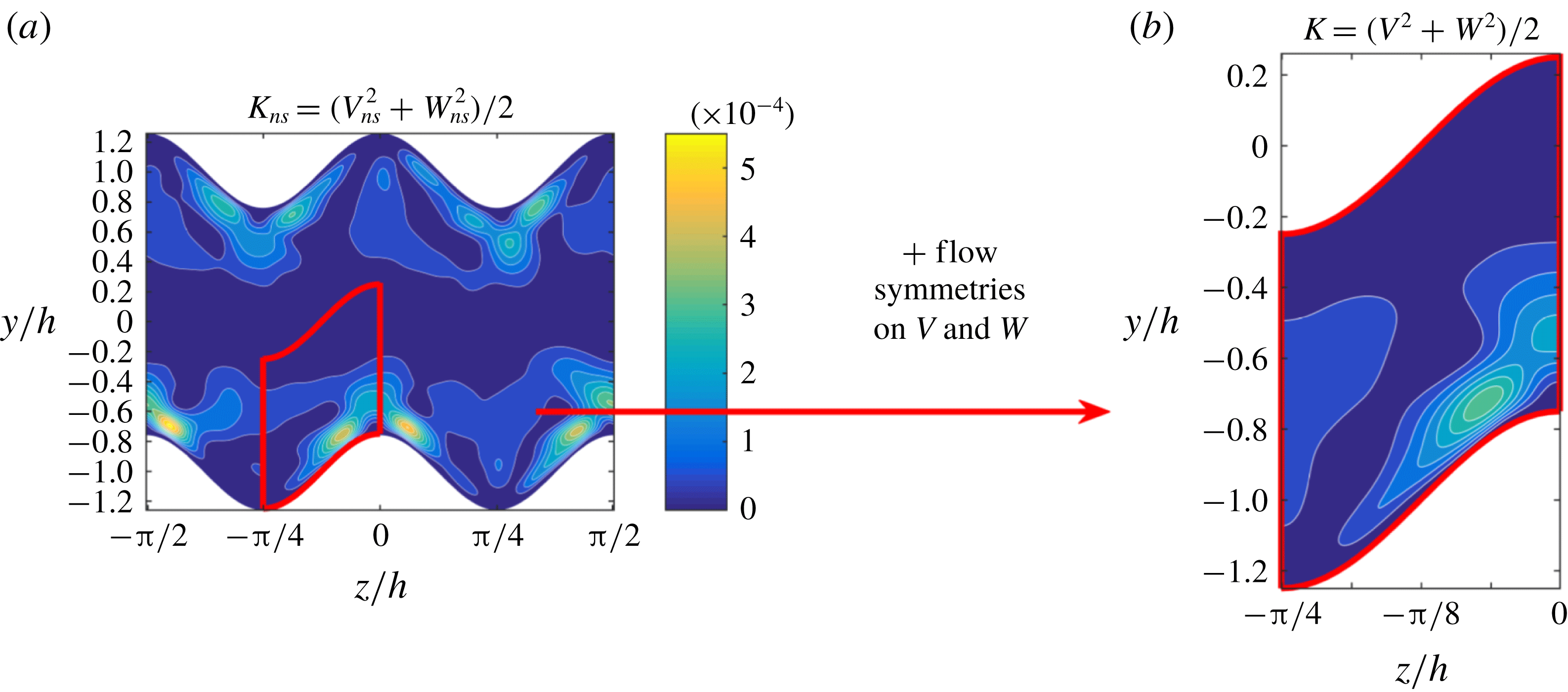The kinetic energy of the mean cross-flow $K=(V^{2}+W^{2})/2$ (Vinuesa, Schlatter & Nagib Reference Vinuesa, Schlatter and Nagib2018) is shown in figure 2 before (a) and after (b) using the flow symmetries on the streamwise and time-averaged cross-flow components. In the present study we denote the kinetic energy of secondary flow before and after applying the flow symmetries as $K_{ns}$ and $K$ , respectively. Since the instantaneous velocity field, shown in figure 1, is not periodic in the spanwise direction, $K_{ns}(t_{a})$ will only be periodic in this direction when averaged for long periods of time $t_{a}$ . Note that the converged statistics in the entire domain can be reconstructed from the solution in the red window of this figure.

Figure 2.

Kinetic energy of the mean cross-flow corresponding to case 2. The subscript ‘ $ns$ ’ denotes the fact that the velocity components $V_{ns}$ and $W_{ns}$ were only averaged in time and in the streamwise direction.

3 Mean cross-flow characterization

As expected, the mean cross-flow behaviour in the valleys and peaks of the wall is analogous to the one found in the internal corner by Gavrilakis (Reference Gavrilakis1992) and the external corner by Moinuddin et al. (Reference Moinuddin, Joubert and Chong2004), respectively. The alternating pattern of valleys and peaks leads to an interaction between the streamwise vortices associated with each type of corner, a fact that enhances the secondary flow. Consequently, the mean cross-flow is always directed from the core of the channel to the valleys, concentrating in the buffer-layer region and returning to the core through the peaks. Interestingly, in some cases this interaction is also present between peaks and valleys located in opposite walls. 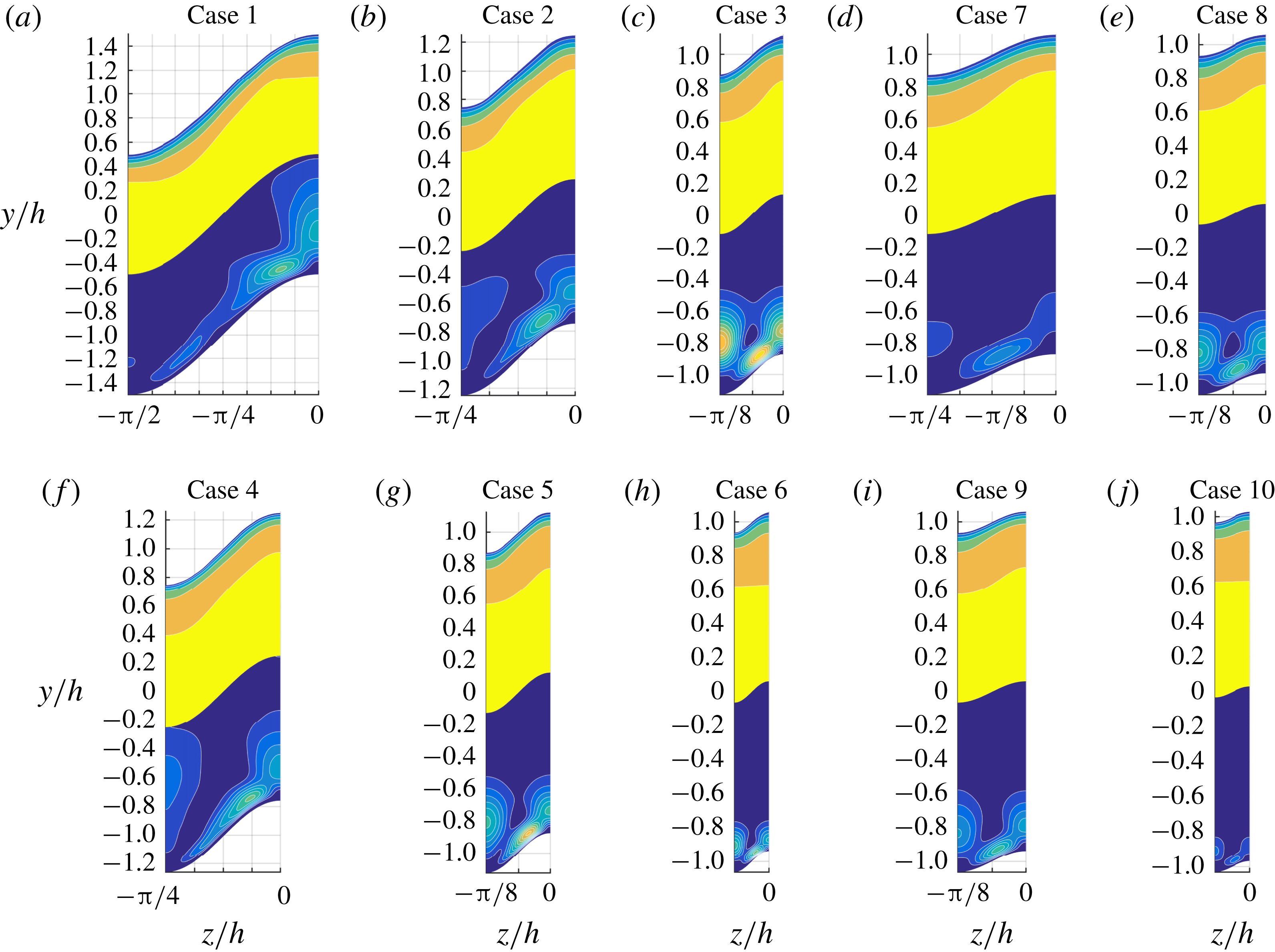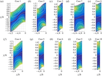Similarly, the various combinations of wavelengths $\unicode[STIX]{x1D706}$ and corner angles $A\unicode[STIX]{x1D714}$ lead to qualitatively and quantitatively different cross-flow and streamwise velocity distributions, as shown in figures 3 and 4 for half a wavelength. Note that the distributions shown in figures 3 and 4 are symmetric and antisymmetric with respect to the $z/h=0$ and $z/h=-\unicode[STIX]{x1D706}/2$ planes, respectively. The cross-sectional distributions of $K$ and the streamwise velocity $U$ are shown in figure 3, scaled with $U_{b}$ . Another alternative to scale $K$ is to use the mean kinetic energy of the instantaneous cross-flow $k$ , which is defined in (3.1). The ratio $K/k$ represents the relative amount of the kinetic energy of the instantaneous cross-flow that is converted into kinetic energy of the mean cross-flow, thus $K/k\leqslant 1$ and its highest value over all the cases is $K/k=0.45$ , corresponding to case 3. Finally, the streamfunction of the mean cross-flow $\unicode[STIX]{x1D6F9}$ and the streamwise vorticity $\unicode[STIX]{x1D6FA}_{x}$ are shown in figure 4 for the various cases under study. Note that the magnitude and distribution of both quantities mainly depend on the wavelength $\unicode[STIX]{x1D706}$ .

(3.1) $$\begin{eqnarray}k=\frac{\overline{v^{2}+w^{2}}}{2}=\frac{\overline{v^{2}}+\overline{w^{2}}}{2}.\end{eqnarray}$$

Figure 3.

(Top half of each panel) Streamwise velocity $U/U_{b}$ (6 contours every 0.2). (Bottom half of each panel) kinetic energy of the mean cross-flow $K/U_{b}^{2}$ (13 contours every $5\times 10^{-5}$ ). The number of each case is indicated in the corresponding panels. Panels (a–e) and (f–j) correspond to cases at $Re_{h}=2500$ and 5000, respectively. The background grid has spanwise and vertical spacing of $\unicode[STIX]{x03C0}/16$ and 0.2, respectively. All the distributions are symmetric with respect to the $z/h=0$ and $z/h=-\unicode[STIX]{x1D706}/2$ planes.

Figure 4.

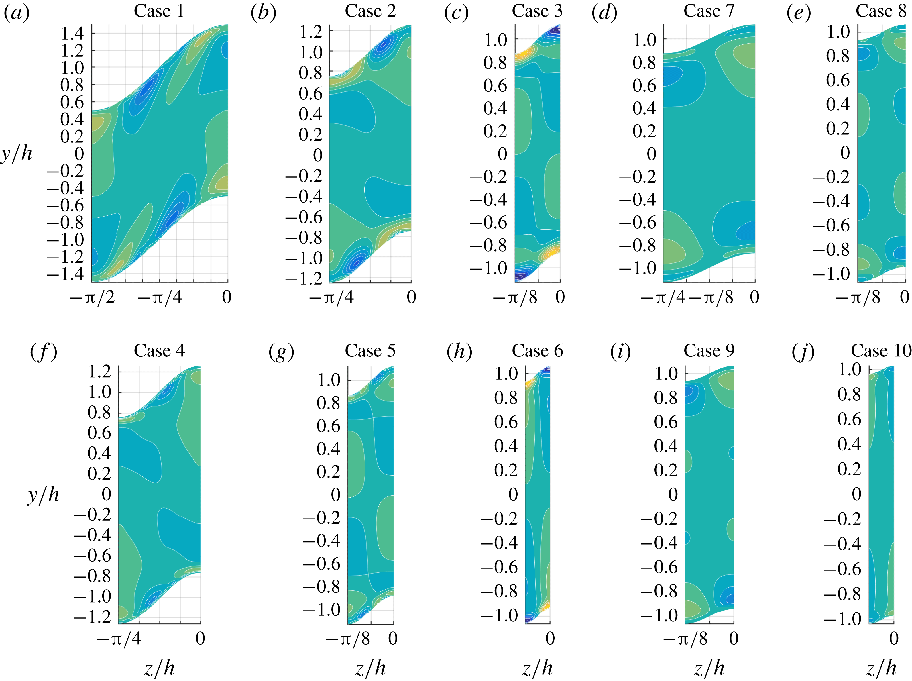
(Black lines on all panels) Distribution of the mean cross-flow streamfunction $\unicode[STIX]{x1D6F9}/(hU_{b})$ (14 red contours every $0.5\times 10^{-3}$ ). Distribution of the mean streamwise vorticity $\unicode[STIX]{x1D6FA}_{x}\unicode[STIX]{x1D708}/{u_{\unicode[STIX]{x1D70F}}}^{2}$ (16 coloured contours every 0.01). The number of each case is indicated in the corresponding panels. Panels (a–e) and (f–j) correspond to cases at $Re_{h}=2500$ and 5000, respectively. The background grid has spanwise and vertical spacing of $\unicode[STIX]{x03C0}/16$ and 0.2, respectively. All the distributions are antisymmetric with respect to the $z/h=0$ and $z/h=-\unicode[STIX]{x1D706}/2$ planes.

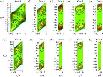
Three qualitatively different $\unicode[STIX]{x1D6F9}$ distributions are observed depending on $\unicode[STIX]{x1D706}/h$ and $A\unicode[STIX]{x1D714}$ . In case 1, which is the case with the highest $\unicode[STIX]{x1D706}/h=\unicode[STIX]{x03C0}$ and $A\unicode[STIX]{x1D714}=1$ values, the secondary flow forms one streamwise vortex per half- $\unicode[STIX]{x1D706}$ which extends throughout the entire cross-section of the channel. The mean cross-flow leaving the near-wall region through the peaks is redirected towards the closest peaks and valleys located in the opposite wall. The maximum value of $\unicode[STIX]{x1D6F9}$ is located at the intersection between the two segments joining together each pair of peaks and valleys. The distributions of $\unicode[STIX]{x1D6F9}$ and $K$ show that the secondary flow accelerates near the peaks and valleys and decelerates everywhere else, including the near-wall region around $y/h\simeq 1$ . The kinetic energy of the mean cross-flow $K$ is much stronger around the external corner, where three local maximum values are located and surrounded by lobe-shaped regions of high- $K$ . In the study by Goldstein & Tuan (Reference Goldstein and Tuan1998), the cross-flow was also found to be stronger near the peaks of the riblets than in the valleys between them. The local maximum of $K$ on the side of the peak is caused by the wall-tangent component of the cross-flow in the buffer layer. The wall-normal derivate of the wall-tangent velocity component in this region is the main contribution to the positive region of streamwise vorticity $\unicode[STIX]{x1D6FA}_{x}>0$ , which is located below the buffer layer near the peak. The negative regions of $\unicode[STIX]{x1D6FA}_{x}$ near the peaks and valleys are associated with the rotation of the streamlines. Namely, the secondary flow approaching the wall through the valleys turns in the wall-tangent direction and, after reaching the peak along the wall, curves into the core of the channel. Note that a local minimum of $\unicode[STIX]{x1D6FA}_{x}<0$ is also present near the valley, where $K$ exhibits three weaker local maximum values.

In cases 2 and 4, the size of the wave is halved with respect to case 1 by reducing the wavelength from $\unicode[STIX]{x03C0}/2$ to $\unicode[STIX]{x03C0}/4$ while maintaining its aspect ratio $A\unicode[STIX]{x1D714}=1$ . Note that both cases exhibit similar distributions of $\unicode[STIX]{x1D6F9}$ despite their different bulk Reynolds numbers and $\unicode[STIX]{x1D706}^{+}$ values, a fact that supports the argument that $\unicode[STIX]{x1D6F9}$ scales in outer units. The instantaneous streamwise and cross-stream velocity distributions corresponding to these cases are shown in figure 1. The secondary flow forms two smaller vortices per half- $\unicode[STIX]{x1D706}$ located near the peaks and with the same rotation directions. The smaller $A/h$ values lead to a reduced interaction between the secondary flow associated with each wall, and less than 25 % of the mean cross-flow rate is recirculated around both of the vortices. Note that the maximum value of the streamfunction of the mean cross-flow $\unicode[STIX]{x1D6F9}_{max}$ corresponds to the total cross-flow rate recirculated around its location. The total cross-flow rate in the channel $Q_{yz}$ is defined in (3.2), where $\unicode[STIX]{x1D6F9}_{rc}$ is the cross-flow rate that is common to two vortices located on the opposite walls and $N_{v\unicode[STIX]{x1D706}}$ is the number of vortices per wavelength, which is 2 in case 1 and 4 in the other cases. As $\unicode[STIX]{x1D706}/h$ is reduced by a factor of 2 from $\unicode[STIX]{x03C0}$ to $\unicode[STIX]{x03C0}/2$ , the total cross-flow rate is increased by the same factor, from around 0.015 in case 1 to 0.03 in cases 2 and 4, due to the addition of more vortices in the spanwise direction. However, the total cross-flow rate per half- $\unicode[STIX]{x1D706}$ is roughly equal, thus the $Q_{yz}$ of the single vortex of case 1 is distributed among the upper and lower vortices of cases 2 and 4. Furthermore, the resulting vortices must rotate faster in order to maintain the total cross-flow rate per half- $\unicode[STIX]{x1D706}$ as $\unicode[STIX]{x1D706}$ is halved. This behaviour is observed in figure 3, where the magnitude of $K$ rises along the centreplane of the valleys and only exhibits one local maximum value on the side of the wave, thus no cross-flow reduction occurs in the $y/h\simeq 1$ region.

(3.2) $$\begin{eqnarray}\frac{Q_{yz}}{hU_{b}}=\frac{\unicode[STIX]{x1D6F9}_{max}-\unicode[STIX]{x1D6F9}_{rc}}{hU_{b}}N_{v\unicode[STIX]{x1D706}}\frac{\unicode[STIX]{x03C0}}{\unicode[STIX]{x1D706}}.\end{eqnarray}$$

A similar effect is observed for smaller values of $\unicode[STIX]{x1D706}/h$ , as can be clearly appreciated as one observes cases 1, 2 and 3; also when one moves from case 4 to 5; and the same is observed when going from case 7 to 8. The dimensions of the high- $K$ lobes shrink with $\unicode[STIX]{x1D706}$ while their magnitude increases. However, the maximum value of the kinetic energy $K_{max}$ is reduced from cases 5 to 6 and 9 to 10. The value of $K/k$ is also reduced indicating that the decline of $K$ is not caused by a lack of instantaneous kinetic energy. Further insight on this non-monotonic behaviour can be gained by considering the inner-scaled wavelength $\unicode[STIX]{x1D706}^{+}$ . Note that in cases 6 and 10, $\unicode[STIX]{x1D706}^{+}<120\simeq 100$ , where 100 is the average spanwise wavelength of the bursting cycle and separation between velocity streaks of the same sign; see Kline et al. (Reference Kline, Reynolds, Schraub and Runstadler1967) and Gupta et al. (Reference Gupta, Laufer and Kaplan1971). This distance was also identified by Jiménez & Moin (Reference Jiménez and Moin1991) as the minimum inner-scaled spanwise width required in turbulent channel flow simulations to prevent relaminarization and reproduce the low-order statistics of experiments. Therefore, the largest high- and low-speed streaks cannot tend to be simultaneously accommodated near valleys and peaks, respectively, as $\unicode[STIX]{x1D706}^{+}/2\simeq 60$ . 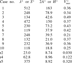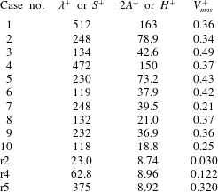In these cases, only the smaller and weaker structures with spanwise lengths $l_{z}^{+}\leqslant 60$ can contribute to the mean cross-flow, a fact that leads to the reduced $K_{max}$ values. The decay of the secondary flow in riblets with decreasing spanwise separation and heights was reported by Goldstein & Tuan (Reference Goldstein and Tuan1998). The authors suggested that if the separation is small the riblets shield each other from the spanwise fluctuations. 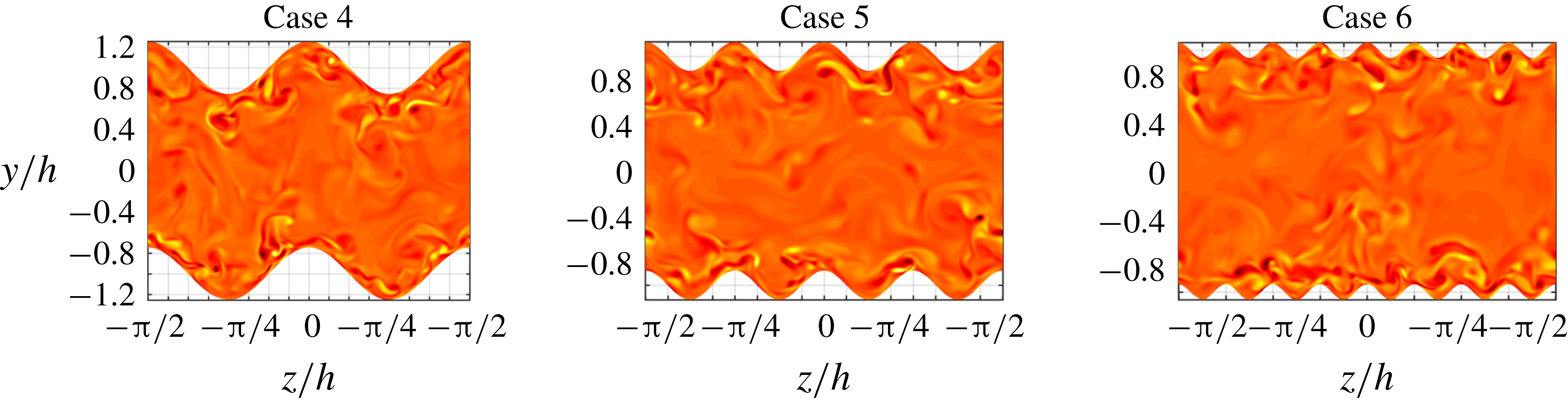In table 2 we compare the inner-scaled mean vertical velocity $V_{max}^{+}$ in the channel with riblets and sinusoidal walls. The results show that cases 6 and 10 are on the verge of this behaviour and highlight the role of inhomogeneously distributed streaks in the production of the secondary flow. This was previously discussed by Pinelli et al. (Reference Pinelli, Uhlmann, Sekimoto and Kawahara2010) in square ducts, Vinuesa et al. (Reference Vinuesa, Noorani, Lozano-Durán, El Khoury, Schlatter, Fischer and Nagib2014) in rectangular ducts, Marin et al. (Reference Marin, Vinuesa, Obabko and Schlatter2016) in hexagonal ducts and Vidal et al. (Reference Vidal, Vinuesa, Schlatter and Nagib2017, Reference Vidal, Vinuesa, Schlatter and Nagib2018) in ducts with rounded corners. Figure 5 shows the instantaneous streamwise vorticity $\unicode[STIX]{x1D714}_{x}$ corresponding to cases 4, 5 and 6 at $Re_{h}=5000$ , with decreasing $\unicode[STIX]{x1D706}^{+}$ . Note the counter-rotating regions of high- $\unicode[STIX]{x1D714}_{x}$ located in the near-wall region. The figure illustrates the fact that the wavelength in case 6 can barely fit two simultaneous counter-rotating streamwise vortices and is not large enough to fit some vortex pairs. Furthermore, if the wavelength is much smaller than the size of the streaks, the geometry of the wall can be considered as spanwise-homogeneous roughness, inhibiting inhomogeneous interaction between bursting events.

Table 2.

Inner-scaled maximum mean vertical velocity $V_{max}^{+}$ in the channel with sinusoidal walls (cases 1–10) and with riblets (r2, r4 and r5), where $S^{+}$ and $H^{+}$ are the spanwise separation and height of the riblets, respectively. The data and case number for the cases with riblets correspond to table 1 in Goldstein & Tuan (Reference Goldstein and Tuan1998).

Figure 5.

Instantaneous streamwise vorticity $\unicode[STIX]{x1D714}_{x}\unicode[STIX]{x1D708}/u_{\unicode[STIX]{x1D70F}}^{2}$ . Dark red and light yellow denote intense negative and positive $\unicode[STIX]{x1D714}_{x}$ , respectively. The number of each case is indicated in the corresponding panels. The background grid has spanwise and vertical spacing of $\unicode[STIX]{x03C0}/16$ and 0.2, respectively.

In square ducts, Pinelli et al. (Reference Pinelli, Uhlmann, Sekimoto and Kawahara2010) found that the outer peak of $\unicode[STIX]{x1D6FA}_{x}$ and the distribution of $\unicode[STIX]{x1D6F9}$ coincide at low Reynolds numbers and gradually separate for increasing $Re$ . The authors conjectured that the secondary flow was the result of the contribution of the different scales of $\unicode[STIX]{x1D714}_{x}$ . They argued that the upper and lower bounds for these scales are the geometry of the duct and the quasi-streamwise vortices associated with the near-wall velocity streaks, respectively. Decreasing the Reynolds number raises the lower bound and reduces the separation between scales. The results with sinusoidal walls show that decreasing $\unicode[STIX]{x1D706}/h$ or $A\unicode[STIX]{x1D714}$ lowers the upper bound and has a similar effect on the $\unicode[STIX]{x1D6FA}_{x}$ and $\unicode[STIX]{x1D6F9}$ distributions, filtering the contribution of the largest scales. Assuming that the secondary flow is determined by the separation between the largest and smallest contributing scales implies that a cross-flow distribution in which the upper bound is determined by the wave parameters can be reproduced at higher Reynolds numbers by adjusting such parameters. 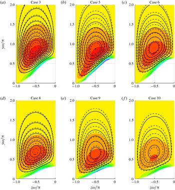In order to assess the validity of this assumption we have analysed the cases where $\unicode[STIX]{x1D706}\ll h$ (cases 3, 5, 6, 7, 8, 9, 10) in further detail. It has been found that the distribution of $\unicode[STIX]{x1D6F9}$ almost entirely depends on $\unicode[STIX]{x1D706}/h$ , whereas the distribution of $\unicode[STIX]{x1D6FA}_{x}$ depends on $\unicode[STIX]{x1D706}^{+}$ , as shown in figure 6. In this figure the vertical and spanwise coordinates are scaled with $\unicode[STIX]{x1D714}=2\unicode[STIX]{x03C0}/\unicode[STIX]{x1D706}$ such that the aspect ratio of the corner is preserved and the results are represented on a common scale from $z\unicode[STIX]{x1D714}/\unicode[STIX]{x03C0}=-1$ to 0. The streamfunction $\unicode[STIX]{x1D6F9}$ is scaled with $\unicode[STIX]{x1D706}$ and both $U_{b}$ and $u_{\unicode[STIX]{x1D70F}}$ , whereas $\unicode[STIX]{x1D6FA}_{x}$ is scaled with $\unicode[STIX]{x1D706}$ and $u_{\unicode[STIX]{x1D70F}}$ . The results show that both quantities depend on $\unicode[STIX]{x1D706}$ instead of $h$ . Note that their distributions are very similar in cases 3–6 and 8–10, where the effect of doubling the Reynolds number is compensated by halving the wavelength; however, their magnitude is reduced. The reduction could be caused by the small inner-scaled wavelength, as mentioned above. Interestingly, the magnitude of $\unicode[STIX]{x1D6F9}$ and of the negative $\unicode[STIX]{x1D6FA}_{x}<0$ , which is located above the buffer layer, are determined by $\unicode[STIX]{x1D706}/h$ . Nevertheless, their distribution depends on $\unicode[STIX]{x1D706}^{+}$ . On the other hand, both the distribution and magnitude of the near-wall region of $\unicode[STIX]{x1D6FA}_{x}>0$ are determined by $\unicode[STIX]{x1D706}^{+}$ . This behaviour agrees with the results by Vidal et al. (Reference Vidal, Vinuesa, Schlatter and Nagib2017) in the square duct with rounded corners defined by $r/h=0.5$ (where $r$ is the radius of the corner) at $Re_{\unicode[STIX]{x1D70F},c}\simeq 180$ and 350. Comparing case 3 with case 5 and case 8 with case 9 shows that the secondary flow extends towards the valley as $\unicode[STIX]{x1D706}^{+}$ increases. A similar behaviour is observed in the near-corner region of square ducts; see Pinelli et al. (Reference Pinelli, Uhlmann, Sekimoto and Kawahara2010). Note that $\unicode[STIX]{x1D706}^{+}$ determines the relative size of the streamwise vortices with respect to the wave. Therefore, increasing this parameter allows the smallest scales to further approach the valley and contribute to the secondary flow.

Figure 6.

(Contour lines) Distribution of the mean cross-flow streamfunction $\unicode[STIX]{x1D6F9}/(\unicode[STIX]{x1D706}U_{b})$ (solid every $5\times 10^{-4}$ ) and $\unicode[STIX]{x1D6F9}/(\unicode[STIX]{x1D706}u_{\unicode[STIX]{x1D70F}})$ (dashed every $7\times 10^{-3}$ ). Distribution of the mean streamwise vorticity $\unicode[STIX]{x1D6FA}_{x}\unicode[STIX]{x1D706}/u_{\unicode[STIX]{x1D70F}}$ (16 coloured contours every 2). The number of each case is indicated in the corresponding panels. Panels (a–c) and (d–f) correspond to cases with $A\unicode[STIX]{x1D714}=1$ and 0.5, respectively.

A summary of the main results is shown in table 3 for the various cases under study. Interestingly, the magnitude of the negative extrema of $\unicode[STIX]{x1D6FA}_{x}$ collapses when scaled with $\unicode[STIX]{x1D706}$ and $u_{\unicode[STIX]{x1D70F}}$ in all the cases where $\unicode[STIX]{x1D706}\ll h$ and $\unicode[STIX]{x1D706}^{+}>120$ , i.e. the cases with small interaction between opposite walls and sufficient number of velocity streaks per wavelength. Note that the streamwise vorticity of a small sphere of fluid can be interpreted as twice the angular velocity that the solid sphere would have if the fluid was instantaneously frozen; see Panton (Reference Panton1996). Therefore, the angular momentum associated with the mean cross-flow is roughly conserved in these cases. As $\unicode[STIX]{x1D706}$ is halved, the mean streamwise vortices become smaller and faster, leading to similar cross-flow rates and doubling the value of $\unicode[STIX]{x1D6FA}_{x}\unicode[STIX]{x1D708}/u_{\unicode[STIX]{x1D70F}}^{2}>0$ per half- $\unicode[STIX]{x1D706}$ . Consequently, the maximum total cross-flow rate $Q_{yz}$ is obtained for the smallest $\unicode[STIX]{x1D706}$ such that $\unicode[STIX]{x1D706}^{+}>120$ . Additionally, marginally turbulent flow effects enhance the mean cross-flow if $\unicode[STIX]{x1D706}^{+}\simeq 150$ , as will be further discussed in § 5.

Table 3.

Summary of secondary-flow parameters for the various cases under study.

The corner angle $A\unicode[STIX]{x1D714}$ also has a significant impact on the mean cross-flow. The magnitude of $K$ is approximately halved in the cases where $A\unicode[STIX]{x1D714}=0.5$ with respect to the corresponding cases where $A\unicode[STIX]{x1D714}=1$ . The reduction is expected, since $A\unicode[STIX]{x1D714}=0$ corresponds to the channel with straight walls, and highlights the role of wall-curvature changes in the production of mean cross-flow. The curvature of the bottom wall $\unicode[STIX]{x1D705}_{c}$ is shown in (3.3) and is proportional to $A\unicode[STIX]{x1D714}$ . Therefore, the curvature change from the valley to the peak is $\unicode[STIX]{x0394}\unicode[STIX]{x1D705}_{c,max}=2A\unicode[STIX]{x1D714}^{2}$ . Note that at constant corner angle, $\unicode[STIX]{x0394}\unicode[STIX]{x1D705}_{c,max}$ is proportional to $\unicode[STIX]{x1D714}$ , thus the increase in the magnitude of $K$ from the cases with $\unicode[STIX]{x1D714}h=4$ to $\unicode[STIX]{x1D714}h=8$ could also be associated with a larger curvature change. The smaller corner angle $A\unicode[STIX]{x1D714}$ weakens the overlapping of the boundary layers from the sides near the valleys, which leads to $\unicode[STIX]{x1D6F9}$ and $\unicode[STIX]{x1D6FA}_{x}$ distributions that are less sensitive to $\unicode[STIX]{x1D706}^{+}$ , as observed in figure 6. Similarly, the reduced distance between adjacent peaks and valleys facilitates the merging of their associated vortices, while the opposite effect is observed with respect to their counterparts in the opposite wall. This behaviour can be appreciated by comparing the cross-flow distributions corresponding to cases 2 and 7.

(3.3) $$\begin{eqnarray}\unicode[STIX]{x1D705}_{c}=\frac{-A\unicode[STIX]{x1D714}^{2}\cos (\unicode[STIX]{x1D714}z)}{[1+A^{2}\unicode[STIX]{x1D714}^{2}\sin ^{2}(\unicode[STIX]{x1D714}z)]^{3/2}}.\end{eqnarray}$$

Nevertheless, figure 3 shows that the behaviour of $K$ depends more on the curvature change of the $U$ isolines than on the curvature change of the wall. As $\unicode[STIX]{x1D706}/h$ and $A\unicode[STIX]{x1D714}$ are reduced, the isolines of $U$ farther away from the wall become parallel to its spanwise-averaged geometry, i.e. $y=\pm 1$ . Consequently, the regions of high- $K$ are relocated closer to the wall, where the isolines of $U$ are affected by its geometry. Note that in pipe and channel flow, where no secondary flow is present, the isolines of $U$ are parallel to the wall, which has a uniform curvature. In the channel with riblets (Goldstein & Tuan Reference Goldstein and Tuan1998) the isolines are more distorted in the cases with larger spanwise separation between riblets; however, the extent of this distortion is limited by their small height. A similar effect can be observed by comparing the cross-flow distribution in the square duct at $Re_{\unicode[STIX]{x1D70F},c}\simeq 180$ and 360 by Vinuesa et al. (Reference Vinuesa, Noorani, Lozano-Durán, El Khoury, Schlatter, Fischer and Nagib2014) and at $Re_{\unicode[STIX]{x1D70F},c}\simeq 600$ by Zhang et al. (Reference Zhang, Trias, Gorobets, Tan and Oliva2015) with the corresponding $Re_{\unicode[STIX]{x1D70F},c}$ values in the hexagonal duct by Marin et al. (Reference Marin, Vinuesa, Obabko and Schlatter2016). In the square-duct cases, the isolines of $U$ in a region very close to the core form a circumference where $K\simeq 0$ . The radius of the circumference and the region of $K\simeq 0$ are larger in the hexagonal duct. Note that the duct geometry converges to a pipe as the number of vertices is increased in a similar manner as the sinusoidal channel converges to the flat channel for decreasing $A\unicode[STIX]{x1D714}$ values. Finally, a similar observation is made in rectangular ducts (see Vinuesa et al. (Reference Vinuesa, Schlatter and Nagib2015) and Vidal et al. (Reference Vidal, Vinuesa, Schlatter and Nagib2018)), in the region where the isolines of $U$ are approximately parallel to the longer walls.

Figure 7.

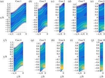
Colour contours of $\widetilde{U}(y,z)/U_{b}$ (16 contours every 0.02 units). Blue and yellow regions indicate negative and positive $\widetilde{U}(y,z)$ , respectively. The number of each case is indicated in the corresponding panels. Panels (a–e) and (f–j) correspond to cases at $Re_{h}=2500$ and 5000, respectively. The background grid has spanwise and vertical spacing of $\unicode[STIX]{x03C0}/16$ and 0.2, respectively. All the distributions are symmetric with respect to the $z/h=0$ and $z/h=-\unicode[STIX]{x1D706}/2$ planes.

In figure 7 we use the triple decomposition proposed by Finnigan (Reference Finnigan2000) to quantify the deviation of the $U$ isolines with respect to the wall-tangent direction. This decomposition was used to study turbulent flow in plant canopies by Finnigan (Reference Finnigan2000) and through urban areas by Coceal & Belcher (Reference Coceal and Belcher2004). In the present study we further decompose the mean streamwise velocity $U(y,z)$ into a wall-tangent-averaged component $\overline{U}(y)$ and its deviation from the mean $\widetilde{U}(y,z)$ such that $U(y,z)=\overline{U}(y)+\widetilde{U}(y,z)$ . The figure shows alternating patterns of regions with velocities higher (yellow) and lower (blue) than $\overline{U}$ . Near the wall, the velocity magnitude is lower in the valleys and higher in the peaks due to overlap of the boundary layer in the former and the opposite effect in the latter. Note that this effect is stronger in the cases with higher $A\unicode[STIX]{x1D714}$ values. Interestingly, regions with alternating signs are found along the vertical directions. Note that the secondary flow convects high-momentum fluid from the core of the channel to the wall along the valleys and in the opposite direction in the peaks, which could be responsible for this behaviour. Finally, the extent of these regions decreases for smaller wavelengths and wave amplitudes, and more areas with this behaviour are observed to appear from peak to valley in the cases with the largest $\unicode[STIX]{x1D706}^{+}$ values.

4 Reynolds stress distributions

Huser & Biringen (Reference Huser and Biringen1993) studied the origin of the secondary flow in square ducts by analysing the secondary Reynolds shear stresses in the horizontal wall, i.e. the shear terms involving the fluctuating spanwise component $\overline{u^{\prime }w^{\prime }}$ and $\overline{v^{\prime }w^{\prime }}$ . Marin et al. (Reference Marin, Vinuesa, Obabko and Schlatter2016) also examined these terms on the horizontal wall of the hexagonal duct. In these studies, the non-zero distributions of the secondary turbulent shear stresses were associated with inhomogeneous interaction between bursting events near the vertices of the duct. Note that the secondary Reynolds shear stresses are absent in spanwise-periodic channel flow and in vertical symmetry planes; however, they exhibit non-zero distributions near the vertices. In the sinusoidal channel, the spanwise fluctuations are only tangential to the wall at the peaks and valleys. Vidal et al. (Reference Vidal, Vinuesa, Schlatter and Nagib2017) analysed a similar scenario in ducts with rounded corners by expressing the Reynolds stress tensor in terms of the wall-normal and wall-tangent fluctuating components with respect to the closest wall. Additionally, the authors defined the local preferential direction (LPD) of the bursting events as the direction $\unicode[STIX]{x1D6FD}$ in which the turbulent in-plane shear stress $\overline{u^{\prime }u_{\unicode[STIX]{x1D6FD}}^{\prime }}$ is maximum, where $u^{\prime }$ and $u_{\unicode[STIX]{x1D6FD}}^{\prime }$ are the velocity fluctuations in the streamwise and $\unicode[STIX]{x1D6FD}$ directions, respectively. Similarly, the authors defined the direction $\unicode[STIX]{x1D6FC}$ , normal to $\unicode[STIX]{x1D6FD}$ , as the direction where the velocity fluctuations in the streamwise and $\unicode[STIX]{x1D6FC}$ -directions are uncorrelated $\overline{u^{\prime }u_{\unicode[STIX]{x1D6FC}}^{\prime }}=0$ . In so doing, they argued that streamwise momentum is preferentially transferred to the secondary flow in the local $\unicode[STIX]{x1D6FD}$ direction. In the channel with flat walls $\unicode[STIX]{x1D6FC}$ coincides with the spanwise and wall-tangent directions.

However, we will not rotate the Reynolds stress tensor, to avoid a misleading interpretation of the results in the core of the channel and to facilitate comparisons with the two-dimensional channel and the channel with riblets by Goldstein & Tuan (Reference Goldstein and Tuan1998). The distribution of the Reynolds stresses near the peaks qualitatively resembles the one found near the riblets. In the cases under study, the magnitude of $\overline{u^{\prime }v^{\prime }}$ and $\overline{u^{\prime }w^{\prime }}$ are similar and both terms can be considered as primary shear stresses as they both contribute to the wall-normal shear stress. The distributions of the Reynolds shear stresses are shown in figure 8 for the various cases under study. The maximum value of $\overline{u^{\prime }v^{\prime }}$ is always located on the peak of the channel and is flanked by the extrema of $\overline{u^{\prime }w^{\prime }}$ , located on each side of the peak. The effect of $\unicode[STIX]{x1D706}/h$ on the distribution of both quantities can be observed in the figure. As $\unicode[STIX]{x1D706}/h$ is progressively reduced, the distribution of $\overline{u^{\prime }w^{\prime }}$ shrinks and the contours of $\overline{u^{\prime }v^{\prime }}$ become increasingly horizontal. Note that the peak of $\overline{u^{\prime }v^{\prime }}$ is roughly of the same size as the non-zero distribution of $\overline{u^{\prime }w^{\prime }}$ and corresponds to the regions of intense secondary flow. In case 1, three local extrema of $\overline{u^{\prime }v^{\prime }}$ are located on the valley, side and peak of the wave, respectively, with two local $\overline{u^{\prime }w^{\prime }}$ extrema in between. These extrema progressively merge, shrink and spread in the spanwise direction as $\unicode[STIX]{x1D706}^{+}$ is reduced. The parameter $\unicode[STIX]{x1D706}/h$ has the same effect on the $\overline{u^{\prime }w^{\prime }}$ and $\overline{v^{\prime }w^{\prime }}$ distributions, i.e. they become smaller while conserving a similar magnitude and shape. Gessner (Reference Gessner1973) argued that the cross-flow is directed in the turbulent shear-stress gradient. This behaviour is also present in our results since the secondary flow is directed from the valleys to the peaks towards the extrema of $\overline{u^{\prime }v^{\prime }}$ and $\overline{u^{\prime }w^{\prime }}$ and leaves the wall in the direction of the $\overline{u^{\prime }v^{\prime }}$ gradient.

Figure 8.

Coloured contours of the primary Reynolds shear stresses $\overline{u^{\prime }v^{\prime }}^{+}$ (top half of each panel) and $\overline{u^{\prime }w^{\prime }}^{+}$ (bottom half of each panel), and (white) contours of the secondary Reynolds shear stress $\overline{v^{\prime }w^{\prime }}^{+}$ . All quantities are scaled with the averaged friction velocity $u_{\unicode[STIX]{x1D70F}}$ . Contours are separated by 0.1 units. The length and direction of the yellow lines represent the relative magnitude of the in-plane Reynolds shear stress and its direction, respectively. The case number is indicated in the corresponding panels. Panels (a–e) and (f–j) correspond to cases at $Re_{h}=2500$ and 5000, respectively. The centreline of the channel $y=A\cos (\unicode[STIX]{x1D714}z)$ is marked in grey. The background grid has spanwise and vertical spacing of $\unicode[STIX]{x03C0}/16$ and 0.2, respectively.

Figure 8 also shows a vector plot of in-plane shear stress $\overline{u^{\prime }u_{\unicode[STIX]{x1D6FD}}^{\prime }}$ indicating its relative magnitude and direction, which corresponds to the LPD of the bursting events. The LPD is normal to the wall in case 1 around $y/h\simeq 1$ , where the mean cross-flow is decelerated, indicating that bursting events have equal chances of tilting towards the peak and the valley. However, the LPD is tilted in the wall-tangent direction near the valleys and peaks such that the projection of $\overline{u^{\prime }u_{\unicode[STIX]{x1D6FD}}^{\prime }}$ in this direction points from the former to the latter. This behaviour prevents the wall-tangent fluctuations associated with the bursting events from cancelling in the mean and contributes to the production of the mean cross-flow. As $\unicode[STIX]{x1D706}/h$ is progressively reduced the LPD in the near-wall region becomes increasingly tilted with respect to the wall-normal direction, a fact that can be associated with the higher- $K$ values found in these cases. However, in cases 6 and 10, $\unicode[STIX]{x1D706}^{+}$ is too small to distort the direction of $\overline{u^{\prime }u_{\unicode[STIX]{x1D6FD}}^{\prime }}$ in a large portion of the near-wall region, where the magnitude of $\overline{u^{\prime }u_{\unicode[STIX]{x1D6FD}}^{\prime }}$ is considerable. Therefore, the cases with maximum cross-flow are those where the tilting is maximized in the entire region of high $\overline{u^{\prime }u_{\unicode[STIX]{x1D6FD}}^{\prime }}$ .

Figure 9.

Distribution of the Reynolds normal stresses. Coloured contours of the $\overline{v^{\prime 2}}^{+}$ (top half of each panel) and $\overline{w^{\prime 2}}^{+}$ (bottom half of each panel) shown every 0.2 units, and white contours of $\overline{u^{\prime 2}}^{+}$ separated by two units. All quantities are scaled with the averaged friction velocity $u_{\unicode[STIX]{x1D70F}}$ . The number of each case is indicated in the corresponding panels. Panels (a–e) and (f–j) correspond to cases at $Re_{h}=2500$ and 5000, respectively. The centreline of the channel $y=A\cos (\unicode[STIX]{x1D714}z)$ is marked in grey. The background grid has spanwise and vertical spacing of $\unicode[STIX]{x03C0}/16$ and 0.2, respectively.

The distribution of the Reynolds normal stresses is shown in figure 9. The bursting events are part of the near-wall cycle of turbulence, responsible for the inner peak of the streamwise velocity fluctuations $\overline{u^{\prime 2}}$ ; see Jiménez & Moin (Reference Jiménez and Moin1991) and Pope (Reference Pope2000). The maximum value of this quantity is always located around the peaks, indicating that bursting events are stronger and more frequent in this region. Therefore, the instantaneous streamwise vortices associated with the bursting events near the peaks are not cancelled in the mean by the weaker adjacent vortices located farther towards the valleys. This behaviour is illustrated in the right-hand panels of figure 1 and is not present in the channel with flat walls, where the distribution of $\overline{u^{\prime 2}}$ is homogeneous in the spanwise direction. Again in case 1, $\overline{u^{\prime 2}}$ is homogeneous in the wall-tangent direction around $y/h\simeq 1$ and becomes increasingly inhomogeneous as $\unicode[STIX]{x1D706}/h$ is reduced in the other cases. Similarly, in cases 6 and 10, with the smallest $\unicode[STIX]{x1D706}^{+}$ , the isolines of $\overline{u^{\prime 2}}$ away from the wall are parallel to the spanwise direction, a fact that indicates that the largest bursting events are no longer contributing to the production of mean cross-flow. A similar behaviour is observed in the distributions of the vertical $\overline{v^{\prime 2}}$ and spanwise $\overline{w^{\prime 2}}$ fluctuations. Note that the cross-partial derivatives of $\overline{v^{\prime 2}}-\overline{w^{\prime 2}}$ generate $\unicode[STIX]{x1D6FA}_{x}$ in (1.1). Figure 9 shows that if $\unicode[STIX]{x1D706}^{+}$ is reduced beyond a certain limit, roughly around 150 viscous units, these distributions become increasingly homogeneous in the spanwise direction, as can be appreciated when going from cases 2 to 3, 5 to 6 and 9 to 10.

Figure 10.

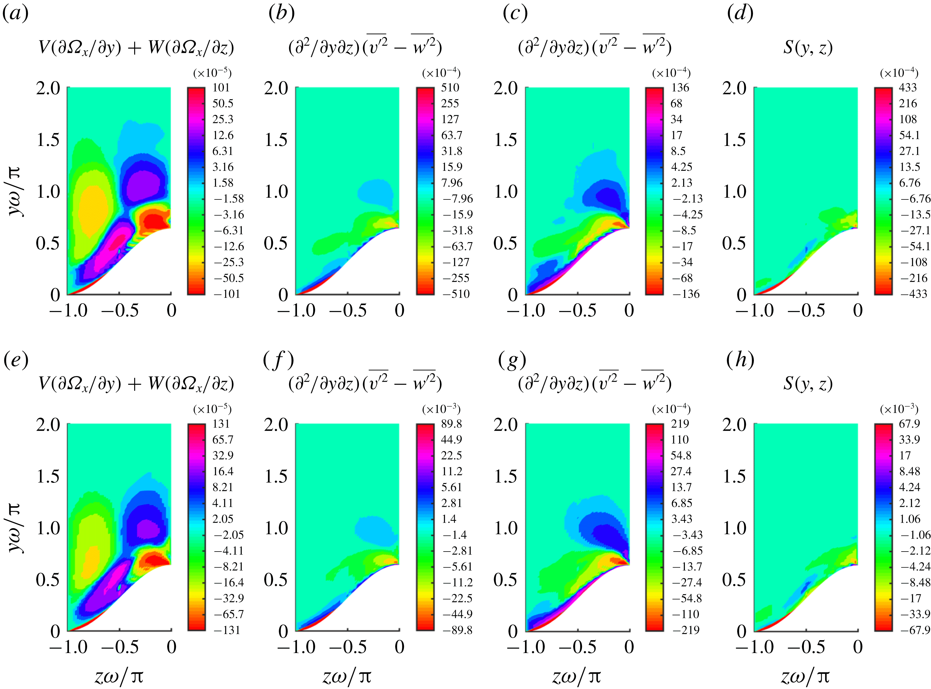
Coloured contours of the terms in (1.1) scaled in viscous units for cases (top) 3 and (bottom) 6 and using a binary logarithmic colour scale.

The secondary Reynolds shear stress $\overline{v^{\prime }w^{\prime }}$ and the anisotropy of the cross-stream deviatoric Reynolds stress $\overline{v^{\prime 2}}-\overline{w^{\prime 2}}$ are related to $\unicode[STIX]{x1D6FA}_{x}$ in the first and second terms on the right-hand side of (1.1), which are shown in figure 10 for cases 3 and 6. These terms can be grouped into a single source term $S(y,z)$ , which is defined in (4.1) and also shown in the figure. The term $S$ forms pairs of sources ( $S>0$ ) and sinks ( $S<0$ ) of $\unicode[STIX]{x1D6FA}_{x}$ in the near-wall region that alternate in the wall-tangent direction. Figure 10 also shows the transport of $\unicode[STIX]{x1D6FA}_{x}$ by the secondary flow or left-hand side of the equation. Near the wall, the secondary flow convects $\unicode[STIX]{x1D6FA}_{x}$ in a direction which is roughly normal to its gradient. Therefore, the magnitude of the left-hand side is much smaller than the magnitude of $S$ , and most of $\unicode[STIX]{x1D6FA}_{x}$ in this region is diffused from the sources to sinks along the wall leading to the stronger inner peak of $\unicode[STIX]{x1D6FA}_{x}$ . Scaling all the variables in (1.1) in viscous units except for $\unicode[STIX]{x1D6FA}_{x}^{\ast }=\unicode[STIX]{x1D6FA}_{x}\unicode[STIX]{x1D706}/u_{\unicode[STIX]{x1D70F}}$ leads to (4.2), where the parameter $1/\unicode[STIX]{x1D706}^{+}$ acts as a vorticity-diffusivity coefficient. Note that $\unicode[STIX]{x1D6FA}_{x}$ depends on $\unicode[STIX]{x1D706}^{+}$ , as shown in figure 6 and table 3. As $\unicode[STIX]{x1D706}^{+}$ increases the diffusivity parameter decreases and $\unicode[STIX]{x1D6FA}_{x}$ is confined to a region closer to the wall.

(4.1) $$\begin{eqnarray}\displaystyle & \displaystyle S(y,z)=\frac{\unicode[STIX]{x2202}^{2}}{\unicode[STIX]{x2202}y\unicode[STIX]{x2202}z}(\overline{v^{\prime 2}}-\overline{w^{\prime 2}})-\left(\frac{\unicode[STIX]{x2202}^{2}}{\unicode[STIX]{x2202}y^{2}}-\frac{\unicode[STIX]{x2202}^{2}}{\unicode[STIX]{x2202}z^{2}}\right)\overline{v^{\prime }w^{\prime }}, & \displaystyle\end{eqnarray}$$

(4.2) $$\begin{eqnarray}\displaystyle & \displaystyle V^{+}\frac{\unicode[STIX]{x2202}\unicode[STIX]{x1D6FA}_{x}^{\ast }}{\unicode[STIX]{x2202}y^{+}}+W^{+}\frac{\unicode[STIX]{x2202}\unicode[STIX]{x1D6FA}_{x}^{\ast }}{\unicode[STIX]{x2202}z^{+}}=S^{+}+\frac{1}{\unicode[STIX]{x1D706}^{+}}\unicode[STIX]{x1D6FB}^{2}\unicode[STIX]{x1D6FA}_{x}^{\ast }. & \displaystyle\end{eqnarray}$$

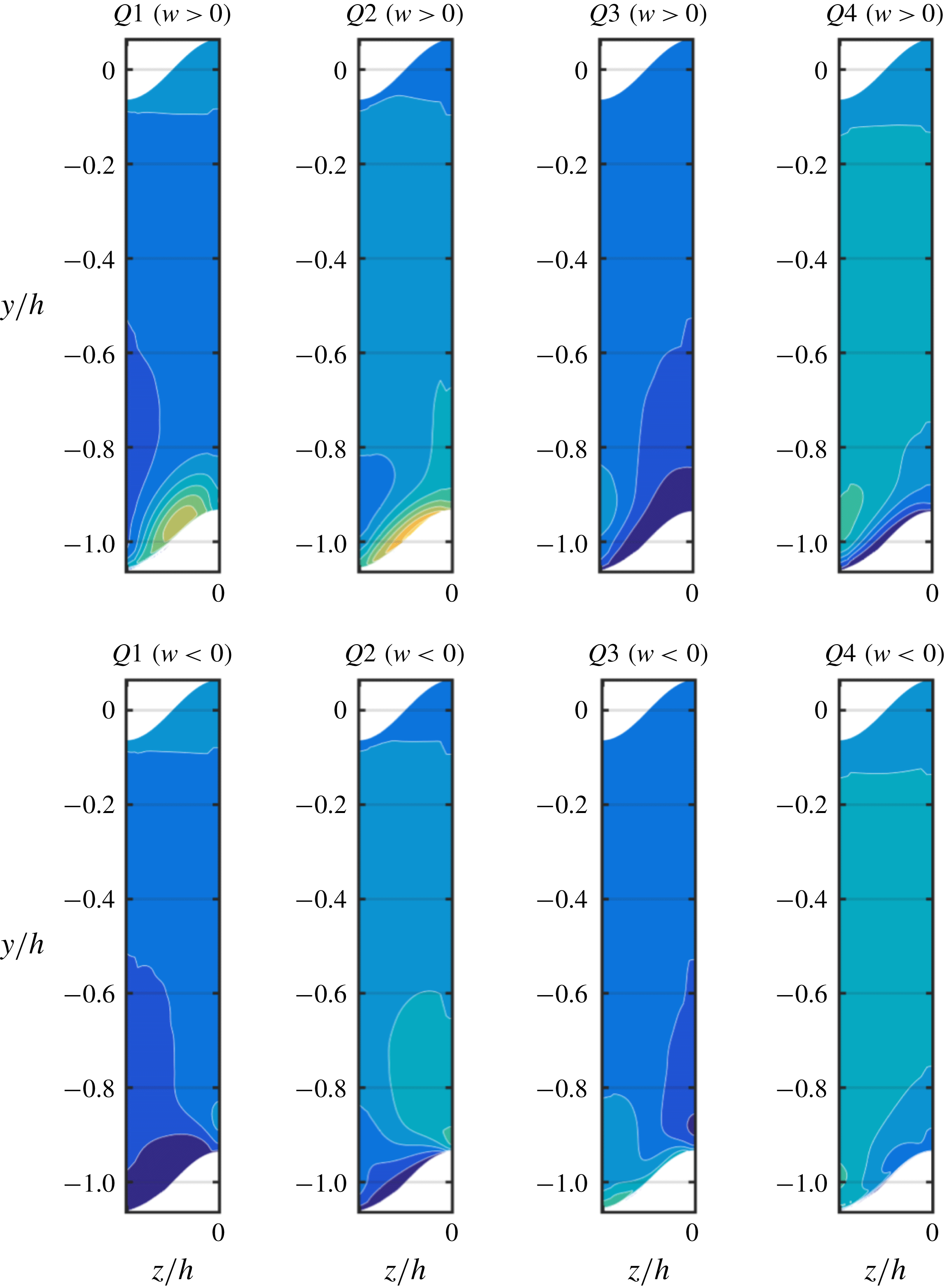
5 Probability density function of the events related to the bursting process

Table 4.

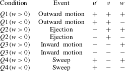
Flow conditions used for conditional averaging.

By analysing the mechanisms responsible for the distributions of the turbulent stresses, shown in figures 8 and 9, we can gain more insight into the origin of the secondary flow. To this end, we calculated the probability density function (pdf) associated with the eight conditions shown in table 4. The pdf is normalized such that that the sum of all the pdf distributions is equal to one. In a turbulent channel with straight walls, bursting events can be classified into four categories ( $Q1$ – $Q4$ in table 4) depending on the sign of the streamwise and vertical fluctuating components, see Lu & Willmarth (Reference Lu and Willmarth1973) and Kim (Reference Kim1985). Note that in this study we extend this classification to eight cases by analysing the sign of the spanwise component. Bursting events were recently analysed by Farano et al. (Reference Farano, Cherubini, Robinet and De Palma2017) in turbulent channel flow and by Jelly, Jung & Zaki (Reference Jelly, Jung and Zaki2014) in turbulent channel flow with streamwise-aligned superhydrophobic surface texture. Note that in the absence of secondary flow the instantaneous and fluctuating cross-stream velocity components are equal, i.e. $v=v^{\prime }$ and $w=w^{\prime }$ . The most frequent type of events are sweeps ( $u^{\prime }>0$ , $v<0$ ) and ejections ( $u^{\prime }<0$ , $v>0$ ). Sweeps or $Q4$ events convect energetic fluid ( $u^{\prime }>0$ ) from the core of the channel into the near-wall region ( $v<0$ ). As they approach the wall, sweeping events turn in the wall-tangent direction. In the channel with straight walls, sweeping events are as likely to turn in the positive and negative spanwise directions. On the other hand, ejections or $Q2$ events convect low-momentum fluid ( $u^{\prime }<0$ ) from the near-wall region into the core of the channel ( $v>0$ ) and are also as likely to tilt in the positive and negative spanwise directions of the straight wall channel. However, in the channel with sinusoidal walls the bursting events preferentially tilt towards the peaks. In order to quantify this preferential behaviour we have further characterized the events with respect to the sign of their instantaneous spanwise velocity such that $Q2\;(w>0)$ are ejections with positive spanwise instantaneous velocity. The pdf distributions are calculated with samples of the instantaneous velocity fields obtained every 2 convective time units for the averaging periods shown in table 1. The results are averaged in the streamwise direction and the periodicities of the wall geometry are used to increase the number of samples by a factor of $2\unicode[STIX]{x1D714}$ . 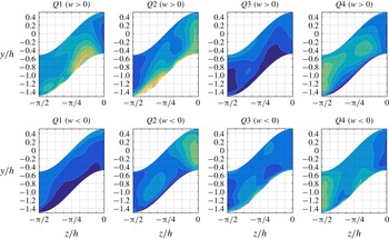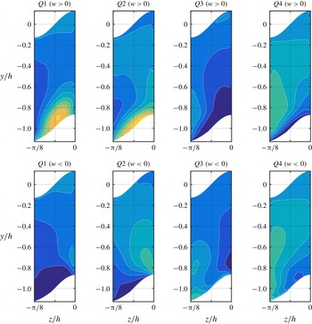The corresponding pdf distributions are shown in figures 11, 12 and 13 for cases 1, 3 and 6, respectively.

Figure 11.

Contours every 0.04 units showing the pdf of events related to the bursting process corresponding to flow case 1. The corresponding conditions are shown in each panel as indicated in table 4.

In all the cases under study, spanwise inhomogeneous distributions and tilting of the bursting events are observed. We denote a certain type of bursting event $Q$ as inhomogeneously distributed if it is preferentially located at a specific spanwise position, thus $\unicode[STIX]{x2202}(pdf[Q])/\unicode[STIX]{x2202}z\neq 0$ . Similarly, we denote a bursting event $Q$ as exhibiting inhomogeneous tilting if $pdf[Q(w>0)]\neq pdf[Q(w<0)]$ , i.e. the bursting event preferentially develops in either spanwise directions. Our results show that bursting events located between the valleys and the peaks preferentially develop from the former to the later such that $pdf[Q(w>0)]>pdf[Q(w<0)]$ , generating the region of strong $\overline{u^{\prime }w^{\prime }}>0$ which is observed in the bottom half of each panel in figure 8. Therefore, both regions shrink equally as $\unicode[STIX]{x1D706}/h$ is reduced. Additionally, sweeping events and ejections are preferentially located in the valleys and peaks, respectively. Ejections are the main contributors to the region of strong $\overline{u^{\prime }v^{\prime }}$ near the peaks, a result that is shown on the top half of each panel in figure 8. These events are equally likely to turn in the positive and negative spanwise directions, since they occur at symmetry planes. However, their associated streamwise vortices contribute not only to the wall-normal but also to the wall-tangent cross-flow. The ejections that tilt in the negative spanwise direction generate the region of $\unicode[STIX]{x1D6FA}_{x}<0$ shown in figure 4, which is associated with the change of direction of the cross-flow near the peaks. Note that the $\unicode[STIX]{x1D6FA}_{x}$ distribution is antisymmetric with respect to the centreplane of the peaks and valleys; thus the ejections that tilt towards the positive spanwise direction will generate $\unicode[STIX]{x1D6FA}_{x}>0$ on the other side, and will also contribute to the mean cross-flow. On symmetry planes, sweeps also turn in either the positive or negative spanwise directions, producing the outer region of $\unicode[STIX]{x1D6FA}_{x}<0$ , on the right, and $\unicode[STIX]{x1D6FA}_{x}>0$ , on the left of the centreplane of the valley, respectively. This mechanism causes the secondary flow to turn in the wall-tangent direction towards the peaks.

Figure 12.

Contours every 0.04 showing the pdf of events related to the bursting process corresponding to the flow case 3. The corresponding conditions are shown in each panel as indicated in table 4.

Note that the average number of simultaneous bursting events between the valleys and peaks is determined by the parameter $\unicode[STIX]{x1D706}^{+}/2$ . In case 1, $\unicode[STIX]{x1D706}^{+}/2$ is large enough to fit a sequence of sweeps and ejections from the valley to the peak, as shown in figure 11. The sequence starts with the sweeping event located in the valley, which is followed by an ejection at a rough distance of 60 viscous units in the wall-tangent direction. This sweep/ejection pattern was identified by Vidal et al. (Reference Vidal, Vinuesa, Schlatter and Nagib2018) in turbulent ducts with rounded corners starting with a sweeping event at the transition from curved to straight walls and followed by an ejection at the beginning of the straight wall. The ejection is the main contributor to the extrema of $\overline{u^{\prime }w^{\prime }}$ located near the valley. Another sweeping event is preferentially located between $y/h\simeq 1$ and the peak. Note that $Q1\;(w>0)$ can also be considered as a sweeping event since $w>0$ on the side of the wave is directed towards the wall. Therefore, the sweeps of type $Q1\;(w>0)$ and $Q3\;(w>0)$ generate the maximum value of $\overline{u^{\prime }w^{\prime }}$ , which is located near the peak. The resulting sequence from valley to peak in case 1 is sweep/ejection/sweep/ejection.

Figure 13.

Contours every 0.04 units showing the pdf of events related to the bursting process corresponding to the flow case 6. The corresponding conditions are shown in each panel as indicated in table 4.

However, as $\unicode[STIX]{x1D706}^{+}/2$ is reduced, the inner-scaled length of the wall is not large enough to fit four simultaneous bursting events. Instead, the instantaneous cross-flow is directed into the valleys by sweeping events, turns towards the peaks generating $\overline{u^{\prime }w}$ along the side, and is driven towards the core by ejections producing $\overline{u^{\prime }v}$ on the peak. Note that for converged turbulence statistics $\overline{u^{\prime }w}=\overline{u^{\prime }w^{\prime }}$ and $\overline{u^{\prime }v}=\overline{u^{\prime }v^{\prime }}$ . This integrated behaviour is appreciated in the merging of the $\unicode[STIX]{x1D6FA}_{x}$ extrema associated with the valleys and peaks and the collapse of the $\unicode[STIX]{x1D6F9}$ and $\unicode[STIX]{x1D6FA}_{x}$ distributions. Uhlmann et al. (Reference Uhlmann, Pinelli, Kawahara and Sekimoto2007) showed that if the inner-scaled width of the square duct is not large enough to fit more than three simultaneous velocity streaks, the secondary-flow pattern is a direct consequence of the coherent buffer-layer structures. Therefore, our results show that marginally turbulent flow effects can be induced at higher Reynolds number by means of a sinusoidal wall with marginal $\unicode[STIX]{x1D706}^{+}$ values. Note that if $\unicode[STIX]{x1D706}/h\rightarrow 0$ and $\unicode[STIX]{x1D706}^{+}\simeq 150$ the cross-flow only depends on the near-wall structures, thus similar results are expected at larger Reynolds numbers. Marginally turbulent flow effects could be responsible for the enhanced cross-flow in case 3, which is the case with the strongest secondary flow. The works by Marin et al. (Reference Marin, Vinuesa, Obabko and Schlatter2016) and Vidal et al. (Reference Vidal, Vinuesa, Schlatter and Nagib2017) show a similar effect in turbulent hexagonal ducts and square ducts with rounded corners, respectively. In this case, the regions of inhomogeneous distribution and tilting coincide with the region in which the turbulent stresses are stronger. Therefore, the mechanisms responsible for the turbulent stresses also contribute to the mean cross-flow. However, if $\unicode[STIX]{x1D706}^{+}/2$ is not large enough to fit the largest bursting events, the regions of maximum turbulent stresses and inhomogeneous behaviour do not completely overlap. This behaviour can be clearly appreciated in case 6 by comparing its pdf distributions, shown in figure 13, to its Reynolds stresses, shown in figures 8 and 9. In this case, the bursting events exhibit an approximately homogeneous behaviour above $y/h>-0.6$ , where the Reynolds stresses are very strong. Furthermore, the turbulent stresses become nearly homogeneous in the spanwise direction at $y/h>0.6$ , and do not contribute to the secondary flow. Therefore, the value of $\unicode[STIX]{x1D706}^{+}$ must be larger than the mean wavelength of the bursting cycle to promote wall-tangent preferential behaviour among the largest and most energetic bursting events, in order to maximize the kinetic energy of the mean cross-flow $K$ and the total cross-flow rate $Q_{yz}$ .

6 Cross-flow rate model

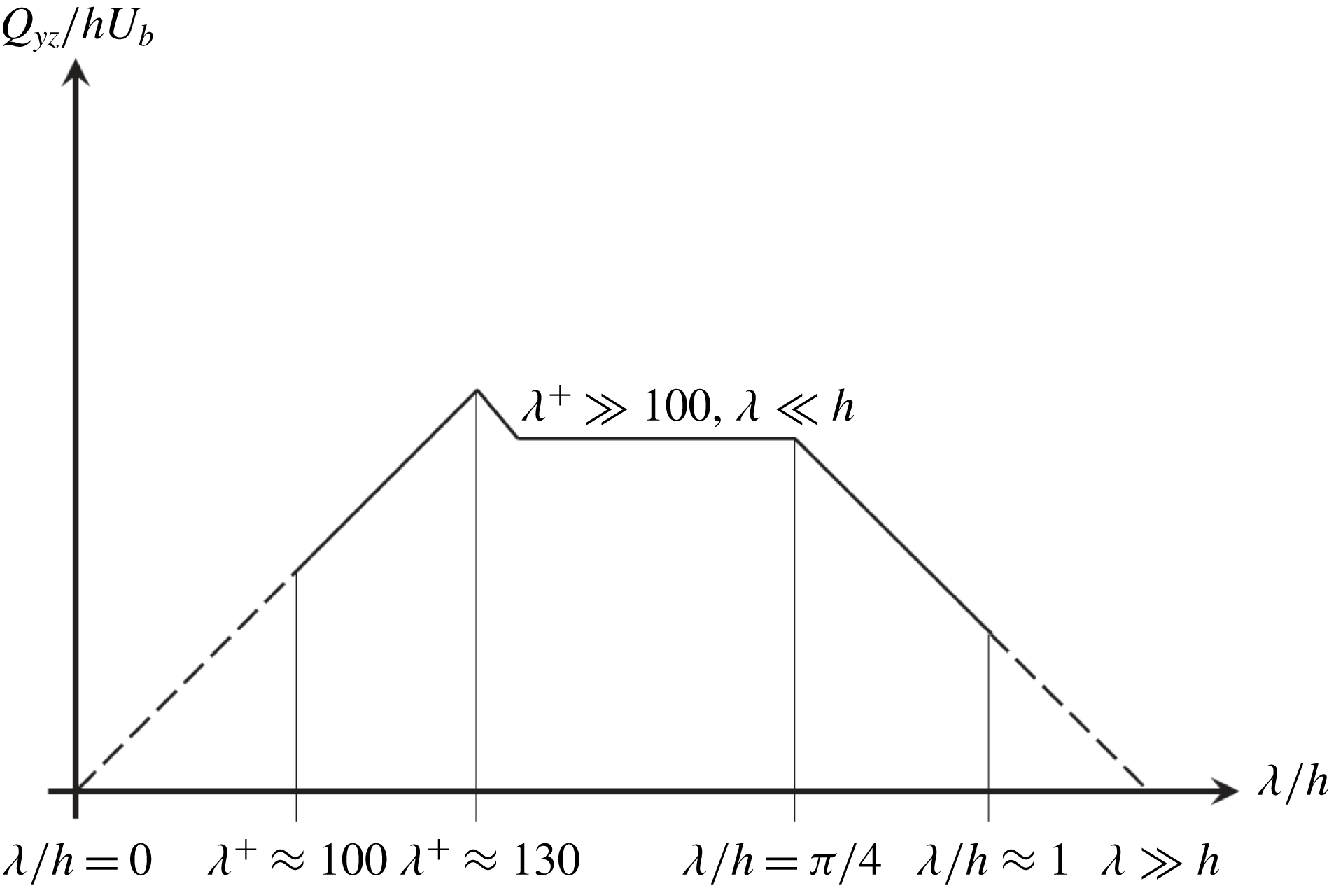
A theoretical model to characterize the total cross-flow rate $Q_{yz}/(hU_{b})$ , based on the results discussed in this study, is shown in figure 14. The model indicates that the mean cross-flow must be absent if $\unicode[STIX]{x1D706}/h=0$ or $\unicode[STIX]{x1D706}\gg h$ . As $\unicode[STIX]{x1D706}\rightarrow 0$ the geometry of the wall converges to spanwise-homogeneous roughness, as discussed in the previous sections and observed in riblets with decreasing separation (Goldstein & Tuan Reference Goldstein and Tuan1998). Similarly, if $\unicode[STIX]{x1D706}\gg h$ the local geometry of the wall can be considered as flat with respect to $h$ . Therefore, the secondary flow develops if $\unicode[STIX]{x1D706}$ is not much larger than $h$ and is larger than the smallest scales in the flow. Consequently, a value of $\unicode[STIX]{x1D706}$ exists such that $Q_{yz}$ is maximum.

Figure 14.

Qualitative behaviour of the total cross-flow rate $Q_{yz}/(hU_{b})$ as a function of the wavelength $\unicode[STIX]{x1D706}$ . The solid lines show the trends from the cases summarized in table 3, and the dashed lines are extrapolations based on theoretical arguments.

The studies by Uhlmann et al. (Reference Uhlmann, Pinelli, Kawahara and Sekimoto2007), Pinelli et al. (Reference Pinelli, Uhlmann, Sekimoto and Kawahara2010), Vinuesa et al. (Reference Vinuesa, Noorani, Lozano-Durán, El Khoury, Schlatter, Fischer and Nagib2014) and Zhang et al. (Reference Zhang, Trias, Gorobets, Tan and Oliva2015) in square ducts, by Vidal et al. (Reference Vidal, Vinuesa, Schlatter and Nagib2017) in square ducts with rounded corners and by Marin et al. (Reference Marin, Vinuesa, Obabko and Schlatter2016) in hexagonal ducts show that $\unicode[STIX]{x1D6F9}_{max}/(hU_{b})$ is not sensitive to changes in the Reynolds number if $Re_{\unicode[STIX]{x1D70F},c}$ is large enough to prevent marginally turbulent flow effects. Note that $\unicode[STIX]{x1D6F9}_{max}$ determines $Q_{yz}$ in cases with the same geometry. This behaviour is observed by comparing cases 2 and 4, which have the same wall geometry and $\unicode[STIX]{x1D6F9}_{max}$ values and where $Re_{h}$ is increased by a factor of two. Therefore, if the separation between the smallest scales and $\unicode[STIX]{x1D706}$ is large enough $Q_{yz}$ must only depend on $\unicode[STIX]{x1D706}/h$ . Our results show that $Q_{yz}/(hU_{b})$ is inversely proportional to $\unicode[STIX]{x1D706}/h$ in a range $\unicode[STIX]{x03C0}/4<\unicode[STIX]{x1D706}/h<\unicode[STIX]{x03C0}$ (where this upper limit is taken as $\unicode[STIX]{x1D706}\sim h$ in figure 14). Note that if $Re_{h}$ is large enough to disregard marginally turbulent flow effects, the slope of $Q_{yz}$ with $\unicode[STIX]{x1D706}/h$ is similar at any $Re_{h}$ . In fact, our results show that the slope in the $Q_{yz}/(hU_{b})$ versus $\unicode[STIX]{x1D706}/h$ model from figure 14 is equal to $-1$ between $\unicode[STIX]{x1D706}\approx \unicode[STIX]{x03C0}/4$ and $\unicode[STIX]{x1D706}^{+}\approx \unicode[STIX]{x03C0}$ . In § 3 we showed that as the secondary vortices become smaller their total cross-flow rate and angular momentum are conserved, thus $Q_{yz}$ increases due to the addition of more vortices in the spanwise direction. This acceleration of the vortices must be limited by the outer-scaled wavelength $\unicode[STIX]{x1D706}/h$ , since the magnitude of the mean cross-flow cannot exceed that of the instantaneous cross-flow $(K/k<1)$ .

The results from the authors cited above show that marginally turbulent flow effects lead to higher $\unicode[STIX]{x1D6F9}_{max}$ and $Q_{yz}$ . This behaviour is appreciated by comparing cases 3 and 5 or cases 8 and 9, which also have the same wall geometry but where $Q_{yz}/(hU_{b})$ is increased by a factor of 1.2 in the cases with lower $Re_{h}$ , where marginally turbulent flow effects are dominant. In these cases, $Q_{yz}/(hU_{b})$ is maximum and $\unicode[STIX]{x1D706}^{+}\simeq 130$ , which is barely large enough to fit two near-wall counter-rotating vortices. As discussed in §§ 4 and 5, $\unicode[STIX]{x1D706}^{+}\simeq 130$ maximizes inhomogeneous interaction of the bursting events throughout the wall and prevents these vortices from cancelling on the mean.

Since the increasing slope of $Q_{yz}$ with $\unicode[STIX]{x1D706}/h$ is not sensitive to $Re_{h}$ and the maximum $Q_{yz}/(hU_{b})$ value corresponds to $\unicode[STIX]{x1D706}^{+}\simeq 130$ , but is limited by $\unicode[STIX]{x1D706}/h$ , it is reasonable to assume that if $\unicode[STIX]{x1D706}^{+}\gg 100$ and $\unicode[STIX]{x1D706}\ll h$ the value of $\unicode[STIX]{x1D6F9}_{max}/(\unicode[STIX]{x1D706}U_{b})$ and $Q_{yz}/(hU_{b})$ is constant. Note that in the present cases the separation of scales is not large enough to completely appreciate this region and more cases are required at higher Reynolds numbers and with smaller $\unicode[STIX]{x1D706}/h$ values to fully characterize this behaviour. However, a similar behaviour is observed by comparing cases 5 and 6, where $\unicode[STIX]{x1D706}/h=\unicode[STIX]{x03C0}/4$ and $\unicode[STIX]{x03C0}/8$ , respectively. In this range, the reduced cross-flow rate $\unicode[STIX]{x1D6F9}_{max}/(hU_{b})$ associated with each secondary vortex is compensated by the presence of more vortices such that $\unicode[STIX]{x1D6F9}_{max}/(\unicode[STIX]{x1D706}U_{b})$ and $Q_{yz}/(hU_{b})$ are constant.