1 Introduction
The level of convective overshooting is important in modelling stellar evolution, where it determines the amount of material entrained into turbulent regions (Böhm-Vitense Reference Böhm-Vitense1958; Cloutman Reference Cloutman1987). Once within a convective layer, fresh material may be transported into the core of a star where nuclear fusion can take place, extending the burning lifetime of the star, or outwards into the stellar envelope, enriching this material with heavier elements. This may have a direct effect on the structure of such stars, the stellar wind mass loss from them and on the amount of material processed by fusion reactions which is ejected into the interstellar medium at the end of the star’s life. Mixing is also important for pollutant transport in the terrestrial troposphere, where turbulence in regions with close to neutral stability can be strongly confined by strong stratification in elevated temperature inversions (Reible Reference Reible1998, p. 300).
A series of experiments have been undertaken to study this process by Davies Wykes, Lawrie and Dalziel at the University of Cambridge (Lawrie & Dalziel Reference Lawrie and Dalziel2011; Davies Wykes & Dalziel Reference Davies Wykes and Dalziel2014). These experiments were done in a water tank, which has two compartments separated by a horizontal barrier. In a typical Rayleigh–Taylor experiment, the upper compartment is filled with a solution with higher density than the lower, so that when the barrier is removed, buoyancy-driven mixing ensues. In the experiments which are of interest in the present work, a stable density stratification was imposed above and below the barrier, so that the growth of the mixing layer was limited by the level to which it could entrain material from the exterior density stratification, rather than by the vertical extent of the tank as in more typical uniform-density Rayleigh–Taylor experiments (Dalziel, Linden & Youngs Reference Dalziel, Linden and Youngs1999).
In this paper, we study the late-time density structure of mixing layers confined by density stratification, rather than by the rigid boundaries of the experiment. We develop a model for this structure based on the maximization of a configurational entropy functional. To provide comparison data, we have performed calculations using the Eulerian hydrodynamics code TURMOIL (Youngs Reference Youngs1991). This code implements a low dissipation, staggered mesh scheme, which we use to perform high-resolution monotone implicit large eddy simulations (hereafter MILES). We refer the reader to numerous previous papers for detailed discussion of the use of the MILES methodology in modelling high Reynolds number turbulent flows (Margolin & Rider Reference Margolin and Rider2002; Grinstein, Margolin & Rider Reference Grinstein, Margolin and Rider2007; Youngs Reference Youngs2009).
Our results complement the numerical studies already performed by Davies Wykes, Lawrie & Dalziel. They have been performed with an independent code, at somewhat higher resolution (800 zones vertically compared to 512) and over a domain with twice the lateral dimension (equal to the height of the domain in both directions), which should improve the statistical convergence of our results. (A run with double the mesh resolution for the case with linear stratification confirms that the numerical results presented here do not depend strongly on the mesh resolution we have chosen.)
The general agreement of the results of these calculations with experiment is good. We have not replicated all the calculations performed previously, as it is not the intent of the present paper to duplicate this previous work. Instead, to broaden the comparison with our physical model, we consider forms of the initial density profile and perturbations which have not been studied experimentally to date, to investigate issues such as whether the symmetry of the initial conditions is significant in determining the form of the late-stage equilibrium profile.
We then develop a simple model for the equilibrium structure of the mixing layers at late times, based on applying ideas from statistical physics, and compare this to our numerical results.
2 Problem specification and numerical scheme
2.1 Stratification and initial conditions
We have performed calculations of mixing layer growth with a number of forms for the stratification and initial conditions. While the experiments were performed with nearly incompressible aqueous solutions with Atwood numbers between
 $4\times 10^{-3}$
and
 $7\times 10^{-2}$
(Davies Wykes & Dalziel Reference Davies Wykes and Dalziel2014), the present calculations are at a moderate Atwood number of
 $A_{0}=0.091$
, where
 $A_{0}=(\unicode[STIX]{x1D70C}_{2}-\unicode[STIX]{x1D70C}_{1})/(\unicode[STIX]{x1D70C}_{2}+\unicode[STIX]{x1D70C}_{1})$
(i.e. a density ratio of 1.2:1), and assume that the materials have a compressible perfect gas equation of state with
 $\unicode[STIX]{x1D6FE}=5/3$
. The maximal Mach number of the flows in our calculations is
 ${\sim}0.1$
, so the calculations are close to incompressible; however, it should be noted that the calculations are being performed with the aim of exploring the physics of Rayleigh–Taylor mixing between stratified mixing layers, rather than with the intention of achieving a detailed match to the experimental results. Given the explicit hydrodynamics scheme used by TURMOIL, it is far more numerically efficient to perform this study using flows at a Mach numbers
 ${\sim}0.1$
where the incompressible flow assumption is still expected to be accurate.
The initial stratified structure is assumed to obey the equation of hydrostatic equilibrium
 $$\begin{eqnarray}\frac{\text{d}p}{\text{d}h}=-\unicode[STIX]{x1D70C}g,\end{eqnarray}$$
where
 $p$
is the pressure,
 $h$
is the vertical coordinate (this will also be referred to
 $x$
in the context of the three-dimensional numerical calculations),
 $\unicode[STIX]{x1D70C}$
is the density and
 $g$
is the gravitational acceleration. This means that for an imposed density stratification, the pressure field is also determined. The equation of state of the material is important in determining the stability of the stratification. If the material is assumed to have a polytropic equation of state with index
 $\unicode[STIX]{x1D6FE}$
(as for example
 $5/3$
in the present calculations), then the density stratification is convectively stable if it satisfies the Schwarzschild criterion (Schwarzschild Reference Schwarzschild1906, Reference Schwarzschild1958; Kaniel & Kovetz Reference Kaniel and Kovetz1967)
 $$\begin{eqnarray}\frac{\text{d}(\ln \unicode[STIX]{x1D70C})}{\text{d}(\ln p)}=-\frac{p}{\unicode[STIX]{x1D70C}^{2}g}\frac{\text{d}\unicode[STIX]{x1D70C}}{\text{d}h}=-(\unicode[STIX]{x1D6FE}-1)c_{v}\frac{T}{\unicode[STIX]{x1D70C}g}\frac{\text{d}\unicode[STIX]{x1D70C}}{\text{d}h}>\frac{1}{\unicode[STIX]{x1D6FE}},\end{eqnarray}$$
where
 $\unicode[STIX]{x1D6FE}$
is the local value of the effective adiabatic coefficient,
 $c_{v}$
the specific heat and
 $T$
the temperature, i.e.
 $$\begin{eqnarray}\frac{\text{d}p/\text{d}h}{\text{d}\unicode[STIX]{x1D70C}/\text{d}h}<c_{s}^{2},\end{eqnarray}$$
where
 $c_{s}$
is the adiabatic sound speed.
The interpretation of this is that if a parcel of gas is raised adiabatically through the pressure stratification, for stability its density must decrease less than the density decrease in the surrounding static material (assuming that thermal transport between parcels of material is negligible) – otherwise, it will become buoyant and continue to rise. Note that, when specified in terms of the density gradient, this criterion is equivalent to the Ledoux criterion for convective instability (Ledoux Reference Ledoux1947), which takes into account variations in the molecular mass of the material: as typically applied, these criteria are based on the temperature stratification rather than the density stratification, and the canonical form of the Schwarzschild criterion results if the dependence of the equation of state on the mean molecular mass is not taken into account.
This stability criterion given by (2.3) is similar to that for Rayleigh–Taylor stability (Rayleigh Reference Rayleigh1882; Taylor Reference Taylor1950)
 $$\begin{eqnarray}\frac{\text{d}\unicode[STIX]{x1D70C}}{\text{d}h}\frac{\text{d}p}{\text{d}h}>0,\end{eqnarray}$$
i.e.
 $$\begin{eqnarray}\frac{\text{d}\unicode[STIX]{x1D70C}}{\text{d}p}>0,\end{eqnarray}$$
but is more restrictive on the zone of stability (i.e. it is possible for Rayleigh–Taylor stable flows to be convectively unstable if the fluid is sufficiently compressible). The corresponding correction to the buoyancy source term for compressible turbulence models has been applied on occasion (Andronov et al. Reference Andronov, Bakhrakh, Mokhov, Nikiforov and Pevnitskii1979; Cloutman Reference Cloutman1987), but is not in widespread use.
In this paper, we will assume that the initial stratification to be isothermal. For an arbitrary density profile, the molecular mass must then vary with position. The easiest way of achieving this within TURMOIL is to specify that all the materials are initially mixtures of materials with different molecular masses. This may be achieved by using two materials, but (as in the experiment) an additional advected passive scalar field is then required to track the interfacial mixing. The initial interface is established by a discontinuous change in mean molecular mass. On either side of the interface, the materials will be convectively stable for this isothermal stratification so long as there is not an extreme gradient in molecular mass
 $\unicode[STIX]{x1D707}_{m}$
,
 $$\begin{eqnarray}\frac{\text{d}\ln \unicode[STIX]{x1D707}_{m}}{\text{d}\ln p}>\frac{1}{\unicode[STIX]{x1D6FE}}-1.\end{eqnarray}$$
We simulate a box of size 2 units in each dimension. In the direction of gravity, we use reflective boundaries at
 $x=\pm 1$
(so that there is zero fluid velocity through the boundaries, but free slip along them), while in the
 $y$
and
 $z$
directions we assume periodic boundary conditions. We take the gravitational acceleration in the test problem to be
 $g_{x}=g=1$
, and the interface pressure to be
 $p=300$
, which means that the calculations should be close to incompressible, since
 $gH/c^{2}\simeq 1/250$
, with
 $H=2$
the total height of the domain.
We consider four distinct profiles, which are most clearly seen as the initial time profiles plotted in figure 5. These were:
-
(a) a linear density profile on above and below the interface;
-
(b) quadratic profiles above and below the interface, tending from uniform at the external boundary to a steep dependence close to the interface;
-
(c) as (b), except with the slower density variation in the lower part of the domain close to the interface;
-
(d) as (a), except with the density variation close to the interface clipped to
 $\pm 0.02$
units of the mean density.

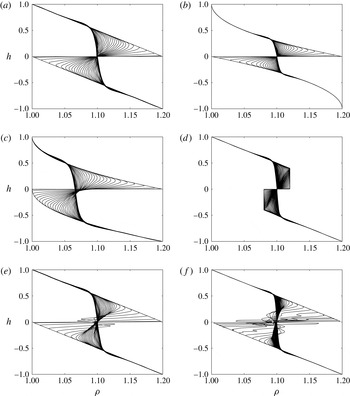
These cases can be understood more clearly by referring to figure 5. We also consider additional linear density profile calculations with an additional regular
 $\unicode[STIX]{x1D706}=0.2$
perturbation across one dimension of the mesh, with different amplitudes, (e) and (f); in case (f), the perturbation amplitude saturated at a certain level (a case without this saturation behaviour was also run, but the results with the saturated profile seemed more interesting, as we will discuss below). Cases (a) and (b) relate to experimental conditions considered by Davies Wykes & Dalziel (Reference Davies Wykes and Dalziel2014), the comparison with which validates our numerical modelling. The other profiles have been chosen to allow us to study the robustness of our conclusions on the energetics and flow structure for a wider class of distributions than were considered in the experimental work, i.e. to address questions on whether the final structure depends on the symmetry, initial Atwood number or level of surface perturbation in the initial conditions.
The density stratification is defined to run from
 $\unicode[STIX]{x1D70C}=1$
to
 $\unicode[STIX]{x1D70C}=1.2$
across each layer for all cases apart from the truncated profile. For example, for the linearly stratified case,
 $$\begin{eqnarray}\unicode[STIX]{x1D70C}=\left\{\begin{array}{@{}ll@{}}1.2-0.2h, & h\geqslant 0,\\ 1.0-0.2h, & h<0,\end{array}\right.\end{eqnarray}$$
and
 $$\begin{eqnarray}p=\left\{\begin{array}{@{}ll@{}}300-1.2h+0.1h^{2}, & h\geqslant 0,\\ 300-1.0h+0.1h^{2}, & h<0.\end{array}\right.\end{eqnarray}$$
Together with the perfect gas equation of state
 $$\begin{eqnarray}p=nk_{B}T=\frac{\unicode[STIX]{x1D70C}}{\unicode[STIX]{x1D707}_{m}}k_{B}T,\end{eqnarray}$$
where
 $n$
is the particle density and
 $k_{B}$
the Boltzmann constant, and the assumption that the initial stratification is isothermal, this specifies the profile of molecular mass
 $\unicode[STIX]{x1D707}_{m}$
, and hence the mass fraction
 $m_{1}$
 $$\begin{eqnarray}m_{1}=\frac{\unicode[STIX]{x1D707}_{m}-\unicode[STIX]{x1D707}_{2}}{\unicode[STIX]{x1D707}_{1}-\unicode[STIX]{x1D707}_{2}}.\end{eqnarray}$$
We passively advect a marker fluid which tags material which originated in the top of the tank, so this can unambiguously identified.
We initiate the instability by perturbing the initial interface with an initial spectrum of modes with power spectrum
 $P(\unicode[STIX]{x1D705})\propto \unicode[STIX]{x1D705}^{-3}$
which is dominated by long wavelengths, and has been argued by Inogamov (Reference Inogamov1978) to produce self-similar mixing for simple Rayleigh–Taylor flows. We add perturbing modes in a range of wavelengths between
 $\unicode[STIX]{x1D706}_{min}=4\unicode[STIX]{x0394}x$
, where
 $\unicode[STIX]{x0394}x$
is the mesh resolution, and
 $\unicode[STIX]{x1D706}_{max}=0.2$
, i.e.
 $1/10$
of the width of the domain, with an overall standard deviation of
 $10^{-3}\unicode[STIX]{x1D706}_{max}$
.
2.2 Numerical scheme
The calculations in this paper use the three-dimensional Eulerian hydrodynamics code TURMOIL (Youngs Reference Youngs1991). As applied in the present paper, this code implements a MILES formalism for the calculation of the turbulent mixing flows in the high Reynolds number limit, with dissipation due to the numerical and artificial viscosity of the scheme, but no explicit subgrid model or treatment of physical viscosity. The staggered scheme utilized by TURMOIL is also found not to be subject to the high levels of dissipation at low Mach numbers, which can be an issue for centred Godunov-type schemes (Thornber et al. Reference Thornber, Drikakis, Williams and Youngs2008). The results of all these studies suggest that MILES is indeed accurate in its predictions, for integral properties at sufficiently high Reynolds number, and substantially more economical in the compute resource required to achieve these results.
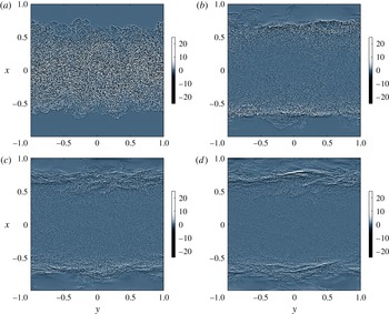
Numerical shadowgrams for the case with an initially linear stratification at (a)
 $t=20$
, (b)
 $t=40$
, (c)
 $t=60$
, (d)
 $t=80$
. This plot is of the two-dimensional Laplacian of mean projected density. As the problem is specified in dimensionless units, the colour scale is also dimensionless: if the domain were scaled into dimensional units using a factor
 $L$
, the values in the colour map would scale as
 $L^{-2}$
. The colour map values would also scale linearly with material density.

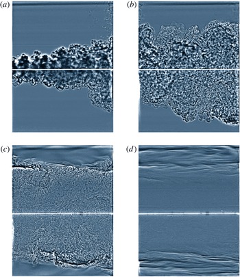
Experimental shadowgrams for linear stratification at (a)
 $t=5~\text{s}$
, (b)
 $t=10~\text{s}$
, (c)
 $t=20~\text{s}$
, (d)
 $t=80~\text{s}$
, from Davies Wykes & Dalziel (Reference Davies Wykes and Dalziel2014) with permission. The experimental time scales can be related to the dimensionless scales used here by dividing them by
 $\unicode[STIX]{x1D70F}=0.302H/(Ag)^{1/2}=0.254~\text{s}$
, where
 $2H$
is the total height of the tank and
 $A$
is the Atwood number in the experiment, although we have not attempted to match the level of initial perturbations which would be expected to influence this comparison. Frame (c) of this plot, at an experimental time of
 $t=20~\text{s}$
, i.e.
 $t/\unicode[STIX]{x1D70F}\simeq 80$
, corresponds to a dimensionless time close to that shown in figure 1(d).

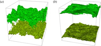
Passive scalar 0.1 % and 99.9 % surfaces at (a)
 $t=20$
, (b)
 $t=80$
.

3 Results
We will initially present some general properties of the calculations which we have performed to illustrate their overall agreement with the flows found in experiment. Synthetic shadowgram images can be calculated using the two-dimensional Laplacian of the column density through the simulation, see figure 1. As is often the case in experiments, these are informative about the qualitative aspects of the flow. The structure at early times, figure 1(a), looks much as would be expected for a canonical Rayleigh–Taylor mixing layer. However, at intermediate times, e.g. figure 1(c), some buoyant plumes are seen to be driven from the mixing layer. As time progresses, the density structure within the mixing layer becomes more uniform, but the transition at the surface of the mixing layer becomes sharper. These can be compared to the shadowgrams measured experimentally by Davies Wykes & Dalziel (Reference Davies Wykes and Dalziel2014), reproduced here as figure 2.
The effects of internal waves are seen at late time, in the movement of the surface of the mixing layer and the long-wavelength density modulations beyond its boundary. As these waves collide, localized plumes of material are driven into the stably stratified material outside the mixing layer, as can be seen in figure 1(c). The sharp density stratifications seen in figure 1(d) appear to be generated as these plumes fall back into the mixing layer. As found by Davies Wykes & Dalziel (Reference Davies Wykes and Dalziel2014), the internal waves can cause problems in distinguishing whether the density and velocity fluctuations which continue to late time can be identified as irreversible mixing processes. The level of qualitative agreement between experiment and calculation is good throughout the time for which the calculations are presented in this paper, figure 2(a–c), although the smoother density field within the mixing layer in figure 2(d) suggests that by
 $t=80~\text{s}$
in the experiment viscosity has started to have a substantial effect.
In the calculations presented here, a mass-weighted scalar has also been used to tag the fluids on each side of the initial interface, so the statistical properties of this scalar field may be used as a direct measure of mixing between the materials in the upper and lower parts of the stratification. Isosurfaces of this advected scalar are shown in figure 3. At early times, figure 3(a), the isosurfaces at extreme values, which track the edge of the mixing layer, are convoluted, but they become much smoother as the flow relaxes at late times, figure 3(b), with the surface perturbations now being predominantly the result of long-wavelength internal waves.
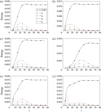
Energy budgets, in non-dimensional units corresponding to the values of
 $\unicode[STIX]{x1D70C}$
,
 $g$
and domain size specified in § 2.1. The plots are shown for (a) double linear, (b) symmetric quadratic, (c) asymmetric quadratic, (d) truncated double linear, (e) double linear with long-wavelength perturbation, (f) double linear with larger long-wavelength perturbation. Here
 $k_{x}$
is the vertical component of turbulence kinetic energy and
 $k_{y}$
,
 $k_{z}$
the two components in the horizontal plane, while
 $|\unicode[STIX]{x0394}\unicode[STIX]{x1D6F7}|$
is the magnitude of the change in potential energy. Scaling to typical dimensional values
 $\unicode[STIX]{x1D70C}^{\prime }=\unicode[STIX]{x1D70C}\times 10^{3}~\text{kg}~\text{m}^{-3}$
,
 $H^{\prime }=H\times 0.1~\text{m}$
and
 $g^{\prime }=g\times 10~\text{m}~\text{s}^{-2}$
, the time and energy axes here would be in units of
 $0.1~\text{s}$
and J, respectively.

Development of mean density at each height. (a) Double linear, (b) symmetric quadratic, (c) asymmetric quadratic, (d) truncated double linear, (e) double linear with long-wavelength perturbation, (f) double linear with larger long-wavelength perturbation.

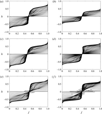
Development of mean tracer at each height. (a) Double linear, (b) symmetric quadratic, (c) asymmetric quadratic, (d) truncated double linear, (e) double linear with long-wavelength perturbation, (f) double linear with larger long-wavelength perturbation.

In figure 4, we compare the energy budget for a selection of initial configurations. In this diagram,
 $k$
is the total turbulent kinetic energy, while
 $k_{x}$
,
 $k_{y}$
and
 $k_{z}$
are the contributions to it from the
 $x$
,
 $y$
and
 $z$
directions.
 $|\unicode[STIX]{x0394}\unicode[STIX]{x1D6F7}|$
is the magnitude of the change in potential energy (so initially
 $k\sim |\unicode[STIX]{x0394}\unicode[STIX]{x1D6F7}|$
). The energy budgets for the linear and asymmetric stratifications, figure 4(a,c), appear very similar: the rate at which turbulent energy is produced in the mixing region is similar in each case. The symmetric stratification, figure 4(b), at first impression seems to have energy injected for a longer time, but while the turbulence kinetic energy peak is broader, it is also substantially lower and reduces sooner. The truncated profile takes longer to grow to a lower peak value, due to its reduced maximum Atwood number, but is otherwise similar in form to the linear and asymmetric profiles. Adding a substantial long-wavelength component to the initial perturbation, figure 4(e,f), leads to a higher initial growth rate, with minimal dissipation (
 $k\simeq |\unicode[STIX]{x0394}\unicode[STIX]{x1D6F7}|$
), but also significantly reduces the later-time peak in
 $k$
which dominates the mixing process. Apart from these cases, the peak in
 $k$
is approximately one-third of the total loss of potential energy. In all cases, the initial growth is significantly inhomogeneous. If we take
 $k_{x}$
to correspond to the vertical component of the turbulence kinetic energy, and
 $k_{y}$
and
 $k_{z}$
the components within the plane, then initially
 $k_{x}\sim 2k_{y}$
, but at late time
 $k_{x}$
reduces to a similar, or even somewhat smaller, value that the turbulence kinetic energy in the plane. For the long-wavelength perturbed cases,
 $k_{x}\gg k_{y}>k_{z}$
at the earliest times due to the resolved perturbation, but the asymmetry in
 $k_{y}/k_{z}$
, and the enhanced inhomogeneity in
 $k_{x}/(k_{y}+k_{z})$
, is removed almost entirely by the time of the first peak in the turbulence kinetic energy.
In figure 5, we show the development of the mean density of the flow with time. In all cases, the density structure relaxes to a similar smooth profile at late time, with a very small amount of overshooting from the mixing region into the external stable stratification. Apart from in the cases with strong initial perturbations, figure 5(e,f), the mixing process proceeds smoothly when shown as a plane average.
In figure 6, we show the structure of the advected scalar variable for each of the initial conditions considered previously, averaged in planes perpendicular to the imposed gravity. We see that in all cases within the mixing layer, the material is close to ideally mixed at late time, with a minimal gradient in volume fraction, while the edges of the structure are rather sharp. While the sequence of data is not clear in these graphs as plotted, the gradient at the edge of the region becomes sharper with time, which must result from the loss of energy in internal waves (the presence of which leads to apparent mixing in plane-averaged data which is in fact reversible). At late time, the outermost parts of the mixing profile become increasingly confined, due to the damping of internal waves, but there is evidence of some smoothing of the edges of the well-mixed core, most strongly in the case of the double-linear profile where there is the most residual turbulence in the mixing layer, figure 6(a,c). The mean tracer level within the mixing layer is rather lower than 0.5 in the case of the asymmetric profile, figure 6(c), due to the different propagation of the mixing layer into each component. There is more evidence for wave-like structures proceeding across the tracer fraction profile in these plots than in figure 5, although again major structure is only seen for the strongly perturbed cases, and in those cases at early time. Close to the centre of the mixing layer, the tracer distribution is close to linear – apart from at the very earliest times for the cases with strong initial perturbations; the sharp edges to the mixing profile start to appear as a point of inflection in the profile when this linear distribution reaches the edges of the perfect mixing profile.
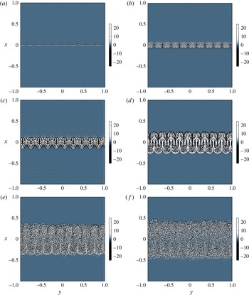
Numerical shadowgrams for the high-perturbation linear stratification at (a)
 $t=0$
, (b)
 $t=2$
, (c)
 $t=4$
, (d)
 $t=6$
, (e)
 $t=8$
, (f)
 $t=10$
. The colour scale is as in figure 1.

In figure 7, we show shadowgrams of the structure of the early time development of the case with a linear stratification and the higher amplitude regular initial surface perturbation. The perturbation initially grows in a form which reflects the
 $\unicode[STIX]{x1D706}=0.2$
periodicity of the macroscopic perturbation, but eventually suffers a rather rapid break down to turbulent structures. For the particular form of perturbation used, this breakdown appears to happen at caustics in the leading bubbles between
 $t=4$
and
 $t=6$
, figure 7(c,d). By
 $t=10$
, figure 7(f), there is very little evidence of the initial periodic structure. Comparing with figure 4, this might be expected, since around this time the velocity fluctuation in the flow has reduced significantly, and the anisotropy has reached a level more characteristic of flows with no macroscopic perturbation. This behaviour is interesting in the context of the concerns about double counting of macroscopic perturbations in turbulence models.
4 Late-time mixing layer structure
In this section, we develop a simple model for the internal structure of the mixing layer, based on thermodynamic concepts, and compare it with the results of our hydrodynamic calculations.
4.1 Probability density function
The probability density function (p.d.f.) of the initial profile is
 $$\begin{eqnarray}f_{0}(\unicode[STIX]{x1D70C})=\int \unicode[STIX]{x1D6FF}(\unicode[STIX]{x1D70C}_{0}(\boldsymbol{x})-\unicode[STIX]{x1D70C})\,\text{d}V.\end{eqnarray}$$
The sorted profile satisfies
 $$\begin{eqnarray}A\frac{\text{d}h_{s}}{\text{d}\unicode[STIX]{x1D70C}}=f_{0}(\unicode[STIX]{x1D70C}),\end{eqnarray}$$
where we use
 $h_{s}$
for the height corresponding to each density in the sorted profile and
 $A$
for the transverse area of the domain. Hence
 $$\begin{eqnarray}Ah_{s}(\unicode[STIX]{x1D70C})=\int _{0}^{\unicode[STIX]{x1D70C}}f_{0}(\unicode[STIX]{x1D70C}^{\prime })\,\text{d}\unicode[STIX]{x1D70C}^{\prime }.\end{eqnarray}$$
The sorted profile is monotonic, so
 $h_{s}(\unicode[STIX]{x1D70C})$
can be inverted uniquely to give
 $\unicode[STIX]{x1D70C}_{s}(h)$
.
If we specialise to initial profiles with a single unstable interface at
 $h_{i}$
, then within the sorted mixing layer
 $$\begin{eqnarray}h_{s}(\unicode[STIX]{x1D70C})=h_{{<}}(\unicode[STIX]{x1D70C})+h_{{>}}(\unicode[STIX]{x1D70C})-h_{i},\end{eqnarray}$$
where
 $h_{{<}}(\unicode[STIX]{x1D70C})$
and
 $h_{{>}}(\unicode[STIX]{x1D70C})$
are the height profiles either side of the interface, which are stable and hence invertible, and at the edges of the mixing layer
 $$\begin{eqnarray}\displaystyle & \displaystyle \unicode[STIX]{x1D70C}_{0}(h_{1})=\unicode[STIX]{x1D70C}_{0}(h)_{h\rightarrow h_{i},-}, & \displaystyle\end{eqnarray}$$
 $$\begin{eqnarray}\displaystyle & \displaystyle \unicode[STIX]{x1D70C}_{0}(h_{2})=\unicode[STIX]{x1D70C}_{0}(h)_{h\rightarrow h_{i},+}. & \displaystyle\end{eqnarray}$$
4.2 Variational model
In this section, we develop a variational formalism for the structure in the relaxed mixing layer inspired by the work of Lynden-Bell (Reference Lynden-Bell1967) and Tremaine, Hénon & Lynden-Bell (Reference Tremaine, Hénon and Lynden-Bell1986) on the equilibrium of stellar dynamical systems. These papers treated the solution of the equilibrium problem as an entropy maximization problem subject to constraints, as is also discussed in a different context by, e.g. Coolen, Kühn & Sollich (Reference Coolen, Kühn and Sollich2005), Chap. 13. Related approaches have been used before to study the vorticity field, (Carnevale, Frisch & Salmon Reference Carnevale, Frisch and Salmon1981; Montgomery Reference Montgomery, Ray Smith and Grandy1985; Robert & Sommeria Reference Robert and Sommeria1991). This has proved most useful for two dimensional turbulence and its analogues, as the non-uniqueness of the representation in terms of point vortices led to fundamental difficulties when applied in three dimensions (Robert & Sommeria Reference Robert and Sommeria1991). In the present case, the density stratification of the flow provides an alternative functional space in which we can apply this type of method.
In the present case, the probability density function is the volume occupied by material at each density, rather than the mass per unit volume in a six-dimensional phase space (with spatial and velocity coordinates). However, in both cases, the phase space variable is conserved in the absence of mixing processes. For the Vlasov equation applicable to stellar dynamics,
 $$\begin{eqnarray}\frac{\unicode[STIX]{x2202}f_{p}}{\unicode[STIX]{x2202}t}+\boldsymbol{v}\boldsymbol{\cdot }\unicode[STIX]{x1D735}f_{p}+\boldsymbol{a}\boldsymbol{\cdot }\unicode[STIX]{x1D735}_{\boldsymbol{v}}f_{p}=0,\end{eqnarray}$$
with
 $\boldsymbol{v}$
the velocity,
 $\boldsymbol{a}$
the acceleration due to body forces,
 $\unicode[STIX]{x1D735}$
the spatial vector derivative and
 $$\begin{eqnarray}\unicode[STIX]{x1D735}_{\boldsymbol{v}}=\left(\frac{\unicode[STIX]{x2202}}{\unicode[STIX]{x2202}v_{x}},\frac{\unicode[STIX]{x2202}}{\unicode[STIX]{x2202}v_{y}},\frac{\unicode[STIX]{x2202}}{\unicode[STIX]{x2202}v_{z}}\right),\end{eqnarray}$$
this implies that the phase space density,
 $f_{p}$
, is conserved on a trajectory satisfying
 $$\begin{eqnarray}\frac{\text{d}\boldsymbol{x}}{\text{d}t}=\boldsymbol{v};\quad \frac{\text{d}\boldsymbol{v}}{\text{d}t}=\boldsymbol{a}.\end{eqnarray}$$
In a similar manner, the mass conservation equation for incompressible flow
 $$\begin{eqnarray}\frac{\unicode[STIX]{x2202}\unicode[STIX]{x1D70C}}{\unicode[STIX]{x2202}t}+\boldsymbol{v}\boldsymbol{\cdot }\unicode[STIX]{x1D735}\unicode[STIX]{x1D70C}=-\unicode[STIX]{x1D70C}\unicode[STIX]{x1D735}\boldsymbol{\cdot }\boldsymbol{v}=0\end{eqnarray}$$
corresponds to conservation of density on a trajectory
 $\dot{\boldsymbol{x}}=\boldsymbol{v}$
from an initial position
 $\boldsymbol{x}=\boldsymbol{x}_{0}$
at
 $t=0$
. (For compressible flow in the absence of dissipation or shocks, a similar relation holds for the specific entropy of the fluid.)
The density p.d.f. at any time may in principle be calculated using
 $$\begin{eqnarray}f(\unicode[STIX]{x1D70C}_{1},t)=\int \unicode[STIX]{x1D6FF}(\unicode[STIX]{x1D70C}(\boldsymbol{x},t)-\unicode[STIX]{x1D70C}_{1})\,\text{d}^{3}\boldsymbol{x}.\end{eqnarray}$$
This probability density function corresponds to the volume occupied by material at each density,
 $$\begin{eqnarray}f(\unicode[STIX]{x1D70C})\,\text{d}\unicode[STIX]{x1D70C}=A\,\text{d}h=\text{d}V.\end{eqnarray}$$
In the absence of mixing and as a result of incompressibility,
 $\unicode[STIX]{x1D70C}(\boldsymbol{x},t)=\unicode[STIX]{x1D70C}(\boldsymbol{x}_{0},0)$
, and the Jacobian
 $\det (\unicode[STIX]{x2202}\boldsymbol{x}/\unicode[STIX]{x2202}\boldsymbol{x}_{0})=1$
, so that
 $f(\unicode[STIX]{x1D70C},t)=f(\unicode[STIX]{x1D70C}_{1},0)$
. However, coarse graining in the evaluation of
 $f$
– or, in reality, fine-scale diffusive processes once the transport of material has led to different densities becoming finely intermingled – will mean that the p.d.f. can in fact change as a result of mixing (Lynden-Bell Reference Lynden-Bell1967).
Applying the formalism of Lynden-Bell (Reference Lynden-Bell1967) to the current problem, we define a variational integral
 $$\begin{eqnarray}I=A\int \frac{\text{d}h}{\text{d}\unicode[STIX]{x1D70C}}\left(\ln \frac{\text{d}h}{\text{d}\unicode[STIX]{x1D70C}}+\unicode[STIX]{x1D706}\unicode[STIX]{x1D70C}+\unicode[STIX]{x1D707}\unicode[STIX]{x1D70C}h\right)\text{d}\unicode[STIX]{x1D70C}.\end{eqnarray}$$
The first term is a configurational entropy in the form derived by Shannon (Reference Shannon1948),
 $f\ln f$
, to within a constant term which plays no role in the eventual solution, where
 $f$
is given in terms of the density distribution by (4.12). The integral
 $\int f(\unicode[STIX]{x1D70C})\ln f(\unicode[STIX]{x1D70C})\,\text{d}\unicode[STIX]{x1D70C}$
will increase monotonically with time as a result of mixing processes. In the absence of other constraints, the variational maximum of this function will lead to a uniform density distribution. In statistical physics, a function of this form was proposed by Boltzmann when formulating his H-theorem, dependent on the phase space density
 $f(\boldsymbol{x},\boldsymbol{v},t)$
(Boltzmann Reference Boltzmann1964). For the nearly incompressible flow treated in the present paper, we have marginalized the probability density function to be a function of the local fluid density,
 $f(\unicode[STIX]{x1D70C},t)$
.
The Lagrange multipliers
 $\unicode[STIX]{x1D706}$
and
 $\unicode[STIX]{x1D707}$
are used to impose constant mass
 $$\begin{eqnarray}M=\int \unicode[STIX]{x1D70C}\,\text{d}V\end{eqnarray}$$
and potential energy
 $$\begin{eqnarray}\unicode[STIX]{x1D6F7}=\int \unicode[STIX]{x1D70C}gh\,\text{d}V,\end{eqnarray}$$
respectively. It is appropriate to require the potential energy to be constant, as we are interested in the structure of an equilibrium profile, and so by the principle of virtual work all relevant variations must release no further potential energy. There seems to be a natural relation between the physical interchange of fluid parcels during turbulent mixing and the infinitesimal interchanges which are modelled by the functional variation.
The configurational entropy term corresponds to a net attraction towards statistically well-represented states within the ensemble of possible configurations. The logarithmic form chosen used here is standard in statistical physics, and does not require a characteristic scale to be defined for the density, if that is assumed to be strictly positive. Any direct relationship to the physical entropy is, however, obscured by the incompressible limit we are assuming, where the sound speed is assumed to be very large compared to any scale of interest.
Note that the integrals in (4.13) may be transformed between integrals over position and integrals over density because the stability of the equilibrium profile to interchange instability implies that the function
 $h(\unicode[STIX]{x1D70C})$
is monotonic.
Varying
 $h(\unicode[STIX]{x1D70C})\rightarrow h+\unicode[STIX]{x1D6FF}h$
gives
 $$\begin{eqnarray}\unicode[STIX]{x1D6FF}I=\int \left(1+\ln \frac{\text{d}h}{\text{d}\unicode[STIX]{x1D70C}}+\unicode[STIX]{x1D706}\unicode[STIX]{x1D70C}+\unicode[STIX]{x1D707}\unicode[STIX]{x1D70C}h\right)\frac{\text{d}\unicode[STIX]{x1D6FF}h}{\text{d}\unicode[STIX]{x1D70C}}+\unicode[STIX]{x1D707}\unicode[STIX]{x1D70C}\frac{\text{d}h}{\text{d}\unicode[STIX]{x1D70C}}\unicode[STIX]{x1D6FF}h\,\text{d}\unicode[STIX]{x1D70C},\end{eqnarray}$$
where the functional extremum of
 $I$
satisfies
 $\unicode[STIX]{x1D6FF}I=0$
. Integrating the first component by parts subject to boundary conditions gives
 $$\begin{eqnarray}\unicode[STIX]{x1D6FF}I=-\int \left(\frac{\text{d}^{2}h}{\text{d}\unicode[STIX]{x1D70C}^{2}}\left/\frac{\text{d}h}{\text{d}\unicode[STIX]{x1D70C}}\right.+\unicode[STIX]{x1D706}+\unicode[STIX]{x1D707}h\right)\unicode[STIX]{x1D6FF}h\,\text{d}\unicode[STIX]{x1D70C},\end{eqnarray}$$
so that either
 $\unicode[STIX]{x1D6FF}h=0$
and the initial solution is unperturbed, or
 $$\begin{eqnarray}\frac{\text{d}^{2}h}{\text{d}\unicode[STIX]{x1D70C}^{2}}+(\unicode[STIX]{x1D706}+\unicode[STIX]{x1D707}h)\frac{\text{d}h}{\text{d}\unicode[STIX]{x1D70C}}=0.\end{eqnarray}$$
This equation can be integrated once to give
 $$\begin{eqnarray}\frac{\text{d}h}{\text{d}\unicode[STIX]{x1D70C}}+\unicode[STIX]{x1D706}h+\frac{\unicode[STIX]{x1D707}}{2}h^{2}=\text{const.},\end{eqnarray}$$
and again to give the equilibrium density profile in implicit form as
 $$\begin{eqnarray}\unicode[STIX]{x1D707}h=2\unicode[STIX]{x1D705}\tanh \unicode[STIX]{x1D705}(\unicode[STIX]{x1D70C}-\unicode[STIX]{x1D70C}^{\star })-\unicode[STIX]{x1D706},\end{eqnarray}$$
a simple, universal prediction for the density profile across the mixing zone. Note that without the potential energy constraint,
 $\unicode[STIX]{x1D707}\rightarrow 0$
, the variational solution is
 $$\begin{eqnarray}f(\unicode[STIX]{x1D70C})\propto \unicode[STIX]{x1D6FF}(\unicode[STIX]{x1D70C}-\unicode[STIX]{x1D70C}^{\star }),\end{eqnarray}$$
i.e. the density becomes uniform, as expected.
This leaves four as-yet free parameters
 $\unicode[STIX]{x1D706}$
,
 $\unicode[STIX]{x1D707}$
,
 $\unicode[STIX]{x1D70C}^{\star }$
and
 $\unicode[STIX]{x1D705}$
, which determine the position of the inflection point of the profile in height and density, the width and maximum slope of the profile. Two of these parameters may be determined by requiring the density profile to match the initial profile at the edges of the mixing region
 $h_{1}$
and
 $h_{2}$
 $$\begin{eqnarray}\displaystyle & \displaystyle \unicode[STIX]{x1D70C}(h_{1})=\unicode[STIX]{x1D70C}_{0}(h_{1}), & \displaystyle\end{eqnarray}$$
 $$\begin{eqnarray}\displaystyle & \displaystyle \unicode[STIX]{x1D70C}(h_{2})=\unicode[STIX]{x1D70C}_{0}(h_{2}), & \displaystyle\end{eqnarray}$$
 $\unicode[STIX]{x1D70C}_{0}(h)$
is the initial density profile. While these nonlinear equations may have multiple solutions, many of these may be eliminated by the requirement that at the edge of the mixing layer, the gradient of the mixed profile must be larger than that of the unmixed profile, as entrainment tends to move the density of the material towards the perfectly mixed density.
A third parameter is determined by requiring that the mass within the mixing region is conserved,
 $$\begin{eqnarray}\int _{h_{1}}^{h_{2}}\unicode[STIX]{x1D70C}_{0}\,\text{d}h=\int _{h_{1}}^{h_{2}}\unicode[STIX]{x1D70C}\,\text{d}h.\end{eqnarray}$$
Here the integral over the model for the final profile may be performed analytically
 $$\begin{eqnarray}\displaystyle \int _{h_{1}}^{h_{2}}\unicode[STIX]{x1D70C}\,\text{d}h & = & \displaystyle \frac{2\unicode[STIX]{x1D705}^{2}}{\unicode[STIX]{x1D707}}\int _{\unicode[STIX]{x1D70C}_{0}(h_{1})}^{\unicode[STIX]{x1D70C}_{0}(h_{2})}\frac{\unicode[STIX]{x1D70C}}{\cosh ^{2}\unicode[STIX]{x1D705}(\unicode[STIX]{x1D70C}-\unicode[STIX]{x1D70C}^{\star })}\,\text{d}\unicode[STIX]{x1D70C}\nonumber\\ \displaystyle & = & \displaystyle \frac{2}{\unicode[STIX]{x1D707}}[\unicode[STIX]{x1D705}\unicode[STIX]{x1D70C}\tanh \unicode[STIX]{x1D705}(\unicode[STIX]{x1D70C}-\unicode[STIX]{x1D70C}^{\star })-\ln \cosh \unicode[STIX]{x1D705}(\unicode[STIX]{x1D70C}-\unicode[STIX]{x1D70C}^{\star })]_{\unicode[STIX]{x1D70C}_{0}(h_{1})}^{\unicode[STIX]{x1D70C}_{0}(h_{2})}.\end{eqnarray}$$
These give three equations constraining the form of the mixing layer based on the structure of the initial solution.
For this model, the remaining parameter is the only way in which the internal structure within the final mixing layer can depend on the structure of the initial stratification. If the dissipation of the convectively released kinetic energy were perfect, then
 $\unicode[STIX]{x1D705}\rightarrow 0$
, and the value of
 $\unicode[STIX]{x1D70C}_{0}(h_{1})=\unicode[STIX]{x1D70C}_{0}(h_{2})=\unicode[STIX]{x1D70C}^{\star }$
is determined by the mass conservation constraint
 $$\begin{eqnarray}\int _{h_{1}}^{h_{2}}\unicode[STIX]{x1D70C}\,\text{d}h=\unicode[STIX]{x1D70C}^{\star }(h_{2}-h_{1}).\end{eqnarray}$$
This is the perfect mixing profile of Davies Wykes & Dalziel (Reference Davies Wykes and Dalziel2014). Hence the remaining parameter is effectively a measure of how efficiently the mixing process dissipates energy, rather than using it to reorder stably stratified parts of the density profile.
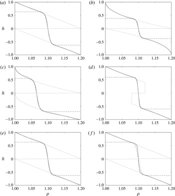
Model comparison: dotted is initial state, solid is final state, dashed is model fit. (a) Double linear, (b) symmetric quadratic, (c) asymmetric quadratic, (d) truncated double linear, (e) double linear with long-wavelength perturbation, (f) double linear with larger long-wavelength perturbation. The model parameters have been chosen to give a good fit to the mixing layer profile in (a–d). In (e) and (f), the fit has been kept as that shown in (a), to make it easier to compare these panels, however it should be clear that by reducing energy overshoot, the model can be fit to the density profiles from the TURMOIL calculations at a similar accuracy to the other cases.

4.3 Comparison with results
In figure 8, we compare the densities found at the final time step for each of the initial density profiles we consider, shown as a solid curve, with the tanh-profile form predicted by the variational model, shown as a dashed curve. The agreement between these profiles is generally very good, apart from the furthest extrema of the overshoot in the mixing layer. The fit has not been adjusted for the final two profiles, with the enhanced initial perturbations: while it seems clear that an improved tanh-profile fit could be obtained, including the fit tuned to the case shown in figure 8(a) serves as a useful datum for the reduced level of overshoot found in these cases.
The profiles for which calculations have been performed have been chosen to address the obvious questions which arose when the good agreement of the variational formula with the simple two-linear profile was observed: is the form robust to changes in the source of buoyancy and boundary conditions of final mixing layer as a result of density stratification, figure 8(b,d), surface perturbations, figure 8(e,f) or the symmetry of the initial conditions, figure 8(c). In each case, the prediction of the simple formula for the structure of the final mixing layer appears to be robust, subject only to changes in the total extent of the mixing layer which is an undetermined constant in the model (so long as the calculations are run with sufficient numerical resolution to well resolve the final mixing layer). There is a small amount of mixing beyond the extent of layer predicted by the model, which corresponds to a blurring of the sharp change in gradient predicted at the edge of the mixing region. However, this appears to result from the late-time effects of internal waves and anisotropic turbulence in the stratified envelope, once the nearly isotropic turbulence within the mixing layer itself has died down. There is other evidence in the distribution of the scalar variable within the mixing layer, figure 6, and the structure of the edge of the mixing layer observed at mid to late times in experimental and calculational shadowgraphy data, figures 1 and 2, that this sharp edge does reflect a physical reality.
5 Discussion and conclusions
We have studied the properties of stratification-bounded mixing layers, developing a simple model for the late-time density stratification within the mixing layer.
The model discussed in § 4.2 does a good job of matching the late-time structure of the mixing layers, for each of the stratification-bounded flows which we consider here. It is based on a simple application of concepts from statistical physics. The constrained variational procedure which is used to derive the theoretical profile seems to have some underlying similarity to the interchange of material by turbulent eddies which causes the mixing in reality. It does not fully capture the extent of overshooting seen at the very edge of the layer, which may be a result of the different nature of mixing driven by internal waves and highly anisotropic turbulence in the stably stratified regime.
The results of these calculations may also be compared to the potential temperature measurements in the troposphere, which also tend to the structure of tanh-like regions with near-neutral stability with intervening, strongly stable temperature inversions (Reible Reference Reible1998). One might then consider the near-neutral stability regions as the fossils of previous episodes of convective instability, of whatever origin. The experiments and calculations also show the internal waves and sharp lamina found in radar sounding of the troposphere (Gossard, Jensen & Richter Reference Gossard, Jensen and Richter1971).
This approach may be compared to previous studies where the use of maximization of dissipation as a principle for isolating dynamic equilibria of turbulent flows has been explored (Malkus Reference Malkus1956; Bertram Reference Bertram2015), which can be related to similar approaches used more widely in non-equilibrium physics (Onsager Reference Onsager1931a ,Reference Onsager b ; Jaynes Reference Jaynes1957a ,Reference Jaynes b ; Prigogine Reference Prigogine1962; Dewar Reference Dewar2005).
This is in contrast to the well-known failure of Gaussian statistics to capture all the properties of evolving turbulence (Thornber, Mosedale & Drikakis Reference Thornber, Mosedale and Drikakis2007). However, it is likely that the impact of intermittency will be reducing with time as the mixing layers relax to equilibrium, so this is perhaps not that surprising. Given that the model agrees well for the relaxed limit, it is possible that studying the convergence to this limit may provide additional insights towards a statistical model of fully turbulent flows.
Acknowledgements
This work has benefited from many discussions with C. Batha, S. Dalziel, M. Davies Wykes, A. Lawrie, P. Moresco and D. Youngs.