2.1 SATES turbulence modeling method

It should be noted that the SATES method used in the present study is the model developed recently [Reference Han and Krajnović21, Reference Han and Krajnović22, Reference Han and Krajnović30, Reference Xia, Cheng, Han and Mao31] and previously the VLES method. It should be noted that Pope classifies turbulence models [Reference Pope32] and the VLES corresponds to ‘the filter and grid are too coarse to resolve 80% of the energy’. However, nearly all of the numerical calculation results of the SATES method developed by Han et al. [Reference Han and Krajnović21, Reference Han and Krajnović22, Reference Han and Krajnović30, Reference Xia, Cheng, Han and Mao31] show that the turbulent kinetic energy directly solved is larger than 90% even on a coarse grid. That is, the VLES developed by Han et al. [Reference Han and Krajnović21, Reference Han and Krajnović22, Reference Han and Krajnović30, Reference Xia, Cheng, Han and Mao31] is fundamentally different from the VLES method defined by Pope. In fact, the performance is very similar to the traditional LES method. Based on these, in the following investigation, this study refers to the turbulence model developed in the early stage as the SATES method.

In the present numerical simulations, the SATES modeling is based on baseline (BSL) k-ω turbulence model proposed by Menter [Reference Menter33], which retains the robust and accurate formulation of the Wilcox k-ω model in the near wall region and takes advantage of the freestream independence of the k- $\varepsilon$ model in the outer part of the boundary layer. In the SATES modeling, the transport equations for the modeled turbulent kinetic energy, k, and the specific dissipation rate, ω, are exactly the same as in the BSL k-ω turbulence model [Reference Menter33], given by

(1) \begin{align}\frac{{D\rho k}}{{Dt}} &= {\tau _{ij}}\frac{{\partial {u_i}}}{{\partial {x_j}}} - \beta _1^*\rho \omega k + \frac{\partial }{{\partial {x_j}}}\left[ {\left( {\mu + {\sigma _k}{\mu _t}} \right)\frac{{\partial k}}{{\partial {x_j}}}} \right] \end{align}

(2) \begin{align}\frac{{D\rho \omega }}{{Dt}} &= \omega \bigg(\frac{\gamma }{k}{\tau _{ij}}\frac{{\partial {u_i}}}{{\partial {x_j}}} - \beta \rho \omega \bigg) + \frac{\partial }{{\partial {x_j}}}\left[ {\left( {\mu + {\sigma _\omega }{\mu _t}} \right)\frac{{\partial \omega }}{{\partial {x_j}}}} \right] + 2\rho \left( {1 - {F_1}} \right){\sigma _{\omega 2}}\frac{1}{\omega }\frac{{\partial k}}{{\partial {x_j}}}\frac{{\partial \omega }}{{\partial {x_j}}} \\[8pt]\nonumber\end{align}

where F ₁ is designed to be one in the near wall region (activating the original model) and zero away from the surface. More details can be found in Ref. (Reference Menter33).

The constants $\phi$ of BSL k-ω turbulence model are calculated from the constants, $\phi$ ₁ , $\phi$ ₂ , as follows:

(3) \begin{align}\phi = {F_{\rm{1}}}{\phi _{\rm{1}}}{\rm{ + }}\left( {{\rm{1 - }}{F_{\rm{1}}}} \right){\phi _{\rm{2}}} \end{align}

where $\phi$ ₁ and $\phi$ ₂ represent any constant in the Wilcox k-ω model ( ${\sigma _{k1}}, \ldots $ ) and k- $\varepsilon$ model ( ${\sigma _{k2}}, \ldots $ ).

Compared to the BSL k-ω model, the SATES based on BSL k-ω model only modifies the formulation of turbulent viscosity, in the form of

(4) \begin{align}{\mu _t} = {F_r}\rho k/\omega \end{align}

where F _r is the resolution control function, and its formulation is the key issue of SATES modeling. Compared with DES method [Reference Strelets34], SATES behaves seamless transition from URANS to LES in separated flow, such as backstep flow and flow past bluff body [Reference Han and Krajnović22]. Due to the difference between the transition between URANS and LES, the SATES method shows much weaker log-law mismatch compared with DES, which is a common problem in hybrid RANS-LES method. Another advantage of SATES is that it can achieve quicker transition from URANS to LES compared to DES, which affects a lot in convective heat transfer and combustion simulations. In SATES method, only partial URANS modeling works in the simulation, which is decided by the proportion of modeled turbulent kinetic energy to the total turbulent kinetic energy. The modeled and total turbulent kinetic energy are computed by turbulent energy spectrum, with the form of [Reference Han and Krajnović30]

(5) \begin{align}{F_r} = \frac{{{k_{\left( {{L_k} \to {L_c}} \right)}}}}{{{k_{\left( {{L_k} \to {L_i}} \right)}}}} = \frac{{\frac{1}{2}{\tau _{ii\left( {{L_k} \to {L_c}} \right)}}}}{{\frac{1}{2}{\tau _{ii\left( {{L_k} \to {L_i}} \right)}}}}{\rm{ = }}\frac{{{{\left[ {1.0 - \exp \left( { - {\beta ^ * }{L_c}/{L_k}} \right)} \right]}^n}\tau _{ij}^{{\rm{RANS}}}}}{{{{\left[ {1.0 - \exp \left( { - {\beta ^ * }{L_i}/{L_k}} \right)} \right]}^n}\tau _{ij}^{{\rm{RANS}}}}}\nonumber \\\mathop { = = = = = = }\limits_{0 \le {F_r} \le 1}^{{\rm{physical}}\,{\rm{limit}}} \min \left( {1.0,{{\left[ {\frac{{1.0 - \exp \left( { - {\beta ^ * }{L_c}/{L_k}} \right)}}{{1.0 - \exp \left( { - {\beta ^ * }{L_i}/{L_k}} \right)}}} \right]}^n}} \right) \end{align}

where the function min (x, y) refers to the minimum value between x and y, and $\beta$ and n are the model constants. It can be seen that three turbulence length scales are involved in Equation (5), i.e., L _c , L _i , and L _k , which are the turbulent cutoff length scale, integral length scale and Kolmogorov length scale, respectively, defined as

(6) \begin{align} \begin{array}{l}{L_c} = {C_x}{\left( {{\Delta _x}{\Delta _y}{\Delta _z}} \right)^{1/3}},\\{L_i} = {k^{3/2}}/(\beta _1^ * k\omega ),\\{L_k} = {\nu ^{3/4}}/{\left( {\beta _1^ * k\omega } \right)^{1/4}}\end{array} \end{align}

It should be noted that the relation of the dissipation rate and the specific dissipation rate is used in the formulation, i.e., $\varepsilon = \beta _1^ * k\omega $ . The model constant, ${C_x}$ , is related to the Smagorinsky LES model constant, ${C_s}$ , as

(7) \begin{align}{C_x} = \sqrt {0.3} {C_s}/\beta _1^ * \end{align}

where ${C_s} = 0.1$ is the Smagorinsky model constant in the present SATES model. All the model constant involved in Equations (1)–(7) are summarised in Table 1. More details can be obtained in the Refs. [Reference Han and Krajnović21, Reference Han and Krajnović30].

Table 1.

The model constants for the SATES BSL k-ω turbulence model

Actually, the derivation process of the model constant, C _x , is closely linked to the sub-grid stress model of traditional LES. In the literature [Reference Wenchang, Han, Min, Ma and Yan35], it has been demonstrated that the equivalence can be obtained between SGS stress and modeled Reynolds stress by introducing the resolution control function. To achieve LES mode, the turbulent viscosity is damped by the resolution control function:

(8) \begin{align}{\mu _{t,{\rm{SATES}}}} = {F_r}{\mu _{{\rm{RANS}}}}{\rm{ = }}\rho {C_\mu }{C_x}\Delta \sqrt k \end{align}

where $\Delta = {\left( {{\Delta _x}{\Delta _y}{\Delta _z}} \right)^{1/3}}$ . By introducing second assumption of equilibrium between turbulent kinetic energy production and dissipation, it can be obtained:

(9) \begin{align}{P_k} = {\mu _{t,\Delta }}{\left| S \right|^2} = \rho \varepsilon \end{align}

where ${P_k}$ and $\left| S \right| = \sqrt {2{S_{ij}}{S_{ij}}} $ are production of turbulent kinetic energy and strain rate, respectively.

Also, with another assumption of scale similarity, the empirical shear flow relation is:

(10) \begin{align}\left\langle {uv} \right\rangle \approx 0.3k\left| S \right| = \varepsilon \end{align}

Finally, the sub-filter is identical to the standard Smagorinsky-type LES model, and the sub-filter turbulent viscosity is:

(11) \begin{align}{\mu _t} = \rho {\left( {{C_s}\Delta } \right)^2}\left| S \right| \end{align}

and the model constant, C _x , is:

(12) \begin{align}{C_x} = \sqrt {0.3} {{{C_s}}/{{C_\mu }}} \end{align}

It can be seen that Equation (12) is the same as Equation (7). The model constant, C _s , has a typical value [Reference Canuto and Cheng36] between 0.08 and 0.22, and it is chosen to 0.1 in this study, resulting in ${C_x} = 0.61$ .

It can be seen that Equation (10) includes the assumption involving the parameter of strain rate. However, the computation of turbulent viscosity in the SST k-ω modeling includes the correction of strain rate. It would lead to a correction when using SST model as underlying RANS model in SATES method, which will be studied later. The turbulent viscosity computed by SATES-SST model has the formulation as following:

(13) \begin{align}\mu_{t}=F_{r}\rho\frac{k}{\max(w,|S|F_2/a_1)},F_{2}=\text{tanh}\left[(\text{arg}_{1})^2\right],\text{arg}_1=\max\left(\frac{2\sqrt{k}}{\beta_{1}^{*}\omega d},\frac{500}{\omega d^{2}}\right) \end{align}

Here, the SATES-BSL and SATES-SST models were tested in the turbulent channel flow at Re _τ =1,000. Figures 1 and 2 show the results of two different models. It can be seen that the results of velocity and Reynolds stress components show small differences while the resolution control function shows relative large discrepancies in the distribution along the wall normal direction. The SATES-BSL model maintain at a certain level in the log-law region, while SATES-SST model gradually decreases with increasing the wall distance, which may result from the involvement of strain rate in the turbulent modeling.

Figure 1.

Comparisons of mean streamwise velocity profile and turbulent variables at turbulent channel flow.

Figure 2.

Reynolds stress components profile predicted by different SATES models at turbulent channel flow.

2.2 Weighted compact nonlinear schemes

In the current high-order accurate simulations, a fourth-order accurate WCNS is used for discretisation of convection term. Here, we introduce the WCNS scheme by using one-dimensional inviscid flux discretisation is considered for simplicity, let ${{{\boldsymbol{U}}}_j} = {{\boldsymbol{U}}}\left( {{x_j},t} \right),{x_j} = jh$

(14) \begin{align}\frac{{\partial {{\boldsymbol{U}}}}}{{\partial t}} + \frac{{\partial {{\boldsymbol{E}}}}}{{\partial x}} = 0 \end{align}

Equation (14) is discretised by using the finite differencing method, we obtain the semi-discrete approximation for the j ^th node:

(15) \begin{align}\left( \frac{\partial{{\boldsymbol{U}}}}{\partial t} \right)_{j} = - {{\boldsymbol{E}}}_{j}^{\prime}, \end{align}

In the WCNS schemes, three components are included in the WCNS schemes procedure, which are high-order flux difference, numerical flux evaluation, and weighted averaging interpolation. In the first component, the explicit high-order flux difference form is preferred, which is:

(16) \begin{align}{\boldsymbol{E}}_{j}^{\prime} = \frac{\alpha }{h} \left( \hat{{\boldsymbol{E}}}_{j + \frac{1}{2}} - \hat{{\boldsymbol{E}}}_{j - \frac{1}{2}} \right) + \frac{b}{h} \left( \hat{{\boldsymbol{E}}}_{j + \frac{3}{2}} - \hat{{\boldsymbol{E}}}_{j - \frac{3}{2}} \right) \end{align}

Where α = 9/8, b = −1/24, and Equation (16) is fourth-order in accuracy.

In the second component, numerical flux evaluation ${{\hat{{\boldsymbol{E}}}_{j \pm 1/2}}} = {{\boldsymbol{E}}}\left( {{\hat{{\boldsymbol{U}}}}_{j \pm 1/2}^L,{\hat{{\boldsymbol{U}}}}_{j \pm 1/2}^R} \right)$ could be computed by Roe’s, Steger-Warming’s, Van-Leer’s or other flux evaluation methods. In this work, Roe’s flux is used.

In the third component, nonlinear weighted averaging interpolation is used to get the variable ${\hat{ {\boldsymbol{U}}}}_{j \pm 1/2}^L$ and ${\hat{{\boldsymbol{U}}}}_{j \pm 1/2}^R$ , and only ${\hat{ {\boldsymbol{U}}}}_{j \pm 1/2}^L$ is considered for simplicity, which is:

(17) \begin{align}{\hat{{\boldsymbol{U}}}}_{j+1/2}^{L,5th} & = \sum^{2}_{k=0} {\omega _k} {\hat{{\boldsymbol{U}}}}_{j + 1/2}^{L,k,3th}, \nonumber\\{\hat{{\boldsymbol{U}}}}_{j + 1/2}^{L,0,3th} &= \left( 3{{\bf{U}}_{j - 2}} - 10{\bf{U}}_{j - 1} + 15{{\bf{U}}_j} \right)/8, \\[3pt]{\hat{{\boldsymbol{U}}}}_{j + 1/2}^{L,1,3th} &= \left( -{\bf{U}}_{j - 1} - 6{\bf{U}}_{j} + 3{\bf{U}}_{j+1}\ \right)/8,\nonumber \\[3pt]{\hat{{\boldsymbol{U}}}}_{j + 1/2}^{L,2,3th} &= \left( 3{{\bf{U}}_{j}} + 6{\bf{U}}_{j+1} + -{\bf{U}}{j+2}\ \right)/8.\nonumber\end{align}

The Z-type nonlinear weight [Reference Borges, Carmona, Costa and Don37] is used for ω _k in Equation (17). Considering the p ^th characteristic variables $u_{j }={\textbf{U}}_{j, p}$ , which has the following formulation:

(18) \begin{align}{\omega _k} = \frac{{{\alpha _k}}}{{\sum\limits_{l = 0}^2 {{\alpha _l}} }},{\alpha _k} = {C_k}\left( {1 + \frac{{{\tau _{\rm{5}}}}}{{{\beta _k} + \varepsilon }}} \right), for\ k = 0,1,2 \end{align}

Where the global smoothness indicator ${\tau _5} = \left| {{\beta _0} - {\beta _2}} \right|$ coefficients C _k , $\beta$ _k and $\varepsilon$ are computed by:

(19) \begin{align}\left( {{C_0},{C_1},{C_2}} \right) = \left( {\frac{1}{{16}},\frac{{10}}{{16}},\frac{5}{{16}}} \right),\left\{ {\begin{array}{*{20}{c}}{{\beta _0} = \frac{1}{4}{{\left( {{u_{j - 2}}{\rm{ - }}4{u_{j - 1}} {} {\rm{ + }}3{u_j}} \right)}^2} + {{\left( {{u_{j - 2}} - 2{u_{j - 1}} + {u_j}} \right)}^2},}\\{{\beta _1} = \frac{1}{4}{{\left( {{u_{j - 1}} - {u_{j + 1}}} \right)}^2} + {{\left( {{u_{j - 1}} - 2{u_j} + {u_{j + 1}}} \right)}^2},}\\{{\beta _2} = \frac{1}{4}{{\left( {3{u_j} - 4{u_{j + 1}} + {u_{j + 2}}} \right)}^2} + {{\left( {{u_j} - 2{u_{j + 1}} + {u_{j + 2}}} \right)}^2}.}\end{array}} \right. \end{align}

In the nonlinear weight, $\varepsilon$ = 10⁻⁴⁰ is recommended. However, the extra dissipation caused by nonlinear weight cannot ensure optimal order accuracy near critical points of smooth solutions. Two optional values of $\varepsilon$ are provided in the present study. The large value $\varepsilon$ = 100 (approaching to linear weight) is used to reduce numerical dissipation in the cases of subsonic flow and the small value $\varepsilon$ = 10⁻⁶ is used to capture the shock in the transonic flow. In addition, the viscous terms are solved by a fourth-order central differencing when the convection terms are solved by the WCNS scheme.

2.3 Solver

The present numerical simulations are carried out in a compressible solver called PHengLEI-HyOrder. The solver in a cell-central finite differencing formulation based on multi-block structured grids, which is applied to validate the SATES turbulence modeling method. The temporal term is discretised by a second-order backward differentiation, and implicit lower-upper symmetric Gauss-Seidel (LU-SGS) with Newton-like sub-iteration for time-integration when solving the NS and turbulence model equations. The computations of SATES start from the initial fields obtained by the steady RANS turbulence modeling.

3.1 Resolution control function

In the SATES turbulence modeling, the core parameter is the resolution control function F _r , which basically characterises the turbulence mode in the current turbulent modeling process, that is, the proportion of the modeled kinetic energy of the turbulent modeling is adaptively adjusted with the change of the turbulent length scale, i.e., L _c , L _i , and L _k at the local flow field. In order to verify the currently developed adaptive turbulence simulation module based on the PHengLEI-HyOrder solver, the instantaneous distribution of the resolution control function F _r in different test cases is given by taking the subsonic flow around a square cylinder and the transonic flow around a cylinder as a reference. The result is shown in Fig. 3. It can be seen that the distribution of F _r has a relatively obvious relationship with the turbulent flow field. In the turbulent wake behind the bluff body, F _r is significantly reduced, the proportion of modeled turbulent kinetic energy is reduced, and the turbulent resolution is increased. In addition, Fr has obvious dynamic change characteristics and can be adaptively adjusted according to the local flow field characteristics and grid resolution, which indicates the ability to adaptively solve the turbulent flow field.

Figure 3.

The distributions of resolution control function.

In the present CFD solver, the additional variable, F _r, is stored in the cell centre, and there is no communication between adjacent grids. However, the turbulent variables, k, and ω involved in computation of F _r can be communicated in each iteration. Thus, there are some discontinuities of F _r in Fig. 3 which is caused in the post-processing process. The distribution of turbulent kinetic energy and specific dissipation rate are shown in Fig. 4, and it can be seen that the distributions of both parameters are quite smooth.

Figure 4.

The distributions of turbulent variables.

3.2 Flow past a circular cylinder at $Re = 3.9 \times 10^{3},\, Ma=0.2 $

A classic case of a turbulent flow simulation verification is the flow around a cylinder Re = 3.9×10³, which exhibits complicated flow separation phenomena, shear layer separation and transition, large-scale vortex shedding, i.e. complex flow physics phenomena. The unstable reverse pressure gradient acting on the smooth surface causes the flow separation point on the surface of cylinder to fluctuate over time, which presents a significant challenge to the numerical scheme and turbulence model. There are also abundant numerical simulations [Reference Kravchenko and Moin23, Reference Parnaudeau, Carlier, Heitz and Lamballais38] and experimental results [Reference Parnaudeau, Carlier, Heitz and Lamballais38] available for reference.

In the present compressible simulations, the coordinate origin is located at the centre of the cylinder. The freestream is along the positive direction of the x-coordinate axis, and Mach number Ma =0.2, Reynolds number Re = 3.9×10³(based on the freestream velocity U ₀ and the diameter of circular cylinder D). The far-field boundary condition is 50D from the no slip wall of cylinder, the spanwise size is set 4D and a translational periodic condition is applied. Two computational grids are used for the check of grid sensitivity. Three computational grids were generated, with the coarse grid (m0) containing 139×180×32 points, the medium grid (m1) containing 200×260×32 points and the finer grid (m2) containing 200×260×48 points in circumferential, normal and axial direction, respectively. The height of the first layer cells in three grids are set to y ⁺ $\approx$ 1, 0.8, 0.5, respectively. The non-dimensional time-steps ΔtU ₀/D are set to 8×10⁻³,5×10⁻³ and 2.5×10⁻³ for grid m0, m1 and m2 to satisfy the CFL (Courant-Friedrichs-Lewy) number less than 1.0 in most regions. The simulations run over at least 200 flow units (D/U ₀) and the last 120 flow units are used for statistics.

Figure 5 shows the time-averaged velocity profiles in the wake predicted by the present high-order scheme-based SATES simulations. In Fig. 5(a), the prediction of the time-averaged streamwise velocity <U>/U ₀ along the centre line reflects the predicted length of the recirculation. The length of the recirculation predicted by the current numerical simulation is in good agreement with the experimental results [Reference Parnaudeau, Carlier, Heitz and Lamballais38]. Furthermore, regardless of the streamwise velocity or the lateral velocity, as shown in Fig. 5(b) and Fig. 5(c), the current numerical simulation is in good agreement with the experimental results [Reference Parnaudeau, Carlier, Heitz and Lamballais38] at three different positions in the wake (x/D = 1.06, 1.54, and 2.02), demonstrating that the prediction of the width of the recirculation region is also accurate. Besides, the results predicted by three different grids show good consistency.

Figure 5.

Time-averaged velocity profile in the wake.

Laminar shear layer separation is the first separation of the cylinder trailing edge in the subcritical Reynolds number region. Then, the shear layer eventually becomes unstable as the downstream grows, transition to turbulence and experiences alternating large-scale vortex shedding. A significant difficulty for high-precision turbulence modeling is the emergence of wake turbulence. Figure 6 shows the distributions of Reynolds normal stresses $\lt u^{\prime}u^{\prime} \gt,\ \lt v^{\prime}v^{\prime} \gt $ and Reynolds shear stresses $\lt u^{\prime}v^{\prime} \gt $ in the wake (x/D = 1.06, 1.54, and 2.02). It can be seen that the current numerical results are in good agreement with the avaiable experimental results and large eddy simulation results [Reference Parnaudeau, Carlier, Heitz and Lamballais38]. Because of the shear effect of the separated shear layer, which causes significant Reynolds normal stress and shear stress near the shear layers, the Reynolds normal stress $\lt u^{\prime}u^{\prime} \gt $ and shear stress $\lt u^{\prime}v^{\prime} \gt $ have obvious two peaks located in the shear layers. And the peak range widens as the downstream progresses because the shear layers gradually get thicker. But only one peak can be seen near y/D = 0 in the distributions of Reynolds normal stress $\lt v^{\prime}v^{\prime} \gt $ . And the peak value steadily rises with the growth of the shear layer downstream due to the increasing instability of the separated shear layer and the alternating shedding of large-scale vortices.

Figure 6.

Reynolds stresses profile in the wake.

The above results demonstrate that the current high-order WCNS scheme-based SATES can accurately present the development of the shear layer from the quantised results as well as predict the shape of the separation zone behind the cylinder and the internal quantised velocity distribution results.

3.3 Flow past a square cylinder at $Re = 2.2 \times 10^{4},\, Ma=0.2 $

The flow around a square cylinder is comparable to flow around a circular cylinder. The square cylinder differs in that the geometric discontinuities on the surface, leading to the fixed separation location. While the separation location of the flow around a circular cylinder is changeable by pressure gradient on the smooth surface. In this case, the coordinate origin is located at the centre of the cylinder. The freestream is along the positive direction of the x-coordinate axis, and Mach number Ma =0.2, Reynolds number Re = 2.2×10⁴ (based on the freestream velocity U ₀ and the diameter of circular cylinder D). The size of computational domain has 4D in spanwise direction and a translational periodic condition is applied. Upstream and downstream from the centre of square cylinder extends 10D and 20D, respectively. The vertical dimension of the channel is 14D and the blockage ratio is 7.1%, which is close to 7% in experiment of Lyn, Einav, Rodi and Park [Reference Lyn, Einav, Rodi and Park39]. Two different computational grids are generated to check the grid sensitivity, which the coarse grid (denoted as m1) contains about 1.5 million cells and the fine grid (denoted as m2) contains about 3.7 million cells, and the height of first cell is set to y ⁺≍1. The non-dimensional time-step ΔtU ₀/D is 5×10⁻³ and 2.5×10⁻³ for grid m1 and m2 to satisfy the CFL number less than 1.0. The simulations run over at least 300 flow units (D/U ₀) and the last 180 flow units are used for statistics.

Figure 7 shows the instantaneous flow field structure of the SATES numerical simulation under the two computational grids. The three-dimensional vortex structures are identified using the Q-criterion (Q(D/U ₀)² = 0.1) and coloured by strreamwise velocity U/U ₀. It can be seen that the current numerical simulation has well predicted the separation shear layer and transition in the leading-edge corner region. When it is further developed to mix with the trailing edge separation wake, alternating large-scale von-karman vortex shedding is formed and at the same time, obvious streamwise vortices are formed. It shows that the current high-order adaptive turbulence simulation has high resolution in capturing the instantaneous flow field.

Figure 7.

Three-domensinal vortex structures coloured by streamwise velocity (Q(D/U₀)² = 0.1).

Figure 8 displays the statistical results from two computational grids, including the time average velocity field distribution of six different stations (x/D = 0.75, 1.0, 1.5, 2.0, 2.5, 4.5) in the wake region, to demonstrate the efficacy of the present SATES numerical method in predicting the wake field of a square cylinder. The numerical results of the two computational grids are compared first, and it can be seen that there is good consistency between the two sets of numerical results. The results also demonstrate that the present high-order adaptive turbulence modeling approach has good accuracy in predicting the turbulent wake velocity field of a square cylinder bluff body when compared to the reference test data [Reference Lyn, Einav, Rodi and Park39]. The distribution results of the fluctuation velocity are further compared to confirm the accuracy of the numerical simulation of the turbulent field of the separation wake. As can be seen in Fig. 9, which shows the distribution of the fluctuation values for the streamwise and lateral velocities, the results of the two sets of calculation grids still exhibit good consistency, and the calculation results are in good agreement with the experimental values, indicating that the current numerical simulation also has a good accuracy in modeling the turbulent field.

Figure 8.

Time-averaged velocity profiles in the wake.

Figure 9.

Fluctuating velocity profiles in the wake.

3.4 Circular cylinder at $Re = 2.0 \times 10^{5},\, Ma=0.75 $

The low-speed flow validation cases shown above clearly demonstrate the great performance of current high-order adaptive turbulence simulation methods in complicated separated flows. In fact, the high-order accurate WCNS scheme has strong shock capture capabilities and can maintain low numerical dissipation. It is utilised in the numerical simulation of the transonic flow around a circular cylinder to validate the performance in cpaturing the interactions of shock and turbulence. The freestream Reynolds number Re = 2.0×10⁵, the Mach number Ma = 0.75. the multi-block structure grid contains about 8.5 million cells, the computation domain has 2D size in spanwise direction and the translational periodic boundary condition is used. The non-dimensional time-step ΔtU ₀/D is 1.0×10⁻³ to satisfy the CFL number less than 1.0. The simulations run over at least 50 flow units (D/U ₀) and the last 20 flow units are used for statistics.

The comparisons of mean and fluctuating surface pressure <p _w >/p ₀ , <p _rms >/p ₀ (p ₀ is the freestream pressure) and skin friction coefficient <C _f > between the present SATES numerical results and experiemtal data [Reference Murthy and Rose40, Reference Rodriguez41] are shown in Fig. 10. The good agreements can be found in both results, which show the accuracy of SATES simulation. It can be seen that the <p _w >/p ₀ , <p _rms >/p ₀ and <C _f > have singnigicant change at θ = 70°. Before θ = 70°, the <p _w >/p ₀ gradually reduce and the <C _f > gradually increase with the flow acceleration due to curvature contraction of surface. At θ = 70°, the <p _w >/p ₀ has a slight decrease and remains basically unchanged, the <C _f > dramatically decreases to approching zero, which indicates that the boundary layer on the cylinder surface is separated and the pressure in the separation zone remains basically stable, while the skin friction decreases rapidly due to the separation of the boundary layer. Meanwhile, the separated boundary layer induces turbulence structures on the surface and forms strong pressure fluctuations.

Figure 10.

The distributions of pressure and skin friction coefficient on the wall of circular cylinder.

The instantaneous shock surface (Ma = 1) in Fig. 11 (a) is shown together with a pressure contour that intuitively shows the effect of the shock wave on the pressure near the boundary layer on the cylinder surface and the separation shear layer. The geometric curvature of the cylinder surface contracts at the front edge of the cylinder to create the front edge shock wave, which causes a slight increase in pressure after the wave. The geometric curvature then expands to create an expansion wave, which causes a significant decrease in pressure. Although the presence of the expansion wave lowers the pressure gradient on the surface of the cylinder, it is insufficient to prevent the boundary layer from separating. Further, when the boundary layer is separated, the shear layer gradually develops from K-H (Kelvin Helmholtz) instability to form alternating large-scale vortex shedding. The schlieren diagram (||grad(ρ)||, density gradient) in a period T from time t ₀ is shown in Fig. 11(b)–(f), and it effectively depicts the dynamic properties of a wake shock wave. The flow is periodically compressed as a result of the large-scale shedding vortex’s cyclical oscillation, and the two shock wave surfaces it produces likewise alternate back and forth repeatedly. The results demonstrate that the present high-order accurate SATES can fulfill low dissipation requirements, evaluate the flow field’s multiscale structure to the good extent feasible, and retain a high level of shock wave capture capability.

Figure 11.

The structures and evolution in turbulent wake.

3.5 DLR-F11 configuration at $Re = 1.51 \times 10^{7},\, Ma=0.175 $

The wide-body commercial aircraft model DLR-F11 configuration is provided by the second AIAA High Lift Prediction Workshop (HiLiftPW-2). The workshop is aimed to assess the numerical prediction capability of current-generation CFD technology for swept, medium/high-aspect-ratio wings in landing/takeoff (high-lift) configurations [Reference Rumsey and Slotnick42]. In the present study, the high Reynolds number condition is performed to validate the present numerical methods based on PHengLEI-HyOrder solver for the practical applications. In this condition, the freestream Reynolds number Re _C = 1.51×10⁷ (based on the mean aerodynamic chord C), the Mach number Ma = 0.175. The maximum lift angle-of-attack is AOA = 21°, which has great challenge for the multiscales turbulence modeling. The present computational grid is generated based on the avaliable grids provided by Boeing (https://hiliftpw.larc.nasa.gov/Workshop2/grids.html). Considerating the high aspect ratio (9.353), the final computational grids of half-model contains about 60 million cells in coarse grid and 120 million cells in fine grid after the refinement. The height of first cells is set to y ⁺≍1, some mesh details of the slat and flap can be seen in Fig. 12. It can be seen the grid has low quality (large skewness) due to the complex geometry of wings, which is challenge for high-order finite differencing method. Consequently, the DLR-F11 configuration can efficiently validate the robustness of the present WCNS scheme for practical engneering applications.

Figure 12.

The distributions of computational grid of DLR-F11.

Figure 13 shows the contours of intantaneous iso-surface of Q-criterion and the resoultion control function at different locations. The present SATES simulation based on high-order WCNS scheme shows good robustness and also predicts considerable amount of small-scale turbulent structures. Figure 13(b) also shows the contour of F _r at the four different spanwise locations (η = 28.8%, 54.3%, 75.1% and 89.1%). In the turbulent boudary layer and wake region, the results of F _r show self-adaptive evolution with different local flow structures.

Table 2.

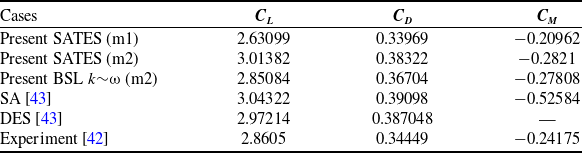
Comparison of aerodynamic coefficients of DLR-F11

Figure 13.

The contour of instantaneous flow and resolution control function.

Table 2 compares the aerodynamic coefficients, such as lift, drag and moment coefficient, along with the results of the experiment [Reference Rumsey and Slotnick42] and other numerical simulations [Reference Escobar, Suarez, Silva, López, Velandia and Lara43]. The lift coefficient of the present numerical simulation results is slightly higher than experimental data, which is also found in the previous simulaiton study [Reference Escobar, Suarez, Silva, López, Velandia and Lara43]. The drag coefficient and moment coefficient are generally in good agreement with the measurements. The results indicates that the current numerical results may tend a slightly delayed stall angle-of-attack, which is similar to the DES and SA turbulence models reported in the previous literature [Reference Escobar, Suarez, Silva, López, Velandia and Lara43].

The swept, medium/high-aspect-ratio wings of DLR-F11 configuration promotes three-dimensional flows around the wings, leading to the significant changes of the pressure coefficient C _p distributions along the spanwise direction. Figure 14 shows the comparison of the predicted pressure coefficient distributions and experimental data at the four different spanwise locations (η = 28.8%, 54.3%, 75.1%, 89.1%). It can be seen that the present SATES results based on finer grid-m2 are generally in good agreement with results of BSL k∼ω and the experimental data. Meanwhile, the maximum deviation exists on the wing tip of the flap at η = 89.1%, which indicates that the predicted results is approaching the stall condition.

Figure 14.

The distributions of pressure coefficient on the wing of DLR-F11.