1 Introduction
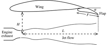
Aircraft noise is believed to be one of the most commonly reported residential disturbances (Pepper, Nascarella & Kendall Reference Pepper, Nascarella and Kendall2003). Among the different noise sources, jet noise is found to be the dominant component at takeoff. For the past few decades, jet noise has been one of the most heavily investigated subjects and the outcome has been quite successful. However, it is worth noting that the vast majority of research work during this time is for an isolated nozzle and jet. But the realistic configuration of a modern aircraft often involves the jet engines installed below the aircraft wings, as shown in figure 1. The effects of wings and other high-lift devices on the jet noise are often referred to as jet installation effects, and the resulting jet is commonly called an installed jet and compared to the isolated jet. Research has shown that the presence of solid boundaries can greatly affect acoustic source behaviours (Curle Reference Curle1955; Williams & Hall Reference Williams and Hall1970). Consequently, the close presence of aircraft wings can significantly alter the jet noise heard in the far-field (Bushell Reference Bushell1975; Fisher, Harper-Bourne & Glegg Reference Fisher, Harper-Bourne and Glegg1977; Way & Turner Reference Way and Turner1980; Shearin Reference Shearin1983). Investigation into the installed jet noise has been, however, rather limited. In particular, there is a general lack of reliable prediction models and also of understanding of the noise modification mechanism. This paper aims to contribute to bridging that gap: to develop a reliable model that can predict the installed jet noise and to advance the understanding of the noise amplification mechanism.
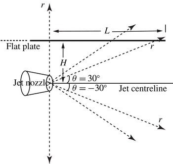
The schematic illustration of an installed engine. The distance between the jet centreline and the under surface of the wing is denoted by
 $H$
while the axial distance between the nozzle exit and the trailing edge of the flap is denoted by
 $L$
.

For the configuration shown in figure 1, there are two important geometric parameters defining the position of the engine relative to the wing: the distance
 $H$
between the jet centreline and the wing surface, and the distance
 $L$
between jet nozzle and the trailing edge of the flap. As far as the installed jet noise is concerned, one expects the jet operating condition to have an important impact on the sound radiated to the far-field, as described by the jet nozzle diameter
 $D$
, the jet exit velocity
 $V$
, the jet spread rate
 $\unicode[STIX]{x1D6FD}$
and the temperature ratio
 $T_{r}$
in the case of hot jets. In this paper, the impact of varying
 $H$
and
 $L$
on the far-field noise will be referred to as the engine position effect, while that of varying
 $D$
,
 $V$
and
 $\unicode[STIX]{x1D6FD}$
will be called the jet condition effect. When the flap is deployed, the flap length
 $F$
, the deflected angle
 $\unicode[STIX]{x1D6FC}$
and the width
 $W$
of flap cut-out in a real flight vehicle have influences on the installed jet noise, and this is similarly given the name the flap position effect.
The extra noise produced by an installed engine was first noticed by Bushell (Reference Bushell1975), who compared the in-flight installed jet noise with the static isolated jet noise for a full-scale aircraft. Many investigations followed, and they fall roughly into three categories: identifying installed noise sources by studying the acoustic characteristics of an installed jet, the engine position, jet condition and flap position effects; developing installed jet noise prediction models; and investigating noise reduction techniques. The first category includes the experimental work of Head & Fisher (Reference Head and Fisher1976), Szewczyk (Reference Szewczyk1979), Way & Turner (Reference Way and Turner1980), Shearin (Reference Shearin1983), Mead & Strange (Reference Mead and Strange1998) and Brown (Reference Brown2013). Through their experimental work, it was found that increasing
 $H$
results in less noise at low frequencies, while decreasing
 $L$
follows the same trend and raises the frequency of maximum augmentation due to installation effects. The velocity dependence of the peak of this low-frequency augmentation is to the fifth to sixth power. It was also confirmed that the low-frequency noise enhancement has a dipole-like directivity pattern. The numerical work carried out by Bondarenko, Hu & Zhang (Reference Bondarenko, Hu and Zhang2012) also falls into the first category, and sheds more light on the understanding of installed jet noise via flow field visualization.
In conjunction with the above experimental and numerical studies of installed jet noise characteristics, attempts to develop prediction models for installed jet noise have also been made. These include the work by Sengupta (Reference Sengupta1983), Stevens, Bryce & Szewczyk (Reference Stevens, Bryce and Szewczyk1983), Bhat & Blackner (Reference Bhat and Blackner1998) and Moore (Reference Moore2004). With the exception of Moore’s model, which is based on three-dimensional ray theory and jet blockage profiles, and gives encouraging results at high frequencies, the prediction models proposed at this time were generally empirical, i.e. by fitting experimental data or superimposing parametric changes heuristically. Thus, these models were inherently unable to capture detailed characteristics of installed jet noise correctly or to enhance physical understanding of the mechanisms. However, very recently some less-empirical models were proposed, including the work of Vera, Self & Kingan (Reference Vera, Self and Kingan2015) and Piantanida et al. (Reference Piantanida, Jaunet, Huber, Wolf, Jordan and Cavalieri2015). In Vera’s work, for an assumed plane-wave-like incident field, the scattered pressure on the surface of a semi-infinite flat plate is obtained by making use of the Wiener–Hopf method and the far-field sound is obtained using Amiet’s approach. However, the proposed form of the statistical spectrum of ‘the incident field required to calculate the far-field sound is hard to obtain in experimental measurements’. In addition, the ambient flow (non-trivial in a real flight certification process) is neglected in their modelling. Piantanida et al. (Reference Piantanida, Jaunet, Huber, Wolf, Jordan and Cavalieri2015) adopted another approach in their work, where the half-plane scattering Green’s function and an inferred near-field pressure source of the wave-packet form were used. The far-field sound is obtained by performing numerical integration. Both experimental measurements and numerical model predictions for low-frequency installed jet noise were presented, and ‘a good overall agreement with the experiments in terms of the dependence of the radiated levels and directivity on the radial jet-plate separation and sweep angle’ is achieved. In Piantanida’s work, a boundary element method (BEM) calculation is also performed as a validation for the Green’s function approach. The same technique was used earlier by Papamoschou (Reference Papamoschou2010) to predict the jet noise shielding effects with an inferred wavepackage and a monopole as sources. Reasonable results were obtained, with limitations at high frequencies caused by the deterministic characteristics of the sound sources. Attempts trying to reduce the installation effects of jet noise, as characterized by the third category, were first made by Wang (Reference Wang1981). In his paper, Wang reported an experimental test of jet noise performed on wing models made of materials with different acoustic surface properties. The experimental results showed that wing models with specially treated surfaces can substantially reduce the noise enhancement at high frequencies. Of practical interest, it was mentioned by Piantanida et al. (Reference Piantanida, Jaunet, Huber, Wolf, Jordan and Cavalieri2015) that, if the wing is swept, the installed jet noise can be reduced effectively, and the larger the swept angle is, the more the sound is reduced.
Hitherto, there has been little doubt about the mechanism of installation effects on noise at high frequencies: the noise is generated by small-scale eddies in the jet and reflected off the wing and flap surface; the reflected noise is refracted and attenuated by the presence of the turbulent jet plume. On the other hand, the noise mechanism at low frequencies has not been accepted unanimously. One of the proposed ideas was that the noise is due to the trailing-edge scattering, while Shearin (Reference Shearin1983) suggested a jet–surface interaction mechanism and Pastouchenko & Tam (Reference Pastouchenko and Tam2007) argued that it is the downwash effect of the wing flap causing more turbulence in the jet that is the principal mechanism. However, examination of the acoustic properties of the low-frequency installed noise and its dependence on the engine position, jet condition and flap position leads one to believe that the dominant effect is the trailing-edge noise. This is because the dipole characteristics are in agreement with the observed directivity pattern of trailing-edge noise at low frequencies (Amiet Reference Amiet1976b
; Head & Fisher Reference Head and Fisher1976; Wang Reference Wang1981; Mead & Strange Reference Mead and Strange1998; Roger & Moreau Reference Roger and Moreau2005; Bondarenko et al.
Reference Bondarenko, Hu and Zhang2012; Brown Reference Brown2013), decreasing
 $L$
results in a reduced noise and a frequency shift towards high frequencies (Head & Fisher Reference Head and Fisher1976; Way & Turner Reference Way and Turner1980; Wang Reference Wang1981; Shearin Reference Shearin1983; Stevens et al.
Reference Stevens, Bryce and Szewczyk1983), there exists a high correlation between the pressure field near the trailing edge and the far-field sound (Head & Fisher Reference Head and Fisher1976) and the dependence of sound intensity on the characteristic jet velocity is to the fifth to sixth power (Head & Fisher Reference Head and Fisher1976; Brown Reference Brown2013). These trailing-edge noise characteristics remind us of the suitability of Amiet’s approach in modelling low-frequency installed jet noise.
Section 2 presents the detailed derivation of our hybrid model. Section 3 then presents results based on the new model, and comparison with experimental data is also shown. Section 4 gives a brief conclusion of this paper.
2 Model formulation
Acoustic analogy theories have long been the standard approaches to predict jet noise, and they have proved to be sufficient in predicting isolated jet noise (Lighthill Reference Lighthill1952; Williams Reference Williams1963; Lilley Reference Lilley1974; Goldstein Reference Goldstein2003). We attempt to adopt the same approaches to the modelling of installed jet noise. However, as we will see in subsequent sections, conventional acoustic analogy theories fail to capture an additional but important noise generation mechanism. Consequently, in this section we use Lighthill’s acoustic analogy theory in conjunction with an additional near-field scattering theory to predict the far-field sound of installed cold jets at low Mach numbers, which naturally divides this section into two parts.
2.1 Lighthill’s acoustic analogy
In Lighthill’s original work (Lighthill Reference Lighthill1952, Reference Lighthill1954), turbulence-generated noise was studied in the absence of any solid boundaries. The effect of boundaries on sound generation aerodynamically was investigated by Curle (Reference Curle1955). Curle’s theory states that the effect of a solid boundary is equivalent to a distribution of dipole sources (unsteady force source) in addition to Lighthill’s quadrupole sources. The dipole strength is equal to the surface pressure. Therefore, in order to use Curle’s approach to calculate far-field sound, the pressure on the solid boundaries has to be known beforehand. The pressure on the surface of the plate depends on the quadrupole sources, and is difficult to obtain when the surface is non-compact, where there may be significant phase cancellation of the sound from the dipole sources. An alternative approach, which is much more advantageous, is that one can use the Green’s function that satisfies the boundary conditions on the solid surfaces. Then, the far-field sound, including both the incident field due to the quadrupole sources and the scattered field due to solid boundaries, can be readily obtained by performing a volume integration of the product of the Green’s function and the quadrupole sources. This is the approach that we use in this paper.
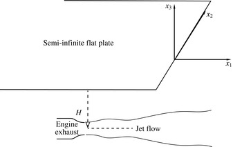
Schematic of the simplified model with a semi-infinite flat plate.

To use the latter approach, the Green’s function satisfying the rigid-wall boundary conditions at the upper and lower surfaces of the aircraft wing and flap needs to be obtained. While this could be done numerically by, for example, the boundary element method, we seek an analytical solution so that the physics of the jet–wing interaction can be understood. Therefore, we simplify the geometry by replacing the wing–flap system with a semi-infinite flat plate, as shown in figure 2. This is believed to be valid especially when the acoustic wavelength is shorter than the wing size (Amiet Reference Amiet1976b ; Roger & Moreau Reference Roger and Moreau2005). Then we start with the equation obtained by Lighthill (Lighthill Reference Lighthill1952), i.e.
 $$\begin{eqnarray}\left(\frac{\unicode[STIX]{x2202}^{2}}{\unicode[STIX]{x2202}t^{2}}-c_{0}^{2}\unicode[STIX]{x1D6FB}^{2}\right)(\unicode[STIX]{x1D70C}-\unicode[STIX]{x1D70C}_{0})=\frac{\unicode[STIX]{x2202}^{2}T_{ij}}{\unicode[STIX]{x2202}x_{i}\unicode[STIX]{x2202}x_{j}},\end{eqnarray}$$
where
 $x_{i}\,(i=1,2,3)$
denote the Cartesian coordinates shown in figure 2,
 $\unicode[STIX]{x1D70C}$
the fluid density,
 $\unicode[STIX]{x1D70C}_{0}$
the ambient fluid density,
 $c_{0}$
the speed of sound in the ambient fluid, and Lighthill’s stress tensor has the form of
 $$\begin{eqnarray}T_{ij}=\unicode[STIX]{x1D70C}u_{i}u_{j}+p_{ij}-(\unicode[STIX]{x1D70C}-\unicode[STIX]{x1D70C}_{0})c_{0}^{2}\unicode[STIX]{x1D6FF}_{ij},\end{eqnarray}$$
where
 $u_{i}$
and
 $u_{j}$
are the velocity components in the
 $i$
and
 $j$
direction, respectively, and
 $p_{ij}$
is the stress tensor. When the Reynolds number is high, which is so for most industrially relevant jet flows (and for many laboratory jets), the viscous terms in
 $T_{ij}$
can be ignored (Lighthill Reference Lighthill1952; Goldstein Reference Goldstein2003; Karabasov et al.
Reference Karabasov, Afsar, Hynes, Dowling, McMullan, Pokora, Page and McGuirk2010). Also when the mean temperature of the jet is the same as that of the ambient fluid, which is a good approximation for cold jets at low Mach numbers, the assumption that fluctuations in pressure are balanced out by the product of the density fluctuations and
 $c_{0}^{2}$
can be made (Lighthill Reference Lighthill1952).
 $T_{ij}$
can thus be approximated by
 $$\begin{eqnarray}T_{ij}\approx \unicode[STIX]{x1D70C}u_{i}u_{j}.\end{eqnarray}$$
In realistic full-scale tests, there exists a uniform ambient flow
 $U$
in the
 $x_{1}$
direction due to the forward flight of the aircraft. We aim to include this ambient mean-flow effect in our model, and to do that it is convenient to express the fluid velocity in terms of the fluctuation velocity (relative to the background flow)
 $u_{j}^{b}$
, i.e.
 $u_{i}=u_{i}^{b}+U\unicode[STIX]{x1D6FF}_{i1}$
. Substituting this definition into (2.1), and making use of the mass conservation equation, (2.1) can be formulated as
 $$\begin{eqnarray}\left(\frac{\unicode[STIX]{x2202}}{\unicode[STIX]{x2202}t}+U\frac{\unicode[STIX]{x2202}}{\unicode[STIX]{x2202}x_{1}}\right)^{2}\unicode[STIX]{x1D70C}^{\prime }-c_{0}^{2}\unicode[STIX]{x1D6FB}^{2}\unicode[STIX]{x1D70C}^{\prime }=\frac{\unicode[STIX]{x2202}^{2}\unicode[STIX]{x1D70C}u_{i}^{b}u_{j}^{b}}{\unicode[STIX]{x2202}x_{i}\unicode[STIX]{x2202}x_{j}},\end{eqnarray}$$
where we define the density fluctuation
 $\unicode[STIX]{x1D70C}^{\prime }\equiv \unicode[STIX]{x1D70C}-\unicode[STIX]{x1D70C}_{0}$
. By assuming an
 $\text{e}^{\text{i}\unicode[STIX]{x1D714}t}$
time dependence, (2.4) can be written as
 $$\begin{eqnarray}\left(\text{i}\unicode[STIX]{x1D714}+U\frac{\unicode[STIX]{x2202}}{\unicode[STIX]{x2202}x_{1}}\right)^{2}\unicode[STIX]{x1D70C}^{\prime }(\boldsymbol{x},\unicode[STIX]{x1D714})-c_{0}^{2}\unicode[STIX]{x1D6FB}^{2}\unicode[STIX]{x1D70C}^{\prime }(\boldsymbol{x},\unicode[STIX]{x1D714})=\frac{\unicode[STIX]{x2202}^{2}\hat{T}_{ij}(\boldsymbol{x},\unicode[STIX]{x1D714})}{\unicode[STIX]{x2202}x_{i}\unicode[STIX]{x2202}x_{j}},\end{eqnarray}$$
where
 $\unicode[STIX]{x1D70C}^{\prime }(\boldsymbol{x},\unicode[STIX]{x1D714})$
and
 $\hat{T}_{ij}(\boldsymbol{y},\unicode[STIX]{x1D714})$
are the Fourier transformations of
 $\unicode[STIX]{x1D70C}^{\prime }(\boldsymbol{x},t)$
and
 $\unicode[STIX]{x1D70C}u_{i}^{b}u_{j}^{b}$
, respectively.
Note that although we subtract the ambient uniform flow
 $U$
from
 $u_{i}$
, the source term on the right-hand side of (2.5) still comprises of both linear and nonlinear fluctuation terms. The linear terms are known to account for the jet mean-flow refraction effects, and should be most appropriately treated as a propagation effects rather than sources (Lighthill Reference Lighthill1952; Lilley Reference Lilley1974; Goldstein Reference Goldstein2003). We do not take the jet mean-flow propagation effects into account. Hence, when modelling the sources on the right-hand side of (2.5), only the nonlinear fluctuation terms (the Favre average is used for velocities, see Goldstein (Reference Goldstein2003) for example) are used. However, one can expect this to be acceptable both at low frequencies and for an observer at
 $90^{\circ }$
to the jet centreline, where the refraction effects are negligible. Now, provided the source terms are known, (2.5) can be solved by making use of the Green’s function satisfying appropriate boundary conditions. In the following sections, the Green’s function is developed first, then the source term is obtained by performing computational fluid dynamics (CFD) calculations.
2.1.1 The acoustic Green’s function
From (2.5), the Green’s function satisfies the convective wave equation
 $$\begin{eqnarray}\left(\text{i}\unicode[STIX]{x1D714}+U\frac{\unicode[STIX]{x2202}}{\unicode[STIX]{x2202}x_{1}}\right)^{2}G(\boldsymbol{x};\,\boldsymbol{y})-c_{0}^{2}\unicode[STIX]{x1D6FB}^{2}G(\boldsymbol{x};\,\boldsymbol{y})=\unicode[STIX]{x1D6FF}(\boldsymbol{x}-\boldsymbol{y}).\end{eqnarray}$$
This equation, together the rigid-wall boundary conditions at the upper and lower surfaces of the flat plate, needs to be solved to obtain the Green’s function.
Letting
 $k=\unicode[STIX]{x1D714}/c_{0}$
,
 $M=U/c_{0}$
, and
 $\unicode[STIX]{x1D6FD}^{2}=1-M^{2}$
, and then making the coordinate transformation,
 $x_{1}=\bar{x}_{1}$
,
 $x_{2}=\bar{x}_{2}/\unicode[STIX]{x1D6FD}$
,
 $x_{3}=\bar{x}_{3}/\unicode[STIX]{x1D6FD}$
,
 $y_{1}=\bar{y}_{1}$
,
 $y_{2}=\bar{y}_{2}/\unicode[STIX]{x1D6FD}$
and
 $y_{3}=\bar{y}_{3}/\unicode[STIX]{x1D6FD}$
, we can show that the solution to (2.6) (satisfying the rigid-wall boundary conditions on the upper and lower surfaces of the semi-infinite plate) can be found (Macdonald Reference Macdonald1915; Lyu & Dowling Reference Lyu and Dowling2016) as
 $$\begin{eqnarray}G_{f}=\frac{\unicode[STIX]{x1D6FD}^{2}\,\text{e}^{-\text{i}(kM/\unicode[STIX]{x1D6FD}^{2})\bar{y}_{1}}}{4\unicode[STIX]{x03C0}c_{0}^{2}}\left(\frac{\text{e}^{-\text{i}(k/\unicode[STIX]{x1D6FD}^{2})R}}{R}E(u_{R})+\frac{\text{e}^{-\text{i}(k/\unicode[STIX]{x1D6FD}^{2})R^{\prime }}}{R^{\prime }}E(u_{R^{\prime }})\right)\!,\end{eqnarray}$$
where
 $E(x)$
is an error function defined by
 $$\begin{eqnarray}E(x)=\frac{\text{e}^{\text{i}\unicode[STIX]{x03C0}/4}}{\sqrt{\unicode[STIX]{x03C0}}}\int _{-\infty }^{x}\,\text{e}^{-\text{i}u^{2}}\,\text{d}u,\end{eqnarray}$$
and
 $R$
and
 $R^{\prime }$
are given by
 $$\begin{eqnarray}\left.\begin{array}{@{}c@{}}\displaystyle R=\sqrt{(x_{1}-y_{1})^{2}+\unicode[STIX]{x1D6FD}^{2}(x_{2}-y_{2})^{2}+\unicode[STIX]{x1D6FD}^{2}(x_{3}-y_{3})^{2}},\\ \displaystyle R^{\prime }=\sqrt{(x_{1}+y_{1})^{2}+\unicode[STIX]{x1D6FD}^{2}(x_{2}+y_{2})^{2}+\unicode[STIX]{x1D6FD}^{2}(x_{3}+y_{3})^{2}}.\end{array}\right\}\end{eqnarray}$$
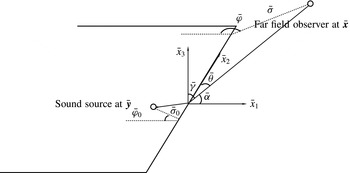
The schematic illustration of the stretched coordinates.

Here
 $$\begin{eqnarray}\left.\begin{array}{@{}c@{}}\displaystyle u_{R}=2\sqrt{{\displaystyle \frac{k\bar{\unicode[STIX]{x1D70E}}\bar{\unicode[STIX]{x1D70E}}_{0}}{\unicode[STIX]{x1D6FD}^{2}(S+R)}}}\cos \left(\frac{\bar{\unicode[STIX]{x1D711}}-\bar{\unicode[STIX]{x1D711}}_{0}}{2}\right),\\ \displaystyle u_{R^{\prime }}=2\sqrt{{\displaystyle \frac{k\bar{\unicode[STIX]{x1D70E}}\bar{\unicode[STIX]{x1D70E}}_{0}}{\unicode[STIX]{x1D6FD}^{2}(S+R^{\prime })}}}\cos \left(\frac{\bar{\unicode[STIX]{x1D711}}+\bar{\unicode[STIX]{x1D711}}_{0}}{2}\right),\end{array}\right\}\end{eqnarray}$$
where
 $S=\sqrt{(\bar{\unicode[STIX]{x1D70E}}+\bar{\unicode[STIX]{x1D70E}}_{0})^{2}+(\bar{z}-\bar{z}_{0})^{2}}$
and
 $(\bar{\unicode[STIX]{x1D70E}},\,\bar{\unicode[STIX]{x1D711}},\,\bar{z})$
and
 $(\bar{\unicode[STIX]{x1D70E}}_{0},\,\bar{\unicode[STIX]{x1D711}}_{0},\,\bar{z}_{0})$
denote the corresponding cylindrical coordinates of the observer location and sound source location in the stretched Cartesian coordinate system
 $(\bar{x}_{1},\,\bar{x}_{2},\,\bar{x}_{3})$
, respectively, as shown in figure 3. It is straightforward to show that
 $$\begin{eqnarray}\left.\begin{array}{@{}c@{}}\displaystyle \bar{\unicode[STIX]{x1D70E}}=\sqrt{x_{1}^{2}+\unicode[STIX]{x1D6FD}^{2}x_{3}^{2}},\quad \bar{\unicode[STIX]{x1D70E}}_{0}=\sqrt{y_{1}^{2}+\unicode[STIX]{x1D6FD}^{2}y_{3}^{2}},\\ \displaystyle \cos (\bar{\unicode[STIX]{x1D711}})=\frac{-x_{1}}{\bar{\unicode[STIX]{x1D70E}}},\quad \cos (\bar{\unicode[STIX]{x1D711}}_{0})=\frac{-y_{1}}{\bar{\unicode[STIX]{x1D70E}}_{0}},\\ \displaystyle \bar{z}=\unicode[STIX]{x1D6FD}x_{2},\quad \bar{z}_{0}=\unicode[STIX]{x1D6FD}y_{2}.\end{array}\right\}\end{eqnarray}$$
Similarly, the corresponding spherical coordinates of the observer and source positions in the stretched coordinate system are represented by
 $(\bar{r},\,\bar{\unicode[STIX]{x1D703}},\,\bar{\unicode[STIX]{x1D711}})$
and
 $(\bar{r}_{0},\,\bar{\unicode[STIX]{x1D703}}_{0},\,\bar{\unicode[STIX]{x1D711}}_{0})$
, respectively.
When the far-field observer assumption is invoked, the second derivatives of the Green’s function can be obtained as
 $$\begin{eqnarray}\displaystyle & \displaystyle \frac{\unicode[STIX]{x2202}^{2}G(\boldsymbol{x};\,\boldsymbol{y})}{\unicode[STIX]{x2202}y_{2}^{2}}=A(\boldsymbol{x},y_{1},y_{2})k^{2}D_{22}^{0}(y_{1},y_{3}), & \displaystyle\end{eqnarray}$$
 $$\begin{eqnarray}\displaystyle & \displaystyle \frac{\unicode[STIX]{x2202}^{2}G(\boldsymbol{x};\,\boldsymbol{y})}{\unicode[STIX]{x2202}y_{1}\unicode[STIX]{x2202}y_{2}}=A(\boldsymbol{x},y_{1},y_{2})k^{2}\left(D_{12}^{0}(y_{1},y_{3})+\sqrt{\displaystyle {\displaystyle \frac{1}{k\bar{\unicode[STIX]{x1D70E}}_{0}}}}D_{12}^{1}(y_{1},y_{3})\right)\!, & \displaystyle\end{eqnarray}$$
 $$\begin{eqnarray}\displaystyle & \displaystyle \frac{\unicode[STIX]{x2202}^{2}G(\boldsymbol{x};\,\boldsymbol{y})}{\unicode[STIX]{x2202}y_{2}\unicode[STIX]{x2202}y_{3}}=A(\boldsymbol{x},y_{1},y_{2})k^{2}\left(D_{23}^{0}(y_{1},y_{3})+\sqrt{\displaystyle {\displaystyle \frac{1}{k\bar{\unicode[STIX]{x1D70E}}_{0}}}}D_{23}^{1}(y_{1},y_{3})\right)\!, & \displaystyle\end{eqnarray}$$
 $$\begin{eqnarray}\displaystyle \displaystyle \frac{\unicode[STIX]{x2202}^{2}G(\boldsymbol{x};\,\boldsymbol{y})}{\unicode[STIX]{x2202}y_{1}^{2}} & = & \displaystyle A(\boldsymbol{x},y_{1},y_{2})k^{2}\nonumber\\ \displaystyle & & \displaystyle \times \!\left(D_{11}^{0}(y_{1},y_{3})+\sqrt{\displaystyle {\displaystyle \frac{1}{k\bar{\unicode[STIX]{x1D70E}}_{0}}}}D_{11}^{1}(y_{1},y_{3})+\left(\sqrt{\displaystyle {\displaystyle \frac{1}{k\bar{\unicode[STIX]{x1D70E}}_{0}}}}\right)^{3}D_{11}^{2}(y_{1},y_{3})\right)\!,\nonumber\\ \displaystyle & & \displaystyle\end{eqnarray}$$
 $$\begin{eqnarray}\displaystyle \displaystyle \frac{\unicode[STIX]{x2202}^{2}G(\boldsymbol{x};\,\boldsymbol{y})}{\unicode[STIX]{x2202}y_{3}^{2}} & = & \displaystyle A(\boldsymbol{x},y_{1},y_{2})k^{2}\nonumber\\ \displaystyle & & \displaystyle \times \!\left(D_{33}^{0}(y_{1},y_{3})+\sqrt{\displaystyle {\displaystyle \frac{1}{k\bar{\unicode[STIX]{x1D70E}}_{0}}}}D_{33}^{1}(y_{1},y_{3})+\left(\sqrt{\displaystyle {\displaystyle \frac{1}{k\bar{\unicode[STIX]{x1D70E}}_{0}}}}\right)^{3}D_{33}^{2}(y_{1},y_{3})\right)\!,\nonumber\\ \displaystyle & & \displaystyle\end{eqnarray}$$
 $$\begin{eqnarray}\displaystyle \displaystyle \frac{\unicode[STIX]{x2202}^{2}G(\boldsymbol{x};\,\boldsymbol{y})}{\unicode[STIX]{x2202}y_{1}\unicode[STIX]{x2202}y_{3}} & = & \displaystyle A(\boldsymbol{x},y_{1},y_{2})k^{2}\nonumber\\ \displaystyle & & \displaystyle \times \!\left(D_{13}^{0}(y_{1},y_{3})+\sqrt{\displaystyle {\displaystyle \frac{1}{k\bar{\unicode[STIX]{x1D70E}}_{0}}}}D_{13}^{1}(y_{1},y_{3})+\left(\sqrt{\displaystyle {\displaystyle \frac{1}{k\bar{\unicode[STIX]{x1D70E}}_{0}}}}\right)^{3}D_{13}^{2}(y_{1},y_{3})\right)\!,\nonumber\\ \displaystyle & & \displaystyle\end{eqnarray}$$
where
 $$\begin{eqnarray}A(\boldsymbol{x},y_{1},y_{2})=\frac{\unicode[STIX]{x1D6FD}^{2}\,\text{e}^{-\text{i}(k/\unicode[STIX]{x1D6FD}^{2})\bar{r}}\,\text{e}^{\text{i}(kM/\unicode[STIX]{x1D6FD}^{2})x_{1}}}{4\unicode[STIX]{x03C0}c_{0}^{2}\bar{r}}\,\text{e}^{\text{i}(k/\unicode[STIX]{x1D6FD}^{2})\left(-M+\cos \bar{\unicode[STIX]{x1D6FC}}\right)y_{1}}\,\text{e}^{\text{i}(k/\unicode[STIX]{x1D6FD})\cos \bar{\unicode[STIX]{x1D703}}y_{2}},\end{eqnarray}$$
and the detailed expressions for
 $D_{ij}^{k}$
are shown in appendix A. The terms
 $D_{ij}^{k}$
are properly bounded functions and determine the directivity patterns of the radiation from the corresponding quadrupoles. Therefore, the noise enhancement arises from the terms
 $\sqrt{1/(k\bar{\unicode[STIX]{x1D70E}}_{0})}$
and
 $\sqrt{1/(k\bar{\unicode[STIX]{x1D70E}}_{0})^{3}}$
appearing in front of
 $D_{ij}^{1}$
and
 $D_{ij}^{2}$
, respectively. When the frequency is sufficiently low, or the quadrupole source is sufficiently close to the edge of the flat plate, the far-field sound is dominated by the term involving
 $\sqrt{1/(k\bar{\unicode[STIX]{x1D70E}}_{0})}$
in the derivatives normal to the 2-axis, and is much larger than that when the plate is absent. The derivatives with one
 $y_{2}$
derivative have leading terms involving
 $\sqrt{1/(k\bar{\unicode[STIX]{x1D70E}}_{0})}$
, and therefore are not as efficient as those derivatives involving
 $\sqrt{1/(k\bar{\unicode[STIX]{x1D70E}}_{0})^{3}}$
at low frequencies. Equation (2.12), however, does not involve enhanced terms, hence quadrupoles aligned with the 2-axis (corresponding to
 $\unicode[STIX]{x2202}^{2}G(\boldsymbol{x};\,\boldsymbol{y})/\unicode[STIX]{x2202}y_{2}^{2}$
) are the least efficient sound sources when close to the edge.
2.1.2 CFD flow field calculation
We have obtained the Green’s function for the scattering problem in the preceding section. In order to solve (2.5) to determine the sound from the Lighthill quadrupoles, we need to obtain the source terms shown on the right-hand side of (2.5). Unsteady numerical simulations such as large eddy simulations (LES) are well suited for such a purpose. However, performing an LES study is computationally expensive. The usual time required even on a massively parallel computer can vary from a few days to many weeks, depending on practical needs. To avoid this difficulty, attempts to use time-averaged flow calculations to predict isolated jet noise have been made by many authors. For example, Khavaran, Krejsa & Kim (Reference Khavaran, Krejsa and Kim1994), Bailly, Lafon & Candel (Reference Bailly, Lafon and Candel1994) and Bailly, Candel & Lafon (Reference Bailly, Candel and Lafon1996) used time-averaged calculations with turbulence statistics obtained from a
 $k-\unicode[STIX]{x1D716}$
turbulence model for predicting supersonic jet noise. In the work of Béchara et al. (Reference Béchara, Lafon, Bailly and Candel1995), a Reynolds-averaged Navier–Stokes (RANS) calculation incorporating a
 $k-\unicode[STIX]{x1D716}$
model for turbulence to characterize the sound sources was used to predict the noise of both simple and coaxial jets. Later, Tam & Auriault (Reference Tam and Auriault1999) further explored this approach and successfully predicted jet noise at
 $90^{\circ }$
to the jet by proposing an empirical sound source model analogous to gas kinetic theory. Moreover, the three empirical constants in Tam’s work were obtained by fitting to the far-field noise. In contrast, the work by Karabasov et al. (Reference Karabasov, Afsar, Hynes, Dowling, McMullan, Pokora, Page and McGuirk2010) is based on Goldstein’s acoustic analogy theory (Goldstein Reference Goldstein2003), and the proportionality constants used in its source model are obtained from analysing LES data, which therefore contains little empiricism apart from that of the
 $k-\unicode[STIX]{x1D716}$
model for turbulence. The predicted noise at various observer angles to the jet are found to agree well with experiments. In this study we adopt the same approach in order to yield fast predictions. Therefore, in this section we perform a RANS study with the standard
 $k-\unicode[STIX]{x1D716}$
turbulence model, and the source terms are subsequently modelled by making use of the time-averaged flow variables from the RANS, as will be described in detail in the next section.
The commercial software ANSYS Fluent 16.0 is used to perform a RANS calculation of an isolated round jet with the same temperature as the ambient air. When the wing and flap are sufficiently away from the jet, it can be expected that little change of the flow field occurs. Thus, as a starting point we first calculate the flow field for an axisymmetric jet. The computational domain is
 $30D$
and
 $5D$
in the streamwise and radial directions, respectively, where
 $D$
is the jet nozzle diameter. Calculations using much larger computational domains have shown little difference from those using the domain described above. The current domain size is therefore used to yield both a fast convergence and sufficiently accurate results.
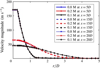
Velocity distributions in the radial direction using different meshes consisting of 0.8 million, 0.2 million and 0.1 million cells, respectively.

The mesh used in the calculation is generated using ANSYS Meshing 16.0. A structured quadrilateral mesh is used for the entire domain, and the mesh is much denser near the mixing layer and close to the jet. Near the mixing layer, the grid size is approximately
 $0.025D$
in the axial direction and
 $0.02D$
in the radial direction. The grid size inside the nozzle (
 $r<0.5D$
) in the radial direction is nearly uniformly
 $0.025D$
. Near the downstream boundary the grid size is approximately
 $0.2D$
. The mesh consists of approximately 0.1 million cells. To check the mesh independence, calculations using meshes consisting of 0.2 million and 0.8 million cells were carried out and the results yielded little difference, as shown in figure 4. It is shown that this number of cells (
 $0.1$
million) is sufficient to generate rapidly converging and sufficiently accurate results. A wall-function approach is used to resolve the boundary layer inside the nozzle. The chosen ‘standard wall function’ in ANSYS Fluent is based on the work of Launder and Spalding (Launder & Spalding Reference Launder and Spalding1974; ANSYS 2015). The boundary layer mesh starts at approximately
 $y^{+}=50$
, where
 $y^{+}$
is the dimensionless distance of the first mesh layer to the wall based on the wall friction velocity (White Reference White2005). The wall friction velocity
 $u^{\ast }$
is estimated using the log-law of the boundary layer (White Reference White2005). The boundary layer is resolved by approximately
 $15$
layers, which should be sufficient according to the Fluent Theory Guide (ANSYS 2015). Calculations using more layers show little difference for the mean and turbulent flow quantities.
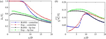
Comparison of the jet mean and root-mean-square axial fluctuation velocities along the centreline and lip line between the RANS and experimental data. Isotropic turbulence is assumed for the RANS to obtain the root-mean-square axial fluctuation velocity from turbulence intensity
 $k$
.

The boundary conditions for boundaries both upstream and downstream are ‘pressure outlets’ provided in ANSYS Fluent (ANSYS 2015). At the nozzle inlet boundary ‘pressure inlet’ is used (ANSYS 2015), which specifies both the stagnation pressure and the stagnation temperature. The stagnation pressure and stagnation temperature are given on the inlet boundary such that a Mach number
 $M_{0}=0.5$
jet is obtained, where
 $M_{0}=U_{j}/c_{0}$
, with
 $U_{j}$
being the mean jet exit velocity. The static temperature at the inlet boundary is the same as that of the ambient air, which is set to be
 $300$
K. The turbulence intensity at the ‘pressure inlet’ is set to be
 $5\,\%$
, and studies using other values have shown little change in the calculated flow field, especially after the potential core.
The standard
 $k-\unicode[STIX]{x1D716}$
model for the turbulence is used, as it gives a more realistic core length (see figure 5 for example) compared to other turbulent models such as the realizable
 $k-\unicode[STIX]{x1D716}$
model provided in ANSYS Fluent (ANSYS 2015). In fact, although the potential core length varies, the difference that changing turbulent models causes on the turbulent flow quantities is not significant, especially for the locations (
 $x>4D$
) where the sound generation is most efficient. Moreover, since the far-field sound depends on an integration over the whole turbulent flow field, little difference can be expected. As shown by Mohan et al. (Reference Mohan, Dowling, Karabasov, Xia, Graham, Hynes and Tucker2015), the use of many different turbulent models, such as
 $k-\unicode[STIX]{x1D716}$
,
 $k-\unicode[STIX]{x1D714}$
etc., makes little difference to the far-field sound spectrum over the entire frequency range. Therefore we think that the use of the
 $k-\unicode[STIX]{x1D716}$
model is sufficient for the current purpose. The compressible RANS equations are solved, and the ideal-gas law for air is adopted while the ambient pressure is set to be 1 atm. A model for the fourth-order space–time correlation function, as described in detail in the next section, can then be obtained from the flow variables
 $\bar{\unicode[STIX]{x1D70C}}$
,
 $\bar{\boldsymbol{u}}$
,
 $k$
and
 $\unicode[STIX]{x1D716}$
, which denote the mean density, mean velocities, turbulence intensity and turbulence dissipation rate, respectively.
To validate the RANS simulation, the streamwise components of the mean and fluctuation velocities (root-mean-square value), both along the lip line and centreline of jet, are compared with the experimental data published by Bridges (Bridges & Wernet Reference Bridges and Wernet2010), as shown in figure 5. The details of Bridges’ experiment will be discussed in § 2.2.1. From figure 5(a), it can be seen that the mean velocity profiles, in particular that on the lip line, agree well with experiment. On the centreline, the core length matches well with experimental data, though it appears that the velocity is slightly under-predicted further downstream. Given that the Reynolds number for Bridge’s experiment is twice that for the RANS simulation (as
 $D$
are
 $1$
in and
 $2$
in for the RANS and Bridge’s experiment, respectively) and the temperature ratio in the experiment is slightly different from that in the simulation, such agreement is good and the effect of any difference on the sound propagation can be expected to be negligible. Figure 5(b) shows the turbulent fluctuation velocity profiles on the jet lip line and centreline. The root-mean-square value of
 $u_{1}^{\prime }$
, where
 $u_{1}^{\prime }$
is the axial fluctuation velocity, is available in the experiment, but not from the RANS simulation. To facilitate comparison, we estimate this value from the turbulence intensity
 $k$
by assuming that the turbulence is isotropic. This assumption, however, is known not to be correct (Karabasov et al.
Reference Karabasov, Afsar, Hynes, Dowling, McMullan, Pokora, Page and McGuirk2010; Mohan et al.
Reference Mohan, Dowling, Karabasov, Xia, Graham, Hynes and Tucker2015); therefore, we expect a slight under-prediction of the axial turbulent fluctuation velocities, which can be seen from figure 5(b). Apart from these uncertainties, it can be seen that an overall good agreement is achieved for data on the lip line. The results on the centreline also agree well after approximately
 $x/D=6$
. The over-prediction in the first few diameters is expected. This is because the inlet turbulence intensity is given a high-than-normal value of
 $5\,\%$
, so that the centreline turbulence profiles near the downstream edge of the potential core can better agree with the experiment. However, as mentioned earlier, changing the inlet turbulence intensity has no effect on the flow field after the potential core.
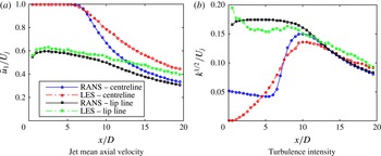
As will be mentioned in the rest of this paper, an LES study is also performed with the same operating conditions as those in Bridges’ experiment. Details of the LES can be found in § 2.2.1. It is therefore useful to compare the results of our RANS simulation to those obtained in the LES. Because we are now able to calculate the turbulence intensity directly from LES, we do not need to compare the root-mean-square of the axial fluctuation velocity by assuming isotropic turbulence for the RANS results. The results are shown in figure 6. It can be seen that a similar good agreement with that shown in figure 5(a) for the mean axial velocities is achieved. However, comparing figure 6(b) to figure 5(b), one sees a much better agreement for the turbulence intensity distribution, especially for the axial positions after the potential core. This shows that the cause of the under-prediction shown in figure 5(b) is indeed due to the assumption of isotropic turbulence (Karabasov et al. Reference Karabasov, Afsar, Hynes, Dowling, McMullan, Pokora, Page and McGuirk2010; Mohan et al. Reference Mohan, Dowling, Karabasov, Xia, Graham, Hynes and Tucker2015), and the RANS simulation is capable of predicting the jet flow accurately.
Comparison of the jet mean and turbulence intensity along the centreline and lip line between the RANS and LES results.

2.1.3 Far-field sound due to Lighthill’s quadrupoles
Combining the acoustic Green’s function, the model of the fourth-order space–time correlation function from Karabasov et al. (Reference Karabasov, Afsar, Hynes, Dowling, McMullan, Pokora, Page and McGuirk2010) and the mean-flow data from the RANS solution, we are now in a position to formulate the far-field sound power spectra. It is well established that the far-field sound perturbation can be written as
 $$\begin{eqnarray}\unicode[STIX]{x1D70C}^{\prime }(\boldsymbol{x},\unicode[STIX]{x1D714})=\int _{V}\hat{T}_{ij}(\boldsymbol{y},\unicode[STIX]{x1D714})\frac{\unicode[STIX]{x2202}^{2}G(\boldsymbol{x};\,\boldsymbol{y},\unicode[STIX]{x1D714})}{\unicode[STIX]{x2202}y_{i}\unicode[STIX]{x2202}y_{j}}\,\text{d}^{3}y.\end{eqnarray}$$
The integral in (2.19) is over the entire volume where
 $\hat{T}_{ij}(\boldsymbol{y},\unicode[STIX]{x1D714})$
is not second-order small. By making use of the linearized relationship
 $p^{\prime }(\boldsymbol{x},\unicode[STIX]{x1D714})=c_{0}^{2}\unicode[STIX]{x1D70C}^{\prime }(\boldsymbol{x},\unicode[STIX]{x1D714})$
and
 $\unicode[STIX]{x1D6F7}_{Q}(\boldsymbol{x},\unicode[STIX]{x1D714})=\lim _{T\rightarrow \infty }(\unicode[STIX]{x03C0}/T)\overline{p^{\prime }(\boldsymbol{x},\unicode[STIX]{x1D714})p^{\prime \ast }(\boldsymbol{x},\unicode[STIX]{x1D714})}$
, where
 $\unicode[STIX]{x1D6F7}_{Q}(\boldsymbol{x},\unicode[STIX]{x1D714})$
represents the power spectral density (PSD) of far-field sound and
 $\ast$
denotes taking the complex conjugate, it can be shown that
 $$\begin{eqnarray}\unicode[STIX]{x1D6F7}_{Q}(\boldsymbol{x},\unicode[STIX]{x1D714})=c_{0}^{4}\int _{V_{y}}\int _{V_{\unicode[STIX]{x0394}y}}R_{ijkl}(\boldsymbol{y},\unicode[STIX]{x0394}\boldsymbol{y},\unicode[STIX]{x1D714})I_{ijkl}(\boldsymbol{x},\boldsymbol{y},\unicode[STIX]{x0394}\boldsymbol{y},\unicode[STIX]{x1D714})\,\text{d}^{3}\unicode[STIX]{x0394}y\,\text{d}^{3}y,\end{eqnarray}$$
where
 $$\begin{eqnarray}\left.\begin{array}{@{}c@{}}\displaystyle R_{ijkl}(\boldsymbol{y},\unicode[STIX]{x0394}\boldsymbol{y},\unicode[STIX]{x1D714})=\frac{1}{2\unicode[STIX]{x03C0}}\int _{-\infty }^{\infty }\overline{T_{ij}(\boldsymbol{y},t)T_{kl}(\boldsymbol{y}+\unicode[STIX]{x0394}\boldsymbol{y},t+\unicode[STIX]{x1D70F})}\,\text{e}^{-\text{i}\unicode[STIX]{x1D714}\unicode[STIX]{x1D70F}}\,\text{d}\unicode[STIX]{x1D70F},\\ \displaystyle I_{ijkl}(\boldsymbol{x},\boldsymbol{y},\unicode[STIX]{x0394}\boldsymbol{y},\unicode[STIX]{x1D714})=\frac{\unicode[STIX]{x2202}^{2}G(\boldsymbol{x};\,\boldsymbol{y},\unicode[STIX]{x1D714})}{\unicode[STIX]{x2202}y_{i}\unicode[STIX]{x2202}y_{j}}\frac{\unicode[STIX]{x2202}^{2}G^{\ast }(\boldsymbol{x};\,\boldsymbol{y}+\unicode[STIX]{x0394}\boldsymbol{y},\unicode[STIX]{x1D714})}{\unicode[STIX]{x2202}y_{k}\unicode[STIX]{x2202}y_{l}}.\end{array}\right\}\end{eqnarray}$$
It is known that the fourth-order space–time correlation function
 $R_{ijkl}(\boldsymbol{y},\unicode[STIX]{x0394}\boldsymbol{y},\unicode[STIX]{x1D70F})$
can be well represented by a Gaussian function as (Karabasov et al.
Reference Karabasov, Afsar, Hynes, Dowling, McMullan, Pokora, Page and McGuirk2010)
 $$\begin{eqnarray}\displaystyle \hspace{-10.00002pt}R_{ijkl}(\boldsymbol{y},\unicode[STIX]{x0394}\boldsymbol{y},\unicode[STIX]{x1D70F}) & = & \displaystyle A_{ijkl}(\boldsymbol{y})\exp \left[-\frac{|\unicode[STIX]{x0394}y_{1}|}{\bar{u}_{1}(\boldsymbol{y})\unicode[STIX]{x1D70F}_{s}(\boldsymbol{y})}\right.\nonumber\\ \displaystyle & & \displaystyle \left.-\ln 2\left(\left(\frac{\unicode[STIX]{x0394}y_{1}-\bar{u}_{1}(\boldsymbol{y})\unicode[STIX]{x1D70F}}{l_{1}(\boldsymbol{y})}\right)^{2}+\left(\frac{\unicode[STIX]{x0394}y_{2}}{l_{2}(\boldsymbol{y})}\right)^{2}+\left(\frac{\unicode[STIX]{x0394}y_{3}}{l_{3}(\boldsymbol{y})}\right)^{2}\right)\right]\!,\end{eqnarray}$$
where
 $A_{ijkl}(\boldsymbol{y})=C_{ijkl}(2\bar{\unicode[STIX]{x1D70C}}k)^{2}$
,
 $l_{i}=c_{i}k^{3/2}/\unicode[STIX]{x1D716}$
and
 $\unicode[STIX]{x1D70F}_{s}=c_{\unicode[STIX]{x1D70F}}k/\unicode[STIX]{x1D716}$
. The constants
 $C_{ijkl}$
,
 $c_{i}$
and
 $c_{\unicode[STIX]{x1D70F}}$
can be obtained by best fitting (2.22) to the space–time correlation data obtained from LES simulations. By analysing the LES data, we found that
 $c_{1}$
,
 $c_{2}$
,
 $c_{3}$
,
 $c_{\unicode[STIX]{x1D70F}}$
are approximately
 $0.4$
,
 $0.23$
,
 $0.23$
,
 $0.3$
, respectively, which are close to those obtained by Karabasov et al. (Reference Karabasov, Afsar, Hynes, Dowling, McMullan, Pokora, Page and McGuirk2010), but also account for the anisotropy of the turbulence length scales (see Mohan et al.
Reference Mohan, Dowling, Karabasov, Xia, Graham, Hynes and Tucker2015).
 $C_{ijkl}$
remain the same as those found by Karabasov et al. (Reference Karabasov, Afsar, Hynes, Dowling, McMullan, Pokora, Page and McGuirk2010). The fourth-order space–time correlation of the nonlinear source term is known to be well modelled by (2.22) (see more details from Goldstein (Reference Goldstein2003) and Karabasov et al. (Reference Karabasov, Afsar, Hynes, Dowling, McMullan, Pokora, Page and McGuirk2010)). Using (2.22), the cross-spectra is thus obtained by performing the standard Fourier transformation, which yields
 $$\begin{eqnarray}\displaystyle R_{ijkl}(\boldsymbol{y},\unicode[STIX]{x0394}\boldsymbol{y},\unicode[STIX]{x1D714}) & = & \displaystyle \frac{l_{1}(\boldsymbol{y})}{2\bar{u}_{1}(\boldsymbol{y})\sqrt{\unicode[STIX]{x03C0}\ln 2}}A_{ijkl}(\boldsymbol{y})\exp \left[-\frac{l_{1}(\boldsymbol{y})^{2}\unicode[STIX]{x1D714}^{2}}{4\bar{u}_{1}^{2}(\boldsymbol{y})\ln 2}\right]\nonumber\\ \displaystyle & & \displaystyle \exp \left[-\frac{|\unicode[STIX]{x0394}y_{1}|}{\bar{u}_{1}(\boldsymbol{y})\unicode[STIX]{x1D70F}_{s}(\boldsymbol{y})}-\text{i}\frac{\unicode[STIX]{x1D714}}{\bar{u}_{1}(\boldsymbol{y})}\unicode[STIX]{x0394}y_{1}-\ln 2\left(\left(\frac{\unicode[STIX]{x0394}y_{2}}{l_{2}(\boldsymbol{y})}\right)^{2}+\left(\frac{\unicode[STIX]{x0394}y_{3}}{l_{3}(\boldsymbol{y})}\right)^{2}\right)\right]\!.\nonumber\\ \displaystyle & & \displaystyle\end{eqnarray}$$
The tensor
 $I_{ijkl}(\boldsymbol{x},\boldsymbol{y},\unicode[STIX]{x0394}\boldsymbol{y},\unicode[STIX]{x1D714})$
in (2.21) depends solely on the Green’s function. Consequently, substituting the free-space Green’s function or the one developed in the first part of this section into (2.20) yields results for an isolated jet or installed jet, respectively.
2.2 Near-field scattering
Outside the jet mixing layer, there is a region of near-field pressure fluctuations, which is primarily induced by hydrodynamic instability waves and decays exponentially in the radial direction (Jordan & Colonius Reference Jordan and Colonius2013). In the frequency regime
 $St>0.1$
, the waves convect at a virtually constant speed
 $U_{c}\approx 0.6\sim 0.8U_{j}$
, where
 $St$
is the Strouhal number based on the jet diameter (Arndt, Long & Glauser Reference Arndt, Long and Glauser1997; Tinney & Jordan Reference Tinney and Jordan2008; Gudmundsson & Colonius Reference Gudmundsson and Colonius2011; Jordan & Colonius Reference Jordan and Colonius2013). Since the convection velocity is lower than the speed of sound, the pressure due to the field of a hydrodynamic wave decays exponentially in the radial direction (see the details in the following section) and therefore only contributes weakly to the far-field of an isolated jet. When acoustic analogy theories are adopted for the isolated jet, these evanescent waves are not regarded as quadrupole sources, since their magnitude of fluctuation is small enough to be regarded as linear (pseudosound, thus their source strength would be second-order small). However, when a surface with sharp edges is present in the near-field of the jet, the previously non-radiating pressure field can be efficiently scattered into sound by the edge. Thus, this suggests that the Lighthill’s quadrupole sources are not sufficient to correctly predict the far-field of the installed jet, and the sound scattered by the sharp edges of the aerofoil must be accounted for. In this section, the far-field sound due to the interaction between the near-field evanescent waves and the plate edge is modelled using Amiet’s approach.
It is worth noting that the trailing-edge scattering mechanism of the hydrodynamic field has been suggested in several earlier works – for example, those of Lawrence, Azarpeyvand & Self (Reference Lawrence, Azarpeyvand and Self2011) and Bychkov & Faranosov (Reference Bychkov and Faranosov2014). However, the use of the term ‘hydrodynamic field’ is not always same as the evanescent wave mentioned here, for both nonlinear and linear regions of hydrodynamic field exist. The evanescent wave mentioned here accounts for only the exponentially decaying linear part (excluding both the nonlinear and linear acoustic parts), the mechanisms of which cannot be captured by Lighthill’s acoustic analogy. It should also be noted that the most heavily researched and cited convection velocity, which is approximately
 $0.6\sim 0.8U_{j}$
, is primarily for the instability waves at frequencies around
 $St=0.3$
. But whether this convection speed is still constant at very low frequencies is not yet known. In fact the constant-convection-velocity assumption has been called into question by several authors (Kerhervé, Fitzpatick & Jordan Reference Kerhervé, Fitzpatick and Jordan2006). By analysing LES data we confirmed the frequency dependence of the convection velocity and found that this convection velocity
 $U_{c}$
is significantly lower than
 $0.6U_{j}$
at low frequencies, e.g. for
 $St<0.1$
. This frequency dependence is included in our model.
2.2.1 The near-field evanescent waves
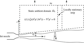
As the near-field evanescent waves are scattered into sound nearby the trailing edge, it is useful to investigate its properties before we move on to model the scattering mechanism, in particular its spatial correlation. To illustrate the idea, we consider here an isolated jet with static ambient flow, as shown in figure 7. Note that we work with an isolated jet in this section, thus it is sensible to temporarily switch to a cylindrical coordinate system with its origin located at the centre of the nozzle exit, as shown in figure 7. The axial and radial coordinates are denoted by
 $x$
and
 $r$
respectively. At any axial position
 $x$
, the mean jet velocity decays quickly (outside the potential core) as
 $r$
increases. Therefore, the velocity effectively vanishes when the radial distance from the jet centreline is larger than a value
 $r_{0}$
. Due to the spreading effect of the jet and the self-similarity exhibited by the velocity distribution along the radial lines,
 $r_{0}$
would increase as
 $x$
increases. Consequently, the pressure fluctuation when
 $r>r_{0}$
, as shown by the domain
 $\unicode[STIX]{x1D6FA}_{0}$
in figure 7, is governed by the classical wave equation resulting from the linearization of the perturbed Navier–Stokes equations, which is standard and not repeated here.
Schematic of the jet with a static ambient flow.
 $r$
,
 $\unicode[STIX]{x1D703}$
and
 $x$
denote the radial, azimuthal and streamwise coordinates, respectively. Immediately outside the jet plume where the flow velocity virtually vanishes, the linearized Navier–Stokes equation resulted in the classical wave equation. Due to the spreading of the jet flow, only the pressure fluctuation in the narrow strip might be regarded as a stationary function of
 $x$
.

The solution of the reduced wave equation for frequency
 $\unicode[STIX]{x1D714}$
in
 $\unicode[STIX]{x1D6FA}_{0}$
is also standard. If we are only interested the radially decaying components (excluding the oscillating acoustic components), the solution must be of the form
 $$\begin{eqnarray}p^{\prime }(\unicode[STIX]{x1D714},\boldsymbol{x})=\mathop{\sum }_{m=-\infty }^{\infty }\int _{-\infty }^{\infty }\hat{p}(\unicode[STIX]{x1D714},m,k_{x})K_{m}\left(\sqrt{k_{x}^{2}-k^{2}}r\right)\,\text{e}^{\text{i}m\unicode[STIX]{x1D703}}\,\text{e}^{-\text{i}k_{x}x}\,\text{d}k_{x},\end{eqnarray}$$
where
 $\unicode[STIX]{x1D703}$
is the azimuthal angle,
 $K_{m}(r)$
is the
 $m$
th modified Bessel function of the second kind, and we have made the use of the fact that the exponentially growing solution
 $I_{m}(r)$
tending to infinity as
 $r\rightarrow \infty$
must be excluded. As we have excluded the solutions corresponding to acoustic fluctuations, the integral interval of
 $k_{x}$
should strictly be from
 $-\infty$
to
 $-k$
and from
 $k$
to
 $\infty$
. However, since this does not affect our following derivation, we will use the interval from
 $-\infty$
to
 $\infty$
for simplicity.
Since the flow field is turbulent in time
 $t$
,
 $\hat{p}(\unicode[STIX]{x1D714},m,k_{x})$
would be a statistical quantity with respect to
 $\unicode[STIX]{x1D714}$
. In addition, the turbulence flow also results in randomness of the boundary condition of the domain
 $\unicode[STIX]{x1D6FA}_{0}$
, so it can be expected that
 $\hat{p}(\unicode[STIX]{x1D714},m,k_{x})$
would be a statistical quantity with respect to
 $m$
and
 $k_{x}$
as well. Therefore, the cross power spectral density of two points located at the same
 $x$
and
 $\unicode[STIX]{x1D703}$
, but at
 $r_{1}$
and
 $r_{2}$
, respectively, would be
 $$\begin{eqnarray}\displaystyle R(\unicode[STIX]{x1D714};r_{1},r_{2}) & \equiv & \displaystyle \lim _{T\rightarrow \infty }\frac{\unicode[STIX]{x03C0}}{T}\overline{\hat{p}(\unicode[STIX]{x1D714},r_{1})\hat{p}^{\ast }(\unicode[STIX]{x1D714},r_{2})}\nonumber\\ \displaystyle & = & \displaystyle \lim _{T\rightarrow \infty }\frac{\unicode[STIX]{x03C0}}{T}\mathop{\sum }_{m=-\infty }^{\infty }\mathop{\sum }_{n=-\infty }^{\infty }\int _{-\infty }^{\infty }\int _{-\infty }^{\infty }\overline{\hat{p}(\unicode[STIX]{x1D714},m,k_{x})\hat{p}^{\ast }(\unicode[STIX]{x1D714},n,k_{x}^{\prime })}\nonumber\\ \displaystyle & & \displaystyle \times \,K_{m}\left(\sqrt{k_{x}^{2}-k^{2}}r_{1}\right)K_{n}\left(\sqrt{k_{x}^{\prime 2}-k^{2}}r_{2}\right)\,\text{e}^{\text{i}(m-n)\unicode[STIX]{x1D703}}\,\text{e}^{-\text{i}(k_{x}-k_{x}^{\prime })x}\,\text{d}k_{x}\,\text{d}k_{x}^{\prime },\nonumber\\ \displaystyle & & \displaystyle\end{eqnarray}$$
where
 $R(\unicode[STIX]{x1D714};r_{1},r_{2})$
denotes the cross power spectral density of the aforementioned two points and
 $2T$
is the time interval for performing the temporal Fourier transform
 $p(\unicode[STIX]{x1D714},x)$
. The overbar and star denote the ensemble average and complex conjugate, respectively.
Let us assume that
 $p^{\prime }(\unicode[STIX]{x1D714},\boldsymbol{x})$
is a statistically stationary function of
 $x$
and
 $\unicode[STIX]{x1D703}$
(Tinney & Jordan Reference Tinney and Jordan2008), which implies
 $$\begin{eqnarray}\lim _{T\rightarrow \infty }\frac{\unicode[STIX]{x03C0}}{T}\overline{\hat{p}(\unicode[STIX]{x1D714},m,k_{x})\hat{p}^{\ast }(\unicode[STIX]{x1D714},n,k_{x}^{\prime })}=P(\unicode[STIX]{x1D714},m,k_{x})\unicode[STIX]{x1D6FF}(k_{x}-k_{x}^{\prime })\unicode[STIX]{x1D6FF}_{nm},\end{eqnarray}$$
where
 $\unicode[STIX]{x1D6FF}(x)$
and
 $\unicode[STIX]{x1D6FF}_{mn}$
are the conventional generalized
 $\unicode[STIX]{x1D6FF}$
function and Kronecker delta, respectively. Substituting (2.26) into (2.25) yields
 $$\begin{eqnarray}R(\unicode[STIX]{x1D714};r_{1},r_{2})=\mathop{\sum }_{m=-\infty }^{\infty }\int _{-\infty }^{\infty }P(\unicode[STIX]{x1D714},m,k_{x})K_{m}\left(\sqrt{k_{x}^{2}-k^{2}}r_{1}\right)K_{m}\left(\sqrt{k_{x}^{2}-k^{2}}r_{2}\right)\text{d}k_{x}.\end{eqnarray}$$
If we define the spectral correlation coefficient as
 $$\begin{eqnarray}\unicode[STIX]{x1D702}(\unicode[STIX]{x1D714};r_{1},r_{2})\equiv \frac{\left|\overline{\hat{p}(\unicode[STIX]{x1D714},r_{1})\hat{p}^{\ast }(\unicode[STIX]{x1D714},r_{2})}\right|}{\sqrt{\overline{\left|\hat{p}(\unicode[STIX]{x1D714},r_{1})\right|^{2}}\,\overline{\left|\hat{p}(\unicode[STIX]{x1D714},r_{2})\right|^{2}}}},\end{eqnarray}$$
it follows from (2.25) and (2.27) that
 $$\begin{eqnarray}\displaystyle & & \displaystyle \unicode[STIX]{x1D702}(\unicode[STIX]{x1D714};r_{1},r_{2})=\frac{\left|R(\unicode[STIX]{x1D714};r_{1},r_{2})\right|}{\sqrt{R(\unicode[STIX]{x1D714};r_{1},r_{1})R(\unicode[STIX]{x1D714};r_{2},r_{2})}}\nonumber\\ \displaystyle & & \displaystyle \quad =\frac{\displaystyle \left|\mathop{\sum }_{m=-\infty }^{\infty }\int _{-\infty }^{\infty }P(\unicode[STIX]{x1D714},m,k_{x})K_{m}(\unicode[STIX]{x1D6FE}r_{1})K_{m}(\unicode[STIX]{x1D6FE}r_{2})\,\text{d}k_{x}\right|}{\sqrt{\displaystyle \mathop{\sum }_{m=-\infty }^{\infty }\int _{-\infty }^{\infty }P(\unicode[STIX]{x1D714},m,k_{x})[K_{m}(\unicode[STIX]{x1D6FE}r_{1})]^{2}\,\text{d}k_{x}\mathop{\sum }_{m=-\infty }^{\infty }\int _{-\infty }^{\infty }P(\unicode[STIX]{x1D714},m,k_{x})[K_{m}(\unicode[STIX]{x1D6FE}r_{2})]^{2}\,\text{d}k_{x}}},\nonumber\\ \displaystyle & & \displaystyle\end{eqnarray}$$
where
 $\unicode[STIX]{x1D6FE}\equiv \sqrt{k_{x}^{2}-k^{2}}$
denotes the radial decay of the evanescent waves. Although using the Cauchy–Schwartz inequality equation it can be readily shown that
 $\unicode[STIX]{x1D702}(\unicode[STIX]{x1D714},r_{1},r_{2})\leqslant 1$
, it is obvious that the summation over the circumferential mode
 $m$
makes it hard to reach any useful conclusion about how much correlation there exists between the two points. Therefore, we try to remove the summation through a modal decomposition in the
 $\unicode[STIX]{x1D703}$
direction of the near-field pressure on two coaxial circles at the same
 $x$
.
The mathematical derivation is similar, except that we write
 $$\begin{eqnarray}p^{\prime }(\unicode[STIX]{x1D714},m,r,x)=\int _{-\infty }^{\infty }\hat{p}(\unicode[STIX]{x1D714},m,k_{x})K_{m}\left(\sqrt{k_{x}^{2}-k^{2}}r\right)\text{e}^{-\text{i}k_{x}x}\,\text{d}k_{x}.\end{eqnarray}$$
Repeating the above steps yields
 $$\begin{eqnarray}R(\unicode[STIX]{x1D714},m;r_{1},r_{2})=\int _{-\infty }^{\infty }P(\unicode[STIX]{x1D714},m,k_{x})K_{m}\left(\sqrt{k_{x}^{2}-k^{2}}r_{1}\right)K_{m}\left(\sqrt{k_{x}^{2}-k^{2}}r_{2}\right)\text{d}k_{x}.\end{eqnarray}$$
If we define the modal spectral correlation coefficient as
 $$\begin{eqnarray}\unicode[STIX]{x1D702}(\unicode[STIX]{x1D714},m;r_{1},r_{2})\equiv \frac{\left|\overline{\hat{p}(\unicode[STIX]{x1D714},m,r_{1})\hat{p}^{\ast }(\unicode[STIX]{x1D714},m,r_{2})}\right|}{\sqrt{\overline{\left|\hat{p}(\unicode[STIX]{x1D714},m,r_{1})\right|^{2}}\,\overline{\left|\hat{p}(\unicode[STIX]{x1D714},m,r_{2})\right|^{2}}}},\end{eqnarray}$$
it follows that
 $$\begin{eqnarray}\displaystyle & & \displaystyle \hspace{-10.00002pt}\unicode[STIX]{x1D702}(\unicode[STIX]{x1D714},m;r_{1},r_{2})=\frac{\left|R(\unicode[STIX]{x1D714},m;r_{1},r_{2})\right|}{\sqrt{R(\unicode[STIX]{x1D714},m;r_{1},r_{1})R(\unicode[STIX]{x1D714},m;r_{2},r_{2})}}\nonumber\\ \displaystyle & & \displaystyle \hspace{-10.00002pt}=\frac{\displaystyle \left|\int _{-\infty }^{\infty }P(\unicode[STIX]{x1D714},m,k_{x})K_{m}\left(\sqrt{k_{x}^{2}-k^{2}}r_{1}\right)K_{m}\left(\sqrt{k_{x}^{2}-k^{2}}r_{2}\right)\text{d}k_{x}\right|}{\displaystyle \sqrt{\int _{-\infty }^{\infty }P(\unicode[STIX]{x1D714},m,k_{x})\left[K_{m}\left(\sqrt{k_{x}^{2}-k^{2}}r_{1}\right)\right]^{2}\text{d}k_{x}\int _{-\infty }^{\infty }P(\unicode[STIX]{x1D714},m,k_{x})\left[K_{m}\left(\sqrt{k_{x}^{2}-k^{2}}r_{2}\right)\right]^{2}\text{d}k_{x}}}.\nonumber\\ \displaystyle & & \displaystyle\end{eqnarray}$$
It is clear that for a fixed frequency
 $\unicode[STIX]{x1D714}$
and circumferential mode number
 $m$
the coefficient would depend on the specific form of function
 $P(\unicode[STIX]{x1D714},m,k_{x})$
. If, for example, the local convective speed of the evanescent wave is a roughly constant value,
 $U_{c}(\unicode[STIX]{x1D714},m)$
, which would mean
 $P(\unicode[STIX]{x1D714},m,k_{x})$
obtains a large value around
 $\bar{k}_{x}=\unicode[STIX]{x1D714}/U_{c}$
(note
 $\bar{k}_{x}$
is a function of both
 $\unicode[STIX]{x1D714}$
and
 $m$
), then it follows that the approximation
 $$\begin{eqnarray}P(\unicode[STIX]{x1D714},m,k_{x})=P(\unicode[STIX]{x1D714},m)\unicode[STIX]{x1D6FF}(k_{x}-\bar{k}_{x})\end{eqnarray}$$
holds. Equation (2.33) can thus simplify to
 $$\begin{eqnarray}\unicode[STIX]{x1D702}(\unicode[STIX]{x1D714},m;r_{1},r_{2})=\frac{\left|P(\unicode[STIX]{x1D714},m)K_{m}\left(\sqrt{\bar{k}_{x}^{2}-k^{2}}r_{1}\right)K_{m}\left(\sqrt{\bar{k}_{x}^{2}-k^{2}}r_{2}\right)\right|}{\sqrt{P(\unicode[STIX]{x1D714},m)\left[K_{m}\left(\sqrt{\bar{k}_{x}^{2}-k^{2}}r_{1}\right)\right]^{2}P(\unicode[STIX]{x1D714},m)\left[K_{m}\left(\sqrt{\bar{k}_{x}^{2}-k^{2}}r_{2}\right)\right]^{2}}}=1.\end{eqnarray}$$
In another words, if the convective velocity of the evanescent waves were indeed dominated by a fixed value for each
 $m$
and
 $\unicode[STIX]{x1D714}$
, then we would obtain a perfect correlation between the modal spectra of the pressure on two coaxial circles at the same
 $x$
. Therefore the value of
 $\unicode[STIX]{x1D702}(\unicode[STIX]{x1D714},m;r_{1},r_{2})$
can be used to determine whether there exists such a dominant convection velocity for each mode number
 $m$
and frequency
 $\unicode[STIX]{x1D714}$
.
However, it should be noted that in order to reach this conclusion, we made use of the assumption that
 $p^{\prime }(\unicode[STIX]{x1D714},\boldsymbol{x})$
is a statistically stationary function of
 $x$
. However, we know that the near-field instability waves also grow and decay slowly. To avoid this difficulty we only need to consider the pressure inside a sufficiently narrow strip shown in figure 7. As the growth and decay occur slowly, we expect the locally stationary assumption to be a good approximation within this strip. All the preceding derivation and conclusion remain unchanged, except quantities are interpreted in a local sense and will depend on
 $x$
. For example
 $\bar{k}_{x}$
is now also a function of
 $x$
, which implies that the convection velocity can also vary as
 $x$
changes.
To examine to what extent the dominant-convection-velocity assumption serves as a good approximation, we carried out a hybrid RANS–implicit LES study for an isolated single stream jet from the Bridges’ experimental data (set point 3) (Bridges & Wernet Reference Bridges and Wernet2010). The jet diameter
 $D=5.08~\text{cm}$
, jet Mach number
 $M_{0}=0.5$
, jet temperature ratio
 $T_{j}/T_{\infty }=0.95$
and the nozzle pressure ratio (ratio of plenum pressure to atmospheric pressure)
 $NPR=1.197$
. The jet Reynolds number is
 $5.8\times 10^{5}$
. The LES solver discretized Favre-averaged compressible Navier–Stokes equations with an unstructured non-orthogonal, second-order finite volume scheme. The fluxes are approximated with the Roe method, where the central part is given by a kinetic energy preserving scheme (Jameson Reference Jameson2008) with a fourth-order dissipative term. In the active LES flow region of interest, the dissipation is kept to a minimum value, which gives stable solution. Outside the LES region, dissipation is increased for the sponge region to suppress the reflecting waves from the boundaries. Implicit LES relies on this numerical dissipation to remove subgrid scales without any subgrid model. A dual-time step method is used to advance the solution implicitly in time. The turbulent flow is developed in a pipe of length
 $4D$
before exiting the nozzle. A RANS layer, with Spalart–Allmaras turbulence model, is applied in the near-wall region of the pipe, which helped to reduce the grid resolution requirements. The computational domain is stretched in the streamwise (
 $-20D\sim 100D$
) and radial (
 $60D$
) directions, with, as mentioned above, sponge zones at the boundaries. A structured axisymmetric mesh of 24 million cells is used. The mesh being used can yield a satisfactory frequency resolution up to
 $St=2$
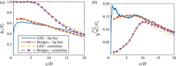
. The details of numerical methodology and grid independent studies have been discussed for various single stream jets by Naqavi et al. (Reference Naqavi, Wang, Tucker, Mahak and Strange2016), and the current grid distribution is the same as the validation case. To validate the LES simulation, we compared the calculated solution with Bridges experimental data (Bridges & Wernet Reference Bridges and Wernet2010). Both the mean flow and the turbulent fluctuation velocity profiles along the jet centreline and lip line are compared. The results are shown in figure 8(a,b). It can be seen that excellent agreement between the experimental and LES data is achieved for
 $x/D>2$
. The disagreement for
 $x/D<2$
is expected because the flow velocity is very sensitive to the inlet boundary conditions, and the inlet boundary conditions in experiments are very difficult to replicate.
Comparison of the jet mean and turbulent fluctuation velocity along centreline and lip line between the LES and experimental data.

The modal spectral correlation coefficient
 $\unicode[STIX]{x1D702}$
between the point at
 $r=1.8D$
and other points at different radial positions, all the points are at
 $x=6D$
.

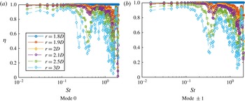
Figure 9 shows the modal spectral correlation coefficient between pressure fluctuations on a pair of coaxial circles at different radial positions using the LES data. The axial position is
 $x/D=6$
and the correlation coefficient is defined between the circle at
 $r=1.8D$
and other circles at
 $r=1.9D,2.0D,2.1D,2.5D,3.0D$
, respectively. Only modes
 $m=0$
and
 $m=\pm 1$
are shown, as the energy contained in mode
 $m$
reduces quickly as
 $m$
increases. This has been observed in several experimental studies – for example, the experimental work of Tinney, Glauser & Ukeiley (Reference Tinney, Glauser and Ukeiley2008a
) and Tinney & Jordan (Reference Tinney and Jordan2008). From figure 9 it appears that the coefficient is close to 1 at low frequencies for either mode 0 or (
 $\pm$
)1. This implies that the assumption of a dominant convection velocity is valid. The strong oscillation at high frequencies
 $St>0.2$
might well be due to acoustic contamination, particularly at large radial positions. However, as can be seen in the rest of this paper, the near-field pressure is only significant for frequencies satisfying
 $St<0.2$
. Therefore, it is reasonable to assign a fixed
 $U_{c}$
for each
 $m$
and
 $\unicode[STIX]{x1D714}$
for the near-field evanescent waves in the scattering model to be developed in the next subsection.
To determine these convection velocities, we consider the modal PSD of the near-field pressure fluctuation along the circle located at the axial position
 $x$
and radial position
 $r$
. Consider the correlation-based spectrum defined by
 $$\begin{eqnarray}\unicode[STIX]{x1D6F1}(\unicode[STIX]{x1D714},m;r)=\lim _{T\rightarrow \infty }\frac{\unicode[STIX]{x03C0}}{T}\left|\frac{\overline{\hat{p}(\unicode[STIX]{x1D714},m,r_{ref})\hat{p}^{\ast }(\unicode[STIX]{x1D714},m,r)}}{\sqrt{\overline{|\hat{p}(\unicode[STIX]{x1D714},m,r_{ref})|^{2}}}}\right|^{2},\end{eqnarray}$$
where
 $r_{ref}$
denotes the
 $r$
at a fixed reference point. Then using (2.34), we have
 $$\begin{eqnarray}\unicode[STIX]{x1D6F1}(\unicode[STIX]{x1D714},m;r)=P(\unicode[STIX]{x1D714},m)K_{m}^{2}\left(\sqrt{\bar{k}_{x}^{2}-k^{2}}r\right)\!.\end{eqnarray}$$
Hence the reduced power spectrum
 $$\begin{eqnarray}\overline{\unicode[STIX]{x1D6F1}}(\unicode[STIX]{x1D714},m;r)=\frac{\unicode[STIX]{x1D6F1}(\unicode[STIX]{x1D714},m;r)}{K_{m}^{2}\left(\sqrt{\bar{k}_{x}^{2}-k^{2}}r\right)}=P(\unicode[STIX]{x1D714},m)\end{eqnarray}$$
would be independent of
 $r$
and the reduced power spectra for any
 $r$
should collapse.
 $U_{c}$
can be evaluated from the collapsed radial decay rate
 $\unicode[STIX]{x1D6FE}$
.
The reduced power spectra of the near-field pressure fluctuation for points at
 $x=6D$
and different radial positions.

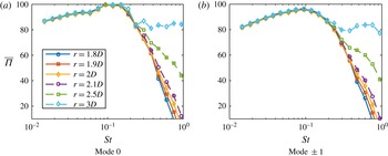
Figure 10 shows the reduced power spectra for different
 $r$
. An excellent data collapse is achieved for both mode
 $0$
and mode
 $(\pm )1$
. This is another strong piece of evidence that there does indeed exist a dominant local convection velocity for the near-field evanescent waves for each
 $m$
and
 $\unicode[STIX]{x1D714}$
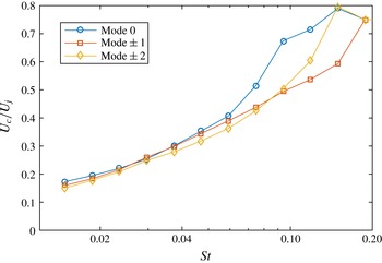
. The convection velocities for mode
 $0$
,
 $(\pm )1$
and
 $(\pm )2$
obtained in this way are shown in figure 11. As shown in figures 9 and 10, both the high spatial correlation and successful collapse of the reduced spectra are only valid for frequencies
 $St<0.2$
. Therefore, the convection velocities are only shown in this low-frequency regime. It can be seen that the convection velocity is much lower than
 $0.6U_{j}$
, which is heavily studied for instability waves at approximately
 $St=0.3$
. It is interesting to note that the frequency-dependent convection velocity curve obtained here is consistent with the finding of Kerhervé et al. (Reference Kerhervé, Fitzpatick and Jordan2006). From figure 11 we can find that the convection velocities for different azimuthal modes
 $m$
do not differ significantly from each other, especially for modes 0,
 $(\pm )1$
and
 $(\pm )2$
. This is consistent to the findings of Tinney, Ukeiley & Glauser (Reference Tinney, Ukeiley and Glauser2008b
) obtained using the proper orthogonal decomposition (POD) technique by analysing the pressure–velocity coupling. This fact is used in the following sections to simplify the scattering model.
The convection velocities at different frequencies for different mode
 $m$
obtained by collapsing spectra at different radial positions but at the same
 $x/D=6$
. Due to the dominant presence of acoustic waves at high frequencies, only the low-frequency regime is shown.

The reason for the loss in spatial correlation for the near-field pressure, and hence the failure of collapsing modal PSD, for
 $St>0.2$
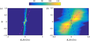
, is mostly due to the fact that the acoustic fluctuation is dominant in this frequency regime. To show this, we take the temporal and spatial Fourier transformations of the pressure along the straight line
 $r=3D,\,\unicode[STIX]{x1D703}=0$
and show the results in figure 12. From figure 12(a) it can be clearly seen that the wavenumber spectrum of the near-field pressure at high frequencies falls entirely inside the acoustic cone. This means that the pressure is effectively acoustic fluctuations rather than due to evanescent waves. Note that from figure 12(a) we have further confirmed that the convection velocity is a frequency-dependent quantity rather than a fixed constant between
 $0.6U_{j}$
and
 $0.8U_{j}$
. To better demonstrate this, the central region of figure 12(a) is expanded in figure 12(b). It is clear that at low frequencies the convection velocity is significantly less than
 $0.6U_{j}$
(the convection peaks on the right-hand side are below the line of
 $U_{c}=0.6U_{j}$
). It is worth noting that, due to the size limitation of the computational domain, the highest spatial resolution we achieved is
 $k_{x}D/(2\unicode[STIX]{x03C0})\approx 0.07$
. Therefore, at very low frequencies, e.g.
 $St<0.03$
, the convective peaks cannot be resolved. Also worth noting is that the convection peaks we show in this figure correspond to an overall convection velocity for the axial range
 $x=0$
to
 $14D$
; therefore, it is somewhat different from the local convection velocities obtained in figure 11.
The wavenumber spectrum of the near-field pressure along the line
 $r=3D,\,\unicode[STIX]{x1D703}=0$
: (a) full range; (b) zoomed-in central region. The green solid and blue dashed line correspond the convection velocities
 $U_{c}=c_{0}$
and
 $U_{c}=-c_{0}$
respectively; the dash-dotted magenta line corresponds to the convection velocity
 $U_{c}=0.6U_{j}$
.

2.2.2 Near-field pressure scattering
Using the conclusions we made about the near-field pressure in the preceding section, we develop a closed-form scattering model in this section. For a realistic wing–flap system, both the trailing edge and side edges of the wing and flap are present. We again adopt the same simplification used in developing the acoustic Green’s function: the wing and flap system are assumed to a semi-infinite flat plate with only a trailing edge. Due to the presence of the flat plate, we switch back to the Cartesian coordinates defined in figure 2 again. When the flat plate is sufficiently far away from the jet axis – for example, the perpendicular distance between the plate and the jet axis is greater than
 $2D$
– little change of the flow occurs due to the presence of the plate, and therefore the near-field evanescent waves, originating from hydrodynamic instability waves, can be found to be virtually same as that for an isolated jet (Bychkov & Faranosov Reference Bychkov and Faranosov2014). We can thus use the evanescent wave field for an isolated jet as the incident evanescent field for an installed jet. Assume the near-field pressure fluctuation is dominated by the evanescent wave of the first few modes, i.e. the pressure field can be written as
 $$\begin{eqnarray}p^{\prime }(\unicode[STIX]{x1D714},\boldsymbol{x})=\mathop{\sum }_{m=-N}^{N}\hat{p}(\unicode[STIX]{x1D714},m)K_{m}(\unicode[STIX]{x1D6FE}r)\,\text{e}^{-\text{i}k_{1}x_{1}}\,\text{e}^{\text{i}m\unicode[STIX]{x1D703}},\end{eqnarray}$$
where
 $\hat{p}(\unicode[STIX]{x1D714},m)$
denotes the magnitude of the pressure fluctuations of mode
 $m$
and frequency
 $\unicode[STIX]{x1D714}$
,
 $K_{m}$
the
 $m$
th order modified Bessel function of the second kind and the radius
 $r$
here is now defined as
 $\sqrt{x_{2}^{2}+(x_{3}+H)^{2}}$
, where
 $H$
is the distance between the jet centreline to the flat plate.
 $\unicode[STIX]{x1D6FE}$
, as defined earlier, denotes the decay rate
 $\sqrt{k_{1}^{2}-k^{2}}$
, where
 $k_{1}=\unicode[STIX]{x1D714}/U_{c}$
. The convection velocity
 $U_{c}$
(hence
 $k_{1}$
) is a function of
 $\unicode[STIX]{x1D714}$
and
 $m$
.
 $\unicode[STIX]{x1D703}$
is the azimuthal angle and
 $N$
is a small integer; for example, according to the LES data, we find
 $N=1$
is sufficient.
However, (2.39) is the solution of the reduced wave equation with a static ambient flow. In the presence of an uniform ambient flow of speed
 $U$
in the
 $x_{1}$
direction, (2.39) changes to
 $$\begin{eqnarray}p^{\prime }(\unicode[STIX]{x1D714},\boldsymbol{x})=\mathop{\sum }_{m=-N}^{N}\hat{p}(\unicode[STIX]{x1D714},m)K_{m}(\unicode[STIX]{x1D6FE}_{c}r)\,\text{e}^{-\text{i}k_{1}x_{1}}\,\text{e}^{\text{i}m\unicode[STIX]{x1D703}},\end{eqnarray}$$
where the convective radial decay rate
 $$\begin{eqnarray}\displaystyle \unicode[STIX]{x1D6FE}_{c}=\frac{\sqrt{(k_{1}\unicode[STIX]{x1D6FD}^{2}+kM)^{2}-k^{2}}}{\unicode[STIX]{x1D6FD}}. & & \displaystyle\end{eqnarray}$$
When the flat plate is directly above the jet, the hypothetical incident pressure that would exist on the lower surface of the plate if the plate were absent is
 $$\begin{eqnarray}\displaystyle & & \displaystyle p_{h}(\unicode[STIX]{x1D714},x_{1},x_{2})=\mathop{\sum }_{m=-N}^{N}\hat{p}(\unicode[STIX]{x1D714},m)K_{m}\left(\unicode[STIX]{x1D6FE}_{c}\sqrt{x_{2}^{2}+H^{2}}\right)\,\text{e}^{-\text{i}k_{1}x_{1}}\nonumber\\ \displaystyle & & \displaystyle \qquad \times \!\left(\mathop{\sum }_{k=0}^{[|m|/2]}C_{|m|}^{2k}(-1)^{k}\frac{H^{|m|-2k}x_{2}^{2k}}{\sqrt{x_{2}^{2}+H^{2}}^{|m|}}+\text{i}\operatorname{sgn}(m)\mathop{\sum }_{k=0}^{[|m|-1/2]}C_{|m|}^{2k+1}(-1)^{k}\frac{H^{|m|-2k-1}x_{2}^{2k+1}}{\sqrt{x_{2}^{2}+H^{2}}^{|m|}}\right)\!,\nonumber\\ \displaystyle & & \displaystyle\end{eqnarray}$$
where
 $[x]$
means taking the nearest integer that is not larger than
 $x$
, and
 $C_{m}^{n}$
is the binomial coefficient, which results from the use of de Moivre’s theorem. By making use of Fourier transformation, the hypothetical incident pressure can be expressed as a superposition of a series of plane waves, namely
 $$\begin{eqnarray}p_{h}(\unicode[STIX]{x1D714},x_{1},x_{2})=\mathop{\sum }_{m=-N}^{N}\int _{-\infty }^{\infty }\tilde{p}(\unicode[STIX]{x1D714},k_{2},m)\,\text{e}^{-\text{i}(k_{1}x_{1}+k_{2}x_{2})}\,\text{d}k_{2},\end{eqnarray}$$
where
 $$\begin{eqnarray}\displaystyle & & \displaystyle \hspace{-5.0pt}\tilde{p}(\unicode[STIX]{x1D714},k_{2},m)=\frac{1}{2\unicode[STIX]{x03C0}}\int _{-\infty }^{\infty }\hat{p}(\unicode[STIX]{x1D714},m)K_{m}\left(\unicode[STIX]{x1D6FE}_{c}\sqrt{x_{2}^{2}+H^{2}}\right)\,\text{e}^{\text{i}k_{2}x_{2}}\nonumber\\ \displaystyle & & \displaystyle \hspace{-5.0pt}\qquad \times \!\left(\mathop{\sum }_{k=0}^{[|m|/2]}C_{|m|}^{2k}(-1)^{k}\frac{H^{|m|-2k}x_{2}^{2k}}{\sqrt{x_{2}^{2}+H^{2}}^{|m|}}+\text{i}\operatorname{sgn}(m)\mathop{\sum }_{k=0}^{[|m|-1/2]}C_{|m|}^{2k+1}(-1)^{k}\frac{H^{|m|-2k-1}x_{2}^{2k+1}}{\sqrt{x_{2}^{2}+H^{2}}^{|m|}}\right)\,\text{d}x_{2}.\nonumber\\ \displaystyle & & \displaystyle\end{eqnarray}$$
Note that the real part of (2.42) is an even function of
 $x_{2}$
while the imaginary part is an odd function. Making use of this property and properties of Fourier transformation one can find that the
 $\hat{p}(\unicode[STIX]{x1D714},k_{2},m)$
can be evaluated analytically (Gradshteyn & Ryzhik Reference Gradshteyn and Ryzhik2007):
 $$\begin{eqnarray}\displaystyle & & \displaystyle \hspace{-5.0pt}\tilde{p}(\unicode[STIX]{x1D714},k_{2},m)=\frac{1}{\sqrt{2\unicode[STIX]{x03C0}}}\hat{p}(\unicode[STIX]{x1D714},m)\nonumber\\ \displaystyle & & \displaystyle \hspace{-5.0pt}\qquad \times \!\left\{\mathop{\sum }_{k=0}^{[|m|/2]}C_{|m|}^{2k}H^{-2k+1/2}\unicode[STIX]{x1D6FE}_{c}^{-|m|}\frac{\text{d}^{2k}}{\text{d}k_{2}^{2k}}\left[(\unicode[STIX]{x1D6FE}_{c}^{2}+k_{2}^{2})^{1/2|m|-1/4}K_{|m|-1/2}\left(H\sqrt{\unicode[STIX]{x1D6FE}_{c}^{2}+k_{2}^{2}}\right)\right]-\operatorname{sgn}(m)\right.\nonumber\\ \displaystyle & & \displaystyle \hspace{-5.0pt}\qquad \times \left.\mathop{\sum }_{k=0}^{[|m|-1/2]}C_{|m|}^{2k+1}H^{-2k+1/2}\unicode[STIX]{x1D6FE}_{c}^{-|m|}\frac{\text{d}^{2k}}{\text{d}k_{2}^{2k}}\left[k_{2}(\unicode[STIX]{x1D6FE}_{c}^{2}+k_{2}^{2})^{1/2|m|-3/4}K_{|m|-3/2}\left(H\sqrt{\unicode[STIX]{x1D6FE}_{c}^{2}+k_{2}^{2}}\right)\right]\right\}.\nonumber\\ \displaystyle & & \displaystyle\end{eqnarray}$$
For an incident pressure given by
 $\tilde{p}(\unicode[STIX]{x1D714},k_{2},m)\,\text{e}^{-\text{i}(k_{1}x_{1}+k_{2}x_{2})}$
, the scattered pressure on the lower surface of the flat plate can be found using the Schwarzschild technique as (Amiet Reference Amiet1976a
; Lyu, Azarpeyvand & Sinayoko Reference Lyu, Azarpeyvand and Sinayoko2016)
 $$\begin{eqnarray}p_{s}=\tilde{p}(\unicode[STIX]{x1D714},k_{2},m)\,\text{e}^{-\text{i}(k_{1}x_{1}+k_{2}x_{2})}\left((1+\text{i})E_{0}(-\unicode[STIX]{x1D707}x_{1})-1\right)\!,\end{eqnarray}$$
where
 $$\begin{eqnarray}\unicode[STIX]{x1D707}=k_{1}+\sqrt{k^{2}-k_{2}^{2}\unicode[STIX]{x1D6FD}^{2}}/\unicode[STIX]{x1D6FD}^{2}+kM/\unicode[STIX]{x1D6FD}^{2},\quad E_{0}(x)=\int _{0}^{x}\frac{\text{e}^{-\text{i}t}}{\sqrt{2\unicode[STIX]{x03C0}t}}\,\text{d}t.\end{eqnarray}$$
When the observer is located at
 $\boldsymbol{x}$
, routine application of the theory of Kirchhoff and Curle yields the far-field sound pressure (Amiet Reference Amiet1975; Lyu, Azarpeyvand & Sinayoko Reference Lyu, Azarpeyvand and Sinayoko2015; Lyu et al.
Reference Lyu, Azarpeyvand and Sinayoko2016)
 $$\begin{eqnarray}\displaystyle p_{f}(\unicode[STIX]{x1D714},\boldsymbol{x}) & = & \displaystyle (1+\text{i})\frac{\unicode[STIX]{x1D714}x_{3}}{\unicode[STIX]{x03C0}c_{0}S_{0}^{2}}\,\text{e}^{\text{i}k(Mx_{1}-S_{0})/\unicode[STIX]{x1D6FD}^{2}}\nonumber\\ \displaystyle & & \displaystyle \times \,\mathop{\sum }_{m=-N}^{N}\int _{-\infty }^{\infty }\frac{\displaystyle \sin \left[\left(k_{2}-k\frac{x_{2}}{S_{0}}\right)d/2\right]}{\displaystyle k_{2}-\frac{x_{2}}{S_{0}}}\frac{1}{\unicode[STIX]{x1D707}_{A}}\unicode[STIX]{x1D6E4}(c,\unicode[STIX]{x1D707},\unicode[STIX]{x1D707}_{A})\tilde{p}(\unicode[STIX]{x1D714},k_{2},m)\,\text{d}k_{2},\nonumber\\ \displaystyle & & \displaystyle\end{eqnarray}$$
where
 $c$
and
 $d$
are the chord and span of the finite plate respectively. Note when calculating (2.46) we assumed that the flat plate is semi-infinite. But when applying the theory of Kirchhoff and Curle to obtain (2.48) we used a finite plate of chord
 $c$
and span
 $d$
. The same approach was used by Amiet (Reference Amiet1976b
), and was found to be a good approximation provided the frequency is not too low (Roger & Moreau Reference Roger and Moreau2005). The properly bounded function
 $\unicode[STIX]{x1D6E4}$
in (2.48) is defined as
 $$\begin{eqnarray}\unicode[STIX]{x1D6E4}(x,\unicode[STIX]{x1D707},\unicode[STIX]{x1D707}_{A})=\text{e}^{\text{i}\unicode[STIX]{x1D707}_{A}x}E_{0}(\unicode[STIX]{x1D707}x)-\sqrt{\displaystyle {\displaystyle \frac{\unicode[STIX]{x1D707}}{\unicode[STIX]{x1D707}-\unicode[STIX]{x1D707}_{A}}}}E_{0}\left[(\unicode[STIX]{x1D707}-\unicode[STIX]{x1D707}_{A})x\right]+\frac{1}{1+\text{i}}(1-\text{e}^{\text{i}\unicode[STIX]{x1D707}_{A}x}),\end{eqnarray}$$
and
 $$\begin{eqnarray}\left.\begin{array}{@{}c@{}}\displaystyle S_{0}=\sqrt{x_{1}^{2}+\unicode[STIX]{x1D6FD}^{2}(x_{2}^{2}+x_{3}^{2})},\\ \displaystyle \unicode[STIX]{x1D707}_{A}=k_{1}+\frac{k}{\unicode[STIX]{x1D6FD}^{2}}\left(M-\frac{x_{1}}{S_{0}}\right)\!.\end{array}\right\}\end{eqnarray}$$
We note that normally aircraft wings have a large span-to-chord ratio, and
 $d$
can be quite large compared to the sound wavelength at the frequency of peak noise enhancement in the low-frequency regime, therefore we use
 $$\begin{eqnarray}\lim _{d\rightarrow \infty }\frac{\displaystyle \sin \left[\left(k_{2}-k\frac{x_{2}}{S_{0}}\right)d/2\right]}{\displaystyle \unicode[STIX]{x03C0}\left(k_{2}-k\frac{x_{2}}{S_{0}}\right)}=\unicode[STIX]{x1D6FF}\left(k_{2}-k\frac{x_{2}}{S_{0}}\right)\end{eqnarray}$$
to simplify (2.48) to
 $$\begin{eqnarray}p_{f}(\unicode[STIX]{x1D714},\boldsymbol{x})=(1+\text{i})\frac{\unicode[STIX]{x1D714}x_{3}}{c_{0}S_{0}^{2}}\mathop{\sum }_{m=-N}^{N}\frac{1}{\unicode[STIX]{x1D707}_{A}}\unicode[STIX]{x1D6E4}\left(c,\unicode[STIX]{x1D707}|_{k_{2}=k(x_{2}/S_{0})},\unicode[STIX]{x1D707}_{A}\right)\tilde{p}\left(\unicode[STIX]{x1D714},k\frac{x_{2}}{S_{0}},m\right)\!.\end{eqnarray}$$
The far-field sound power density spectrum can thus be obtained from
 $\unicode[STIX]{x1D6F7}_{N}(\unicode[STIX]{x1D714},\boldsymbol{x})=\lim _{T\rightarrow \infty }(\unicode[STIX]{x03C0}/T)\overline{p_{f}(\unicode[STIX]{x1D714},x)p_{f}^{\ast }(\unicode[STIX]{x1D714},x)}$
, i.e.:
 $$\begin{eqnarray}\displaystyle \unicode[STIX]{x1D6F7}_{N}(\unicode[STIX]{x1D714},\boldsymbol{x}) & = & \displaystyle 2\left[\frac{\unicode[STIX]{x1D714}x_{3}}{c_{0}S_{0}^{2}}\right]^{2}\mathop{\sum }_{m=-N}^{N}\mathop{\sum }_{m^{\prime }=-N}^{N}\!\left.\frac{\unicode[STIX]{x1D6E4}(c,\unicode[STIX]{x1D707}|_{k_{2}=k(x_{2}/S_{0})},\unicode[STIX]{x1D707}_{A})}{\unicode[STIX]{x1D707}_{A}}\right|_{m}\left.\frac{\unicode[STIX]{x1D6E4}^{\ast }(c,\unicode[STIX]{x1D707}|_{k_{2}=k(x_{2}/S_{0})},\unicode[STIX]{x1D707}_{A})}{\unicode[STIX]{x1D707}_{A}^{\ast }}\right|_{m^{\prime }}\nonumber\\ \displaystyle & & \displaystyle \times \,\lim _{T\rightarrow \infty }\frac{\unicode[STIX]{x03C0}}{T}\,\overline{\tilde{p}\left(\unicode[STIX]{x1D714},k\frac{x_{2}}{S_{0}},m\right)\tilde{p}^{\ast }\left(\unicode[STIX]{x1D714},k\frac{x_{2}}{S_{0}},m^{\prime }\right)}.\end{eqnarray}$$
It should be noted that (2.53) is due to the contribution of the scattered pressure only. In order to take the incident wave contribution into consideration, the term 1 in the last bracket on the right hand side of (2.49) defining the function
 $\unicode[STIX]{x1D6E4}(x,\unicode[STIX]{x1D707},\unicode[STIX]{x1D707}_{A})$
should be omitted (Amiet Reference Amiet1978).
Substituting (2.45) into the above equation, one finds the statistical term in (2.53) can be evaluated to be
 $$\begin{eqnarray}\displaystyle & & \displaystyle \hspace{-10.00002pt}\lim _{T\rightarrow \infty }\frac{\unicode[STIX]{x03C0}}{T}\,\overline{\tilde{p}\left(\unicode[STIX]{x1D714},k\frac{x_{2}}{S_{0}},m\right)\tilde{p}^{\ast }\left(\unicode[STIX]{x1D714},k\frac{x_{2}}{S_{0}},m^{\prime }\right)}=\frac{1}{2\unicode[STIX]{x03C0}}\unicode[STIX]{x1D6F1}(\unicode[STIX]{x1D714},m)\unicode[STIX]{x1D6FF}_{mm^{\prime }}\nonumber\\ \displaystyle & & \displaystyle \hspace{-10.00002pt}\qquad \times \!\left\{\mathop{\sum }_{k=0}^{[|m|/2]}C_{|m|}^{2k}H^{-2k+1/2}\unicode[STIX]{x1D6FE}_{c}^{-|m|}\frac{\text{d}^{2k}}{\text{d}k_{2}^{2k}}\left[(\unicode[STIX]{x1D6FE}_{c}^{2}+k_{2}^{2})^{1/2|m|-1/4}K_{|m|-1/2}\left(H\sqrt{\unicode[STIX]{x1D6FE}_{c}^{2}+k_{2}^{2}}\right)\right]-\operatorname{sgn}(m)\right.\nonumber\\ \displaystyle & & \displaystyle \hspace{-10.00002pt}\qquad \times \!\left.\;\mathop{\sum }_{k=0}^{[|m|-1/2]}C_{|m|}^{2k+1}H^{-2k+1/2}\unicode[STIX]{x1D6FE}_{c}^{-|m|}\frac{\text{d}^{2k}}{\text{d}k_{2}^{2k}}\left[k_{2}(\unicode[STIX]{x1D6FE}_{c}^{2}+k_{2}^{2})^{1/2|m|-3/4}K_{|m|-3/2}\left(H\sqrt{\unicode[STIX]{x1D6FE}_{c}^{2}+k_{2}^{2}}\right)\right]\right\}_{k_{2}=kx_{2}/S_{0}}^{2},\nonumber\\ \displaystyle & & \displaystyle\end{eqnarray}$$
where
 $\unicode[STIX]{x1D6F1}(\unicode[STIX]{x1D714},m)$
denotes the power spectrum of
 $m$
th order near-field evanescent waves. The spectrum could be obtained from simple models validated by experiments or LES simulations. Substituting (2.54) into (2.53) yields
 $$\begin{eqnarray}\displaystyle & & \displaystyle \hspace{-10.00002pt}\unicode[STIX]{x1D6F7}_{N}(\unicode[STIX]{x1D714},\boldsymbol{x})=\frac{1}{\unicode[STIX]{x03C0}}\left[\frac{\unicode[STIX]{x1D714}x_{3}}{c_{0}S_{0}^{2}}\right]^{2}\mathop{\sum }_{m=-N}^{N}\left|\frac{\unicode[STIX]{x1D6E4}(c,\unicode[STIX]{x1D707}|_{k_{2}=k(x_{2}/S_{0})},\unicode[STIX]{x1D707}_{A})}{\unicode[STIX]{x1D707}_{A}}\right|^{2}\unicode[STIX]{x1D6F1}(\unicode[STIX]{x1D714},m)\nonumber\\ \displaystyle & & \displaystyle \hspace{-10.00002pt}\qquad \times \!\left\{\mathop{\sum }_{k=0}^{[|m|/2]}C_{|m|}^{2k}H^{-2k+1/2}\unicode[STIX]{x1D6FE}_{c}^{-|m|}\frac{\text{d}^{2k}}{\text{d}k_{2}^{2k}}\left[(\unicode[STIX]{x1D6FE}_{c}^{2}+k_{2}^{2})^{1/2|m|-1/4}K_{|m|-1/2}\left(H\sqrt{\unicode[STIX]{x1D6FE}_{c}^{2}+k_{2}^{2}}\right)\right]-\operatorname{sgn}(m)\right.\nonumber\\ \displaystyle & & \displaystyle \hspace{-10.00002pt}\qquad \times \!\left.\mathop{\sum }_{k=0}^{[|m|-1/2]}C_{|m|}^{2k+1}H^{-2k+1/2}\unicode[STIX]{x1D6FE}_{c}^{-|m|}\frac{\text{d}^{2k}}{\text{d}k_{2}^{2k}}\left[k_{2}(\unicode[STIX]{x1D6FE}_{c}^{2}+k_{2}^{2})^{1/2|m|-3/4}K_{|m|-3/2}\left(H\sqrt{\unicode[STIX]{x1D6FE}_{c}^{2}+k_{2}^{2}}\right)\right]\vphantom{\mathop{\sum }_{k=0}^{[|m|-1/2]}}\right\}_{k_{2}=kx_{2}/S_{0}}^{2}.\nonumber\\ \displaystyle & & \displaystyle\end{eqnarray}$$
Equation (2.55) is the generic form of near-field scattering model. However, further simplifications can be made in practical cases. First, if we assume that the fluctuation is symmetric with respect to
 $m$
, i.e.
 $\unicode[STIX]{x1D6F1}(\unicode[STIX]{x1D714},m)=\unicode[STIX]{x1D6F1}(\unicode[STIX]{x1D714},-m)$
, (2.55) can be further simplified to
 $$\begin{eqnarray}\displaystyle & & \displaystyle \hspace{-13.00005pt}\unicode[STIX]{x1D6F7}_{N}(\unicode[STIX]{x1D714},\boldsymbol{x})=\frac{1}{\unicode[STIX]{x03C0}}\left[\frac{\unicode[STIX]{x1D714}x_{3}}{c_{0}S_{0}^{2}}\right]^{2}\mathop{\sum }_{m=0}^{N}\left|\frac{\unicode[STIX]{x1D6E4}(c,\unicode[STIX]{x1D707}|_{k_{2}=k(x_{2}/S_{0})},\unicode[STIX]{x1D707}_{A})}{\unicode[STIX]{x1D707}_{A}}\right|^{2}\unicode[STIX]{x1D6F1}_{s}(\unicode[STIX]{x1D714},m)\nonumber\\ \displaystyle & & \displaystyle \hspace{-15.00002pt}\qquad \times \!\left\{\left(\mathop{\sum }_{k=0}^{[|m|/2]}C_{|m|}^{2k}H^{-2k+1/2}\unicode[STIX]{x1D6FE}_{c}^{-|m|}\frac{\text{d}^{2k}}{\text{d}k_{2}^{2k}}\left[(\unicode[STIX]{x1D6FE}_{c}^{2}+k_{2}^{2})^{1/2|m|-1/4}K_{|m|-1/2}\left(H\sqrt{\unicode[STIX]{x1D6FE}_{c}^{2}+k_{2}^{2}}\right)\right]\right)^{2}\right.\nonumber\\ \displaystyle & & \displaystyle \hspace{-15.00002pt}\qquad +\!\left.\left(\mathop{\sum }_{k=0}^{[|m|-1/2]}C_{|m|}^{2k+1}H^{-2k+1/2}\unicode[STIX]{x1D6FE}_{c}^{-|m|}\frac{\text{d}^{2k}}{\text{d}k_{2}^{2k}}\left[k_{2}(\unicode[STIX]{x1D6FE}_{c}^{2}+k_{2}^{2})^{1/2|m|-3/4}K_{|m|-3/2}\left(H\sqrt{\unicode[STIX]{x1D6FE}_{c}^{2}+k_{2}^{2}}\right)\right]\vphantom{\mathop{\sum }_{k=0}^{[|m|-1/2]}}\right)^{2}\right\}_{k_{2}=kx_{2}/S_{0}},\hspace{-10.00002pt}\nonumber\\ \displaystyle & & \displaystyle\end{eqnarray}$$
where
 $\unicode[STIX]{x1D6F1}_{s}(\unicode[STIX]{x1D714},m)$
is the
 $m$
th single-sided modal power spectral density, i.e.
 $\unicode[STIX]{x1D6F1}_{s}(\unicode[STIX]{x1D714},m)=\unicode[STIX]{x1D6F1}(\unicode[STIX]{x1D714},m)+\unicode[STIX]{x1D6F1}(\unicode[STIX]{x1D714},-m)$
for
 $m\neq 0$
. If we assume that only the
 $0$
and
 $1(-1)$
modes are significant, we can show that the far-field sound spectral density in the midspan plane (
 $x_{2}=0$
) is
 $$\begin{eqnarray}\displaystyle \unicode[STIX]{x1D6F7}_{N}(\unicode[STIX]{x1D714},\boldsymbol{x}) & {\approx} & \displaystyle \left[\frac{\unicode[STIX]{x1D714}x_{3}}{c_{0}S_{0}^{2}}\right]^{2}\left\{\left|\frac{\unicode[STIX]{x1D6E4}(c,\unicode[STIX]{x1D707},\unicode[STIX]{x1D707}_{A})}{\unicode[STIX]{x1D707}_{A}}\right|^{2}\unicode[STIX]{x1D6F1}_{s}(\unicode[STIX]{x1D714},0)\frac{\text{e}^{-2H\unicode[STIX]{x1D6FE}_{c}}}{2\unicode[STIX]{x1D6FE}_{c}^{2}}\right\}_{k_{2}=0,m=0}\nonumber\\ \displaystyle & & \displaystyle +\left\{\left|\frac{\unicode[STIX]{x1D6E4}(c,\unicode[STIX]{x1D707},\unicode[STIX]{x1D707}_{A})}{\unicode[STIX]{x1D707}_{A}}\right|^{2}\unicode[STIX]{x1D6F1}_{s}(\unicode[STIX]{x1D714},1)\frac{\text{e}^{-2H\unicode[STIX]{x1D6FE}_{c}}}{2\unicode[STIX]{x1D6FE}_{c}^{2}}\right\}_{k_{2}=0,m=1}.\end{eqnarray}$$
Let
 $\unicode[STIX]{x1D6F1}_{0}(\unicode[STIX]{x1D714},0)$
and
 $\unicode[STIX]{x1D6F1}_{0}(\unicode[STIX]{x1D714},1)$
denote the zeroth and first single-sided modal power spectral densities measured at the location of
 $r=r_{0}$
, then it follows that
 $\unicode[STIX]{x1D6F1}_{s}(\unicode[STIX]{x1D714},0)K_{0}^{2}(\unicode[STIX]{x1D6FE}_{c}r_{0})=\unicode[STIX]{x1D6F1}_{0}(\unicode[STIX]{x1D714},0)$
and
 $\unicode[STIX]{x1D6F1}_{s}(\unicode[STIX]{x1D714},1)K_{1}^{2}(\unicode[STIX]{x1D6FE}_{c}r_{0})=\unicode[STIX]{x1D6F1}_{0}(\unicode[STIX]{x1D714},1)$
. Note in (2.57),
 $\unicode[STIX]{x1D707}$
,
 $\unicode[STIX]{x1D707}_{A}$
and
 $\unicode[STIX]{x1D6FE}_{c}$
depend on the mode number
 $m$
, as the convection velocity (hence
 $k_{1}$
) can vary with
 $m$
. However, in § 2.2.1 we show that the convection velocities for mode
 $0$
and
 $(\pm )1$
do not differ significantly from each other, therefore (2.57) can be further simplified by assuming an averaged convection velocity profile
 $\overline{U}_{c}(\unicode[STIX]{x1D714})$
over the two modes, such that
 $$\begin{eqnarray}\displaystyle \unicode[STIX]{x1D6F7}_{N}(\unicode[STIX]{x1D714},\boldsymbol{x})\approx \left[\frac{\unicode[STIX]{x1D714}x_{3}}{c_{0}S_{0}^{2}}\right]^{2}\left\{\left|\frac{\unicode[STIX]{x1D6E4}(c,\unicode[STIX]{x1D707},\unicode[STIX]{x1D707}_{A})}{\unicode[STIX]{x1D707}_{A}}\right|^{2}\frac{\text{e}^{-2H\unicode[STIX]{x1D6FE}_{c}}}{2\unicode[STIX]{x1D6FE}_{c}^{2}}\left(\frac{\unicode[STIX]{x1D6F1}_{0}(\unicode[STIX]{x1D714},0)}{K_{0}^{2}(\unicode[STIX]{x1D6FE}_{c}r_{0})}+\frac{\unicode[STIX]{x1D6F1}_{0}(\unicode[STIX]{x1D714},1)}{K_{1}^{2}(\unicode[STIX]{x1D6FE}_{c}r_{0})}\right)\right\}_{k_{2}=0,U_{c}=\overline{U}_{c}(\unicode[STIX]{x1D714})}. & & \displaystyle \nonumber\\ \displaystyle & & \displaystyle\end{eqnarray}$$
When in the frequency range of interest where
 $K_{0}(\unicode[STIX]{x1D6FE}_{c}r_{0})$
and
 $K_{1}(\unicode[STIX]{x1D6FE}_{c}r_{0})$
do not differ from each other significantly (such as the case to be presented in the § 3), (2.58) can be estimated by
 $$\begin{eqnarray}\unicode[STIX]{x1D6F7}_{N}(\unicode[STIX]{x1D714},\boldsymbol{x})\approx \left[\frac{\unicode[STIX]{x1D714}x_{3}}{c_{0}S_{0}^{2}}\right]^{2}\left\{\left|\frac{\unicode[STIX]{x1D6E4}(c,\unicode[STIX]{x1D707},\unicode[STIX]{x1D707}_{A})}{\unicode[STIX]{x1D707}_{A}}\right|^{2}\frac{\text{e}^{-2H\unicode[STIX]{x1D6FE}_{c}}}{2\unicode[STIX]{x1D6FE}_{c}^{2}}\frac{\unicode[STIX]{x1D6F1}_{0}(\unicode[STIX]{x1D714})}{K_{0}^{2}(\unicode[STIX]{x1D6FE}_{c}r_{0})}\right\}_{k_{2}=0,U_{c}=\overline{U}_{c}(\unicode[STIX]{x1D714})},\end{eqnarray}$$
where
 $\unicode[STIX]{x1D6F1}_{0}(\unicode[STIX]{x1D714})$
is the single-sided spectrum of the incident near-field evanescent waves at
 $r=r_{0}$
, which can be easily measured using one microphone in an isolated-jet experiment. To ensure acoustic fluctuations to be negligible, one can choose
 $r_{0}$
to be small such that the microphone is sufficiently close to the jet. Since this spectrum varies with axial position, it makes more sense to put the microphone at the position where the trailing edge of the flat plate would be if a flat plate were to be present, i.e. the place where the incident wave is to be scattered.
We have now obtained the far-field sound due to the quadrupole sources, i.e.
 $\unicode[STIX]{x1D6F7}_{Q}(\boldsymbol{x},\unicode[STIX]{x1D714})$
as shown in (2.20), and the sound due to the interaction between the near-field evanescent wave and the trailing edge of the flat plate, i.e.
 $\unicode[STIX]{x1D6F7}_{N}(\boldsymbol{x},\unicode[STIX]{x1D714})$
as shown from (2.55) to (2.59), the total sound power spectra is therefore
 $$\begin{eqnarray}\unicode[STIX]{x1D6F7}(\boldsymbol{x},\unicode[STIX]{x1D714})=\unicode[STIX]{x1D6F7}_{Q}(\boldsymbol{x},\unicode[STIX]{x1D714})+\unicode[STIX]{x1D6F7}_{N}(\boldsymbol{x},\unicode[STIX]{x1D714}).\end{eqnarray}$$
It is useful to review the inputs of this model. First,
 $\unicode[STIX]{x1D6F7}_{Q}(\boldsymbol{x},\unicode[STIX]{x1D714})$
is the sound predicted using Lighthill’s acoustic analogy. The Green’s function is obtained analytically, and therefore the input of this part is the time-averaged flow statistics obtained from RANS. Secondly, the near-field scattering part, e.g.
 $\unicode[STIX]{x1D6F7}_{N}(\boldsymbol{x},\unicode[STIX]{x1D714})$
shown in (2.59), requires the one-point spectrum and the local convection velocity (varying with frequency as well) of the near-field pressure fluctuation of an isolated jet at the location where the trailing edge of the flat plate would be. It is worth mentioning that though we perform an LES study in this paper, it is mostly for validation purposes, and the hybrid model does not directly require the input of the LES (at least for the cases where the convection velocity curve still applies or is known from experiments or models of instability waves).
It is worth noting that though the new model requires the near-field pressure spectrum as an input, this requirement could be removed if the strength of the evanescent instability waves were predicted by modelling the growth and decay of the jet instability waves, as is common in instability theory. However, to apply that to a particular experiment requires data on the perturbations at the nozzle exit. That information was not available in the experiment of Head & Fisher (Reference Head and Fisher1976), but the near-field pressure was, and we have used that for validation. Therefore, in general, a prediction model independent of experimental measurement is possible for specified exit boundary conditions. Though we do not have that information about boundary conditions to follow this approach, the semi-analytical model developed in the paper is also very useful in both understanding the underlying physics and developing ideas to control it. For example, the near-field scattering model proposed in this paper is nothing more than a transfer function, which maps the input (near-field pressure) spectrum to the output (far-field sound) spectrum. The fact it works well (as shown in the next section) confirms the scattering mechanism of the installed jet noise, and therefore provides evidence of this new sound source as opposed to isolated jets. By studying this transfer function, we can also understand the transfer efficiency, i.e. at which frequency the scattering is most efficient. The identification of the sound source and the understanding of the scattering mechanism is essential for noise reduction methods.
It should also be noted that while the ambient flow is taken into consideration and the effect of source motion is accounted for by the model of the fourth-order space–time correlation function, the model for installed jet noise developed in this section does not account for the mean jet flow refraction effect. Though this means that the model cannot correctly predict the far-field sound at high frequencies, it should suffice for the sound at
 $90^{\circ }$
to the jet and for low frequencies. In the next section, we will use the model developed in this section to predict the installed jet noise spectrum, and the results will be compared against experimental measurements.
3 Results
In 1976, in order to study the acoustic characteristics of low-frequency enhancement of the installed jet noise and to identify the corresponding noise sources, Head & Fisher (Reference Head and Fisher1976) presented a series of experimental results of the low-frequency augmentation of the jet noise with the close presence of a solid shield (flat plate), as shown in figure 13. There was no ambient flow, so
 $M=0$
. The experiment was carried out with a cold, subsonic, round jet (
 $D=1$
inch) at
 $M_{0}=0.5$
, the separation distance between the plate and the jet centreline
 $H=3D$
, and the distance between the trailing edge of the flat plate and the jet nozzle
 $L=6D$
. The far-field spectra for both isolated and installed jet noise were measured, and the microphone was located in the plane that is perpendicular to the rigid shield, but at
 $90^{\circ }$
,
 $45^{\circ }$
and
 $30^{\circ }$
to the jet centreline, respectively, on both the shielded and reflected sides. Since the rigid shield used in the experiment was placed sufficiently away from the jet, it can be expected to have little effect on the jet flow. Thus, in this section we use the two-part model, together with the inputs from axisymmetric jet flow field obtained in the preceding section, to calculate both the isolated and installed jet noise spectra. In the Lighthill acoustic analogy part,
 $\unicode[STIX]{x1D6F7}_{Q}(\boldsymbol{x},\unicode[STIX]{x1D714})$
, the turbulent statistics is obtained from the RANS calculation. In the near-field scattering part, we use the approximated (2.59) to calculate
 $\unicode[STIX]{x1D6F7}_{N}(\boldsymbol{x},\unicode[STIX]{x1D714})$
, and the spectrum of the near-field evanescent waves at the trailing-edge position was experimentally measured. But the local convection velocity at this point makes use of the averaged frequency-dependent velocity obtained from the aforementioned LES study. The results based on the new model are then compared with the experimental results.
The schematic of the experiment of Head & Fisher (Reference Head and Fisher1976). The separation distance between the flat plate and the jet centreline
 $H=3D$
, the distance between the trailing edge of the flat plate and the jet nozzle
 $L=6D$
.

3.1 Installed jet with acoustic scattering of Lighthill’s quadrupole sources
To demonstrate the existence of the additional near-field scattering mechanism for installed jet noise, the prediction of the far-field sound power spectrum with only the contribution of Lighthill’s quadrupole sources, i.e.
 $\unicode[STIX]{x1D6F7}_{Q}(\boldsymbol{x},\unicode[STIX]{x1D714})$
, is presented first. The predictions are compared with the experimental results.
Comparison between experimental measurements with model predictions for the far-field sound power spectrum in
 $1/3$
octaves for the installed jet with only the contribution of Lighthill’s quadrupole sources.

Figure 14(a) shows the sound power spectra at
 $90^{\circ }$
to the jet on the shielded side. The isolated sound spectra are also presented. As can be seen, the predicted spectrum for an isolated jet has an excellent agreement with experimental results. This shows that the RANS calculation and the fourth-order correlation model indeed work well. However, the predicted spectrum for an installed jet does not agree well with the experimental result. In particular, the predicted spectrum fails to capture the low-frequency amplification. The reason is because we have not yet incorporated the near-field scattering mechanism, which will be shown to account for such a noise intensification. The discrepancy at high frequencies, however, is in fact expected, since the jet refraction effect must be accounted for in order to correctly predict the shielding effect of the flat plate.
The noise spectra at
 $45^{\circ }$
and
 $30^{\circ }$
to the jet are shown in figures 14(b) and 14(c), respectively. The predicted spectra for isolated jet noise continues to agree well with experiment at low frequencies. But discrepancies start to appear at high frequencies, because the jet mean-flow refraction effect cannot be ignored at these angles. For the installed jet noise, the low-frequency enhancement at low frequencies at
 $45^{\circ }$
still fails to be captured, and the agreement at high frequencies is also affected by the refraction effect of the jet mean flow. But the prediction does indeed give some of the correct qualitative behaviour.
Figure 14(d) shows the noise power spectra predicted at
 $90^{\circ }$
on the reflected side. For installed jet noise spectra, despite the low-frequency discrepancies, the agreement at high frequencies is in fact very good. This indicates that the high-frequency reflection effect can be correctly captured at
 $90^{\circ }$
to the jet. Figures 14(e) and 14(f) present the noise spectra at
 $45^{\circ }$
and
 $30^{\circ }$
, respectively. For installed jet noise, despite the large discrepancies caused by the jet refraction effect, it is found that the qualitative behaviour of the noise increase due to the flat plate observed at high frequencies is correctly predicted. This suggests that if the refraction effect were to be included, the model would be able to give much better agreement with the experiment at high frequencies. It is worth noting that, at all the different observer angles, the low-frequency amplification cannot be captured, and this suggests that the near-field scattering mechanism is responsible for the low-frequency noise alteration.
3.2 Installed noise with two source mechanisms
From figures 14(a) to 14(f), it has been found that the noise spectrum predicted by incorporating only the contribution of the scattering of the Lighthill’s quadrupole sources cannot correctly model installed jet noise. In this part of this section, the contribution of the near-field scattering, i.e.
 $\unicode[STIX]{x1D6F7}_{N}(\boldsymbol{x},\unicode[STIX]{x1D714})$
described in § 2.2, is added. As mentioned above, the convection velocity of the near-field evanescent wave obtained by examining the radial decay rate using the LES data is used. We use the averaged convection velocity profile
 $\overline{U}_{c}(\unicode[STIX]{x1D714})$
obtained by averaging over modes
 $0$
and
 $(\pm )1$
. By combining the frequency-dependent convection velocity
 $\overline{U}_{c}(\unicode[STIX]{x1D714})$
and the experimentally measured near-field spectrum, the predicted far-field sound spectra at different angles are compared with experiments.
Comparison between experimental measurements with model predictions for the far-field sound power spectrum in
 $1/3$
octaves for the installed jet with two source mechanisms.

The sound spectra for both isolated and installed jets on the shielded side are shown in figures 15(a) to 15(c). As the spectra for isolated jet are identical to those shown in figure 14, we will focus only on the installed spectra hereafter. The predicted noise spectra at
 $90^{\circ }$
to the jet on the shielded side are presented in figure 15(a). It can be seen that very good agreement at low frequencies was achieved between the predicted and experimental results. A few reasons can be guessed to account for the slight under-prediction near the peak frequencies. First, it can be due to the slight error of estimated convection velocity, since the scattering is highly sensitive to this quantity. An experimental error is also possible: since the near-field pressure decays exponentially in the radial direction, a small misalignment of
 $2$
mm, for example, can cause a PSD change of up to
 $2$
dB. Given the solid shield used in the experiment can easily have a thickness of
 $2$
mm, the error could have been easily introduced. The sound spectra predicted at
 $45^{\circ }$
to the jet are shown in figure 15(b). Comparing with figure 14(b), where not all the low-frequency enhancement is captured, figure 15(b) does indeed better agree with the experimental results at low frequencies. Similarly, the sound spectra at
 $30^{\circ }$
is shown in figure 15(c), and the agreement with experimental results is good. As mentioned in the preceding subsection, the high-frequency sound is not predicted quantitatively, due to the mean-flow refraction effect, but the qualitative behaviours are successfully captured.
Figure 15(d–f) show the comparisons on the reflected side. As can be seen from figure 15(d), the agreement is similar to that at
 $90^{\circ }$
on the shielded side. The low-frequency enhancement is dominated by the near-field scattering, while the high-frequency amplification is due to the pure reflection effect, which is correctly captured using Lighthill’s quadrupole sources. The agreement at
 $45^{\circ }$
and
 $30^{\circ }$
to the jet is very similar to that on the shielded side. In particular, at
 $45^{\circ }$
the model prediction agrees better with experimental results. The high-frequency deviation, as already mentioned for the isolated jet, is caused by the refraction effect of the jet mean flow.
Even though overall good agreement between the model predictions and the experiment results at different observer angles is achieved at low frequencies, it should be noted that the high-frequency sound at low observer angles cannot be predicted correctly due to the jet refraction effect. A more accurate model aiming to include this effect is desired, and will form part of our future work.
4 Conclusion
This paper develops a low-order model to predict installed jet noise. The model starts with the development of a half-plane scattering Green’s function. The Green’s function is then used to solve the Lighthill’s acoustic analogy equation together with a model for the Lighthill’s quadrupole sources and the mean-flow data obtained by performing RANS calculations. The additional sound source due to near-field evanescent wave scattering is accounted for by developing a trailing-edge scattering model using Amiet’s approach. Therefore, the resulting far-field sound consists of the sum of contributions from two source mechanisms: Lighthill’s quadrupole sources and the near-field evanescent wave scattering. Finally, the proposed model is validated against experimental measurements.
It is found that when a solid shield (either a wing or a flat plate) is sufficiently far away from the jet, e.g. when the perpendicular distance between the shield and jet axis
 $H$
is greater than
 $2D$
, the noise at low frequencies (
 $St<0.2$
) due to Lighthill’s quadrupole sources is hardly affected by the presence of the solid shield. For high frequencies, however, the far-field sound due to quadrupole sources is either efficiently shielded at
 $90^{\circ }$
to the jet on the shielded side, or enhanced by approximately
 $3$
dB at
 $90^{\circ }$
to the jet on the reflected side. The sound from the quadrupole sources is also significantly refracted by the jet mean flow for the
 $M_{0}=0.5$
jet considered. Thus, at low observer angles, where the refraction effect is significant, only qualitatively agreement is achieved.
It is shown that the significant low-frequency noise enhancement observed in installed jet experiments is due to the interaction between the near-field evanescent wave and the trailing edge of the solid shield near the jet. The evanescent wave is believed to originate from the Kelvin–Helmholtz instability mechanism. Using the averaged
 $\overline{U}_{c}(\unicode[STIX]{x1D714})$
obtained from LES and the measured near-field evanescent pressure spectrum at the position where the trailing edge of the flat plate would be, the near-field scattering model can successfully predict the noise spectra at various observer angles. The sound due to near-field scattering, however, is only significant at low frequencies and negligible at high frequencies.
As already mentioned, one limitation of the two-part model developed in this paper is that it does not account for the jet refraction effect, which is significant at low observer angels to the jet for high-frequency sound and non-negligible jet Mach numbers. Thus, even though the qualitative behaviour of the far-field sound at high frequencies due to the presence of the flat shield is successfully predicted, quantitative agreement is not achieved except for the spectrum at
 $90^{\circ }$
to the jet on the reflected side. Another limitation is that the solid shield is assumed to be semi-infinite in the proposed model, and thus the effect of its side edges is ignored.
Acknowledgements
The first author (B.L.) wishes to gratefully acknowledge the financial support co-funded by the Cambridge Commonwealth European and International Trust and the China Scholarship Council. The third author (I.N.) wishes to acknowledge the UK Turbulence Consortium (UKTC) for the high-performance computing time to carry out the LES simulation on ARCHER under EPSRC grant no. EP/L000261/1 and under a PRACE award on HERMIT.
Appendix A
Detailed expression for the directivity terms
 $D_{ij}^{k}$
are shown as follows,
 $$\begin{eqnarray}\displaystyle \hspace{-10.00002pt}D_{12}^{0}(y_{1},y_{3})=-\frac{\cos \bar{\unicode[STIX]{x1D703}}(-M+\cos \bar{\unicode[STIX]{x1D6FC}})}{\unicode[STIX]{x1D6FD}^{3}}\left(E(u_{R})\,\text{e}^{\text{i}(k/\unicode[STIX]{x1D6FD})\cos \bar{\unicode[STIX]{x1D6FE}}y_{3}}+E(u_{R^{\prime }})\,\text{e}^{-\text{i}(k/\unicode[STIX]{x1D6FD})\cos \bar{\unicode[STIX]{x1D6FE}}y_{3}}\right)\!,\hspace{10.00002pt} & & \displaystyle\end{eqnarray}$$
 $$\begin{eqnarray}\displaystyle D_{12}^{1}(y_{1},y_{3}) & = & \displaystyle -\frac{\text{i}\cos \bar{\unicode[STIX]{x1D703}}\,\text{e}^{\text{i}(\unicode[STIX]{x03C0}/4)}\sqrt{\sin \bar{\unicode[STIX]{x1D703}}}}{\unicode[STIX]{x1D6FD}^{2}\sqrt{2\unicode[STIX]{x03C0}}}\nonumber\\ \displaystyle & & \displaystyle \times \!\left(\text{e}^{-\text{i}u_{R}^{2}}\cos \frac{\bar{\unicode[STIX]{x1D711}}+\bar{\unicode[STIX]{x1D711}}_{0}}{2}\,\text{e}^{\text{i}(k\cos \bar{\unicode[STIX]{x1D6FE}}/\unicode[STIX]{x1D6FD})y_{3}}+\text{e}^{-\text{i}u_{R^{\prime }}^{2}}\cos \frac{\bar{\unicode[STIX]{x1D711}}-\bar{\unicode[STIX]{x1D711}}_{0}}{2}\,\text{e}^{-\text{i}(k\cos \bar{\unicode[STIX]{x1D6FE}}/\unicode[STIX]{x1D6FD})y_{3}}\right)\!,\nonumber\\ \displaystyle & & \displaystyle\end{eqnarray}$$
 $$\begin{eqnarray}\displaystyle D_{23}^{0}(y_{1},y_{3}) & = & \displaystyle \frac{-\text{cos}\,\bar{\unicode[STIX]{x1D703}}\cos \bar{\unicode[STIX]{x1D6FE}}}{\unicode[STIX]{x1D6FD}^{2}}\left(E(u_{R})\,\text{e}^{\text{i}(k/\unicode[STIX]{x1D6FD})\cos \bar{\unicode[STIX]{x1D6FE}}y_{3}}-E(u_{R^{\prime }})\,\text{e}^{-\text{i}(k/\unicode[STIX]{x1D6FD})\cos \bar{\unicode[STIX]{x1D6FE}}y_{3}}\right)\!,\end{eqnarray}$$
 $$\begin{eqnarray}\displaystyle D_{23}^{1}(y_{1},y_{3}) & = & \displaystyle \frac{\text{i}\cos \bar{\unicode[STIX]{x1D703}}\,\text{e}^{\text{i}(\unicode[STIX]{x03C0}/4)}\sqrt{\sin \bar{\unicode[STIX]{x1D703}}}}{\unicode[STIX]{x1D6FD}\sqrt{2\unicode[STIX]{x03C0}}}\nonumber\\ \displaystyle & & \displaystyle \times \!\left(\text{e}^{-\text{i}u_{R}^{2}}\sin \frac{\bar{\unicode[STIX]{x1D711}}+\bar{\unicode[STIX]{x1D711}}_{0}}{2}\,\text{e}^{\text{i}(k\cos \bar{\unicode[STIX]{x1D6FE}}/\unicode[STIX]{x1D6FD})y_{3}}-\text{e}^{-\text{i}u_{R^{\prime }}^{2}}\sin \frac{\bar{\unicode[STIX]{x1D711}}-\bar{\unicode[STIX]{x1D711}}_{0}}{2}\,\text{e}^{-\text{i}(k\cos \bar{\unicode[STIX]{x1D6FE}}/\unicode[STIX]{x1D6FD})y_{3}}\right)\!,\nonumber\\ \displaystyle & & \displaystyle\end{eqnarray}$$
 $$\begin{eqnarray}\displaystyle D_{11}^{0}(y_{1},y_{3}) & = & \displaystyle -\left(\frac{-M+\cos \bar{\unicode[STIX]{x1D6FC}}}{\unicode[STIX]{x1D6FD}^{2}}\right)^{2}\left(E(u_{R})\,\text{e}^{\text{i}(k/\unicode[STIX]{x1D6FD})\cos \bar{\unicode[STIX]{x1D6FE}}y_{3}}+E(u_{R^{\prime }})\,\text{e}^{-\text{i}(k/\unicode[STIX]{x1D6FD})\cos \bar{\unicode[STIX]{x1D6FE}}y_{3}}\right)\!,\end{eqnarray}$$
 $$\begin{eqnarray}\displaystyle D_{11}^{1}(y_{1},y_{3}) & = & \displaystyle -\frac{2\text{i}(-M+\cos \unicode[STIX]{x1D6FC})\,\text{e}^{\text{i}(\unicode[STIX]{x03C0}/4)}\sqrt{\sin \bar{\unicode[STIX]{x1D703}}}}{\unicode[STIX]{x1D6FD}^{3}\sqrt{2\unicode[STIX]{x03C0}}}\left(\text{e}^{-\text{i}u_{R}^{2}}\cos \frac{\bar{\unicode[STIX]{x1D711}}+\bar{\unicode[STIX]{x1D711}}_{0}}{2}\,\text{e}^{\text{i}(k\cos \bar{\unicode[STIX]{x1D6FE}}/\unicode[STIX]{x1D6FD})y_{3}}\right.\nonumber\\ \displaystyle & & \displaystyle \times \!\left.\left(1+\frac{\sin \bar{\unicode[STIX]{x1D703}}}{(-M+\cos \bar{\unicode[STIX]{x1D6FC}})}\cos \left(\frac{\bar{\unicode[STIX]{x1D711}}+\bar{\unicode[STIX]{x1D711}}_{0}}{2}\right)\cos \left(\frac{\bar{\unicode[STIX]{x1D711}}-\bar{\unicode[STIX]{x1D711}}_{0}}{2}\right)\right)\right.\nonumber\\ \displaystyle & & \displaystyle \left.+\,\text{e}^{-\text{i}u_{R^{\prime }}^{2}}\cos \frac{\bar{\unicode[STIX]{x1D711}}-\bar{\unicode[STIX]{x1D711}}_{0}}{2}\,\text{e}^{-\text{i}(k\cos \bar{\unicode[STIX]{x1D6FE}}/\unicode[STIX]{x1D6FD})y_{3}}\right.\nonumber\\ \displaystyle & & \displaystyle \times \!\left.\left(1+\frac{\sin \bar{\unicode[STIX]{x1D703}}}{(-M+\cos \bar{\unicode[STIX]{x1D6FC}})}\cos \left(\frac{\bar{\unicode[STIX]{x1D711}}+\bar{\unicode[STIX]{x1D711}}_{0}}{2}\right)\cos \left(\frac{\bar{\unicode[STIX]{x1D711}}-\bar{\unicode[STIX]{x1D711}}_{0}}{2}\right)\right)\right)\!,\end{eqnarray}$$
 $$\begin{eqnarray}\displaystyle D_{11}^{2}(y_{1},y_{3}) & = & \displaystyle -\frac{\text{e}^{\text{i}(\unicode[STIX]{x03C0}/4)}\sqrt{\sin \bar{\unicode[STIX]{x1D703}}}}{2\unicode[STIX]{x1D6FD}\sqrt{2\unicode[STIX]{x03C0}}}\left(\text{e}^{-\text{i}u_{R}^{2}}\cos \left(\bar{\unicode[STIX]{x1D711}}_{0}+\frac{\bar{\unicode[STIX]{x1D711}}+\bar{\unicode[STIX]{x1D711}}_{0}}{2}\right)\,\text{e}^{\text{i}(k\cos \bar{\unicode[STIX]{x1D6FE}}/\unicode[STIX]{x1D6FD})y_{3}}\right.\nonumber\\ \displaystyle & & \displaystyle \left.+\,\text{e}^{-\text{i}u_{R^{\prime }}^{2}}\cos \left(\bar{\unicode[STIX]{x1D711}}_{0}-\frac{\bar{\unicode[STIX]{x1D711}}-\bar{\unicode[STIX]{x1D711}}_{0}}{2}\right)\,\text{e}^{-\text{i}(k\cos \bar{\unicode[STIX]{x1D6FE}}/\unicode[STIX]{x1D6FD})y_{3}}\right)\!,\end{eqnarray}$$
 $$\begin{eqnarray}\displaystyle D_{33}^{0}(y_{1},y_{3}) & = & \displaystyle -\left(\frac{\cos \bar{\unicode[STIX]{x1D6FE}}}{\unicode[STIX]{x1D6FD}}\right)^{2}\left(E(u_{R})\,\text{e}^{\text{i}(k/\unicode[STIX]{x1D6FD})\cos \bar{\unicode[STIX]{x1D6FE}}y_{3}}+E(u_{R^{\prime }})\,\text{e}^{-\text{i}(k/\unicode[STIX]{x1D6FD})\cos \bar{\unicode[STIX]{x1D6FE}}y_{3}}\right)\!,\end{eqnarray}$$
 $$\begin{eqnarray}\displaystyle D_{33}^{1}(y_{1},y_{3}) & = & \displaystyle \frac{2\text{i}\cos \bar{\unicode[STIX]{x1D6FE}}\,\text{e}^{\text{i}(\unicode[STIX]{x03C0}/4)}\sqrt{\sin \bar{\unicode[STIX]{x1D703}}}}{\unicode[STIX]{x1D6FD}\sqrt{2\unicode[STIX]{x03C0}}}\left(\text{e}^{-\text{i}u_{R}^{2}}\sin \frac{\bar{\unicode[STIX]{x1D711}}+\bar{\unicode[STIX]{x1D711}}_{0}}{2}\,\text{e}^{\text{i}(k\cos \bar{\unicode[STIX]{x1D6FE}}/\unicode[STIX]{x1D6FD})y_{3}}\right.\nonumber\\ \displaystyle & & \displaystyle \times \!\left.\left(1-\frac{\sin \bar{\unicode[STIX]{x1D703}}}{\cos \bar{\unicode[STIX]{x1D6FE}}}\cos \left(\frac{\bar{\unicode[STIX]{x1D711}}-\bar{\unicode[STIX]{x1D711}}_{0}}{2}\right)\sin \left(\frac{\bar{\unicode[STIX]{x1D711}}+\bar{\unicode[STIX]{x1D711}}_{0}}{2}\right)\right)\right.\nonumber\\ \displaystyle & & \displaystyle \left.+\,\text{e}^{-\text{i}u_{R^{\prime }}^{2}}\sin \frac{\bar{\unicode[STIX]{x1D711}}-\bar{\unicode[STIX]{x1D711}}_{0}}{2}\,\text{e}^{-\text{i}(k\cos \bar{\unicode[STIX]{x1D6FE}}/\unicode[STIX]{x1D6FD})y_{3}}\right.\nonumber\\ \displaystyle & & \displaystyle \times \!\left.\left(1-\frac{\sin \bar{\unicode[STIX]{x1D703}}}{\cos \bar{\unicode[STIX]{x1D6FE}}}\cos \left(\frac{\bar{\unicode[STIX]{x1D711}}+\bar{\unicode[STIX]{x1D711}}_{0}}{2}\right)\sin \left(\frac{\bar{\unicode[STIX]{x1D711}}-\bar{\unicode[STIX]{x1D711}}_{0}}{2}\right)\right)\right)\!,\end{eqnarray}$$
 $$\begin{eqnarray}\displaystyle D_{33}^{2}(y_{1},y_{3}) & = & \displaystyle \frac{\unicode[STIX]{x1D6FD}\,\text{e}^{\text{i}(\unicode[STIX]{x03C0}/4)}\sqrt{\sin \bar{\unicode[STIX]{x1D703}}}}{2\sqrt{2\unicode[STIX]{x03C0}}}\left(\text{e}^{-\text{i}u_{R}^{2}}\cos \left(\bar{\unicode[STIX]{x1D711}}_{0}+\frac{\bar{\unicode[STIX]{x1D711}}+\bar{\unicode[STIX]{x1D711}}_{0}}{2}\right)\,\text{e}^{\text{i}(k\cos \bar{\unicode[STIX]{x1D6FE}}/\unicode[STIX]{x1D6FD})y_{3}}\right.\nonumber\\ \displaystyle & & \displaystyle \left.+\,\text{e}^{-\text{i}u_{R^{\prime }}^{2}}\cos \left(\bar{\unicode[STIX]{x1D711}}_{0}-\frac{\bar{\unicode[STIX]{x1D711}}-\bar{\unicode[STIX]{x1D711}}_{0}}{2}\right)\,\text{e}^{-\text{i}(k\cos \bar{\unicode[STIX]{x1D6FE}}/\unicode[STIX]{x1D6FD})y_{3}}\right)\!,\end{eqnarray}$$
 $$\begin{eqnarray}\displaystyle D_{13}^{0}(y_{1},y_{3}) & = & \displaystyle -\left(\frac{(-M+\cos \bar{\unicode[STIX]{x1D6FC}})\cos \bar{\unicode[STIX]{x1D6FE}}}{\unicode[STIX]{x1D6FD}^{3}}\right)\left(E(u_{R})\,\text{e}^{\text{i}(k/\unicode[STIX]{x1D6FD})\cos \bar{\unicode[STIX]{x1D6FE}}y_{3}}-E(u_{R^{\prime }})\,\text{e}^{-\text{i}(k/\unicode[STIX]{x1D6FD})\cos \bar{\unicode[STIX]{x1D6FE}}y_{3}}\right)\!,\nonumber\\ \displaystyle & & \displaystyle\end{eqnarray}$$
 $$\begin{eqnarray}\displaystyle D_{13}^{1}(y_{1},y_{3}) & = & \displaystyle \frac{2\text{i}(-M+\cos \bar{\unicode[STIX]{x1D6FC}})\,\text{e}^{\text{i}(\unicode[STIX]{x03C0}/4)}\sqrt{\sin \bar{\unicode[STIX]{x1D703}}}}{\unicode[STIX]{x1D6FD}^{2}\sqrt{2\unicode[STIX]{x03C0}}}\nonumber\\ \displaystyle & & \displaystyle \times \!\left(\text{e}^{-\text{i}u_{R}^{2}}\,\text{e}^{\text{i}(k\cos \bar{\unicode[STIX]{x1D6FE}}/\unicode[STIX]{x1D6FD})y_{3}}\left(\frac{1}{2}\sin \frac{\bar{\unicode[STIX]{x1D711}}+\bar{\unicode[STIX]{x1D711}}_{0}}{2}-\frac{\cos \bar{\unicode[STIX]{x1D6FE}}}{2(-M+\cos \bar{\unicode[STIX]{x1D6FC}})}\cos \frac{\bar{\unicode[STIX]{x1D711}}+\bar{\unicode[STIX]{x1D711}}_{0}}{2}\right.\right.\nonumber\\ \displaystyle & & \displaystyle \left.+\,\frac{\sin \bar{\unicode[STIX]{x1D703}}}{-M+\cos \bar{\unicode[STIX]{x1D6FC}}}\cos \left(\frac{\bar{\unicode[STIX]{x1D711}}-\bar{\unicode[STIX]{x1D711}}_{0}}{2}\right)\sin \left(\frac{\bar{\unicode[STIX]{x1D711}}+\bar{\unicode[STIX]{x1D711}}_{0}}{2}\right)\cos \left(\frac{\bar{\unicode[STIX]{x1D711}}+\bar{\unicode[STIX]{x1D711}}_{0}}{2}\right)\right)\nonumber\\ \displaystyle & & \displaystyle \left.+\,\text{e}^{-\text{i}u_{R^{\prime }}^{2}}\,\text{e}^{-\text{i}(k\cos \bar{\unicode[STIX]{x1D6FE}}/\unicode[STIX]{x1D6FD})y_{3}}\left(-\frac{1}{2}\sin \frac{\bar{\unicode[STIX]{x1D711}}-\bar{\unicode[STIX]{x1D711}}_{0}}{2}+\frac{\cos \bar{\unicode[STIX]{x1D6FE}}}{2(-M+\cos \bar{\unicode[STIX]{x1D6FC}})}\cos \frac{\bar{\unicode[STIX]{x1D711}}-\bar{\unicode[STIX]{x1D711}}_{0}}{2}\right.\right.\nonumber\\ \displaystyle & & \displaystyle \left.\left.-\,\frac{\sin \bar{\unicode[STIX]{x1D703}}}{-M+\cos \bar{\unicode[STIX]{x1D6FC}}}\cos \left(\frac{\bar{\unicode[STIX]{x1D711}}+\bar{\unicode[STIX]{x1D711}}_{0}}{2}\right)\sin \left(\frac{\bar{\unicode[STIX]{x1D711}}-\bar{\unicode[STIX]{x1D711}}_{0}}{2}\right)\cos \left(\frac{\bar{\unicode[STIX]{x1D711}}-\bar{\unicode[STIX]{x1D711}}_{0}}{2}\right)\right)\right)\!,\nonumber\\ \displaystyle & & \displaystyle\end{eqnarray}$$
 $$\begin{eqnarray}\displaystyle D_{13}^{2}(y_{1},y_{3}) & = & \displaystyle \frac{\text{e}^{\text{i}(\unicode[STIX]{x03C0}/4)}\sqrt{\sin \bar{\unicode[STIX]{x1D703}}}}{2\sqrt{2\unicode[STIX]{x03C0}}}\left(\text{e}^{-\text{i}u_{R}^{2}}\sin \left(\bar{\unicode[STIX]{x1D711}}_{0}+\frac{\bar{\unicode[STIX]{x1D711}}+\bar{\unicode[STIX]{x1D711}}_{0}}{2}\right)\,\text{e}^{\text{i}(k\cos \bar{\unicode[STIX]{x1D6FE}}/\unicode[STIX]{x1D6FD})y_{3}}\right.\nonumber\\ \displaystyle & & \displaystyle \left.+\,\text{e}^{-\text{i}u_{R^{\prime }}^{2}}\sin \left(\bar{\unicode[STIX]{x1D711}}_{0}-\frac{\bar{\unicode[STIX]{x1D711}}-\bar{\unicode[STIX]{x1D711}}_{0}}{2}\right)\,\text{e}^{-\text{i}(k\cos \bar{\unicode[STIX]{x1D6FE}}/\unicode[STIX]{x1D6FD})y_{3}}\right)\!.\end{eqnarray}$$