


Nomenclature
-
 $T_s$
-
Rolling torque on the hull with respect to the yoke, results in forward rolling motion of the robot
-
$T_p$
-
Pendulum torque on the pendulum with respect to the yoke, results in lateral motion of the robot
-
$r_p$
-
Distance between the pendulum’s center of mass and hull’s geometric center
-
$r_h$
-
Radius of the hull (spherical shell)
-
$r_y$
-
Distance between the yoke’s center of mass and hull’s geometric center
-
$\mathbf{G}$
-
Global inertial frame fixed to the ground
-
$\mathbf{Y}$
-
Frame attached to the yoke
-
$\mathbf{P}$
-
Frame attached to the pendulum
-
$\mathbf{H}$
-
Frame attached to the hull
-
$\phi$
-
Heading angle of the robot measured with respect to the
$X$
-axis of global frame
$\mathbf{G}$
. This angle characterizes the precession of the robot. -
$\theta$
-
Lean angle of the robot perpendicular to the heading direction. This angle characterizes the lateral oscillations or wobbling of the robot
-
$\psi$
-
Forward spin angle of the robot responsible for moving it forward or backwards. This angle characterizes the forward rolling of the robot.
-
$\beta$
-
Pendulum angle relative to the yoke
-
${^{\mathbf{A}}}{\mathbf{R}}_{\mathbf{B}}$
-
Rotation matrix of frame A with respect to frame B
-
$\vec {{^{{{\mathbf{A}}}}}\omega _{\mathbf{A}}}$
-
The angular velocity vector of frame A expressed in frame A
-
$\vec {{}^{{\mathbf{A}}}_{{\mathbf{B}}}r_{{\mathbf{P}}}}$
-
Position vector of a point P starting from the origin of coordinate frame B expressed in frame A
-
${\mathbf{Y}}_c$
-
Position vector corresponding to the center of mass of yoke
-
${\mathbf{H}}_c$
-
Position vector corresponding to the center of mass of hull
-
${\mathbf{P}}_c$
-
Position vector corresponding to the pendulum’s center of mass
-
${\mathbf{P}}_o$
-
Position vector corresponding to the origin of pendulum frame
-
$X, Z$
-
X and Z co-ordinates of the hull center along the global frame
${\mathbf{G}}(OXYZ)$
-
$\vec {{^{\mathbf{A}}}v_{\mathbf{P}}}$
-
Linear velocity vector of point P expressed in frame A
-
$K$
-
Kinetic energy of the system
-
$V$
-
Potential energy of the system
-
$m_B$
-
mass of a body B
-
${^{\mathbf{B}}}I_{\mathbf{B}}$
-
The mass moment of inertia matrix of a body B calculated in its own frame of reference
-
$\lambda _i$
-
Lagrange multipliers
-
$L$
-
Lagrangian
-
$\mathbf{x}$
-
State vector representing robot’s motion
-
$u$
-
Control input
-
$q$
-
Generalized coordinates
-
$Q$
-
Generalized forces
-
$A$
-
Amplitude of lateral oscillations
-
$\omega$
-
Frequency of lateral oscillations
-
$\rho$
-
Radius of curvature for a spherical robot moving in a circular trajectory with pure rolling
-
$y$
-
Control output
-
$K_{p,\,\dot {\psi }}$
-
Speed control gain
-
$K_{p,\,\beta }$
-
Proportional component of pendulum control gain
-
$K_{d,\,\beta }$
-
Derivative component of pendulum control gain
-
$K_{p,\,\dot {\theta }}$
-
Wobble control gain
-
$T_{p,\,\dot {\theta }}$
-
Wobble control component of pendulum torque
-
$T_{p,\,\beta }$
-
Pendulum control component of pendulum torque
-
$\dot {\theta }_{des}$
-
Desired value of the rate of change of lean angle
-
$\dot {\psi }_{des}$
-
Desired value of forward speed
-
$\beta _{des}$
-
Desired value of the pendulum’s angle
-
$\gamma , \delta$
-
Coefficients of a linear combination


1. Introduction
Spherical robots offer a distinct advantage by enclosing all electro-mechanical components within a protective shell, shielding them from harsh environments and external impacts. Their ball-shaped design gives them the ability to recover effortlessly from collisions, preventing entrapment in corners. Furthermore, recent advancements highlight pendulum-based designs as they possess inherent stability thanks to their shape [Reference Diouf, Belzile, Saad and St-Onge1], enabling them to regain equilibrium after disturbances. This characteristic proves invaluable in scenarios where they are thrown or fall from heights. These advantages make them ideal for a wide range of applications, including surveillance, reconnaissance, hazardous environment assessment, search and rescue, and planetary exploration [Reference Armour and Vincent2–Reference Zhan, Cai and Liu4]. Spherical robots also find purpose as therapeutic and educational tools for children with developmental disorders, implying usefulness outside terrestrial exploration [Reference Mizumura, Ishibashi, Yamada, Takanishi and Ishii5].
Despite these advantages, experimental studies have consistently reported the presence of lateral oscillations, commonly referred to as wobble, in pendulum-driven spherical robots operating at various pendulum angles [Reference Oumer and Ylikorpi6–Reference Dwaracherla, Thakar, Vachhani, Gupta, Yadav and Modi8]. Early work by Froberg and Smolic [Reference Froberg and Smolic9] identified this wobbling behavior and proposed a PID-based approach to mitigate tipping errors induced by pendulum motion. Similarly, Schroll [Reference Schroll10] developed a detailed model of a spherical robot actuated by a two-degree-of-freedom pendulum, demonstrating that steering via a fixed pendulum inclination leads to wobbly circular trajectories characterized by lateral oscillations and a time-varying radius of curvature. Although these oscillations are usually small in magnitude and therefore overlooked, they become critical in applications involving onboard cameras or sensors, where even minor deviations can degrade data quality. Consequently, suppressing wobble is essential for achieving reliable perception and improved navigational autonomy. This, in addition to improvements in perception with panoramic camera setups for real-time object detection [Reference Arif, Zhu, Mao and Tu11], makes spherical robots a very strong surveillance and exploration solution.
The control of spherical robots is inherently challenging due to their nonholonomic constraints, underactuated nature, and non-chained system structure [Reference Joshi, Banavar and Hippalgaonkar12–Reference Roozegar, Ayati and Mahjoob14]. These challenges become more pronounced in non-ideal environments such as inclined terrains, where maintaining stability and accurate motion control is significantly more difficult [Reference Lin, Li, Huo and Wang15]. A variety of advanced control strategies have been proposed to address these challenges. For instance, recurrent neural network-based controllers have been developed to handle uncertainties and actuator saturation [Reference Chen, Beigi, Yousefpour, Rajaee, Jahanshahi, Bekiros, Martinez and Chu16], while reinforcement learning approaches have recently been explored for autonomous navigation [Reference Schröder, Garcia, Chacón, Montenegro, Marroquín, Farias, Dormido-Canto and Fabregas17]. Classical control techniques, including Lyapunov-based methods combined with neurodynamic approaches, have also been employed for trajectory tracking [Reference Cai, Zhan and Yan18]. In addition, adaptive high-speed sliding mode control strategies have been proposed to improve maneuverability under dynamic uncertainties [Reference Mao, Zhu, Wang, Li, Zhang, Zhang, Li, Zheng, Ma, Wu and Zhang19]. Direction and trajectory tracking control schemes for nonholonomic spherical robots have also been investigated to enhance tracking accuracy under constrained motion dynamics [Reference Liu, Wang, Guan, Hu, Zhang, Jin, Wang, Hao and Li20]. Furthermore, Hogan and Forbes [Reference Hogan and Forbes21] proposed a control framework for regulating heading and forward velocity in pendulum-actuated spherical robots. However, none of these approaches address the suppression of lateral oscillations.
Some studies have attempted to mitigate wobbling behavior, albeit with limited success. One approach [Reference Culebro, Aguirre and Munoz22] selects control outputs to regulate speed while minimizing pendulum oscillations; however, residual wobble persists, and unrestricted pendulum motion is often impractical due to spatial constraints within the shell. Sliding mode control strategies [Reference Liu, Sun and Jia23] have also been explored to regulate forward speed and lean angle, but they suffer from issues such as chattering and sensitivity to parameter tuning. In the context of Ballast Mass Fixed Axis designs, some works have focused on regulating lean angle using decoupled models [Reference Liu, Sun, Jia and Wang24], which neglect the coupling between linear and steering dynamics and therefore fail to eliminate wobble in practice. Other approaches employ system identification techniques to account for external disturbances [Reference Kamaldar, Mahjoob, Yazdi, Vahid-Alizadeh and Ahmadizadeh25] but do not address oscillations arising from intrinsic system dynamics during turning maneuvers. These limitations highlight the need for a modeling and control framework that explicitly captures and addresses the coupled dynamics responsible for wobble.
The motion capabilities of spherical robots are strongly influenced by their actuation mechanisms [Reference Crossley26, Reference Chase and Pandya27]. Existing designs can be broadly classified into direct driving methods [Reference Halme, Schonberg and Wang28], gravity-driven mechanisms (including pendulum-based systems [Reference Mahboubi, Fakhrabadi and Ghanbari29–Reference Balandin, Komarov and Osipov32] and gimbal-based configurations), angular momentum-driven systems utilizing flywheels [Reference Mao, Zhu, Tu, Zhang, Li, Zhang and Guo33], outer-shell deformation approaches [Reference Sheng, Xiang, Shouqiang and Kai34], and hybrid mechanisms [Reference Asiri, Khademianzadeh, Monadjemi and Moallem35]. Recent work [Reference Belzile and St-Onge36] has explored cylindrical pendulum configurations to improve spatial efficiency within the robot; these designs, however, do not explicitly address wobble observed at low speeds.
Corresponding to these diverse actuation strategies, a wide range of modeling approaches have been proposed to capture the complex dynamics of spherical robots. Early foundational work has established the nonholonomic nature and motion planning challenges of spherical robots through rigorous dynamic analysis [Reference Joshi and Banavar13]. First-order mathematical models based on rolling constraints and angular momentum conservation [Reference Bhattacharya and Agrawal46] provided initial insights into system behavior. More advanced formulations using Lagrangian methods and Euler angles have been widely adopted for modeling spherical motion on planar surfaces [Reference Rosen37, Reference Bloch38]. In addition, alternative formulations such as the Boltzmann–Hamel framework have been employed to derive dynamic models that more effectively capture nonholonomic constraints and system coupling [Reference Linsong and Zhan39]. While some studies simplify the problem by decoupling forward and steering dynamics [Reference Ylikorpi, Forsman, Halme and Saarinen40, Reference Liu, Sun and Jia41] or by modeling circular motion through gyroscopic precession [Reference Ylikorpi, Forsman and Halme42], others employ separate Euler–Lagrange formulations for different motion components [Reference Kayacan, Bayraktaroglu and Saeys43–Reference Cai, Zhan and Xi45]. However, these approaches often neglect the inherent coupling between lateral and longitudinal dynamics and consequently fail to capture the wobble observed in real systems. This gap motivates the need for a unified dynamic model that explicitly accounts for such coupling and enables systematic analysis and control of lateral oscillations.
The spherical robot.

Figure 1. Long description
The image shows two views of a spherical robot. The left view displays the assembled robot enclosed in a transparent hull, showcasing the internal components. The right view provides a detailed breakdown of the robot’s components, including a Raspberry Pi, camera, pendulum motor, yoke, yoke motor, battery, and pendulum. Each component is labeled to highlight its position and function within the spherical structure. The robot’s design emphasizes protection of internal components and stability, making it suitable for various applications such as surveillance, search and rescue, and educational tools.
This research focuses on a simulation-based analysis of a distinctive spherical robot with a yoke-pendulum design, illustrated in Figure 1. The yoke acts as a versatile platform for housing cameras, sensors, and electronic equipment. Two actuators drive the robot’s motion: one rotates the shell, enabling forward and backward movement, while the other rotates the pendulum relative to the yoke. The latter shifts the robot’s center of mass, hence steering the robot using gyroscopic effects. The pendulum’s swinging motion is restricted to the lower hemisphere, as the upper hemisphere accommodates sensors and other components on the yoke. The driving mechanism employed by this spherical robot is commonly referred to as the Ballast–Mass Fixed Axis Design, combining elements of gravity and angular momentum driving methods found in the literature.
This work makes the following contributions, which are organized into separate sections:
-
Section 2: Kinematic model and dynamic analysis of wobble present in the motion of a spherical robot by developing equations that account for the coupling of its forward and steering motions. This underactuated system is modeled using Lagrange-D’Alembert equations that take the frames using Euler angles and non-holonomic constraints into account with Lagrange multipliers. We also modify the model for conditions of slipping.
-
Section 3: A simplified version of the model for circular motion and formulation for the wobble amplitude, wobble frequency, radius of curvature, and the precession rate associated with the robot’s circular motion. The section concludes by comparing the system response generated by the actual model with that generated by the simplified model equations, demonstrating their similarity at different speeds.
-
Section 4: We propose a feedback linearization-based controller design for controlling the spherical robot’s heading direction via a turning maneuver while limiting its wobble and maintaining a stable and constrained pendulum motion.
-
Section 5: We demonstrate the versatility of the controller designed in the previous section, using a point-to-point navigation algorithm developed in our lab for both slip and no-slip conditions.
2. Modeling and dynamics
This section discusses the modeling of the pendulum-actuated spherical robot described in this work. The robot’s pendulum is mounted on the yoke at the geometric center of the hull through a motor that provides a torque
 $T_p$
. The yoke and the hull are connected through a motor mounted on the yoke. This motor rotates the hull by providing a torque
 $T_s$
. The center of mass of the hull and the yoke are at the geometric center of the hull, while the pendulum’s center of mass is at a distance
 $r_p$
from the geometric center. Using the Lagrange D’Alembert formulation, we determine the equations of motion for this system under both pure rolling and slip conditions.
2.1. Reference frames and Euler Angles
This work is based on four reference frames, as shown in Figure 2: a global inertial frame fixed to the ground (
 $\mathbf{G}$
) and the three frames attached to the yoke (
 $\mathbf{Y}$
), pendulum (
 $\mathbf{P}$
), and hull (
 $\mathbf{H}$
), respectively, with their origins at the geometric center of the hull. The yoke frame
 $\mathbf{Y}$
is defined to meet the following constraints: (1) The
 $z$
-axis of the yoke is always aligned with the
 $z$
-axis of the hull, and (2) The
 $x$
-axis of the yoke frame lies in the global
 $XZ$
-plane, i.e., it always remains parallel to the ground.
The orientation of the hull at any given instant is characterized by three
 $YXZ$
Euler angles
 $\phi$
,
 $\theta$
, and
 $\psi$
. The orientation of the pendulum requires another angle
 $\beta$
due to an additional degree of freedom. The transformation between frames happens as follows:
Frames and Euler angles (YXZ)

Figure 2. Long description
The image presents a detailed diagram illustrating the frames and Euler angles (YXZ) in a spherical robot design. It shows the global frame, hull frame, yoke frame, and pendulum frame, each with their respective axes labeled. The diagram includes various angles such as phi, theta, and psi, which represent the orientation of the robot in three-dimensional space. The global frame is depicted with X, Y, and Z axes, while the hull frame, yoke frame, and pendulum frame are shown with their respective axes and angles. The relationships between these frames and angles are visually represented with dashed and solid lines, indicating the rotational movements and orientations.
-
• Intermediate Frame (
$\mathbf{I}$
):
$\mathbf{G}$
is rotated along its
$Y$
-axis by angle
$\phi$
to obtain
$\mathbf{I}$
as shown in Figure 3a. -
• Yoke frame (
$\mathbf{Y}$
):
$\mathbf{I}$
is rotated along its local
$x$
-axis
$x_i$
by angle
$\theta$
to obtain
$\mathbf{Y}$
as shown in Figure 3b. -
• Pendulum frame (
$\mathbf{P}$
):
$\mathbf{Y}$
is rotated along its local
$x$
-axis
$x_y$
by angle
$\beta$
to obtain
$\mathbf{P}$
as shown in Figure 3c. Note that the angle made by the pendulum with the vertical axis
$Y$
is (
$\beta +\theta$
). -
• Hull frame (
$\mathbf{H}$
):
$\mathbf{Y}$
is rotated along its
$z$
-axis
$z_y$
by angle
$\psi$
to obtain
$\mathbf{H}$
as shown in Figure 3d.


Steps for obtaining the frames.

Figure 3. Long description
The diagram consists of four subfigures labeled (a) through (d), each depicting steps to obtain the different rotations and frames involved in the motion of a spherical robot. Subfigure (a) shows a top view rotation about the Y axis, involving the global frame and intermediate frame. Subfigure (b) presents a front view rotation about the xi axis, showing the intermediate frame and yoke frame. Subfigure (c) illustrates a front view rotation about the xy axis, involving the yoke frame and pendulum frame. Subfigure (d) depicts a side view rotation about the zy axis, showing the hull frame and yoke frame. Each subfigure includes labeled axes and angles, demonstrating the rotational relationships between different frames.
Careful design considerations are implemented in this system to avoid the gimbal lock problem. The yoke frame, obtained by rotating the intermediate frame along its local
 $x$
-axis, never reaches a vertical orientation where gimbal lock occurs. This is crucial to maintain optimal functionality, as a complete 90-degree tilt of the robot would result in a horizontal camera, limiting the field of view. Preventive measures have also been taken by restricting the pendulum’s angular displacement to the lower hemisphere of the robot and by housing all the electronics in the upper hemisphere. Furthermore, the control objectives and setpoints are meticulously chosen to minimize significant deviations from the mean lean angle, ensuring efficient operation of the system.
2.2. Robot kinematics
Rotation matrices mapping vectors from frames
 $\mathbf{Y}$
,
 $\mathbf{P}$
, and
 $\mathbf{H}$
to
 $\mathbf{G}$
are given by,
 ${{^{\mathbf{G}}}{\mathbf{R}}_{\mathbf{Y}}} = {R_y(\phi )} {R_x(\theta )}$
,
 ${{^{\mathbf{G}}}{\mathbf{R}}_{\mathbf{P}}} = {R_y(\phi )} {R_x(\theta )} {R_x(\beta )}$
, and
 ${{^{\mathbf{G}}}{\mathbf{R}}_{\mathbf{H}}} = {R_y(\phi )} {R_x(\theta )} {R_z(\psi )}$
.
The angular velocities of different frames are obtained to be:
 \begin{equation} \vec {{^{{\mathbf{Y}}}}\omega _{\mathbf{Y}}} = \begin{bmatrix} \dot {\theta } && \dot {\phi }\,\cos\!(\theta ) && -\dot {\phi }\,\sin\!(\theta ) \end{bmatrix}^\intercal {} \end{equation}
 \begin{equation} \vec {{^{\mathbf{P}}}\omega _{\mathbf{P}}} = \begin{bmatrix} \dot {\beta }+\dot {\theta } && \dot {\phi }\,\cos\!(\beta +\theta ) && -\dot {\phi }\,\sin\!(\beta +\theta ) \end{bmatrix}^\intercal {} \end{equation}
 \begin{equation} \vec {{^{\mathbf{H}}}\omega _{\mathbf{H}}} = \begin{bmatrix} \dot {\theta }\,\cos\!(\psi )\,+\,\dot {\phi }\,\cos\!(\theta )\,\sin\!(\psi ) \\ \dot {\phi }\,\cos\!(\psi )\,\cos\!(\theta )\,-\,\dot {\theta }\,\sin\!(\psi ) \\ \dot {\psi }\,-\,\dot {\phi }\,\sin\!(\theta ) \end{bmatrix} \end{equation}
The position vector corresponding to the center of mass of the yoke (
 ${\mathbf{Y}}_c$
) and the hull (
 ${\mathbf{H}}_c$
) as well as the origin of the pendulum frame (
 ${\mathbf{P}}_o$
) are
 \begin{equation} \vec {{}^{{\mathbf{G}}}_{{\mathbf{G}}}r_{{\mathbf{Y}}_c}} = \vec {{}^{{\mathbf{G}}}_{{\mathbf{G}}}r_{{\mathbf{H}}_c}} = \vec {{}^{{\mathbf{G}}}_{{\mathbf{G}}}r_{{\mathbf{P}}_o}} = \begin{bmatrix} X & r_h & Z \end{bmatrix}^\intercal {} \end{equation}
where
 $X$
and
 $Z$
are the coordinates of the hull center along the global frame
 ${\mathbf{G}}(OXYZ)$
, and
 $r_h$
is the radius of the sphere. Note that the origins of frames
 $\mathbf{Y, P, H}$
coincide at the center of the robot. The position vector corresponding to the pendulum’s center of mass is given by:
 \begin{equation} \vec {{}^{{\mathbf{G}}}_{{\mathbf{G}}}r_{{\mathbf{P}}_c}} = \vec {{}^{{\mathbf{G}}}_{{\mathbf{P}}}r_{{\mathbf{P}}_c}} + \vec {{}^{{\mathbf{G}}}_{{\mathbf{G}}}r_{{\mathbf{P}}_o}} \end{equation}
 \begin{equation} \vec {{}^{{\mathbf{G}}}_{{\mathbf{P}}}r_{{\mathbf{P}}_c}} = {^{\mathbf{G}}}{\mathbf{R}}_{\mathbf{P}} \vec {{}^{{\mathbf{P}}}_{{\mathbf{P}}}r_{{\mathbf{P}}_c}} \text{ and }\vec {{}^{{\mathbf{P}}}_{{\mathbf{P}}}r_{{\mathbf{P}}_c}} = \begin{bmatrix} 0 & -r_p & 0 \end{bmatrix}^\intercal {} \end{equation}
where
 ${\mathbf{P}}_c$
stands for the pendulum’s center of mass, and
 $r_p$
is the distance between
 ${\mathbf{P}}_c$
and
 ${\mathbf{P}}_o$
.
Differentiating the position vectors, the linear velocities of the center of mass of the hull (
 ${\mathbf{H}}_c$
), yoke (
 ${\mathbf{Y}}_c$
), and pendulum (
 ${\mathbf{P}}_c$
) are obtained as:
 \begin{equation} \vec {{^{\mathbf{G}}}v_{{\mathbf{H}}_c}} = \vec {{^{\mathbf{G}}}v_{{\mathbf{Y}}_c}} = \begin{bmatrix} \dot {X} & 0 & \dot {Z} \end{bmatrix}^\intercal {} \end{equation}
 \begin{equation} \vec {{^{\mathbf{G}}}v_{{\mathbf{P}}_c}} = \begin{bmatrix} \dot {X} \\ 0 \\ \dot {Z} \end{bmatrix} + \vec {{^{\mathbf{G}}}\omega _{\mathbf{P}}} \times {^{\mathbf{G}}}{\mathbf{R}}_{\mathbf{P}} \begin{bmatrix} 0 \\ -r_p \\ 0 \end{bmatrix} \end{equation}
The kinetic energy of the system can then be written as:
 \begin{equation} \begin{aligned} K &= K_L + K_A, \\ K_L &= \frac {1}{2} \Bigl ( m_h \bigl \lVert {^{\mathbf{G}}}\mathbf{v}_{\mathbf{H}_c} \bigr \rVert ^2 + m_y \bigl \lVert {^{\mathbf{G}}}\mathbf{v}_{\mathbf{Y}_c} \bigr \rVert ^2 + m_p \bigl \lVert {^{\mathbf{G}}}\mathbf{v}_{\mathbf{P}_c} \bigr \rVert ^2 \Bigr ), \\ K_A &= \frac {1}{2} \Bigl ( {^{\mathbf{H}}}\boldsymbol{\omega }_{\mathbf{H}}^{\mathsf{T}}\, {^{\mathbf{H}}}I_{\mathbf{H}}\, {^{\mathbf{H}}}\boldsymbol{\omega }_{\mathbf{H}} + {^{\mathbf{Y}}}\boldsymbol{\omega }_{\mathbf{Y}}^{\mathsf{T}}\, {^{\mathbf{Y}}}I_{\mathbf{Y}}\, {^{\mathbf{Y}}}\boldsymbol{\omega }_{\mathbf{Y}} + {^{\mathbf{P}}}\boldsymbol{\omega }_{\mathbf{P}}^{\mathsf{T}}\, {^{\mathbf{P}}}I_{\mathbf{P}}\, {^{\mathbf{P}}}\boldsymbol{\omega }_{\mathbf{P}} \Bigr ). \end{aligned} \end{equation}
where
 $m_j$
denotes the mass of body
 $\mathbf{J}$
, and
 ${^{\mathbf{J}}}I_{\mathbf{J}}$
denotes the mass moment of inertia matrix of body
 $\mathbf{J}$
expressed in its own reference frame. The spherical robot can be represented in an ideal way as a combination of primitive objects. The hull can be assumed to be a hollow sphere, the yoke to a disc, and the pendulum to a rod, with uniform distribution of mass. Following these assumptions,
 \begin{equation*} {^{\mathbf{H}}}I_{\mathbf{H}} = \operatorname {diag}\!(I_h, I_h, I_h), \quad {^{\mathbf{Y}}}I_{\mathbf{Y}} = \operatorname {diag}\!(I_y, 2 I_y, I_y), \quad {^{\mathbf{P}}}I_{\mathbf{P}} = \operatorname {diag}\!(I_p, 0, I_p), \end{equation*}
where
 \begin{equation*} I_h = \frac {2}{3} m_h r_h^2, \quad I_y = \frac {1}{4} m_y r_h^2, \quad I_p = \frac {1}{3} m_p r_p^2. \end{equation*}
From this we get the following upon expanding
 $K_L$
and
 $K_A$
as:
 \begin{equation} \begin{aligned} K_L &= \frac {1}{2} (m_h + m_y + m_p)(\dot {x}^2 + \dot {z}^2) + \frac {1}{2} m_p r_p^2 \left ( \dot {\phi }^2 \sin ^2\!(\theta + \beta ) + (\dot {\theta } + \dot {\beta })^2 \right ) \\ &\quad - m_p r_p \left ( \dot {x} \frac {d}{dt} \bigl ( \sin\!(\theta + \beta ) \sin \phi \bigr ) + \dot {z} \frac {d}{dt} \bigl ( \sin\!(\theta + \beta ) \cos \phi \bigr ) \right ),\\ K_A &= \frac {1}{2} \Big [ \left (\dot {\theta }^2 + \dot {\phi }^2 + \dot {\psi }^2 - 2 \dot {\phi } \dot {\psi } \sin \theta \right ) I_h \\ &\quad + \left (\dot {\theta }^2 + \dot {\phi }^2 (1 + \cos ^2 \theta ) \right ) I_y + \left ((\dot {\theta } + \dot {\beta })^2 + \dot {\phi }^2 \sin ^2\!(\theta + \beta ) \right ) I_p \Big ]. \end{aligned} \end{equation}
The Potential Energy of the system is given by
 \begin{equation} \begin{aligned} V &= m_p g \left ( \vec {{}^{\mathbf{G}}_{\mathbf{P}} \mathbf{r}_{\mathbf{P}_c}} \cdot [0\, 1\, 0]^\intercal \right ) + m_y g \left ( \vec {{}^{\mathbf{G}}_{\mathbf{Y}} \mathbf{r}_{\mathbf{Y}_c}} \cdot [0\, 1\, 0]^\intercal \right ) \\ &= - r_p m_p g \cos\!(\theta + \beta ). \end{aligned} \end{equation}
where the datum point for potential energy is chosen as the geometric center of the sphere.
In order to conduct a simulation, specific values have been assigned to the mass and dimensions of the hull, pendulum, and yoke. The mass of the hull has been set at 800 g, the mass of the pendulum at 200 g, and the mass of the yoke at 550 g. Similarly, the radius of the hull has been set to 12 cm, and the length of the pendulum has been set to 10 cm. These values have been chosen as inputs for the simulation to model as a representation of the prototype available in the lab on which previous experiments have been run. They have only been chosen to quantify the model, and the controller design isn’t limited to them. A mass and dimension optimization can be done as a future scope of this work, as it has no effect on the derivation of the mathematical model.
2.3. Non-holonomic constraints
The constraint of rolling without slipping is non-holonomic and is given by
 \begin{equation} \vec {{^{\mathbf{G}}}v_{\mathbf{H}}} = \vec {{^{\mathbf{G}}}\omega _{\mathbf{H}}} \times \vec {{^{\mathbf{G}}}r_{\mathbf{H}}} \end{equation}
where
 $\vec {{^{\mathbf{G}}}r_{\mathbf{H}}} = \begin{bmatrix} 0 & r_h & 0 \end{bmatrix}^\intercal$
denotes the vector (written in the global frame) between the stationary point on the hull, which is in contact with the ground and the sphere center. Eq. (12) is simplified further as
 \begin{equation} \dot {X} = r_h (\dot {\theta } \sin (\phi ) - \dot {\psi }\cos (\phi )\cos\!(\theta )) \end{equation}
 \begin{equation} \dot {Z} = r_h (\dot {\theta } \cos (\phi ) + \dot {\psi }\sin (\phi )\cos\!(\theta )) \end{equation}
These constraint equations are written in the form
 \begin{equation} a_1^\intercal \cdot \dot {q} = 0 \text{, } \quad a_2^\intercal \cdot \dot {q} = 0 \end{equation}
where generalized coordinates
 $q = \begin{bmatrix} X & Z & \phi & \theta & \psi & \beta \end{bmatrix} ^\intercal$
,
 $\vec {a_1}$
&
 $\vec {a_2}$
are:
 \begin{equation} \vec {a_1} = \begin{bmatrix} 1 &\quad 0 &\quad 0 &\quad -r_h sin(\phi ) &\quad r_h cos(\phi )\,cos(\theta ) &\quad 0 \end{bmatrix}^\intercal \end{equation}
 \begin{equation} \vec {a_2} = \begin{bmatrix} 0 &\quad 1 &\quad 0 &\quad -r_h cos(\phi ) &\quad -r_h sin(\phi )\,cos(\theta ) &\quad 0 \end{bmatrix}^\intercal \end{equation}
Next, the Lagrangian model is formulated utilizing the deduced constraints.
2.4. Lagrange D’Alembert equations
The Lagrange D’Alembert equations for non-holonomic systems are given by
 \begin{equation} \begin{aligned} \frac {d}{dt}\left (\frac {\partial L}{\partial \dot {q}}\right ) - \frac {\partial L}{\partial q} &= Q + \lambda _1 a_1 + \lambda _2 a_2, \\ Q &= \begin{bmatrix} 0 & 0 & 0 & 0 & T_s & T_p \end{bmatrix}^\intercal ,\\ L &= K_L + K_A - V \\ q &= \begin{bmatrix} X \quad Z \quad \phi \quad \theta \quad \psi \quad \beta \end{bmatrix}^\intercal \end{aligned} \end{equation}
where
 $T_s$
is the torque for forward rolling motion, and
 $T_p$
is the torque on the pendulum.
 $\lambda _1, \lambda _2$
are Lagrange multipliers;
 $a_1, a_2$
come from simplifying Eq. (15). Given that none of
 $K_L$
,
 $K_A$
, and
 $V$
are functions of
 $x$
or
 $z$
, and using Eqs. (13) and (14), we can break up Eq. (18) for each state
 $q$
into the following:
 \begin{equation} \begin{aligned} \frac {\partial L}{\partial x} &= 0, & \frac {\partial L}{\partial z} &= 0, \\ \implies \frac {d}{dt}\left (\frac {\partial L}{\partial \dot {x}}\right ) &= \lambda _1, & \frac {d}{dt}\left (\frac {\partial L}{\partial \dot {z}}\right ) &= \lambda _2 \\ \end{aligned} \end{equation}
Using Eq. (19), we can eliminate
 $\lambda _1, \lambda _2$
in the following equations.
 \begin{equation} \begin{aligned} \frac {d}{dt}\left (\frac {\partial L}{\partial \dot {\beta }}\right ) - \frac {\partial L}{\partial \beta } &= T_p, \end{aligned} \end{equation}
 \begin{equation} \begin{aligned} \frac {d}{dt}\left (\frac {\partial L}{\partial \dot {\theta }}\right ) - \frac {\partial L}{\partial \theta } &= -r_h\left (sin(\phi ) \lambda _1 + cos(\phi ) \lambda _2\right ), \end{aligned} \end{equation}
 \begin{equation} \begin{aligned} \frac {d}{dt}\left (\frac {\partial L}{\partial \dot {\psi }}\right ) - \frac {\partial L}{\partial \psi } &= T_s + r_h cos(\theta ) \left (cos(\phi ) \lambda _1 - sin(\phi ) \lambda _2\right ), \end{aligned} \end{equation}
 \begin{equation} \begin{aligned} \frac {d}{dt}\left (\frac {\partial L}{\partial \dot {\phi }}\right ) - \frac {\partial L}{\partial \phi } &= 0, \end{aligned} \end{equation}
Finally, the last two equations of motion come from the Eqs. (13) and (14) as shown below:
 \begin{equation} \begin{aligned} \frac {d}{dt}\left (a_1^\intercal \cdot \dot {q}\right ) = 0, \quad \quad \frac {d}{dt}\left (a_2^\intercal \cdot \dot {q}\right ) = 0 \end{aligned} \end{equation}
The system model that is formed using the Eqs. (20) to (24) can be represented as,
 \begin{equation} \mathbf{M}(q)\ddot {\mathbf{q}} + \mathbf{C}(q,\dot {q})\dot {\mathbf{q}} + \mathbf{g}(q) = \boldsymbol{\tau }, \end{equation}
where
 $\mathbf{M}(q)$
,
 $\mathbf{C}(q,\dot {q})$
,
 $\mathbf{g}(q)$
, and
 $\boldsymbol{\tau }$
are expanded in the Appendix (Section 7.1). Using elementary row operations on Eq. (25) expanded in the Appendix (Section 7.2) and representing the state vector
 $\mathbf{x}$
and control inputs
 $\mathbf{u}$
compactly as
 \begin{equation} \quad \mathbf{x} = \begin{bmatrix} \phi \quad \theta \quad \psi \quad \beta \quad X \quad Z \quad \dot {\phi } \quad \dot {\theta } \quad \dot {\psi } \quad \dot {\beta } \quad \dot {X} \quad \dot {Z} \end{bmatrix}^\intercal , \quad \mathbf{u} = \begin{bmatrix} T_s \quad T_p \end{bmatrix}^\intercal . \end{equation}
Eq. (25) can be simplified to give the control-affine form represented below:
 \begin{equation} \dot {\mathbf{x}} = \mathbf{f}(\mathbf{x}) + \mathbf{G}(\mathbf{x}) \mathbf{u}, \end{equation}
where
 \begin{equation*} \mathbf{f}(\mathbf{x}) = \begin{bmatrix} \dot {\phi } \\ \dot {\theta } \\ \dot {\psi } \\ \dot {\beta } \\ \dot {X} \\ \dot {Z} \\ f_7(\theta , \beta , \dot {\phi }, \dot {\theta }, \dot {\psi }, \dot {\beta }) \\ f_8(\theta , \beta , \dot {\phi }, \dot {\theta }, \dot {\psi }, \dot {\beta }) \\ f_9(\theta , \beta , \dot {\phi }, \dot {\theta }, \dot {\psi }, \dot {\beta }) \\ f_{10}(\theta , \beta , \dot {\phi }, \dot {\theta }, \dot {\psi }, \dot {\beta }) \\ f_{11}(\phi , \theta , \beta , \dot {\phi }, \dot {\theta }, \dot {\psi }, \dot {\beta }) \\ \,f_{12}(\phi , \theta , \beta , \dot {\phi }, \dot {\theta }, \dot {\psi }, \dot {\beta }) \end{bmatrix}, \quad \mathbf{G}(\mathbf{x}) = \begin{bmatrix} 0 & 0 \\ 0 & 0 \\ 0 & 0 \\ 0 & 0 \\ 0 & 0 \\ 0 & 0 \\ G_{7,1}(\theta , \beta ) & 0 \\ 0 & G_{8,2}(\theta , \beta ) \\ G_{9,1}(\theta , \beta ) & 0 \\ 0 & G_{10,2}(\theta , \beta ) \\ G_{11,1}(\phi , \theta , \beta ) & G_{11,2}(\phi , \theta , \beta ) \\ G_{12,1}(\phi , \theta , \beta ) & G_{12,2}(\phi , \theta , \beta ) \end{bmatrix}. \end{equation*}
Expanding each term of this model equation becomes very lengthy and reduces the readability of this article; hence, a detailed representation of the methodology is given in the appendix. This model exhibits coupling between the forward rolling and steering motions of the robot. The forward rolling motion is characterized by the forward spin angle
 $\psi$
and the heading angle
 $\phi$
, while the steering motion is characterized by the lean angle
 $\theta$
and the pendulum angle
 $\beta$
.
Analyzing the model equations reveals that the derivatives
 $\dot {\psi }$
and
 $\dot {\phi }$
appear in the expressions for the second derivatives
 $\ddot {\theta }$
and
 $\ddot {\beta }$
. This indicates that the steering motion depends on the current rates of change of the forward spin and heading angles. Conversely, the variables
 $\theta$
,
 $\beta$
, and their derivatives appear in the equations for
 $\ddot {\psi }$
and
 $\ddot {\phi }$
, showing that the forward motion is influenced by the lean and pendulum angles and their rates of change. Therefore, changes in the forward motion variables
 $\psi$
and
 $\phi$
impact the steering variables
 $\theta$
and
 $\beta$
, and vice versa.
Finally, note that the system is underactuated with only two control inputs,
 $T_s$
and
 $T_p$
, which limits the number of outputs that can be controlled.
2.5. Rolling with slipping
The deduced constraints in the previous subsection enforce that the hull of the robot rolls on the ground without slipping. However, this is idealistic; therefore, we have generalized this setup to rolling with slipping as well. The generalized force vector when considering friction as an external force is as follows:
 \begin{equation} Q_{slip} = \begin{bmatrix} f_x \\ f_z \\ 0 \\ - r_h (\,f_x sin(\phi ) + f_z cos(\phi )) \\ T_s - r_h cos(\theta ) (\,f_x cos(\phi ) - f_z sin(\phi )) \\ T_p \end{bmatrix} \end{equation}
Where
 $f_x$
and
 $f_z$
are the components of the friction force acting in the global
 $X$
and
 $Z$
directions, respectively, and
 $T_s$
and
 $T_p$
are the torques from the motors contributing to the forward angular velocity and the pendulum steering, respectively. From the Lagrangian formulation, we can deduce the values of
 $\lambda _1$
and
 $\lambda _2$
to be
 $f_x$
and
 $f_z$
, respectively.
Rolling with Slip may occur when the point of contact between the robot and the ground has relative motion between them or the force of friction required to maintain rolling is too high for the given surface. The friction model used for these simulations is the Coulomb friction model, and we demonstrate the effect of different coefficients of friction
 $\mu$
.
 \begin{equation*}F_{Coulumb} = \mu \times F_{Normal} \times sign(v_{poc})\end{equation*}
As we will see in Section 3, the system in steady-state circular motions stays well within the Coulomb model limit (
 $\mu F_{Normal}$
), and we will specifically study the robustness of the wobble controller designed in Section 4 to the case of slipping at low speeds, expressed in Figure 5b.
2.6. System response for a circular motion
The dynamics of the spherical robot described in Section 2.4 are simulated using the ODE15s solver built into MATLAB. Specifically, we have simulated the steady-state behavior of the robot rolling along a circular path. This configuration is attained when the pendulum’s angle and the robot’s forward speed are held constant and the remaining state variables are initialized as zero.
Our system analysis is conducted for relatively smaller pendulum angles so that the robot does not lean excessively during steering motion. A steep lean angle during the steering motion would laterally tilt the camera mounted on the robot. Hence, we focus our analysis on a pendulum’s swing of about 0
 $^{\circ }$
to 15
 $^{\circ }$
since this is a relatively small inclination. Within this range, simulations are roughly divided into two groups: Low Pendulum Angle (5
 $^{\circ }$
) and High Pendulum Angle (15
 $^{\circ }$
).
We have also classified the speeds of robot operation as either “Low Speed” or “High Speed.” In Figure 4, we show the system response for the robot’s center of mass as it moves forward at varying speeds while maintaining a pendulum angle of 15
 $^{\circ }$
. The circular paths that the robot follows are slightly wobbly due to oscillations in the robot’s lean angle
 $\theta$
. The deviations from a perfect circular path shown in Figure 4 are proportional to the amplitude of oscillations in lean angle.
We can see from Figure 4 that the robot’s wobbling is minimal when it is moving at a speed of 10 radians per second. At this speed, the robot follows a nearly smooth circular trajectory, as shown in Figure 5d. The magnitude of the mean value and amplitude of the lean angle is 1.76
 $^{\circ }$
for this case, which results in a total lean angle deviation of about 3.5
 $^{\circ }$
about the mean position. As this deviation is smaller than 5.73
 $^{\circ }$
(i.e. 0.1 rad), we can consider it to be a very small angular deviation. Therefore, for our simulations, we classify 10 radians per second as a high speed, as it results in relatively smaller values of wobbling.
Similarly, we classify 1 rad/s as a low speed because the effect of wobbling caused by center of mass perturbation is clearly visible in Figure 4. In this case, the corresponding behavior of lean angle (
 $\theta$
) is shown in Figure 5b, where the magnitude of the mean value and amplitude of the lean angle is 13.8
 $^{\circ }$
. This results in a total lean angle deviation of 27.62
 $^{\circ }$
about the mean position, which is very high. Such a high deviation can result in significantly shaky camera feedback, which is not desirable. Additionally, this deviation is well above the approximate small angle value of 20
 $^{\circ }$
, where small angle approximations are approximately valid.
Path followed by robot’s COM while moving forward at different speeds
 $|\dot {\psi }|$
with
 $\beta = 15^{\circ }$
.

Figure 4. Long description
The image is a four-part line graph that illustrates the path followed by the center of mass of the spherical robot as it moves in a circular motion at different speeds with a constant pendulum angle. Each subplot represents a different angular velocity: 1 radian per second, 2 radians per second, 5 radians per second, and 10 radians per second. The x-axis of each graph is labeled ’X (cm)’ and the y-axis is labeled ’-Z (cm)’. The paths are depicted as blue lines, showing the trajectory of the robot’s center of mass. The first graph shows a more lateral oscillations (wobble) at 1 radian per second, while the subsequent graphs display increasingly smoother and more circular paths as the forward velocity increases.
We further investigate the system response for the rate of change of heading angle
 $\dot {\phi }$
, rate of change of lean angle
 $\dot {\theta }$
, forward speed
 $\dot {\psi }$
, and lean angle
 $\theta$
by simulating the steady state circular motion of the robot with the following four configurations of pendulum angle
 $\beta$
and forward rolling speed
 $|\dot {\psi }|$
while in pure rolling as well as rolling with slip:

System response at various pendulum angles and forward speeds.

Figure 5. Long description
The image contains four sets of graphs, each set showing the system response under different conditions. Each set includes four graphs: roll rate, pitch rate, yaw rate, and pitch angle over time. The graphs compare pure rolling and rolling with slip. The first set shows the system response at a 5-degree angle and 1 radian per second speed. The second set shows the system response at a 15-degree angle and 1 radian per second speed. The third set shows the system response at a 5-degree angle and 10 radians per second speed. The fourth set shows the system response at a 15-degree angle and 10 radians per second speed. Each graph plots time in seconds on the x-axis and the respective rate or angle on the y-axis. The blue lines represent pure rolling, while the orange lines represent rolling with slip. The graphs illustrate how the system’s response varies with different angles and speeds, highlighting the differences between pure rolling and rolling with slip.
In order to facilitate the comparison of the figures, we have opted to use different scales for certain variables in each case. We kept a consistent scale for the
 $\theta$
variable over time, as this allowed for a relative comparison of the wobble values depicted in Figure 5a, 5b, 5c, and 5d. In each figure set, we scaled
 $\dot {\phi }$
,
 $\dot {\theta }$
, and
 $\dot {\psi }$
in the same way to enable a relative comparison of the angular velocities.
The system response in the figures shows two distinct ends. On one end, we see the lean angle exceeding the range in which it can be approximated as a small angle. For instance, at a rolling speed of 1 rad/sec and a pendulum angle of 15
 $^{\circ }$
, the lean angle can reach up to 30
 $^{\circ }$
in magnitude. If we were to go further on these sides of the configurations, the wobble would increase further. If the robot were to operate at speeds below 1 rad/s with the pendulum at a reasonable angle of 15
 $^{\circ }$
, it would cause an excessive tilt angle, with values exceeding 30
 $^{\circ }$
. This high tilt angle would cause the camera to tilt excessively in the sideways direction, resulting in a loss of camera field of view on the other side.
On the other end of the system response, we observe cases where the lean angle lies within the range of small angle approximations. For example, at a rolling velocity of 10 rad/sec and a pendulum angle of 5
 $^{\circ }$
, the value of lean angle is much smaller than 0.1 rad (i.e., 5.73
 $^{\circ }$
), making it very small. We can also observe that the rest of the system response is not as highly non-linear as when lean angles are on the high end, as observed in Figure 5b. For the purposes of this work, we would approximate angles less than 0.35 rad (i.e., 20
 $^{\circ }$
) as small angles so that higher orders of these angles can be neglected.
In system responses where the lean angle falls within the small angle approximation range, we can observe the following characteristics:
-
• The magnitudes of
$\dot {\phi }\dot {\theta }$
,
$\dot {\phi }^2$
, and
$\dot {\theta }^2$
are at least one order of magnitude smaller than that of
$\dot {\psi }$
, as shown in Figure 5a, 5c, and 5d. -
• The value of
$\dot {\psi }$
remains within a 1-2
$\%$
deviation from the mean value, as shown in Figure 5a, 5c, and 5d.


3. Steady-state analysis of wobbly circular motion
In this section, we aim to simplify and linearize the dynamics of the circular steady-state motion for the system configurations where the lean angle falls within the range of small-angle approximations, as discussed in Section 2.6.
This leads to the development of expressions for wobble amplitude, wobble frequency, precession rate, and radius of curvature. Then, the system response of the original system is compared to the system response of the simplified system.
3.1. Model simplification
The 3D mathematical model presented in the Section 2 for the robot is characterized by its high complexity and nonlinearity. However, in order to derive characteristics of a wobbly circular motion, we can make a few intuitive assumptions. Note that these assumptions are only valid as long as we follow the circular motion analysis, and these equations derived will hold for the results discussed in Section 3. We can assume that the pendulum angle
 $\beta$
is maintained at a constant value, with negligible angular velocity (
 $\dot {\beta }$
 $\approx$
0) and angular acceleration (
 $\ddot {\beta }$
 $\approx$
0). Consequently, the original Eqs. (21), (22), and (23) can be reduced to the following three equations:
 \begin{align} &\bigg [ I_h + (m_p + m_y + m_h) r_h^2 \cos ^2\!(\theta ) \bigg ] \ddot {\psi } - \bigg [ \frac {(m_p + m_y + m_h) r_h^2}{2}\sin\!(2\theta )\bigg ] \dot {\psi } \dot {\theta } \nonumber \\& - \bigg [ I_h \cos\!(\theta ) + (m_p + m_y + m_h) r_h^2 \cos\!(\theta ) - 2m_p r_p r_h \cos\!(\beta )\cos ^2\!(\theta ) + 2m_p r_p r_h \sin\!(\beta )\cos\!(\theta )\sin\!(\theta ) \bigg ] \dot {\phi } \dot {\theta } \nonumber \\ &\quad - \bigg [ I_h \sin\!(\theta ) - m_p r_p r_h \sin\!(\beta )\cos ^2\!(\theta ) - m_p r_p r_h \cos\!(\beta )\cos\!(\theta )\sin\!(\theta ) \bigg ] \ddot {\phi } = 0 \\[-8pt]\nonumber\end{align}
 \begin{align} &\bigg [I_p + I_h + I_y +m_p r_p^2 + (m_p + m_y + m_h) r_h^2 - 2 m_p r_p r_h \cos\!(\beta + \theta )\bigg ] \ddot {\theta } + \bigg [ m_p r_p r_h \sin\!(\beta + \theta )\bigg ] \dot {\theta }^2 \nonumber \\ & \quad + \bigg [ I_h \cos\!(\theta ) + (m_p + m_y + m_h) r_h^2 \cos\!(\theta ) - \frac {m_p r_p r_h}{2} (\cos\!(\beta + 2\theta ) + \cos\!(\beta )) \bigg ] \dot {\phi } \dot {\psi } + m_p r_p g \sin\!(\beta + \theta ) \nonumber \\ &\quad + \bigg [\frac {I_y \sin\!(2\theta )}{2} - \frac {I_p \sin\!(2\beta + 2\theta )}{2} - \frac {m_p r_p^2 \sin\!(2\beta + 2\theta )}{2} + m_p r_p r_h \sin\!(\beta + \theta ) \bigg ] \dot {\phi }^2 = 0 \\[-8pt]\nonumber\end{align}
 \begin{align} &\bigg [ I_h + \frac {I_p}{2} + \frac {3I_y}{2} + \frac {I_y \cos\!(2\theta )}{2} - \frac {I_p \cos\!(2\beta + 2\theta )}{2} + \frac {m_p r_p^2}{2}(1 - \cos\!(2\beta + 2\theta ))\bigg ] \ddot {\phi } - \bigg [ I_h \sin\!(\theta ) \nonumber \\ & \quad - \frac {m_p r_p r_h}{2}(\!\sin\!(\beta ) + \sin\!(\beta + 2\theta ))\bigg ] \ddot {\psi } - \bigg [I_h \cos\!(\theta ) - \frac {m_p r_p r_h}{2}(\cos\!(\beta + 2\theta ) - \cos\!(\beta ))\bigg ] \dot {\psi } \dot {\theta } \nonumber \\ & \quad - \bigg [ I_y \sin\!(2\theta ) - I_p \sin\!(2\beta + 2\theta ) - m_p r_p^2 \sin\!(2\beta + 2\theta ) + m_p r_p r_h \sin\!(\beta + \theta )\bigg ] \dot {\phi } \dot {\theta } = 0 \end{align}
The mathematical model of the system, described by Eqs. (29), (30), and (31), encompasses all pendulum angles and forward speeds. These equations can be further simplified based on the configuration outlined in Section 2.6. This configuration ensures that the robot rolls along a circular path, exhibiting small-angle oscillations, preventing excessive tilting that could obstruct the camera’s field of view. Section 2.6 elaborates on the conditions necessary for this particular configuration, which can be summarized as follows:
-
• Pendulum angle
$\beta$
is small in magnitude (
$\sin \beta$
$\approx$
$\beta$
and
$\cos \beta$
$\approx$
1). -
• Lean angle
$\theta$
is small in magnitude (
$\sin \theta$
$\approx$
$\theta$
and
$\cos \theta$
$\approx$
1). -
• Forward speed
$\dot {\psi }$
is constant. -
•
$\dot {\psi }$
is larger than
$\dot {\phi }$
and
$\dot {\theta }$
. Hence
$\dot {\phi }\dot {\theta }$
,
$\dot {\phi }^2$
,
$\dot {\theta }^2$
can be neglected in comparison to
$\dot {\psi }$
.


These conditions are used to further simplify Eqs. (29), (30), and (31) to give:
 \begin{equation} \ddot {\psi } = 0 \end{equation}
 \begin{align} & \bigg [ I_p + I_h + I_y +m_p r_p^2 + (m_p + m_y + m_h) r_h^2 - 2 m_p r_p r_h \bigg ] \ddot {\theta } \nonumber \\& \quad + \bigg [ I_h + (m_p + m_y + m_h) r_h^2 - m_p r_p r_h \bigg ] \dot {\phi } \dot {\psi } + m_p r_p g (\beta + \theta ) = 0 \end{align}
 \begin{equation} \ddot {\phi } = \frac {I_h}{I_h + 2I_y}\dot {\psi }\dot {\theta } \end{equation}
3.2. Formulation of circular motion characteristics
A spherical robot’s circular motion characteristics include precession rate, wobble amplitude, wobble frequency, and radius of curvature. The expressions for these quantities can now be obtained using the simplified model.
-
Precession rate Using constant
$\dot {\psi }$
, Eqn. (34) can be integrated to obtain
$\dot {\phi }$
.(35)where
\begin{equation} \dot {\phi } = \frac {I_h}{I_h + 2I_y}\dot {\psi }\theta + c \end{equation}
$c$
is a constant of integration. We assume that the robot starts with initial
$\theta$
and
$\dot {\phi } = 0$
, which gives
$c=0$
.


-
Wobbling From Eqs. (33) and (35), we get
(36)
\begin{align} \bigg [ I_p + I_h + I_y +m_p r_p^2 + (m_p + m_y + m_h) r_h^2 - 2 m_p r_p r_h \bigg ] \ddot {\theta } \nonumber \\ + \bigg [\frac {I_h(I_h + (m_p + m_y + m_h) r_h^2 - m_p r_p r_h )}{I_h + 2I_y}\dot {\psi }^2 + m_p r_p g \bigg ]\theta = - m_p r_p g \beta \end{align}
Eq. (36) is a standard second-order equation, the solution of which is given by:
(37)where
\begin{equation} \theta = A (1 - \cos (\omega t)) \end{equation}
$A$
is the amplitude of oscillations and
$\omega$
is the frequency of oscillations given by:(38)
\begin{equation} A = \dfrac {- m_p r_p g \beta }{\dfrac {I_h(I_h + (m_p + m_y + m_h) r_h^2 - m_p r_p r_h )}{I_h + 2I_y}\dot {\psi }^2 + m_p r_p g} \end{equation}
(39)
\begin{equation} \omega = \sqrt {\frac {m_p r_p g + \dfrac {I_h (I_h + (m_p + m_y + m_h) r_h^2 - m_p r_p r_h )}{I_h + 2I_y} \dot {\psi }^2}{I_p + I_h + I_y +m_p r_p^2 + (m_p + m_y + m_h) r_h^2 - 2 m_p r_p r_h }} \end{equation}


-
Radius of curvature For a sphere moving in a circular trajectory with pure rolling, the radius of curvature
$\rho$
can be approximated as(40)
\begin{equation} Time = \frac {2\pi }{\dot {\phi }_{mean}} = \frac {2\pi \rho }{\dot {\psi }r_h} \implies \rho = \frac {\dot {\psi } r_h}{\dot {\phi }_{mean}} \end{equation}


 \begin{equation} \rho = \frac { - r_h \bigg ([I_h+(m_p+m_y+m_h)r_h^2-m_p r_p r_h ] I_h \dot {\psi }^2 + [ I_h+2I_y ] m_p r_p g \bigg )}{ m_p r_p g I_h \beta } \end{equation}
The dynamics of the circular steady-state motion can be further simplified based on forward speed: low forward speeds and high forward speeds.
3.2.1. Low forward speeds
For forward speeds below 2.8 rad/s, the ratio of
 $r_h \dot {\psi }^2$
to
 $g$
is smaller than one order of magnitude. As a result, the terms containing
 $r_h \dot {\psi }^2$
can be neglected when considering low forward speeds. This approximation greatly simplifies the Eqs. (38), (39), and (41), leading to the following expressions:
-
Wobbling The expressions for wobble amplitude and frequency become:
(42)
\begin{equation} A = -\beta \end{equation}
(43)
\begin{equation} \omega = \sqrt {\frac {m_p r_p g}{I_p + I_h + I_y +m_p r_p^2 + (m_p + m_y + m_h) r_h^2 - 2 m_p r_p r_h}} \end{equation}


-
Radius of curvature
(44)
\begin{equation} \rho = \frac { - r_h ( I_h+2I_y)}{ I_h \beta } \end{equation}

3.2.2. Very high forward speeds
When the forward speeds exceed 28.6 rad/s, the ratio
 $g$
to
 $\dot {\psi }$
becomes smaller than one order of magnitude. Therefore, for very high forward speeds, the terms containing
 $g$
can be neglected, leading to a simplification of Eqs. (38), (39), and (41). Consequently, the following expressions can be obtained:
-
Wobbling The expressions for wobble amplitude and frequency become:
(45)
\begin{equation} A = - \frac {(I_h + 2I_y)(m_p r_p g) \beta }{I_h(I_h + (m_p + m_y + m_h) r_h^2 - m_p r_p r_h ) \dot {\psi }^2} \end{equation}
(46)
\begin{equation} \omega = \dot {\psi } \sqrt {\frac { I_h (I_h + (m_p + m_y + m_h) r_h^2 - m_p r_p r_h )}{(I_h + 2I_y)(I_p + I_h + I_y +m_p r_p^2 + (m_p + m_y + m_h) r_h^2 - 2 m_p r_p r_h)}} \end{equation}


-
Radius of curvature
(47)
\begin{equation} \rho = - \bigg ( \frac {I_h+(m_p+m_y+m_h)r_h^2-m_p r_p r_h }{ m_p r_p g \beta } \bigg ) r_h \dot {\psi }^2 \end{equation}

The Eq. (47) represents the radius of curvature at very high speeds and exhibits a similarity to the radius of curvature formulas found in existing literature [Reference Asiri, Khademianzadeh, Monadjemi and Moallem35, Reference Belzile and St-Onge36] across all speed ranges. However, it is important to note that these literature-based formulas do not offer a valid expression for the radius of curvature applicable to slower operational speeds of spherical robots.
3.3. Analysis of circular motion characteristics
In this section, we analyze the expressions of wobble amplitude Eq. (38) and frequency Eq. (39), precession rate Eq. (35), and radius of curvature Eq. (41), in detail. Our objective is to gain a comprehensive understanding of their characteristics and their dependence on key parameters,
 $\beta$
and
 $\dot {\psi }$
. Furthermore, we aim to compare these expressions with the system response obtained from the actual model Eq. (27).
To carry out this analysis, we focus on the forward speed range spanning from 1 rad/s to 10 rad/s, as previously discussed in Section 2.6. By examining these aspects, we seek to deepen our insights into the behavior and performance of the system under investigation.
-
Wobbling The spherical robot’s wobble or lateral oscillations are characterized by the lean angle
$\theta$
. Based on the expression Eq. (37),
$\theta$
is sinusoidal with oscillations centered away from the origin.The relationship between wobble frequency and forward speed at a constant pendulum angle of
$5^{\circ }$
is depicted in Figure 6a. The wobble frequency is found to be nearly constant at low forward speeds. The figure also illustrates the similarity between the system response for wobble frequency generated by the actual model and the simplified model Eq. (39) at different speeds.The relationship between wobble frequency and pendulum angle for a range of constant forward speeds is shown graphically in Figure 7a, which is based on Eq. (39). It can be inferred from the figure that for any constant forward speed, the wobble frequency is independent of the pendulum angle. We can also observe that the wobble frequency is greater at higher speeds for any given pendulum angle.
The relationship between wobble amplitude and forward speed for a constant pendulum angle of
$5^{\circ }$
is illustrated in Figure 6b. This figure demonstrates that the amplitude of oscillations in
$\theta$
varies inversely with
$\dot {\psi }^2$
. The figure also illustrates the similarity between the system response for the amplitude of lateral oscillations generated by the actual model and the simplified model Eq. (38) at different speeds.The relationship between wobble amplitude and pendulum angle for a range of constant forward speeds is shown graphically in Figure 7b, which is based on Eq. (38). For constant forward speed, the wobble amplitude is directly proportional to pendulum angle
$\beta$
. We can also observe that wobble amplitude decreases with increasing speed for any given pendulum angle.


Circular motion characteristics vs forward speed
 $\dot {\psi }$
at a constant pendulum angle (
 $\beta$
=
 $5^{\circ }$
).

Figure 6. Long description
A four line graph showing circular motion characteristics versus forward speed at a constant pendulum angle. The x axis represents forward speed in radians per second, ranging from 0 to 10. The y axis represents different parameters: wobble frequency in hertz, wobble amplitude in centimeters, radius of curvature in centimeters, and precession rate in radians per second. Each line graph compares the simplified model with the actual model. The wobble frequency increases linearly with forward speed. The wobble amplitude decreases non-linearly with forward speed. The radius of curvature increases non-linearly with forward speed. The precession rate increases non-linearly with forward speed, peaking around 5 radians per second before slightly decreasing.
Circular motion characteristics vs pendulum angle
 $\beta$
at different forward speeds
 $\dot {\psi }$
.

Figure 7. Long description
The line graph displays four subplots illustrating the relationship between pendulum angle and various circular motion characteristics at different forward speeds. The subplots are labeled as follows: (a) Wobble frequency, (b) Wobble amplitude, (c) Radius of curvature, and (d) Precession rate. Each subplot contains four lines representing forward speeds of 1 radian per second, 2 radians per second, 5 radians per second, and 10 radians per second. The x-axis of each subplot represents the pendulum angle in degrees, ranging from 5 to 15 degrees. The y-axes represent different metrics: frequency in hertz for subplot (a), amplitude in degrees for subplot (b), radius of curvature in centimeters for subplot (c), and precession rate in radians per second for subplot (d). The lines show how these metrics vary with the pendulum angle for each forward speed.
-
Radius of curvature According to the Eq. (41), the radius of curvature depends on the angle of the pendulum and forward speed. If we control these two variables, we can indirectly affect the radius of curvature of the robot. This can facilitate the robot’s movement along a curved path.
In Figure 6c, we can observe the correlation between the radius of curvature and the forward speed, considering a fixed pendulum angle of
$5^{\circ }$
. At lower forward speeds, the radius of curvature remains relatively constant. However, as the forward speed increases, the radius of curvature demonstrates a direct proportionality to the square of the forward speed. Consequently, higher speeds result in a larger turning radius. Figure 6c also compares the radius of curvature values generated by the actual model with those generated by the simplified model (refer Eq. (41)).The relationship between the radius of curvature and pendulum angle for a range of constant forward speeds is shown graphically in Figure 7c, which is based on Eq. (41). The radius of curvature is inversely proportional to the pendulum angle for constant forward speed. Therefore, the robot makes sharper turns as the pendulum tilts further. For any given pendulum angle, we can see that the radius of curvature increases as forward speed increases.

-
Precession rate The robot’s precession rate indicates how quickly it completes one complete revolution as it rolls along a circular path. According to the Eq. (35), the magnitude of the precession rate is directly proportional to the lean angle. Consequently, the precession rate oscillates when the robot’s motion involves lateral oscillations. This section analyzes the precession rate’s mean value to comprehend its behavior in relation to forward velocity and pendulum angle.
The Figure 6d depicts the relationship between the mean precession rate and the forward speed when the pendulum angle is held constant at
$5^{\circ }$
. It is evident from the figure that the mean precession rate exhibits an increasing trend at lower forward speeds. However, as the forward speed continues to rise, the mean precession rate becomes inversely proportional to the rate of change of the pendulum angle. Eq. (40) describes the interplay among the precession rate, the radius of curvature, and forward speeds. At low speeds, where the radius of curvature remains relatively constant (see Figure 6c), we observe a direct relationship between the mean precession rate and the speed. As the speed increases, the mean precession rate shows a linear growth. However, when we consider higher speeds, the radius of curvature starts to increase at a non-linear rate. Consequently, the mean precession rate begins to decrease even though the speed continues to increase in a linear fashion. Figure 6d also illustrates the similarity between the system response for the mean precession rate generated by the actual model and the simplified model Eq. (35) at different speeds.The relationship between the mean precession rate and pendulum angle for a range of constant forward speeds is shown graphically in Figure 7d, which is based on Eq. (35). The figure illustrates that the mean precession rate is directly proportional to the pendulum angle. However, when examining the effect of constant forward speeds on the mean precession rate, a notable observation emerges. It is evident that the mean precession rate does not consistently increase or decrease with speed for a specific pendulum angle.

4. Controller design
The spherical robot can be commanded to execute specific maneuvers, such as turning, by controlling the value of pendulum angle
 $\beta$
, or forward speed, by controlling
 $\dot {\psi }$
, in a teleoperation setup [Reference Singhal, Modi, Gupta, Vachhani and Ghag7]. Controlling the robot’s speed and pendulum angle, as discussed in Section 3.3, results in indirect control over the radius of curvature as per Eq. (41). It is evident from Section 2.6 that the robot does not move in an exact circular arc but rather wobbles. Therefore, it is necessary to stabilize this wobbly behavior, which is characterized by the oscillations of the lean angle
 $\theta$
. In this section, we present a controller design for semi-autonomous robot operation to achieve the following control objectives:
-
1. Heading control: Moving the robot along the desired curve or line by changing the turning radius
-
2. Wobble control: Limiting lateral oscillations to obtain sharp feedback from the robot’s camera
For the robot’s lateral oscillations to stabilize, the lean angle
 $\theta$
must remain fixed (
 $\dot {\theta }_{des}$
= 0). To achieve heading control, the desired value of the pendulum’s angle
 $\beta _{des}$
would be determined based on the required radius of curvature for a given operational speed
 $\dot {\psi }$
. The robot’s
 $\dot {\psi }_{des}$
will be set according to the requirements of the teleoperator. For example, if careful surveillance is required, the teleoperator may need to move the robot slowly along a path. Rapidly reaching a destination may necessitate traveling at a faster rate. It should be noted that
 $\beta _{des}$
should be small due to space constraints and the need to maintain the robot’s upright position for enhanced camera coverage. The following sections describe the controller’s strategy for achieving these objectives and the results it achieved.
4.1. Approach
With only two inputs,
 $T_s$
and
 $T_p$
, there are only two controllable quantities. Therefore, we can choose between the following outputs, which are related to forward rolling motion (speed) and steering (pendulum angle/lean angle rate):
 \begin{equation} \mathbf{y} = \begin{bmatrix} y_1 \\ y_2 \end{bmatrix} = \begin{bmatrix} \dot {\psi } \\ \beta \end{bmatrix} \text{ or } \mathbf{y} = \begin{bmatrix} y_1 \\ y_3 \end{bmatrix} = \begin{bmatrix} \dot {\psi } \\\dot {\theta } \end{bmatrix} \end{equation}
Similar to input–output feedback linearization approach, we repeatedly differentiate the potential output functions
 $y_1$
,
 $y_2$
and
 $y_3$
until the input u appears to obtain:
 \begin{equation} \begin{bmatrix} \dot {y}_1 \\[4pt] \ddot {y}_2 \\[4pt] \dot {y}_3 \end{bmatrix} = \begin{bmatrix} \ddot {\psi } \\[4pt] \ddot {\beta } \\[4pt] \ddot {\theta } \end{bmatrix} = \begin{bmatrix} f_9(\theta , \beta , \dot {\phi }, \dot {\theta }, \dot {\psi }, \dot {\beta }) \\[4pt] f_{10}(\theta , \beta , \dot {\phi }, \dot {\theta }, \dot {\psi }, \dot {\beta }) \\[4pt] f_8(\theta , \beta , \dot {\phi }, \dot {\theta }, \dot {\psi }, \dot {\beta }) \end{bmatrix} + \begin{bmatrix} G_{9,1}(\theta , \beta ) & 0 \\[4pt] 0 & G_{10,2}(\theta , \beta ) \\[4pt] 0 & G_{8,2}(\theta , \beta ) \end{bmatrix} \begin{bmatrix} T_s \\[4pt] T_p \end{bmatrix} \end{equation}
It can be observed from Eq. (49) that
 $\ddot {\psi }$
depends only on
 $T_s$
. Whereas
 $\ddot {\beta }$
and
 $\ddot {\theta }$
depend only on
 $T_p$
.
As input
 $T_s$
is exclusive to a particular output
 $\ddot {\psi }$
, we design the speed control torque (
 $T_s$
) separately using a proportional controller with high gain
 $K_{p,\dot {\psi }}$
as shown:
 \begin{equation} T_s = K_{p,\dot {\psi }} (\dot {\psi }_{des} - \dot {\psi }) \end{equation}
To control pendulum angle and wobble, the controller input
 $T_p$
is designed as a linear combination of the required torques for
 $\beta$
and
 $\dot {\theta }$
control. Let
 $T_{p,\beta }$
be the pendulum control torque required to maintain a
 $\beta _{des}$
. Let
 $T_{p,\,\dot {\theta }}$
be the wobble control torque required to maintain
 $\dot {\theta }_{des}=0$
. Then a net torque
 $T_p$
can be found as a weighted sum of wobble control torque (
 $T_{p,\,\dot {\theta }}$
) and pendulum control torque (
 $T_{p,\beta }$
) as shown:
 \begin{equation} T_p = \gamma T_{p,\,\dot {\theta }} + \delta T_{p,\,\beta } \end{equation}
Wobble control torque (
 $T_{p,\,\dot {\theta }}$
) design: We implement the underlying concepts of input–output feedback linearization via static feedback to cancel nonlinear terms appearing in
 $\dot {y}_3$
and then apply a proportional controller term
 $v_{\theta }$
.
 \begin{equation} T_{p,\,\dot {\theta }} = \Bigg [\frac {1}{G_{8,2}(\theta , \beta )}( - f_8(\theta , \beta , \dot {\phi }, \dot {\theta }, \dot {\psi }, \dot {\beta }) + v_{\theta })\Bigg ] \text{ where } v_{\theta } = K_{p,\,\dot {\theta }} (\dot {\theta }_{des} - \dot {\theta }) \end{equation}
Pendulum control torque (
 $T_{p,\beta }$
) design: We implement a combination of a feedback term
 $v_{\beta }$
and a feedforward term to counteract gravitational torque.
 $v_{\beta }$
consists of a proportional-derivative (PD) controller with high gains
 $K_{p,\beta }$
and
 $K_{d,\beta }$
as shown:
 \begin{equation} T_{p,\beta } = [m_p g r_p \sin\!(\beta +\theta ) + v_{\beta }] \text{ where } v_{\beta } = K_{p,\beta } (\beta _{des} - \beta ) + K_{d,\beta } (\dot {\beta }_{des} - \dot {\beta }) \end{equation}
Block diagram for controller design.

Figure 8. Long description
The block diagram illustrates the controller design for a pendulum-driven spherical robot. The controller section includes proportional and derivative gains for angles beta, theta, and psi, which are used to calculate control signals v_beta, v_theta, and v_psi. These signals are processed through transfer functions T_p_beta, T_p_theta, and T_s to produce output torques that influence the plant. The plant section represents the dynamic system of the robot, described by the equation x dot equals f(x) plus G(x)u, where x is the state vector including angles phi, theta, psi, beta, and their derivatives. The controller aims to mitigate lateral oscillations, or wobble, in the robot’s motion.
The proposed controller architecture is shown in Figure 8. To ideally emulate our robot’s actuation system, the speed gain
 $K_{p,\dot {\psi }}$
and pendulum gains
 $K_{p,\beta }$
and
 $K_{d,\beta }$
are chosen to be arbitrarily large. This represents the lower-level controller that controls the angular position of the pendulum and the speed of the motor driving the robot forward almost instantaneously. In contrast, the wobble control gain
 $K_{p,\,\dot {\theta }}$
is much smaller and empirically fine-tuned, since the proportional term
 $v_\theta$
in the wobble torque
 $T_{p,\,\dot {\theta }}$
does not compensate for the nonlinear and coupling terms of
 $\theta$
; these are instead canceled via input–output linearization. For the simulations, we use
 $K_{p,\,\dot {\theta }} = 25$
,
 $K_{p,\beta } = 10^{9}$
,
 $K_{d,\beta } = 5\times 10^{8}$
, and
 $K_{p,\dot {\psi }} = 10^{9}$
, where the large pendulum and speed gains represent ideal servo-motors, while
 $K_{p,\,\dot {\theta }}$
sets the system’s responsiveness to wobble induced by coupling and inertia.
To determine suitable values for the coefficients
 $\gamma$
and
 $\delta$
, the
 $T_p$
controller was implemented and evaluated under three distinct configurations. The first two correspond to limiting cases: pure pendulum control (
 $\gamma = 0, \delta = 1$
) and pure oscillation control (
 $\gamma = 1, \delta = 0$
). The third case combines both strategies by assigning intermediate values (
 $\gamma = 0.9, \delta = 0.1$
), enabling the simultaneous regulation of both the pendulum and wobble control torques.
Before applying the controller, the robot is made to traverse a wobbly circular path at steady state for the initial five seconds, as discussed in Section 3. The corresponding radius of curvature is determined using Eq. (41), considering an initial pendulum angle of
 $15^{\circ }$
and a forward speed
 $|\dot {\psi }| = 1$
. The three control configurations are summarized below with reference to their system responses.
System response by choosing different linear combinations of
 $\gamma T_{p,\,\dot {\theta }} + \delta T_{p,\beta }$
during a circular motion with
 $\beta _{des}$
= 15
 $^{\circ }$
.

Figure 9. Long description
The image contains four graphs that illustrate the system response during circular motion with a pendulum angle of 15 degrees. The first graph, labeled (a) Robot’s path, shows the trajectory of the robot in a 2D plane with X and -Z coordinates. Three different paths are depicted: a wobbly path in blue, a wobble-free path where the controller is active with a simulated radius in orange, and a wobble-free path with a differential radius in yellow. The second graph, labeled (b) Wobbling vs. time, plots the wobbling angle theta in degrees against time in seconds, showing oscillations for the wobbly path in blue, the wobble-free path with a simulated radius in orange, and the wobble-free path with a differential radius in yellow. The third graph, labeled (c) Pendulum Angle vs. time, displays the pendulum angle beta in degrees over time in seconds, comparing the wobbly path in blue, the wobble-free path with a simulated radius in orange, and the wobble-free path with a differential radius in yellow. The fourth graph, labeled (d) Pendulum torque vs. time, shows the pendulum torque Tp in Newton-meters against time in seconds for the wobble-free path with a differential radius in yellow. The graphs collectively illustrate the differences in robot behavior and system response with and without the designed controller.
-
Case 1: Wobbly (Pendulum – only,
$\gamma = 0, \delta = 1$
) In this configuration, only the pendulum control torque (
$T_{p,\beta }$
) is active. The robot follows the desired curvature radius but exhibits pronounced oscillations in the lean angle
$\theta$
, as shown in Figure 9b, with an amplitude of
$8.18^{\circ }$
and a mean of
$13.74^{\circ }$
. The pendulum angle
$\beta$
remains steady around
$15^{\circ }$
, as intended (Figure 9c). -
Case 2: Wobble – free; different radius (Oscillation control,
$\gamma = 1, \delta = 0$
) Here, the wobble control torque component (
$T_{p,\,\dot {\theta }}$
) is applied to suppress oscillations. As observed in Figure 9b, the lean angle
$\theta$
stabilizes to a mean of
$5.56^{\circ }$
, with the amplitude decaying to approximately
$0.4^{\circ } \times 10^{-6}$
, indicating complete suppression of wobbling. However, the pendulum angle
$\beta$
exhibits high-frequency oscillations (amplitude
$7.07^{\circ }$
, mean
$6.06^{\circ }$
), leading to an increased radius of curvature (Figure 9a). -
Case 3: Wobble – free; similar radius (Hybrid control,
$\gamma = 0.9, \delta = 0.1$
) This case integrates both control components (
$T_{p,\beta }$
and
$T_{p,\,\dot {\theta }}$
), enabling the robot to maintain the desired curvature radius while minimizing wobbling. The lean angle
$\theta$
settles to a steady-state mean of
$13.75^{\circ }$
with an oscillation amplitude of
$1.2^{\circ } \times 10^{-3}$
a reduction of several orders of magnitude compared to the uncontrolled case. The pendulum angle
$\beta$
also remains stable near
$15^{\circ }$
(Figure 9c).


The configuration with
 $\gamma = 0.9$
and
 $\delta = 0.1$
thus achieves a stable, wobble-free motion while preserving the intended curvature, effectively balancing the objectives of both pendulum and oscillation control. A more formal optimization for tuning these parameters will be pursued in future work, particularly within the context of point-to-point navigation.
4.2. Results
In this section, we present a comparison of the results obtained from implementing the linear combination torque
 $T_p$
(
 $\gamma$
= 0.9,
 $\delta$
= 0.1) with the pendulum control torque
 $T_{p,\beta }$
in order to achieve a turning maneuverFootnote
1
for the robot as depicted in Figure 10. We also studied the robustness of this wobble controller to low coefficients of friction (
 $\mu = 0.01$
) as depicted in Figure 11 and we see that the controller is able to eliminate lateral oscillations effectively even in the event of rolling with slip.
Comparison between wobbly and wobble-free motion when
 $\beta _{des}$
= 15
 $^{\circ }$
during turning motion.

Figure 10. Long description
The image contains four line graphs comparing wobble-free and wobbly motion during a robot’s turning motion. The first graph shows the robot’s path in a two-dimensional plane with X and negative Z coordinates. The wobble-free path is depicted in blue, while the wobbly path is shown in orange. The second graph illustrates the wobbling angle theta in degrees over time, with the wobble-free motion remaining relatively stable and the wobbly motion exhibiting significant oscillations. The third graph presents the precession rate phi in radians per second over time, where the wobble-free rate is steady and the wobbly rate shows periodic fluctuations. The fourth graph displays the pendulum angle beta in degrees over time, with the wobble-free curve stabilizing quickly and the wobbly curve showing prolonged oscillations.
Comparison of wobbly and wobble-free motion when
 $\beta _{des}$
= 15
 $^{\circ }$
in low friction regions.

Figure 11. Long description
The image contains five graphs. All graphs depict the various robot data with four different conditions: pure rolling with wobble, pure rolling with wobble controlled, rolling with slip and wobble, and rolling with slip and wobble controlled. The first graph displays the robot’s path. The x-axis represents the horizontal distance in centimeters, and the y-axis represents the vertical distance in centimeters. The second graph displays friction data for the wobble path under pure rolling and rolling with slip conditions, with the x-axis showing time in seconds and the y-axis showing friction magnitude in centigrams. The third graph illustrates wobbling versus time, with the x-axis representing time in seconds and the y-axis representing wobbling in degrees. The fourth graph shows the precession rate versus time, with the x-axis representing time in seconds and the y-axis representing the precession rate in radians per second. The fifth graph depicts the pendulum angle versus time, with the x-axis representing time in seconds and the y-axis representing the pendulum angle in degrees.
This study involves a simulated experiment, where we initially position the robot at the origin with a forward speed of
 $|\dot {\psi }|$
= 1 rad/s. All other state variables are initialized to zero. To maintain the desired forward speed, we apply a speed controller
 $T_s$
. Subsequently, we examine two distinct scenarios based on the torque applied to the system: the pendulum control torque (
 $T_{p,\beta }$
) and the linear combination torque
 $T_p$
. These scenarios result in a turning maneuver characterized by wobbling and wobble-free motion, respectively. During the initial 15 s of the simulation, we set the desired value of
 $\beta$
to 15
 $^{\circ }$
. Throughout this duration, the robot executes a turning motion while rolling along a circular path. Following this initial period, we set the desired value of
 $\beta$
to 0
 $^{\circ }$
for the remainder of the simulation. During this phase, the robot moves along a straight line.
Figure 10b vividly illustrates the elimination of wobble after a brief transient phase when the linear combination-based controller (
 $T_p$
) is implemented. Comparing the first 15 s of motion, we observe a significant difference in the amplitude of oscillation in the lean angle
 $\theta$
between the case of wobbly motion (8.14
 $^{\circ }$
) and the wobble-free motion (
 $4.45^{\circ } \times 10^{-4}$
). In the wobble-free motion scenario, the lean angle
 $\theta$
stabilizes around a mean value of 13.76
 $^{\circ }$
during the turning phase, causing the robot to tilt towards the center of the turn. Subsequently, during the linear motion phase,
 $\theta$
converges to 0
 $^{\circ }$
, indicating that the robot successfully returns to an upright position upon completing the turning motion.
As depicted in Figure 10c, the linear combination-based controller (
 $T_p$
) also stabilizes the precession rate. When comparing the initial 15 s of motion, a noticeable contrast in the amplitude of oscillation in the precession rate
 $\dot {\phi }$
becomes evident between the wobbly motion case (0.0936 rad/s) and the motion without wobble (
 $3.06 \times 10^{-6}$
). In the period where the robot executes a wobble-free turning motion, the figure illustrates a precession rate of 0.158 rad/s. Furthermore, when the robot transitions to moving along a straight line, the precession rate reduces to zero.
The evolution of the pendulum angle
 $\beta$
over time, as depicted in Figure 10d, demonstrates its practical feasibility. Interestingly, the behavior of
 $\beta$
during the robot’s wobbly motion is characterized by a smooth response that is neither oscillatory nor monotonically increasing or decreasing. However, when the robot transitions into a wobble-free motion facilitated by the linear combination-based controller (
 $T_p$
), the response of
 $\beta$
exhibits transient oscillations. Eventually, it stabilizes at a mean value of 15
 $^{\circ }$
with an amplitude of
 $3.63 \times 10^{-4}$
. It is important to highlight that the oscillatory behavior observed in
 $\beta$
during the wobble-free motion also diminishes as the robot approaches a steady state.
Comparison between the path taken by the robot during wobbly and wobble-free turning motion while moving with different value of pendulum angle during the circular arc.

Figure 12. Long description
The line graph compares the path taken by the robot during wobbly and wobble-free turning motion while moving with different values of pendulum angle during the circular arc. The graph consists of four subplots labeled (a), (b), (c), and (d), each representing different pendulum angles: 5 degrees, 10 degrees, 15 degrees, and 20 degrees respectively. Each subplot shows three lines: a solid blue line representing the controlled motion, a dashed red line representing the tangent, and a dotted yellow line representing the wobbly (uncontrolled) motion. The x-axis represents the horizontal distance in centimeters, ranging from negative to positive values, while the y-axis represents the vertical distance in centimeters, also ranging from negative to positive values. The paths taken by the robot vary significantly with different pendulum angles, illustrating the differences in motion stability and control.
Figure 12 illustrates a comparison between wobbly and wobble-free turning maneuvers with the proposed controller for varying pendulum angle
 $\beta$
values at forward speed
 $\dot {\psi }$
of 1 rad/s. The solid line style represents motion without wobble, whereas the dash-dotted line style represents motion with wobble. During the circular arc section of the path, we can observe that the radius of curvature for these two types of response varies slightly. After the turning maneuver, both trajectories converge to move in the same direction.
The dotted line style represents the circle that the wobble-free turning maneuver is a part of while tracing the circular arc. The dashed line represents the tangent to this circle at the point where
 $\beta _{des}$
is toggled to 0
 $^{\circ }$
. Due to the settling time associated with this toggle command, the tangent at the toggle point is not parallel to the direction of the final straight line for both wobbly and wobble-free straight lines. This deflection is shown as a function of pendulum angle
 $\beta$
in Figure 13a. Observably, the deflection increases as the angle of the pendulum increases.
Errors as a function of
 $\beta$
.

Figure 13. Long description
The image contains two line graphs. The first graph on the left shows the deflection angle in degrees on the y-axis and beta degrees on the x-axis. The line graph indicates an increasing trend in deflection angle as beta degrees increase from 5 to 20. The second graph on the right shows the error in radius percentage on the y-axis and beta degrees on the x-axis. Two lines are plotted: one for wobbly circle and another for wobble-free circle. The wobbly circle line shows a decreasing trend, while the wobble-free circle line shows a slight increase. The graphs illustrate the relationship between beta degrees and errors in deflection angle and radius.
At a given speed of operation, the radius of curvature during a turning maneuver can be approximated using the Eq. (41) for various values of pendulum angle
 $\beta$
. This approximation holds true as long as the magnitude of
 $\beta$
remains below 20
 $^{\circ }$
. The error in the radius of curvature is depicted in 13b as the percentage difference between the observed values and the desired values predicted by Eq. (41). For both wobbly and wobble-free motion, the percentage error in the radius of curvature relative to the desired value decreases as the pendulum angle increases. In conclusion, when the inclination of the pendulum is altered, the heading angle deflection and error in the radius of curvature exhibit opposite behaviors. Based on heading deflection tolerance and acceptable error in the radius of curvature, Figure 13a and b can be used to choose a pendulum angle that corresponds to the desired operational speed.
4.3. Sensitivity analysis
To evaluate the robustness of the proposed controller, a Monte Carlo–based sensitivity analysis was performed by introducing parametric uncertainties in both geometric and inertial properties of the system. Specifically, the parameters
 $R_p$
,
 $R_s$
,
 $M_p$
,
 $M_s$
, and
 $M_y$
were randomly perturbed within a range of
 $\pm 5\%$
around their nominal values (
 $R_s = 12\,\text{cm}$
,
 $R_y = 0\,\text{cm}$
,
 $R_p = 10\,\text{cm}$
,
 $M_s = 800\,\text{g}$
,
 $M_p = 200\,\text{g}$
,
 $M_y = 550\,\text{g}$
). This was iterated over
 $300$
samples, and the following analysis was performed.
For each sampled parameter set, the system response was simulated under both wobble-controlled and uncontrolled conditions. The robustness of the controller was quantified using the root mean square (RMS) error of the wobble rate,
 $\dot {\theta }$
, computed with respect to the nominal trajectory. In addition, the deviation in spatial trajectory was evaluated using the RMS path error in the
 $x$
–
 $z$
plane.
The results of the Monte Carlo analysis in Figure 14 demonstrate that the proposed controller consistently reduces the wobble rate across the entire parameter space. This is evident from the distribution of RMS errors, where the controlled cases exhibit significantly lower values compared to their uncontrolled counterparts for the majority of sampled configurations. This indicates that the controller maintains stable performance despite moderate variations in system parameters.
Monte Carlo sensitivity analysis on the effect of parametric perturbations on (a) wobble rate and (b) trajectory deviation.

Figure 14. Long description
The image contains two scatter plots side by side. The first scatter plot on the left is titled ’Monte Carlo Sensitivity: Wobble Controlled vs Uncontrolled’ and compares the root mean square (RMS) theta-d error for wobble-controlled versus uncontrolled scenarios. The x-axis represents the RMS theta-d error for uncontrolled conditions, ranging from 0 to 0.6, while the y-axis represents the RMS theta-d error for wobble-controlled conditions, ranging from 0 to 0.05. The plot shows a distribution of data points indicating the relationship between these two variables. The second scatter plot on the right is titled ’Monte Carlo Sensitivity: Path Deviation vs Wobble Rate’ and compares the RMS path error against the RMS theta-d error for uncontrolled conditions. The x-axis represents the RMS theta-d error for uncontrolled conditions, ranging from 0 to 0.6, while the y-axis represents the RMS path error, ranging from 0 to 70. This plot also shows a distribution of data points, illustrating the relationship between path deviation and wobble rate. Both plots highlight the challenges in controlling spherical robots in non-ideal environments and the effectiveness of various control strategies in managing these challenges.
A correlation-based sensitivity analysis was further conducted to quantify the influence of each parameter on system performance, where the Pearson correlation coefficient (computed using corrcoef in MATLAB) measures the linear dependence between parameter variations and performance metrics. The results reveal that geometric parameters, particularly
 $R_p$
and
 $R_s$
, have the most significant impact on path deviation, while inertial parameters contribute comparatively less (Table I). In contrast, the wobble dynamics, quantified through the RMS error of
 $\dot {\theta }$
, are influenced by both geometric and inertial properties, with
 $R_p$
,
 $R_s$
, and
 $M_y$
exhibiting the highest sensitivity.
Correlation-based sensitivity of parameters with RMS wobble rate and trajectory deviation.

Trajectory spread due to parametric uncertainty. The nominal wobble-controlled and uncontrolled trajectories are shown along with trajectories corresponding to minimum, mean, and maximum RMS path deviations from the uncontrolled wobbly trajectory.

Figure 15. Long description
A line graph illustrates the trajectory spread due to parametric uncertainty. The x-axis represents distance in centimeters ranging from negative 100 to 200, while the y-axis represents height in centimeters ranging from 0 to 200. The graph includes five distinct trajectories: a blue line for the nominal wobble-controlled trajectory, an orange line for the nominal wobble trajectory, a yellow dashed line for the minimum root mean square (RMS) error trajectory, a purple dashed line for the mean RMS error trajectory, and a green dashed line for the maximum RMS error trajectory. The trajectories show variations in path deviations from the uncontrolled wobbly trajectory, highlighting the impact of parametric uncertainty on the movement of spherical robots.
The trajectory spread illustrated in Figure 15 provides further insight into the effect of parameter uncertainty. The controlled trajectories remain tightly clustered around the nominal path for low and mean path error cases, indicating strong robustness in typical operating conditions. However, the trajectory corresponding to the maximum RMS path error deviates significantly, forming a pronounced outer envelope. Only 5% of the samples show large deviations (path deviation
 $\approx \gt 30\rm\ cm$
), indicating that specific configurations tend to make these outliers. This can be seen in the scatter plot in Figure 14b. Most samples fit closely to the nominal path so much so that the trajectory corresponding to the mean RMS error almost coincides with the nominal controlled trajectory. This suggests that while the controller performs reliably for most parameter variations, certain combinations – primarily involving geometric perturbations – can lead to amplified deviations.
This observation is reinforced by Table II, which lists the parameter sets corresponding to the largest path errors. These outliers show consistent shifts in geometric parameters (
 $R_p$
,
 $R_s$
) relative to their nominal values, whereas inertial parameters vary without a clear dominant pattern. This confirms that geometric inaccuracies have a more critical impact on trajectory tracking than inertial uncertainties. This suggests that the worst deviations happen when
 $R_p$
reduces and
 $R_s$
increases, effectively decreasing the effect of the pendulum in steering the robot.
These findings highlight that the proposed control strategy is robust to variations in both geometric and inertial parameters, while also emphasizing that accurate geometric modeling is critical for minimizing trajectory deviations. This analysis demonstrates that the controller is reliable under realistic parametric uncertainties and further validates its applicability to practical implementations.
5. Point-to-point navigation with wobble controller
In order to test the controller in more complex navigation tasks, we implemented a point-to-point navigation algorithm as studied in a previous work from our lab [Reference Dwaracherla, Thakar, Vachhani, Gupta, Yadav and Modi8]. In this section, we study the efficiency of the wobble controller in navigation for various trajectories that achieve a higher complexity when compared to circular or straight-line motion.
5.1. Approach
For this navigation algorithm, we consider that the robot moves at a constant speed of
 $|\dot {\psi }|$
= 1 rad/s. The steering is governed by adjusting the pendulum angle
 $\beta$
based on the angle
 $\sigma$
made between the velocity vector
 $\vec {v}$
and the vector from the robot to the target location
 $\vec {r}$
. The pendulum angle varies smoothly between
 $+15^{\circ }$
and
 $-15^{\circ }$
, with a sigmoid function used to interpolate between the extremes and eliminate the discontinuity.
Top 10 parameter samples corresponding to the largest RMS path errors obtained from the Monte Carlo sensitivity analysis.

Calculate the instantaneous target angle

The navigation objective is to initially maintain heading until angle
 $\sigma \in [-\frac {\pi }{2},\frac {\pi }{2}]$
, after which
 $\sigma$
is minimized to steer the robot towards the target location as seen in Figure 16. Let
 $\sigma _{init}$
be the angle the robot makes with the target at the start of the trajectory, and let
 $t_B$
be the first time instance where
 $abs(\sigma ) \leq \frac {\pi }{2}$
. Then at any time
 $t$
, the pendulum angle
 $\beta$
is computed as follows:
**The method and proof of navigation can be further referred from [Reference Dwaracherla, Thakar, Vachhani, Gupta, Yadav and Modi8]
Illustration of navigation at a time instant.

Figure 16. Long description
The diagram illustrates the navigation of a spherical robot at a specific time instant. It features various vectors and angles, including the robot’s velocity vector, the direction vector, and the angular velocity vector. The diagram also shows the robot’s position relative to a target, with dashed lines indicating possible trajectories and angles such as theta and alpha. The robot’s orientation and movement are depicted with arrows and curves, highlighting the challenges of controlling spherical robots in non-ideal environments. The diagram includes labels for different angles and vectors, providing a detailed representation of the robot’s navigation dynamics.
Navigation under various slip conditions.

Figure 17. Long description
Three line graphs compare navigation for different starting points under various conditions. The x axis represents the x position in centimeters, ranging from negative 300 to 400 centimeters. The y axis represents the z position in centimeters, ranging from negative 300 to 300 centimeters. Each graph includes two lines: one for wobbly motion and one for wobbly controlled motion. The first graph shows pure rolling, the second graph shows rolling with a friction coefficient of 0.01, and the third graph shows rolling with a friction coefficient of 0.0015. The lines illustrate different trajectories based on these conditions.
5.2. Results
Navigation was simulated under four distinct conditions: (i) pure rolling with wobble control, (ii) pure rolling without wobble control, (iii) rolling with slip with wobble control, and (iv) rolling with slip without wobble control. These simulations were conducted from multiple initial positions located on the circumference of a circle with radius 300, with the target point fixed at the origin. This setup was chosen to evaluate the robustness of the navigation algorithm and, by extension, the wobble controller across a variety of possible scenarios.
Path lengths and RMS lean rate errors friction coefficients
 $\mu$
of paths taken from Figure 17.

The results for the four conditions are seen in the following plots. Figure 17 has two plots, each comparing wobble-controlled and wobbly motion starting from different points. The coefficient of friction for these is
 $\mu = 0.01$
. We notice here that the system quickly stops slipping and rolling, and the effect of friction is not that prominent. However, as we lower the coefficient of friction to
 $\mu = 0.0015$
, we can see the effect of slipping in Plots 18, 19, and 20. Each graph includes both a controlled and wobbly (uncontrolled) plot for direct comparison.
The RMS error of
 $\dot {\theta }$
and the path length with and without wobble control are documented in Table III. From the table, we can infer that as the robot begins to slip, the RMS error of
 $\dot {\theta }$
increases (comparing Table IIIa and IIIc). This means that the system is more susceptible to wobble. We also infer that the path length overall increases. However, the difference between the controlled path length and the uncontrolled path length reduces. This happens because slipping reduces the effect of wobble (
 $\theta$
) on the linear motion of the center.
As seen in the plots, the sensitivity of pendulum angle
 $\beta$
reduces when the wobble controller is active even with an idealistic controller, and this is particularly highlighted here as the controlled trajectory is offset; however, it still reaches the target. We also see that, despite the low coefficients of friction, the navigation and wobble controller work with high robustness, and the desired goal of mitigating wobble is achieved.
State variables during point-to-point navigation (
 $\mu = 0.01$
).

Figure 18. Long description
The image contains four line graphs comparing different aspects of spherical robot navigation with coefficient of friction (μ = 0.01). The first graph, labeled ’Trajectory,’ shows the path of the robot with and without wobble control on an inclined plane. The x-axis represents distance in centimeters, and the y-axis represents height in centimeters. The second graph, labeled ’Wobble Angle θ,’ displays the wobble angle over time in seconds, with the y-axis representing the angle in degrees. The third graph, labeled ’Procession Rate ϕ,’ illustrates the procession rate over time, with the y-axis in radians per second. The fourth graph, labeled ’Pendulum Angle β,’ shows the pendulum angle over time, with the y-axis in degrees. Each graph uses different colors to represent various control methods, including pure rolling, wobble controlled, and slip conditions. The graphs collectively demonstrate the challenges and control strategies for maintaining stability in non-trivial and complex trajectories.
State variables during point-to-point navigation (
 $\mu = 0.003$
).

Figure 19. Long description
The image contains four line graphs side by side comparing the navigation of spherical robot with coefficient of friction (μ = 0.003). The first graph, labeled ’Trajectory,’ shows the x and z coordinates in centimeters over time, comparing pure rolling, wobble controlled, and slip scenarios. The second graph, labeled ’Wobble Angle θ,’ displays the wobble angle in degrees over time for the same scenarios. The third graph, labeled ’Procession Rate ϕ,’ illustrates the procession rate in radians per second over time. The fourth graph, labeled ’Pendulum Angle β,’ presents the pendulum angle in degrees over time. Each graph uses different colors to represent the various scenarios: pure rolling, wobble controlled, and slip. The graphs collectively analyze the state variables during point-to-point navigation of spherical robots, highlighting the challenges in maintaining stability and accurate motion control in non-ideal environments.
State variables during point-to-point navigation (
 $\mu = 0.0015$
).

Figure 20. Long description
The image contains four line graphs comparing different aspects of spherical robot navigation with coefficient of friction (μ = 0.0015). The first graph, labeled ’;Trajectory,’; shows the path taken by robots under different control methods over a 300-centimeter distance. The second graph, ’;Wobble Angle Vs Time,’; displays the wobble angle in degrees over 50 seconds for three different control strategies. The third graph, ’;Procession Rate Vs Time,’; illustrates the procession rate in radians per second over the same time period. The fourth graph, ’;Pendulum Angle Vs Time,’; presents the pendulum angle in degrees over 50 seconds. Each graph uses different colored lines to represent various control methods, including pure rolling, wobble controlled, and slip controlled. The graphs collectively highlight the challenges and performance of different control strategies in maintaining stability and accurate motion in non-ideal environments.
6. Conclusion and future work
This article proposes a dynamic model of a pendulum-actuated spherical robot considering the coupling between forward and steering motion. Our model qualitatively captures the system’s lateral oscillations, which we refer to as wobbling. Modeling the wobble allows for the investigation of controller design for stabilizing the yoke, which serves as a platform for mounting sensors on a spherical robot. The yoke must remain stable during motion because the sensors mounted on the yoke would otherwise produce inaccurate results. In addition, we present mathematical formulations for the robot’s radius of curvature, precession rate, wobble amplitude, and wobble frequency when moving in a wobbly circular motion. We design a controller for the non-holonomic spherical robot using only two input torques. We finally demonstrate the controller’s robustness for various motions of pure rolling and slipping conditions using a point-to-point navigation algorithm and documenting the wobble rate and path length. The controller design aims towards controlling the forward speed
 $\dot {\psi }$
, pendulum angle
 $\beta$
, and limiting wobble (oscillations in the lean angle
 $\theta$
).
The proposed controller assumes full state sensing. This makes experimental validation quite challenging. Future work will focus on the development of robot hardware as well as experimental techniques to achieve accurate and reliable full-scale sensing. This is an even bigger challenge in the presence of slip. Observer-based methods to estimate some of the states may also be looked into for motions constrained to specific trajectories. Optimization of robot design (intertial parameters and dimensions) and controller parameters can also be explored further.
The results of this work can be applied to the robot’s semi-autonomous teleoperation. In this mode, a command is issued for a desired pendulum angle to steer the robot in a specific direction while maintaining a desired forward speed. The wobble controller can assist the robot in moving without wobbling along the desired curve or line even if the robot slips relative to the ground surface.
Author contributions
VB generated the simulations, analyzed, and optimized the mathematical model in depth, created the friction model, and implemented the point-to-point navigation; AS reviewed the relevant prior work, enhanced the mathematical model, designed the controller, and led the writing of the manuscript; SM developed the mathematical model of the robot; AG and LV provided advice and supervision.
Acknowledgements
The authors would like to thank Omkar Ghar for contributing to developing the robot’s 3D multibody dynamic simulation in Simulink.
Financial support
This work is funded by a project under NCETIS (National Center of Excellence in Technology and Internal Security), IIT Bombay, sponsored by the Ministry of Electronics and Information Technology.
Competing interests
The authors declare no conflicts of interest exist.
Ethical approval
Not applicable.
A. Appendix
A.1. Lagrange d’Alembert expansion
 $\mathbf{M}(q)$
is the
 $6\times 6$
Inertia matrix with elements: (Note: all elements not mentioned
 $M_{i,j} = 0$
)
 \begin{equation*} \begin{aligned} M_{1,2} &= 1, \quad & M_{2,1} &= 1,\\ M_{1,4} &= -r_h \cos \phi , \quad &M_{1,5} &= -r_h \cos \theta \sin \phi , \\ M_{2,4} &= -r_h \sin \phi , \quad &M_{2,5} &= r_h \cos \theta \cos \phi , \\ M_{3,1} &= -m_p r_p \sin\!(\theta +\beta ) \cos \phi , \quad &M_{3,2} &= m_p r_p \sin\!(\theta +\beta ) \sin \phi , \end{aligned} \end{equation*}
 \begin{equation} \begin{aligned} M_{3,3} &= 4I_p \sin ^2\!(\theta +\beta ) + I_h + I_y(1+\cos ^2\theta ), \quad &M_{3,5} &= -\sin \theta \, I_h, \\ M_{4,1} &= -m_p r_p \cos\!(\theta +\beta ) \sin \phi + (m_h+m_y+m_p) r_h \sin \phi ,\\ M_{4,1} &= -m_p r_p \cos\!(\theta +\beta ) \sin \phi + (m_h+m_y+m_p) r_h \sin \phi , \\ M_{4,2} &= -m_p r_p \cos\!(\theta +\beta ) \cos \phi + (m_h+m_y+m_p) r_h \cos \phi , \\ M_{4,4} &= I_h + I_y + 4I_p - m_p r_p r_h \cos\!(\theta +\beta ), \quad &M_{4,6} &= 4I_p - m_p r_p r_h \cos\!(\theta +\beta ), \\ M_{5,1} &= -(m_h+m_y+m_p)r_h\cos \theta \cos \phi , \quad &M_{5,2} &= (m_h+m_y+m_p)r_h\cos \theta \sin \phi , \\ M_{5,3} &= -\sin \theta \,I_p + m_p r_p r_h \sin\!(\theta +\beta )\cos \theta , \quad &M_{5,5} &= I_h, \\ M_{6,1} &= -m_p r_p \cos\!(\theta +\beta ) \sin \phi , \quad &M_{6,2} &= -m_p r_p \cos\!(\theta +\beta ) \cos \phi , \\ M_{6,4} &= 4I_p, \quad &M_{6,6} &= 4I_p, \end{aligned} \end{equation}
 $\mathbf{C}(q,\dot {q})$
is the
 $6\times 6$
Coriolis matrix with elements: (Note: all elements not mentioned
 $C_{i,j} = 0$
)
 \begin{equation} \begin{aligned} C_{1,4} &= -\dot {\phi } \left [-r_h \sin \phi \right ], \\ C_{1,5} &= -\dot {\phi } \left [r_h \cos \theta \cos \phi \right ] + \dot {\theta } \left [r_h \sin \theta \sin \phi \right ], \\ C_{2,4} &= -\dot {\phi } \left [r_h \cos \phi \right ], \\ C_{2,5} &= -\dot {\phi } \left [r_h \cos \theta \sin \phi \right ] - \dot {\theta } \left [r_h \sin \theta \cos \phi \right ], \\ C_{3,4} &= -\dot {\phi } \left [I_y \sin\!(2\theta ) - 4 I_p \sin\!(2\theta +2\beta )\right ], \\ C_{3,5} &= -\dot {\theta } \left [I_h \cos \theta \right ], \\ C_{3,6} &= -\dot {\phi } \left [-4 I_p \sin\!(2\theta +2\beta )\right ], \\ C_{4,3} &= -\dot {\phi } \left [-I_y \sin \theta \cos \theta + 2 I_p \sin\!(2\theta +2\beta ) - m_p r_p r_h \sin\!(\theta +\beta )\right ], \\ C_{4,4} &= -(\dot {\theta } + \dot {\beta }) \left [-m_p r_p r_h \sin\!(\theta +\beta )\right ], \\ C_{4,5} &= -\dot {\phi } \left [-I_h \cos \theta \right ], \\ C_{4,6} &= -(\dot {\theta } + \dot {\beta }) \left [-m_p r_p r_h \sin\!(\theta +\beta )\right ], \\ C_{5,4} &= -\dot {\phi } \left [\cos \theta \, I_h - m_p r_p r_h \cos\!(\theta +\beta ) \cos \theta \right ], \\ C_{5,6} &= -\dot {\phi } \left [-2 m_p r_p r_h \cos\!(\theta +\beta ) \cos \theta \right ], \\ C_{6,3} &= -\dot {\phi } \left [2 I_p \sin\!(2\theta + 2\beta )\right ], \\ \end{aligned} \end{equation}
 \begin{equation} \mathbf{g}(q) = g\, m_p r_p \sin\!(\theta + \beta ) \begin{bmatrix} 0 & 0 & 0 & 1 & 0 & 1 \end{bmatrix}^T, \quad \boldsymbol{\tau } = \begin{bmatrix} 0 & 0 & 0 & 0 & T_s & T_p \end{bmatrix}^T, \end{equation}
A.2. Lagrange d’Alembert row operations
Using elementary operations on
 $\mathbf{R}_3,$
 $\mathbf{R}_4,$
 $\mathbf{R}_5$
and
 $\mathbf{R}_6$
on Eq. (25)
 \begin{equation} \begin{aligned} \mathbf{R}_6 &\to \mathbf{R}_6 + \left (m_p r_p \cos\!(\theta + \beta )\right ) \left (\sin \phi \, \mathbf{R}_2 + \cos \phi \, \mathbf{R}_1\right ), \\ \mathbf{R}_4 &\to \mathbf{R}_4 - \left (-m_p r_p \cos\!(\theta + \beta ) + (m_h + m_y + m_p) r_h \right ) \left (\sin \phi \, \mathbf{R}_2 + \cos \phi \, \mathbf{R}_1\right ), \\ \mathbf{R}_5 &\to \mathbf{R}_5 + \left ( (m_h + m_y + m_p) r_h \cos \theta \right ) \left (\cos \phi \, \mathbf{R}_2 - \sin \phi \, \mathbf{R}_1\right ), \\ \mathbf{R}_3 &\to \mathbf{R}_3 + \left ( m_p r_p \sin\!(\theta + \beta ) \right ) \left (\cos \phi \, \mathbf{R}_2 - \sin \phi \, \mathbf{R}_1\right ). \end{aligned} \end{equation}


 |ψ˙|
 β=15∘


 ψ˙
 β
 5∘

 β
 ψ˙
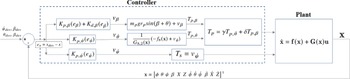

 γTp,θ˙+δTp,β
 βdes
 ∘

 βdes
 ∘

 βdes
 ∘


 β

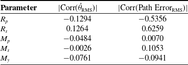

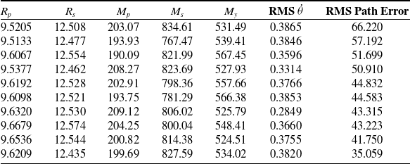
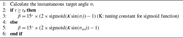


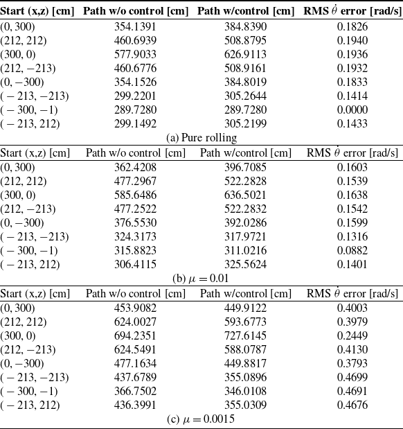
 μ
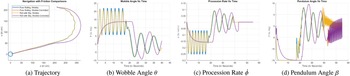
 μ=0.01

 μ=0.003

 μ=0.0015


