1.0 INTRODUCTION
For more than two decades, multi-agent systems have received the attention of various researchers due to their advantages over single-agent systems. In multi-agent applications, one of the issues raised is how to specify the position of members in a group and maintain it with regard to connections between members, which is called formation and is paramount in multi-agent systems. Many works have been carried out regarding formation design, which can be classified into three groups.
A. Virtual structure approach
In this approach, complying with a virtual structure, members of a group maintain a specific formation with respect to each other. Moreover, formation in a virtual structure is considered as a single unit, and each member specifies and preserves a specific formation in this unit(Reference Anthony and Kar-Han1). The position of all members is determined relative to the centre of the virtual structure(Reference Pantelimon, Tepe, Carriveau and Ahmed2). In addition, by minimising the position difference between actual formation and the virtual structure with a kind of controller, actual formation tends toward the virtual structure and is able to track it(Reference Liu and Bucknall3).
B. Behaviour-based approach
This approach is a decentralised approach to control robots(Reference Issa Bayadir and Rashid Abdulmuttalib4), which is inspired by group behaviours of animals(Reference Ai, Yu, Chen, Chen and Shen5). The control law for each member in formation is an optimal combination of rules such as formation keeping, obstacle avoidance and target tracking(Reference Do and Pan6). The main problem with this method is the difficulty in mathematical modeling of the group, which is hard to prove stability of the group and its convergence to formation(Reference Consolini, Morbidi, Prattichizzo and Tosques7). In this approach each agent is controlled by a predefined behaviour(Reference Lee and Chwa8).
C. Leader-follower approach
In this approach, one member is selected as the group leader who is obeyed by the other group members. Orders and information to navigate the group are mostly given to the leader, who, therefore, plays the leading role and is critical to the group. As a result, the entire group faces difficulty in complying with the challenging environment in case of the leader’s failure. To solve this problem, the virtual leader concept is developed.
In practice, the leader-follower approach is more appropriate than other methods due to simple design and scalability(Reference Peng, Wang, Chen, Hu and Lan9). A review of the literatures shows that this method is still widely used despite its single point of failure, and theoretically guarantees formation stability and convergence(Reference Qian, Tong and Li10).
Many tools, such as the direct Lyapunov method, input-output linearisation, backstepping, graph theoretic techniques, the artificial potential field (APF) method, etc., are used in the leader-follower method(Reference Kowdiki, Barai and Bhattacharya11). Among these techniques, the potential function method has been the focus of many researchers due to simple design and feasibility for real-time system control, although it suffers from the local minima problem(Reference Dang, La, Nguyen and Horn12). In 1986, Khatib(Reference Khatib13) presented APFs for obstacle avoidance. Reif and Wang(Reference Reif and Wang14) considered a distributed control approach of autonomous robots. They showed that using APFs with quasi-static modeling can give feasible social behaviours.
In the past few years, some researchers have improved the typical APF method by combining it with other methods(Reference Dong, Hua and Seiichi15). Chen and Yu(Reference Chen, Yu, Su and Luo16) updated the APF method with an additional control force that can be calculated by using the optimal control method. Etemadi et al.(Reference Etemadi, Vatankhah, Alasty, Vossoughi and Boroushakic17) used a Leader Agent that actively motivates flocking at high speed by using local information and a Particle-Swarm-Optimization algorithm. Min et al.(Reference Min, Sun and Niu18) ensured vehicle collision and obstacle avoidance by comprehensively utilising the APF method and the gyroscopic force approach. It also solves the local minima problem existing in the APF method. Etemadi et al.(Reference Etemadi, Alasty and Vossoughi19) analysed the swarm motion as a quasi-static model in static environments based on APFs. They also considered that the visibility of members to each other and to environmental objects would fade due to the increasing distance. Additionally they discussed coordination of a group of agents by a coordinator agent(Reference Etemadi, Alasty and Vossoughi20). In this work, agents had identical finite sensing radii and accessed only local information. It was proved that if a fraction of agents was informed, the centre of mass of the multi-agent system would track the virtual leader. Hengster et al.(Reference Hengster-Movric, Bogdan and Draganjac21) analysed stability properties of a multi-agent control system with an artificial potential based on bell-shaped functions. Gazi et al.(Reference Gazi, Fidan, Hanay and Koksal22) considered formation control as a special form of swarm aggregation, where the final aggregated form of the swarm was desired to constitute a particular predefined geometrical configuration defined by a set of desired inter-agent distance values. Harder and Lauderbaugh(Reference Harder and Lauderbaugh23) specifically addressed formation control, where the objective was to drive a variable number of agents toward a desired parametrically defined shape subject to a stable set of interaction rules and a common navigational objective. Their method was based on APFs.
Many researchers have focused on formation control design using APF approach, but most of them have closed and convex configuration. Because of local minimum phenomena in APFs, the design of open and concave shapes, especially straight-line formation, is difficult and thus has been less investigated. However, the algorithm designed in this work proposes V-shape formation with an adjustable apex angle and also forms a straight-line by increasing the angle to 180°. The number of agents is also variable.
2.0 FORMATION CONTROL DESIGN
In this work, V-shape and straight-line formation are considered as applicable cases of open and concave shape formation. Since this formation is mainly used for surveillance and reconnaissance applications, the parallel motion of unmanned aerial vehicles (UAVs) on a straight-line perpendicular to the trajectory of the leader is our objective.
2.1 Single integrator agent model
Multi-agent systems as imagined here, for path planning, are homogenous, and members are considered to be dimensionless, which are normal assumptions in this field of studies. We also consider no time delay in the motion of swarm members.
The simplest mathematical representation of agents used for studying the behaviour of multi-agent systems is the single integrator model. In this model the motion of an agent i, i = 1… , N is given by
 \begin{equation}{\skew2\dot{p}_i} = {u_i}\end{equation}
Where
 ${p_i} \in {\mathbb{R}^n}$
is the state of agent i and
 ${u_i}$
is the total control input. We assume that all individuals move simultaneously and know the exact relative position of other individuals(Reference Gazi and Passino24).
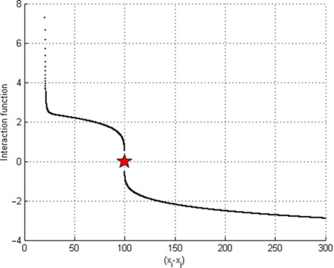
The control input (the interaction function between individual agents) is designed to force agents to reach a predefined position in the formation. For obtaining a useful control input applicable in safe and high-speed mobile robots, we introduce a new inter-agent function between individual agents. We attempt many scenarios and perform ample simulations which result in the following inter-agent function:
 \begin{align}{u_{fi}} = \left\{
\begin{array}{l@{\quad}l}
- \sum \limits_{j=1}^N {w_i}{{\left(\kern1.3pt{{p_{ij}} - {d_{ij}}} \right)}^\beta }{e_{ij}} & {p_{ij}} \ge {d_{ij}}\\
\sum \limits_{j=1}^N {w_i}{{\left( {{d_{ij}} - {p_{ij}}} \right)}^\beta }\left( {{1 \over {{{\left(\kern1.3pt{{p_{ij}} - {d_c}} \right)}^2}}}+1} \right){e_{ij}}&{p_{ij}} < {d_{ij}}
\end{array}\right.\end{align}
 ${u_{fi}}{:}$
The formation control input (the inter-agent function).
 ${W_i}{:}$
Weighting factor.
 ${d_{ij}}{:}$
Desired distance between agents i and j.
 ${p_{ij}} = \|{p_{i - }}{p_j}\|$
Euclidean distance between agents i and j.
 ${e_{ij}}{:}$
unit vector of
 $\left(\kern1.3pt{{p_{i - }}{p_j}} \right)$
.
 $\beta{:}$
Speed smoothness factor (
 $0 < \beta \le 1$
). This factor is introduced for obtaining a uniform variation of inter-agents’ function magnitude. This issue is important in practical applications, such as enchasing sliding mode control on a designed path.
 ${d_c}{:}$
The critical distance between agents, which is equal to the diameter of the private area around every agent. When the distance between two agents reduces to
 ${d_c}$
, the repulsive function tends to infinity (Fig. 1).
The inter-agent function,
 ${\textit{d}_{\textit{c}}=\text{20}}$
,
 ${\textit{d}_{\textit{ij}}}=\text{100}$
and
 $\beta = \text{.2}$
.

2.2 Motion stability analysis
We can define the inter-agent potential function by integrating of Equation (2) from an equilibrium position
 $p_{ij}^* = {d_{ij}}$
to any other relative position
 ${p_{ij}}$
, as follows:
 \begin{equation}U(\kern1.3pt{{p_i}}) =\int_{p_{ij}^{\ast}}^{{p_{ij}}}\, {u_i}\,d{p_{ij}}\end{equation}
For stability analyses, we use the direct Lyapunov method. If we consider the potential function in Equation (3) as a Lyapunov function:
 \begin{equation*} V(\kern1.3pt{{p_i}}) = U\!\left(\kern1.3pt{{p_i}} \right)\end{equation*}
The time derivate of the Lyapunov function is
 \begin{equation*}\skew2\dot{V}(\kern1.3pt{{p_i}}) = {\left[ {{{\Delta }}U\!\left(\kern1.3pt{{p_i}} \right)} \right]^T}{\skew2\dot{p}_i} = - {\skew2\dot{p}_i}^T{\skew2\dot{p}_i} = - {\left\| {{{\skew2\dot{p}}_i}} \right\|^2} \le 0\end{equation*}
As can be observed,
 $V(\kern1.3pt{{p_i}})$
is decreasing for all t unless
 ${\skew2\dot{p}_i}=0$
. Thus the motion dynamic is stable. However, to study global asymptotic stability, we can use the global invariant set theorem stated in Slotine’s study(Reference Slotine and Li25), based on the implicit theorem, because
-
–
 $V(\kern1.3pt{{p_i}}) \to \infty {\rm{\ }}as{\rm{\ }}{\|p_i\|}{\rm{}} \to \infty $
-
–
$\skew2\dot{V}(\kern1.3pt{{p_i}}) \le 0{\rm{\ }}over{\rm{\ }}the{\rm{\ }}whole{\rm{\ }}state{\rm{\ }}space$


If we consider
 $R = \{ {{p_i}{\rm{}}:{\rm{}}\skew2\dot{V}(\kern1.3pt{{p_i}})=0} \} = \{ {{p_i}{\rm{}}:{p_{ij}} = {d_{ij}} = {\rm{}}{p_{ij}}^{*}{\rm{}}} \}$
as the set point of
 $\skew2\dot{V}(\kern1.3pt{{p_i}})=0$
, then
 $M = \{ {{p_i}{\rm{}}:{\rm{}}{{\skew2\dot{p}}_i}=0} \} = \{ {{p_i}{\rm{}}:{p_{ij}} = {d_{ij}} = {\rm{}}{p_{ij}}^{*}{\rm{}}} \}$
is the largest invariant set in R and all solutions globally asymptotically converge to M as
 $t \to \infty $
. Thus base on the global invariant set theorem, we conclude that the group is globally asymptotically stable.
First agent auxiliary force.

2.3 Auxiliary forces
In the application of the potential function method, local minima are highly possible to occur. Therefore, it is extremely difficult to reach an optimal minimum due to occurrences of numerous local minima(Reference Rimon and Koditschek26). All the local minima, except one that is the optimal formation, are at points where attraction and repulsion forces are brought into equilibrium, thereby making it difficult to identify the optimal minimum(Reference Yao, Ordonez and Gazi27).
In this research, we propose a geometric and vectorial method to deal with the problem of local minima. To this end, we define small auxiliary forces and name
 ${u_{ai}}$
where
 $i \in \left[ {1,N} \right]$
. In fact, auxiliary forces are small forces that lead agents toward a predefined position in the formation when the total force applied to agents becomes zero. In other words, they are trapped in an undesirable local minimum.
In this section, All
 ${\bar p_i}\left( {i=1,2, \ldots ,N} \right)$
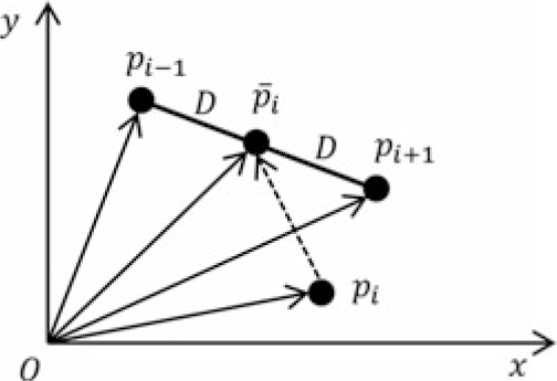
represent assumed desirable positions in the desirable formation, towards which, members that are stuck in an undesirable local minimum, have to be moved. The positions of these assumed points are obtained by the geometric positions of its two adjacent members. Three types of auxiliary forces are introduced here:
End agents’ auxiliary forces:
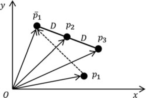
In the V formation structure, two agent have the role of end agent: agent 1 and agent N. For agent 1 the auxiliary force is calculated from Equation (4) as shown in Fig. 2.
 \begin{align}\overrightarrow {{p_3}{p_2}} &= \overrightarrow {o{p_2}} - \overrightarrow {o{p_3}}\nonumber\\[4pt] \overrightarrow {{{\overline {op} }_1}} &= o\overrightarrow {{p_3}} +2\overrightarrow {{p_3}{p_2}}\nonumber\\[4pt] {\vec u_{a1}} &= a( {\overrightarrow {\overline {o{p_1}} } - \overrightarrow {o{p_1}} }) \end{align}
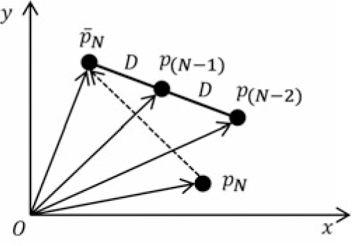
Similarly, for agent N the auxiliary force is calculated from Equation (5) as shown in Fig. 3.
 \begin{align}&\overrightarrow {{p_{\left( {N - 2} \right)}}{p_{\left( {N - 1} \right)}}} = {\overrightarrow{op} _{\left( {N - 1} \right)}} - {\overrightarrow {op} _{\left( {N - 2} \right)}}\nonumber\\[3pt]
&\overrightarrow{\overline{op}_{N}} =\overrightarrow {op}_{(N-2)}+2\vec{p}_{(N-2)}\vec{p}_{(N-1)}\nonumber\\[3pt]
& \vec{u}_{\!aN}=\varepsilon(\overrightarrow{\overline{op}_{N}}-\overrightarrow {op}_{N}) \end{align}
Nth agent auxiliary force.

Middle agent auxiliary force.

Apex (middle) agent auxiliary force:
In the V formation structure the agent
 ${{N+1} \over 2}$
has the role of apex agent. In a special case when apex angle
 $\alpha = \pi $
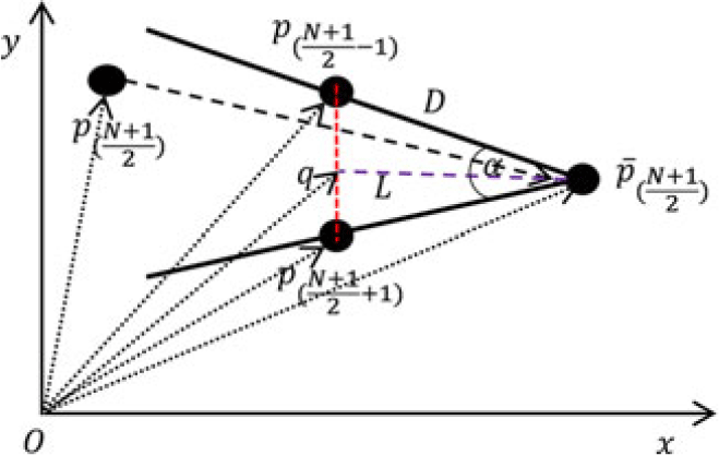
, then there is no apex and this agent has the role of middle agent. For this agent the auxiliary force is calculated from Equation (6) as shown in Fig. 4.
 \begin{equation*}\vec d = {\overrightarrow {op} _{\left( {{{N+1} \over 2} - 1} \right)}} - {\overrightarrow {op} _{\left( {{{N+1} \over 2}+1} \right)}}\end{equation*}
 \begin{equation*}\overrightarrow {ed} = {{\vec d} \over {\left\| {\vec d} \right\|}},\,\overrightarrow {ed} = \left[ \begin{array}{l} {{x_{ed}}} \\[3pt] {{y_{ed}}}\end{array}\right]\end{equation*}
 \begin{equation*}\overrightarrow {el} = \left[ \begin{array}{c} {{\phantom{-}y_{ed}}} \\ { - {x_{ed}}} \end{array} \right],\,\vec L = Dcos\left( {{\alpha \over 2}} \right)\overrightarrow {el} \end{equation*}
 \begin{equation*}\overrightarrow {oq} = {\overrightarrow {op} _{\left( {{{N+1} \over 2}+1} \right)}} + {{\vec d} \over 2}\end{equation*}
 \begin{align}{\overrightarrow {\overline {op} } _{\left( {{{N+1} \over 2}+1} \right)}} &= \overrightarrow {oq} + \vec L \nonumber\\[4pt]
{\vec u_{a\left( {{{N+1} \over 2}} \right)}} &= \varepsilon\!\left( {{{\overrightarrow {\overline {op} } }_{\left( {{{N+1} \over 2}} \right)}} - {{\overrightarrow {op} }_{\left( {{{N+1} \over 2}} \right)}}} \right)\end{align}
Other agents’ auxiliary force:
In the V formation structure for the remaining agents
 $\left( {i \ne 1,N,{{N+1} \over 2}} \right)$
, the auxiliary forces are calculated from Equation (7) as shown in Fig. 5.
 \begin{align} \overrightarrow {{p_{( {\iota+1})}}{p_{( {\iota - 1})}}} &= {\overrightarrow {op} _{\left( {i - 1} \right)}} - {\overrightarrow {op} _{\left( {i+1} \right)}} \nonumber\\ \overrightarrow {\overline {o{p_{\iota}}} } &= {\overrightarrow {op} _{\left( {i+1} \right)}} + {1 \over 2}\overrightarrow {{p_{( {\iota+1})}}{p_{( {\iota - 1})}}} \nonumber\\ {{\vec u}_{ai}} &= \varepsilon \!\left( {\overrightarrow {\overline {o{p_i}} } - \overrightarrow {o{p_i}} } \right) \end{align}
3.0 LEADER TRACKING
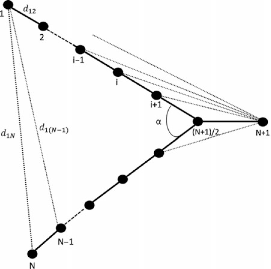
In order to move the group on the desired path while keeping the formation, it is necessary for agents to follow a virtual leader. We assume that the leader is navigated (online or offline) from the ground station. Hence, the main problem in this section is the design of the leader-following algorithm while maintaining the desired formation. For this purpose, we present an algorithm, in which agents and the virtual leader establish a new formation (Fig. 6).
Ith agent auxiliary force
 $\forall \text{i}\left[ {\text{1},\ \textit{N}} \right],\ \textit{i} \ne \text{1},\ \textit{N,}\ \frac{\text{N}+\text{1}}{\text{2}}$
.

Desired position of agents.

The leader is considered as agent N + 1, and the relations between agents, including the leader, are selected the same as the previous section (only with different weighting factor). The leader is supposed to draw the entire group. Hence by moving the leader, the entire group will follow the leader. The entire following agents and the leader form a Y-shape formation as shown in Fig. 6.
Considering the leader agent, for calculating total input control signal it is necessary to include the effect of the leader agent as well. Therefore, for calculating total input in Equation (1) it is necessary to consider the auxiliary force
 ${\vec u_{ai}}$
and the leader-follower inter-agent force
 ${\vec u_{N+1}}$
as follows:
 \begin{equation}{\vec u_i} = {\vec u_{fi}} + {\vec u_{ai}},\quad i=1,2,\ldots ,N+1\end{equation}
It is noted,
 ${\vec u_{ai}}$
is only applied when the agents are trapped in an undesirable local minimum.
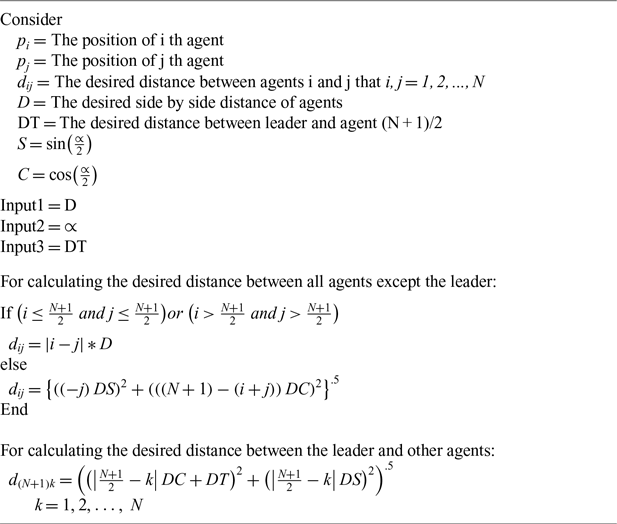
By reflecting on the geometric progression relations and the governed discipline between members of group, we can find a short and useful Algorithm I to obtain a geometric relationship between agents.
This algorithm gives feasible responses for any population of agents. It only requires to tune the weighting factor of inter-agent forces due to changes in the problem scale with increasing number of agents.
Obtaining the desired geometric position of agents

4.0 OBSTACLE AVOIDANCE (OA)
In UAVs formation flight, collision avoidance and obstacle avoidance are key factors and are directly related to flight safety, which has to be considered in detail. In general, OA systems can be divided into two sections: obstacle detection and collision avoidance. This study assumes a predefined obstacle detection mechanism and available obstacle information and only focuses on OA policy design. To design OA systems, various methods have be proposed, which can be classified into four major groups:
A. Predefined collision avoidance
It is a predefined path design to avoid obstacles. An advantage of this method is quick reaction to obstacles. However, it cannot be used when facing unexpected and unpredicted obstacles and in online missions(Reference Albaker and Rahim28). Examples of works in this field are provided in Refs. Reference Bilimoria, Sridhar and Chatterji29 and 30.
B. Geometric approach
This approach uses geometric relations between agents and obstacles to perform calculations and design an OA algorithm. It uses the location, velocity, and heading information of agents and obstacles(Reference Pham, Smolka, Stoller, Phan and Yang31). In Ref. Reference Sasongko, Rawikara and Tampubolon32, an OA algorithm is proposed that locates and designs paths via ellipses that encircle obstacles in the path. Fiorini and Shiller(Reference Fiorini and Shiller33) introduced the concept of obstacle velocity. In their approach, agents have to move at a velocity that is not in the motion range of obstacles to avoid colliding moving obstacles. This was only suitable for obstacles that moved at a constant velocity. Jianhua and Robert(Reference Jianhua and Robert34) improved the relative velocity method to avoid obstacles moving at varying velocities in an unknown dynamic environment. Some other examples are provided in literature(Reference Park, Oh and Tahk35–Reference Phuong, Recchiuto and Sgorbissa37).
C. Optimised trajectory approach
This approach transforms OA into an optimisation problem and solves it by common techniques. In this method, the combination of a kinematic model and a set of constrains typically result in an optimisation problem, that provides the design of a desirable path to avoid obstacles(Reference Albaker and Rahim28). In Refs. Reference Srikanthakumar, Liu and Chen38 and Reference Srikanthakumar and Chen39, the criterion of the distance between a flying robot and an obstacle in terms of the worst performance condition of the flying object transforms into an optimisation problem, which is solved by the Metaheuristic Algorithms.
D. Force field approach
The artificial potential field (APF) approach has been considered by many researchers due to its simple design and suitability for online control. In this approach, the collision avoidance of group members and environmental obstacles may be ensured by defining attraction and repulsion functions and controlling the geometric arrangement. Hence, in this paper we have employed this approach to design a geometric arrangement and OA algorithm.
4.1 OA algorithm
The goal of designing the OA algorithm in this section is to primarily ensure that the members will not collide with obstacles. In the second place in order to avoid collision with obstacles, a UAV has to deviate from its original path. Since imaging is supposed to be the main mission in this paper, the UAV has to pass the obstacle by a minimum acceptable radius in its path. The minimum acceptable radius is equal to the minimum turn radius of the UAV which depends on the velocity as well. This is important because fixed-wing UAVs have non-holonomic constraints and also minimum allowed velocity, which should be considered in designing paths for such UAVs.
As mentioned, a common method to design OA algorithms is the potential function method. It can prevent collision between robots and obstacles by repulsive forces. However, local minimums beside obstacles remain as the weaknesses of this method in designing the path of non-holonomic robots. Thomas et al.(Reference Stastny, Garcia and Keshmiri40) incorporated a morphing factor into the typical potential function, attempting to consider the kinematic constrains of fixed-wing UAVs in OA algorithms.
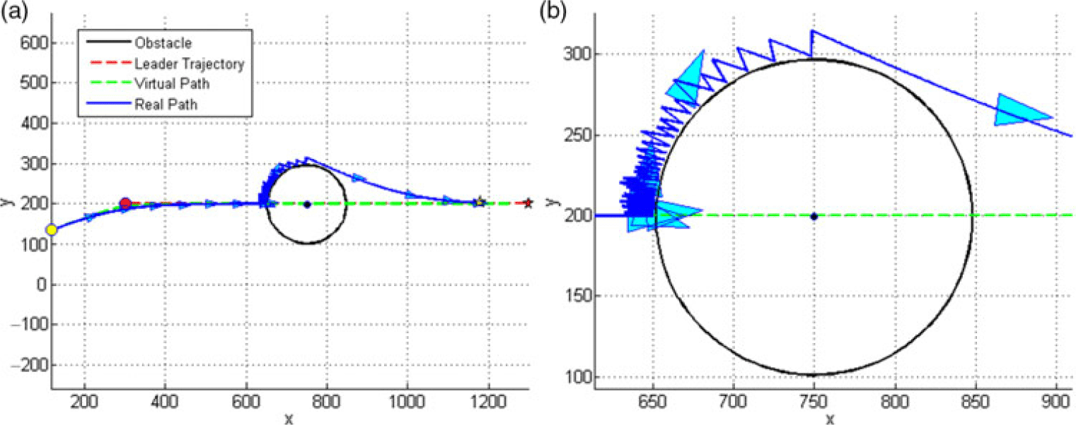
When an agent moves close to an obstacle, if its velocity is directed toward the centre of the obstacle, then the repulsive effect of the obstacle may drastically affect the magnitude and direction of the velocity of the agent. In some cases, the agent’s velocity may vanish or even it may move back from the obstacle. This is not consistent with the performance features of fixed-wing UAVs, and it is not possible to design a path via this practice for the non-holonomic flying vehicles. This will be graphically shown later in Fig. 10. This study attempts to resolve the problem by designing an algorithm named variable repulsive circles (VRCs).
We design two types of paths to design the obstacle avoidance mechanism. The first type includes virtual members’ paths designed based on the forming of the formation algorithm introduced in the previous sections. These members do not sense the obstacles and pass through them. They merely introduce paths that pursue the group leader ideally while forming the appropriate desirable formation. These virtual paths will be the reference for designing the obstacle avoidance mechanism. The second type involves the paths of the real members. These members follow the group leader and maintain the desirable formation as much as possible, meanwhile perceiving the obstacles and observing the defined principles of obstacle avoidance. The rules set for guiding real members would vary from those for virtual members. In this part, each real member is directed toward its corresponding virtual member by the following potential function by a decentralised approach independent from other members.
 \begin{equation*}{U_{fri}} = {1 \over 2}{w_{ri} }{\left(\kern1.3pt{{p_{ri} }- {p_i } }\right)^2 }\end{equation*}
Where,
 ${U_{fri}}$
is the real agent formation control potential function,
 ${w_{ri}}$
is weighting factor,
 ${p_i}$
and
 ${p_{ri}}$
are virtual and real agents’ positions, respectively.
The same repulsive force introduced in Equation (2) is used to guarantee the non-collision of real members with each other, which will be activated whenever the distance between two real members reduced to less than the distance defined in the desirable formation.
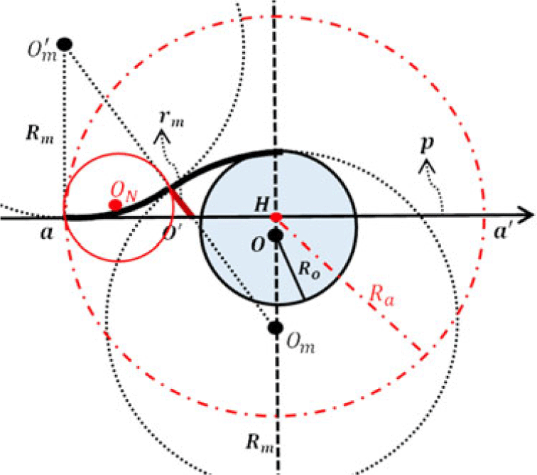
We assume an imaginary circle in the two-dimensional space (a sphere in the three-dimensional space) around the obstacle and name it Repulsive Circle. The repulsive circle is activated and repels agents immediately when the agents collide with it. In the next step, we draw a curve parallel to the leader movement path curve such that it passes through the centre of the obstacle and name it virtual path. As shown in Fig. 7, we draw circles with the radius of
 ${R_m}$
(the minimum turn radius of UAVs) such that the first circle is tangent to the repulsive circle and encircles it. The centre of this circle lies on a line, that is normal to the virtual path and passes through the centre of the obstacle. The second circle is tangent to both the virtual path and the first circle. One segment of each circle is used to design a smooth path which is shown in Fig. 7. This path can direct UAVs around obstacles in a way that obstacle avoidance happens with no sudden change of direction.
OA mechanism.

Thus, in the worst collision case where a UAV directly heads toward the obstacle’s centre, the maximum deviation of the path will be the minimum turn radius of UAVs. Thereby, the UAVs can follow the designed path.
Now we assume variable repulsive circles centered on the virtual path. The repulsive circle’s radii begin from zero at point
a
(the location where the UAV turn circle is tangent to the virtual path) and continue to grow to
 ${{\rm{R}}_o}$
at point
O
(the obstacle’s centre) as shown. In the following, the radii continue to reduce to zero at
 $\textbf{\textit{a}}^{\prime}$
. These circles will continue to grow as the agent moves closer to the obstacle.
Other data of the designed OA mechanism in Fig. 7 is as follows:
 ${\rm{p}}(i)$
: Virtual path.
 ${\textbf{\textit{R}}_{\textbf{\textit{m}}}}$
: Minimum turning radius of UAVs.
 ${\textbf{\textit{R}}}_{\textbf{\textit{o}}}$
: Radius of obstacle.
 $\textbf{\textit{O}}$
: Centre of obstacle.
 ${\textbf{\textit{O}}_{\textbf{\textit{m}}}}\textbf{(\textit{i})}\ \textrm{and}\ \textbf{\textit{O}}_{\textbf{\textit{m}}}^{\prime}(i)$
: Centres of minimum turn circles.
 $\textbf{\textit{a}}\textbf{(\textit{i})}$
: The initial point that repulsive circles begin to grow.
 $\textbf{\textit{a}}^{\prime}\textbf{(\textit{i})}$
: The final point that repulsive circles stop to grow.
 $\textbf{\textit{a}}^{\prime\prime}\textbf{(\textit{i})}$
: The tangent point of two circles
 ${\textbf{\textit{O}}_{\textbf{\textit{m}}}}\textbf{(\textit{i})}\ \textit{and}\ \textbf{\textit{O}}_{\textbf{\textit{m}}}^{\prime}\textbf{(\textit{i})}$
.
 ${\textbf{\textit{r}}_{\textbf{\textit{o}}}}\textbf{(\textit{i})}$
: The variable radius of Repulsive Circle.
 $\textbf{\textit{O}}^{\prime}\textbf{(\textit{i})}$
: The position of VRCs centres.
 ${\textbf{\textit{R}}_{\textbf{\textit{a}}}}\textbf{(\textit{i})}$
: Radius of activation circle. Activation circle acts as a switch, which activates the OA algorithm when any UAV enters inside it.
 $\overrightarrow{\textbf{\textit{OO}}} _{\textbf{\textit{m}}}\textbf{(\textit{i})}$
: The position of the centre of the minimum turn circle that encircles the obstacle.
 $\textbf{\textit{r}}_{\textbf{\textit{m}}}\textbf{(\textit{i})}$
: The amount of
 ${\textbf{\textit{r}}_{\textbf{\textit{o}}}}$
at the tangent point of two minimum turn circles.
 $\textbf{\textit{m}}\textbf{(\textit{i})}$
: The distance of
 ${r_m}$
to O
Which
 ${R_m}$
can be calculated as follows(Reference Anderson41):
 \begin{equation*}{R_m} = {{{v_{min}}^2} \over {g{\rm{tan}}\!\left( {{\varphi _{max}}} \right)}} = {{{v_{min}}^2} \over {g\sqrt {{n_{max}}^2 - 1} }}\end{equation*}
 ${\textbf{\textit{v}}_{\textbf{\textit{min}}}}$
: Minimum speed of UAVs
 $\textbf{\textit{n}}_{\textbf{\textit{max}}}$
: Maximum load factor
 ${\boldsymbol{\varphi}_{\textbf{\textit{max}}}}$
: Maximum bank angle
 ${\textit{R}}_{{\textit{a}}}\textbf{(\textit{i})}$
and
 ${\textbf{\textit{r}}_{\textbf{\textit{m}}}}\textbf{(\textit{i})}$
are computed as follows:
 \begin{align*}{R_a}\textbf{(\textit{i})}{\rm{}} &= \sqrt {4R_m^2 - {{\left( {2{R_m} - {R_o}} \right)}^2}}\\[5pt]
{r_m}\textbf{(\textit{i})}{\rm{}} &= \left( {{{2R_m^2} \over {2{R_m} - {R_o}}}} \right) - {R_m}\\[5pt]
m\textbf{(\textit{i})}{\rm{}}& = \sqrt {{{\left( {{R_m} - {r_m}{(\textit{i})}}\right)}^2} - {{\left( {{R_m} - {R_o}} \right)}^2}}\end{align*}
The main problem here is finding the variation of radii of repulsive circles in which their variation forms a smooth path around the obstacle. To achieve this, first, we find the position of minimum turn circle centre (Fig. 7).
 \begin{align*}\overrightarrow {O^{\prime}O}\textbf{(\textit{i})}{\rm{}} & = \vec O - \overrightarrow {O^{\prime} }\textbf{(\textit{i})}\\[5pt]
{\vec e_{o^{\prime}o}}\textbf{(\textit{i})}{\rm{}} & = {{\overrightarrow {O^{\prime}O} \textbf{(\textit{i})}{\rm{}}} \over {\|\overrightarrow {O^{\prime}O} \textbf{(\textit{i})}{\rm{}}\|}}\\[5pt]
\vec e_{o{o_m}}\textbf{(\textit{i})} & = \left[ \begin{array}{l} {{\phantom{-}{\vec e}_{o^{\prime}o}}\left( {i,2} \right)} \\[3pt] { - {{\vec e}_{o^{\prime}o}}\left( {i,1} \right)} \end{array} \right]\\[5pt]
{\overrightarrow {OO} _m}\textbf{(\textit{i})}{\rm{}} & = \left( {{R_m} - {R_o}} \right){\vec e_{o{o_m}}}\textbf{(\textit{i})}\end{align*}
Then by presented Algorithm II variations of
 ${\textbf{\textit{r}}_{\textbf{\textit{o}}}}$
and consequently the repulsive force can be obtained. Also, Algorithm II defines a rotational force to prevent UAVs from being stuck in local minimums due to a zero resultant of forces in the obstacle collision location.
Figure 7 presents another circle (with centre
 ${O_N}$
and radius
 ${{a^{\prime\prime}} \over 2}$
) known as the navigation circle, which is used to specify the movement direction of the UAV at collision with the spindle shape (a shape created by the segments of the circles of the minimum radius turn around the obstacle). This circle activates a force, which is activated when the UAV enters the circle and conducts the UAV to the circumference of the circle
 ${O^{\prime}}_m$
. The force can be defined as follows.
 \begin{equation}{u_{Ni}} = \left\{ \! \begin{array}{cc}{-} {w_{Ni}}\left(\kern1.3pt{{p_{ri}} - {{O}^{\prime}_m}(i)} \right) & {if\left\| {{p_{ri}} - {O_N}(i)} \right\| \le {{a^{\prime\prime}(i)} \over 2}\,and\,\left\| {{p_{ri}} - {{O^{\prime}}_m}(i)} \right\| \ge {R_m}} \\ 0 & {else} \end{array} \right.\end{equation}
Where
 ${u_{Ni}}$
,
 ${w_{Ni}}$
are navigation force and weighting factor, respectively.
Obtaining the OA and rotation forces

5.0 FINAL ALGORITHM
The final algorithm is a combination of the algorithms introduced in the formation control and OA sections. By adding all control inputs, the model of final group movement can be summarised as:
 \begin{equation}{\skew2\dot{p}_{ri}} = {u_{fri}} + {u_{ci}} + {u_{ai}} + {u_{oi}} + {u_{ri}} + {u_{Ni}},\qquad i=1,2,\ldots ,N\end{equation}
Where
 ${u_{fri}}$
,
 ${u_{ci}}$
,
 ${u_{ai}}$
,
 ${u_{oi}}$
,
 ${u_{ri}}$
,
 ${u_{Ni}}$
are the real formation control input, anti-collision force, axillary force, OA force, rotational force and navigation force, respectively.
6.0 SIMULATION RESULTS
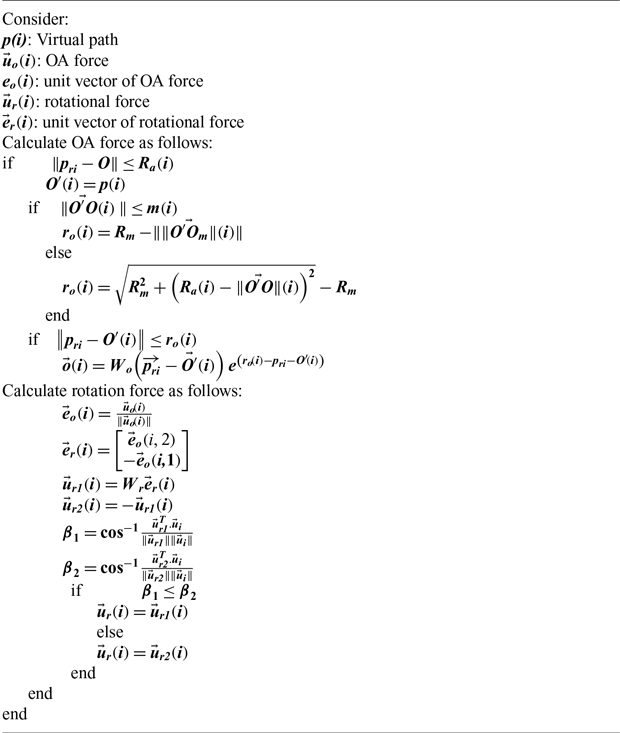
In this section, the simulation results will be presented in the Matlab Software. The performance constraints of RQ-7B, which is a UAV developed by AAI Corporation (headquarters in the United States), are considered in the simulation process. The leader is assumed to move as follows
 \begin{align} {{\skew2\dot{x}}_l} &= {v_l}\,{\rm{cos}}( {{\psi _l}}) \nonumber\\[3pt] {{\skew2\dot{y}}_l} &= {v_l}\sin ( {{\psi _l}}) \nonumber \\[3pt] {{\skew2\dot{\psi} }_l} &= {w_l} \end{align}
Where
 ${p_l}(t) = \left[ {{x_l}(t),{y_l}(t)} \right]$
denotes the position of leader,
 ${\psi _l}$
is heading angle in two-dimensional plane,
 ${v_l}$
is linear speed, and inputs are assumed as:
 \begin{align} {v_l}(t)&=34 \nonumber\\[3pt] {w_l}(t)&=0.05\sin \left( {0.1t} \right) \end{align}
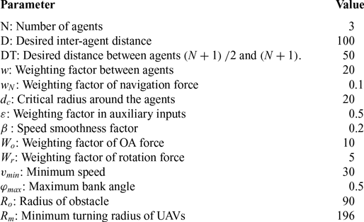
The simulation parameters of the leader tracking algorithm are presented in Table 1. The agent positions are initialised randomly in a rectangle of 500 × 500 with random orientations. In all figures, initial and final positions of agents are marked as yellow circles and yellow stars, respectively.
The simulation parameters

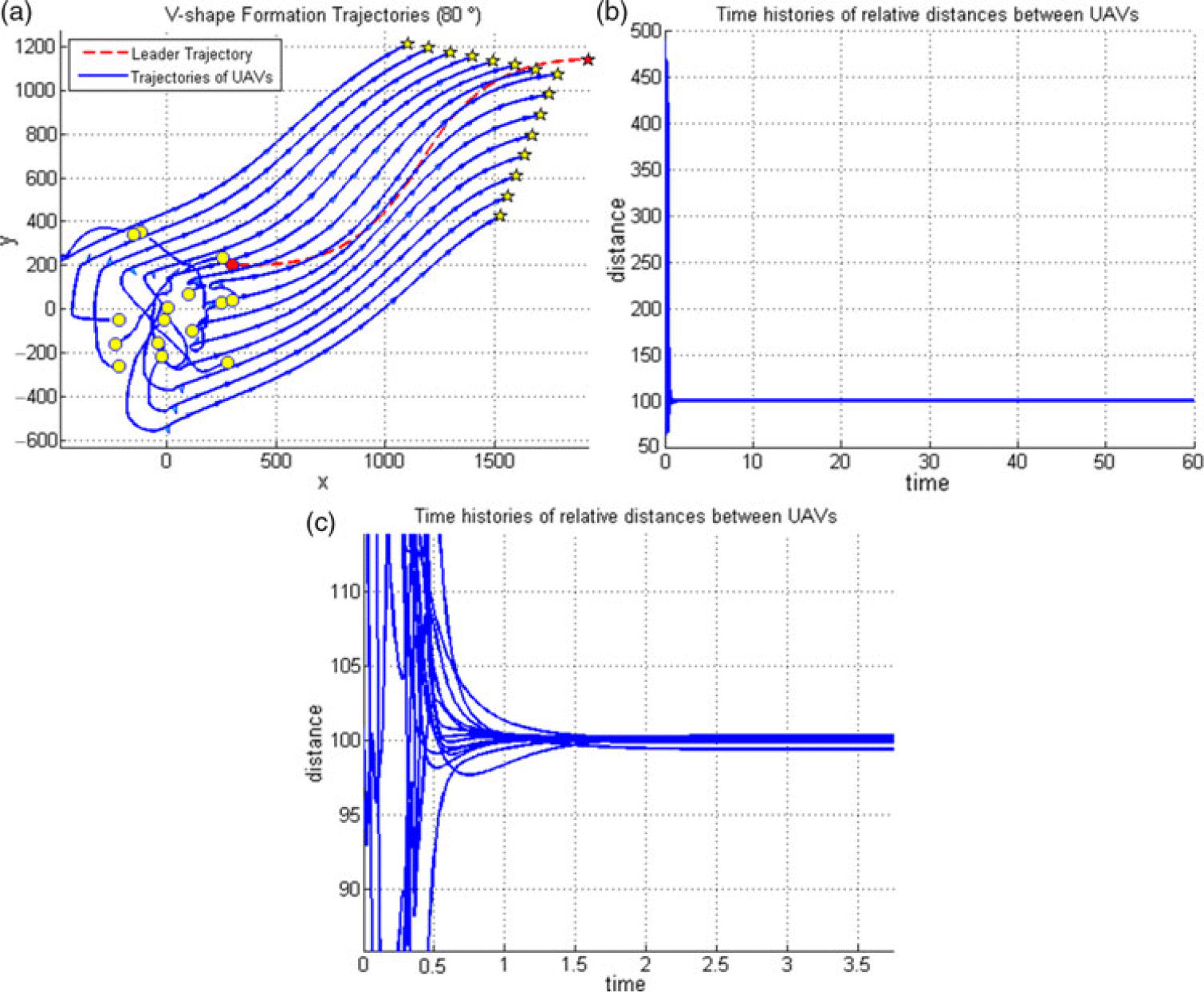
Trajectories of 15 agents with angle of
 ${\text{80}^\circ }$
(a), History of inter-agents distances (b), Zoom of history of inter-agents distances (c).

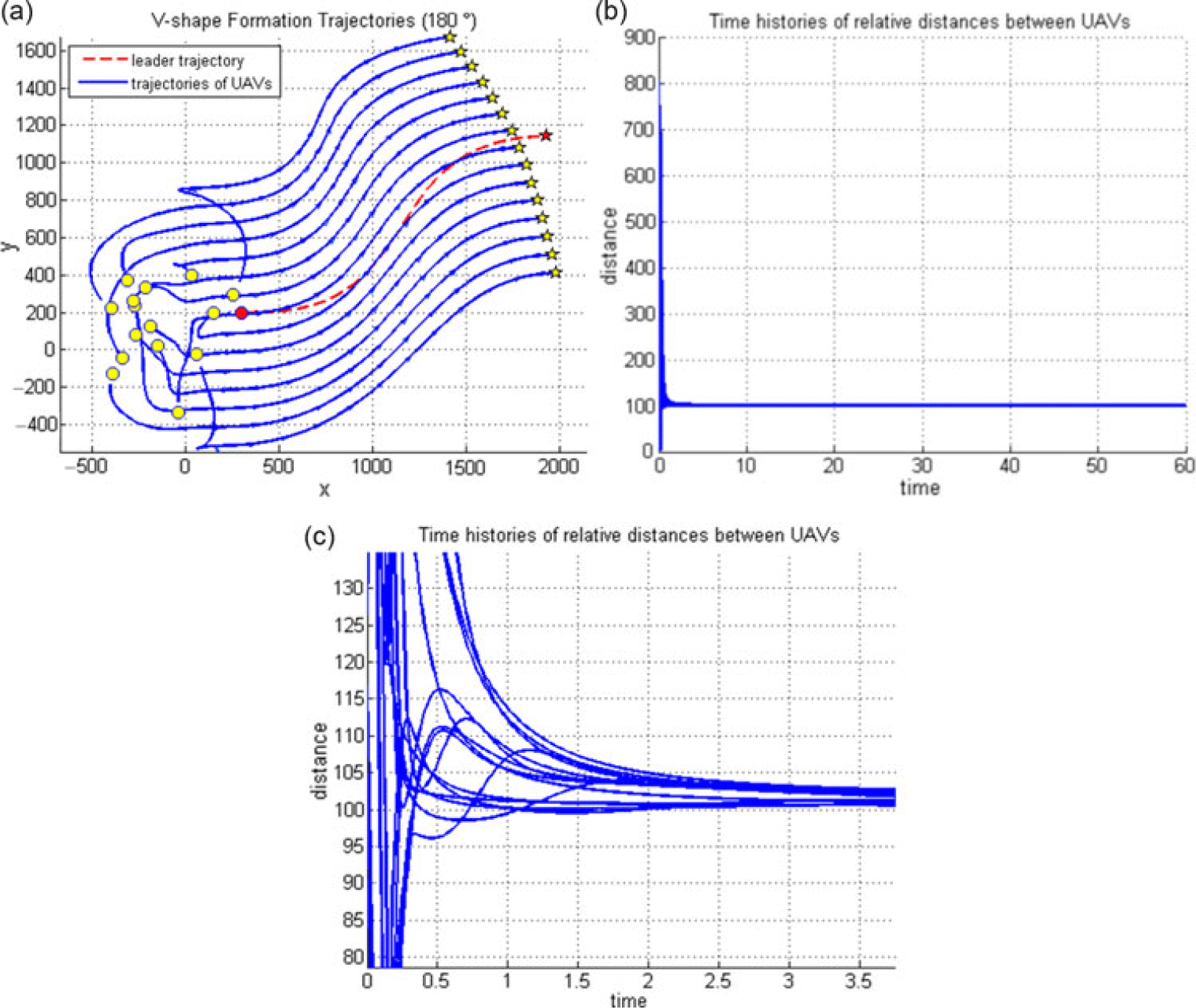
Trajectories of 15 agents with angle of
 ${180^\circ }$
(a), History of inter-agents distances (b), Zoom of history of inter-agents distances (c).

Traditional method.

Colliding with the lateral points outside the centre of obstacle by the introduced method.

Colliding with the middle of the obstacle by the introduced method.

As the impact velocity increases to 42m/s.

Figure 8 illustrate trajectories of V-shape formations of 15 agents with
 ${80^\circ }$
angle. Figure 9 shows the results of the simulation for 15 agents tracking leader with the formation of
 ${180^\circ }$
or straight-line formation. As illustrated, the UAVs not only track the leader but also keep their formation and distance with respect to the virtual leader.
In Figs. 8(c) and 9(c), the diagram of the distance between UAVs (initial moments) shows that trajectories of all UAVs converge to the predetermined distance with each other and leader, while the collision is avoided.
As shown in simulation scenarios, the algorithm has no limitation in selecting the number of members and the V-shaped apex angle in the formation.
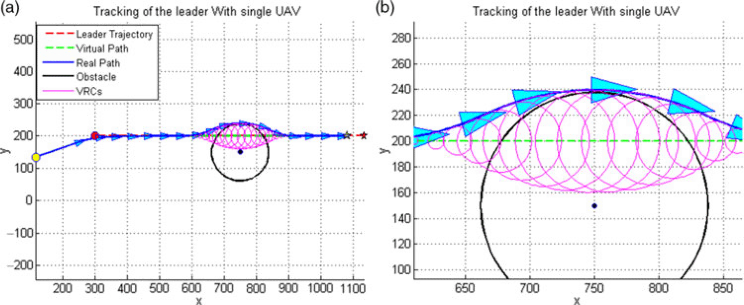
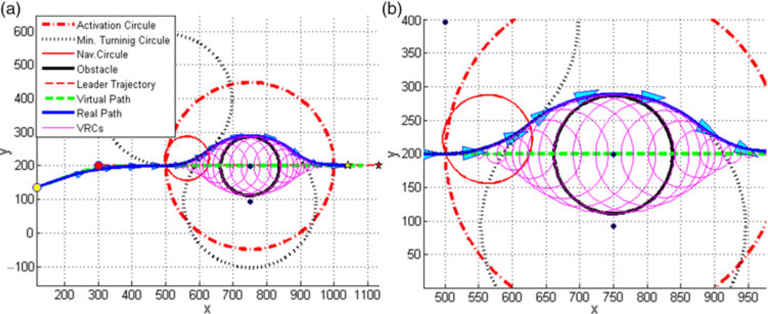
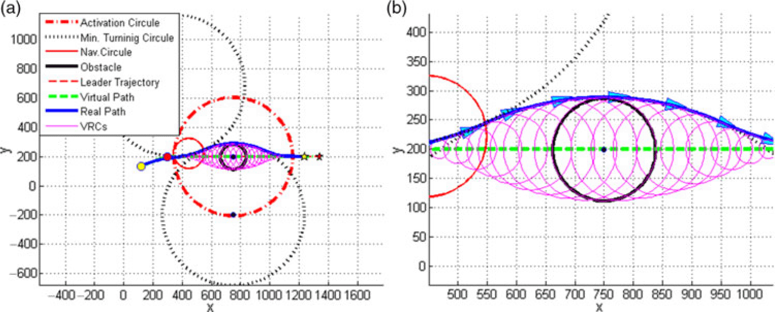
Figures 10, 11, 12 and 13 illustrate the direct trajectory of a UAV in facing an obstacle from different angles. Based on the initial assumption of the problem, considering the obstacle within a circle, only two cases may happen with the collision of the UAV from any angle and direction. In the first case, the collision may occur from lateral points outside the centre of the circle. In such a case, the path deviation rate depends on the distance of the collision point from the centre of the circle (Fig. 11). The second case involves colliding with the middle of the obstacle, which would be the worst possible situation as the highest deviation in the UAV trajectory can occur (Fig. 12).
Encountering an obstacle by the traditional method.

Colliding with the middle of the obstacle by the introduced method.

Colliding with the lateral points outside the centre of obstacle by the introduced method.

Figure 10 shows an image of an agent that faces an obstacle by a traditional method. As seen, instantaneous changes occur in the direction and size of motion at the collision sites. Thus, following these created paths seems to be impossible at all as a result of the structural and functional constraints of fixed-wing UAVs. However, as depicted in Fig. 11, the obtained path experiences slight changes and corresponds to the minimum radius turn circles by using the algorithm introduced. Therefore, the resulting trajectory appears to be compatible with the functional capability of the fixed-wing UAVs.
The UAV colliding the centre of the circle at different speeds is shown in Figs. 12 and 13. As illustrated in Fig. 13, as the impact velocity increases to 42m/s, the radius of the turning circle also enhances to 487m. Consequently, the UAV will turn around the obstacle at a larger radius as well.
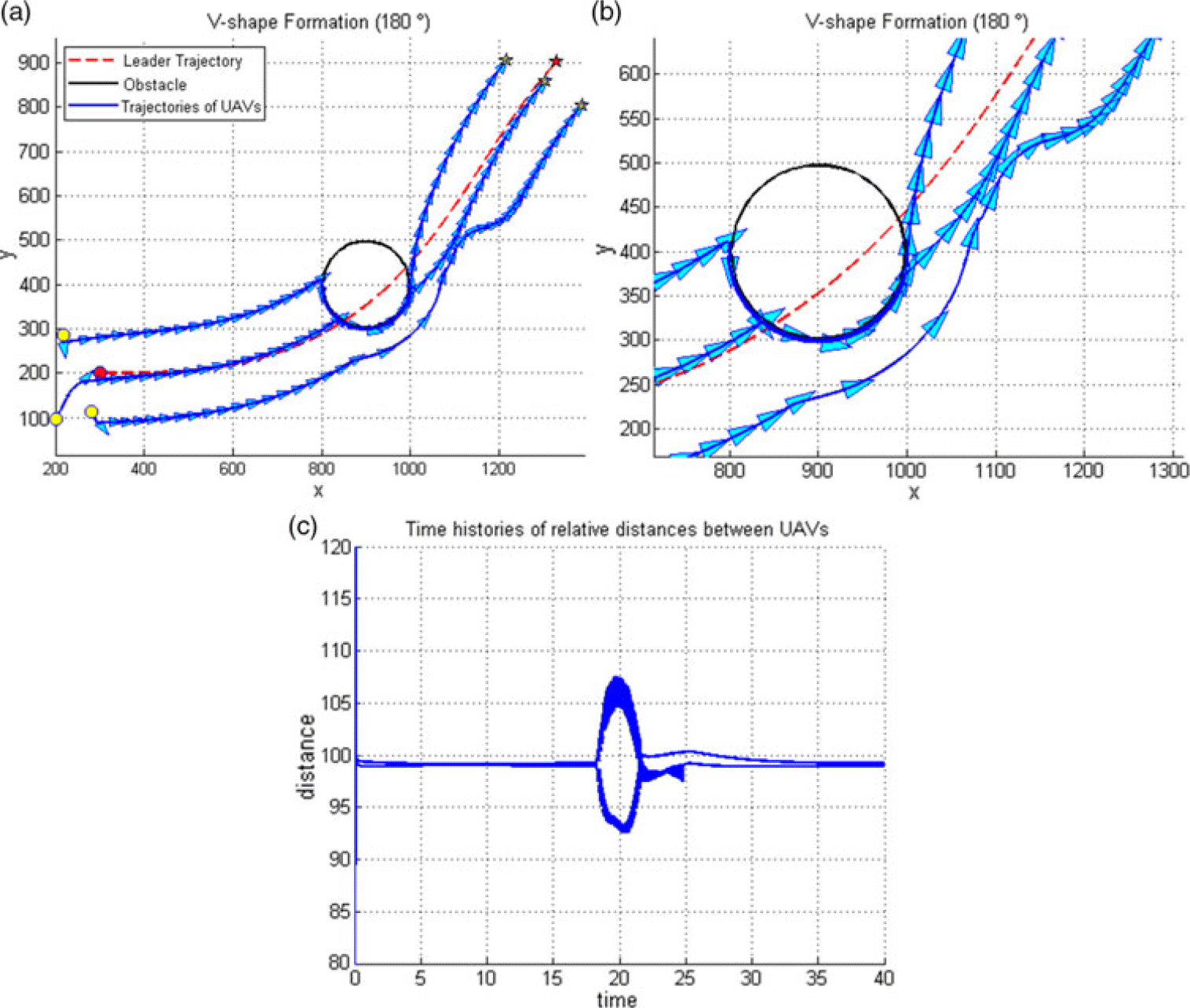
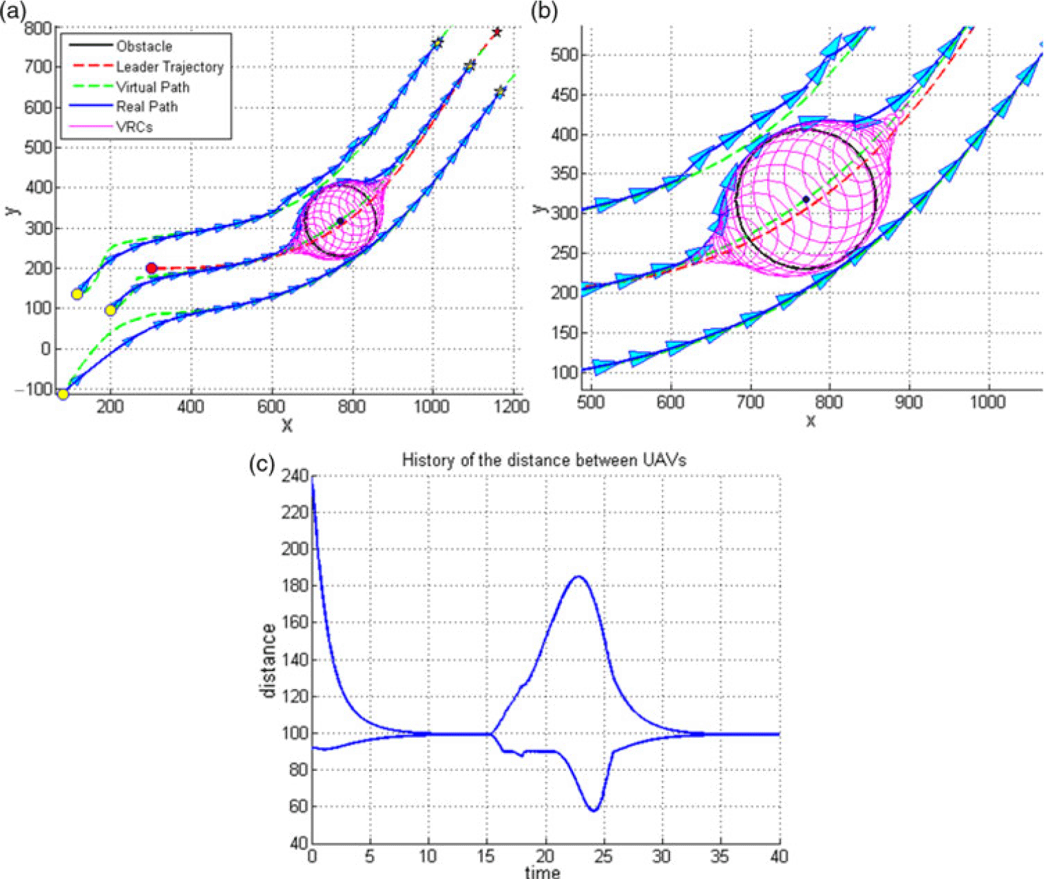
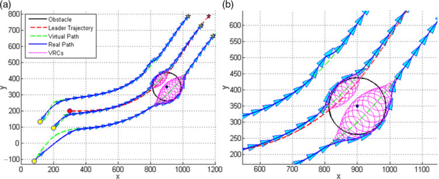
Figures 14, 15 and 16 show the trajectories of three UAVs with V-shaped formation at a 180° angle. At this stage, the collision of the UAVs with the obstacle while turning has been studied to assess the efficiency of the introduced algorithm. Figure 14 presents the formation movement while encountering an obstacle by the traditional method. As evident, instant changes have occurred in the direction of the UVAs, and thereby, the formation structure is fully disorganised. Hence, the path obtained is not consistent with the operating conditions of a fixed-wing UAV. However, applying the designed algorithm (Figs. 15 and 16) has both prevented instant changes in the motion direction and reduced the deformation of the formation as well. Also, given the adaptation of the obtained paths to the minimum radius turn circles, one can say the fixed-wing UAVs can easily pass through these trajectories.
For illustrating different colliding angles while turning in the formation flight, Figs. 15 and 16 presented for cases of colliding with the centre and out of the centre of an obstacle, respectively.
Figures 14c and 15c show the time history of the distance between the UAVs. As can be concluded from the diagrams, the distances between the group members have not become less than the critical distance under no circumstances because of using repulsion potential functions unbounded from left.
The scenarios investigated are indeed the most complex and difficult possible states that may occur in the face of obstacles, especially when the UAVs themselves are turning. Accordingly, other possible situations of collision will obviously be tolerated easily.
7.0 CONCLUSION
Provided that the local minimum problem is eliminated, this study shows that the potential function is an effective method in the formation control even for open and concave formations. The selection and design of a potential function appropriate for the mission, plays an essential role in the accuracy and performance of the formation control system. The simulation results suggest that the proposed repulsive function not only prevented any collision between the components but also prevented the distances between components from reducing below the critical level.
The important features of the proposed algorithm are:
-
1. The algorithm has no limitation in selecting the number of members and the V-shaped apex angle in the formation.
-
2. Due to the use of general terms in mathematical relations, the proposed algorithm is simple and short and does not require considerable coding. Thus, it is suitable for formation control and leader pursuit problems.
-
3. The performance constraints of fixed-wing UAVs are considered in the proposed algorithm’s design.
-
4. The path designed to cross the obstacle is optimal due to the use of the minimum turn radius of UAVs in designing the flight path. Thus, the path obtained is the closest distance from an obstacle that a fixed-wing UAV may pass through without collision. As a result, the least deformation and disorganisation has occurred in the formation.