

1 Introduction
The phase speed of a linear gravity–capillary wave on deep water has its minimum  $c_{min}=23~\text{cm}~\text{s}^{-1}$ at a finite wavelength
 $\unicode[STIX]{x1D706}_{min}=1.71$ cm (Rayleigh Reference Rayleigh1883). There have been many theoretical and numerical studies on forcing-free inviscid two-dimensional (2-D) and three-dimensional (3-D) gravity–capillary waves on deep water with propagation speeds near
 $c_{min}$, mainly concentrating on gravity–capillary solitary waves whose propagation speeds are below
 $c_{min}$ (Vanden-Broeck & Dias Reference Vanden-Broeck and Dias1992; Calvo & Akylas Reference Calvo and Akylas2002; Parau et al. Reference Parau, Vanden-broeck and Cooker2005; Akers & Milewski Reference Akers and Milewski2008, Reference Akers and Milewski2009, Reference Akers and Milewski2010; Milewski et al. Reference Milewski, Vanden-broeck and Wang2010; Kim Reference Kim2012; Wang & Vanden-Broeck Reference Wang and Vanden-Broeck2015).
For the observation or realization of these theoretical gravity–capillary waves on deep water, some experimental studies were recently carried out using a moving 3-D air-blowing forcing (Diorio et al. Reference Diorio, Cho, Duncan and Akylas2009, Reference Diorio, Cho, Duncan and Akylas2011; Masnadi & Duncan Reference Masnadi and Duncan2017a,Reference Masnadi and Duncanb), a moving 3-D air-suction forcing (Park & Cho Reference Park and Cho2016) and a moving 2-D air-blowing forcing (Park & Cho Reference Park and Cho2018). In the experiments of Diorio et al. (Reference Diorio, Cho, Duncan and Akylas2009) and Diorio et al. (Reference Diorio, Cho, Duncan and Akylas2011), 3-D gravity–capillary waves were generated by blowing compressed air through a 3-D nozzle hole that moves (from zero speed) horizontally over the surface of deep water (initially still water) with final constant speeds close to  $c_{min}$, i.e. by using a moving 3-D air-blowing forcing. Four different states were observed according to the forcing speeds (
 $U$). At relatively low speeds below a certain critical speed (
 $U<U_{crit}$), a steady small-amplitude linear circular depression is observed just below the moving air-blowing forcing (state I). As the forcing speed further increases close to
 $c_{min}$ (
 $U_{crit}<U<c_{min}$), steady nonlinear 3-D gravity–capillary solitary waves are observed ‘behind’ the moving forcing (state II). When the forcing speed is very close to
 $c_{min}$ (
 $U\approx c_{min}$), periodic shedding phenomena of 3-D localized depressions are observed obliquely behind the moving forcing (state III); the third regime (
 $U\approx c_{min}$) means that the forcing speed can be either slightly subcritical (
 $U\leqslant c_{min}$) or critical (
 $U=c_{min}$) or be slightly supercritical (
 $U\geqslant c_{min}$), i.e. all are possible. Finally, when the forcing speed is above
 $c_{min}$ (
 $U>c_{min}$), steady ‘V’-shaped depressed waves are observed behind the moving forcing (state IV). All these experimental observations were compared with numerical results based on a model equation (Cho et al. Reference Cho, Diorio, Akylas and Duncan2011). They agree with each other very well. Recently, these experimental works were extended to further investigations of oblique shedding phenomena of 3-D gravity–capillary solitary waves (Masnadi & Duncan Reference Masnadi and Duncan2017a) and the interaction of 3-D gravity–capillary solitary waves (Masnadi & Duncan Reference Masnadi and Duncan2017b). Here, the denotations ‘state I’, ‘state II’ and ‘state III’ were used in Diorio et al. (Reference Diorio, Cho, Duncan and Akylas2009) and Diorio et al. (Reference Diorio, Cho, Duncan and Akylas2011). State I is steady and linear, state II is steady and nonlinear and state III is periodic and nonlinear. They are all localized states. Also, in the present paper, we refer to the last state (steady, linear and non-local waves when
 $U>c_{min}$) as ‘state IV’. Furthermore, henceforth, these terms ‘states I, II, III and IV’ will also be used for gravity–capillary waves generated by 2-D air-blowing, 2-D air-suction and 3-D air-suction forcings if the overall resultant wave states can be similarly categorized according to being steady/periodic/linear/nonlinear as those generated by 3-D air-blowing forcings.
In the experiment of Park & Cho (Reference Park and Cho2016), 3-D gravity–capillary waves were generated by sucking air through a 3-D nozzle hole that moves (from zero speed) horizontally over the surface of deep water (initially still water) with final constant speeds close to  $c_{min}$, i.e. by using a moving 3-D air-suction forcing instead of a moving 3-D air-blowing forcing. As in the case of the 3-D air-blowing forcing, four different states were observed according to forcing speeds (
 $U$). At relatively low speeds below a certain critical speed (
 $U<U_{crit}$), a steady small-amplitude linear circular depression is observed ‘ahead’ of the moving forcing (state I). As the forcing speed further increases close to
 $c_{min}$ (
 $U_{crit}<U<c_{min}$), steady nonlinear 3-D gravity–capillary solitary waves are observed ahead of the moving forcing (state II). When the forcing speed is very close to
 $c_{min}$ (
 $U\approx c_{min}$), oblique shedding phenomena of 3-D localized depressions are observed ahead of the moving forcing. Sometimes, at the end of one shedding sequence, the thread of the water column above the water hump suddenly snaps and the hump collapses instantaneously. Then, after a short time, the hump sticks to the air-suction hole again. Once this happens, these ‘snap-stick’ phenomena are repeated (state III). Finally, when the forcing speed is above
 $c_{min}$ (
 $U>c_{min}$), steady ‘V’-shaped depressed waves are observed ahead of the moving forcing (state IV). All the linear and nonlinear states generated by the 3-D air-suction forcing correspond to those generated by the 3-D air-blowing forcing. The main difference is that waves in states II, III and IV generated by the 3-D air-suction forcing are observed ahead of the forcing, while those generated by the 3-D air-suction forcing are observed behind the forcing.
In the experiment of Park & Cho (Reference Park and Cho2018), 2-D gravity–capillary waves were generated by blowing compressed air through a 2-D narrow slit that moves (from zero speed) horizontally over the surface of deep water (initially still water) with final constant speeds close to  $c_{min}$, i.e. by using a moving 2-D air-blowing forcing. As in the cases of the 3-D air-blowing/air-suction forcing, four different states were observed according to forcing speeds. At relatively low speeds below a certain critical speed (
 $U<U_{crit}$), a steady small-amplitude linear depression is observed just below the moving forcing (state I). As the forcing speed further increases close to
 $c_{min}$ (
 $U_{crit}<U<c_{min}$), steady nonlinear 2-D gravity–capillary solitary waves are observed behind the moving forcing (state II). When the forcing speed is very close to
 $c_{min}$ (
 $U\approx c_{min}$), periodic shedding of 2-D localized depressions is observed behind the moving forcing (state III). Finally, when the forcing speed is above
 $c_{min}$ (
 $U>c_{min}$), a pair of short and long linear waves is observed, respectively, ahead of and behind the moving forcing (state IV). All these experimental observations were compared with numerical results based on a model equation and showed good agreement.
In summary, in the above existing experimental works (and theoretical works as well), for an initial still-water condition, a 2-D/3-D forcing moves from zero speed towards a certain target constant speed ( $U$). In terms of resultant wave states, there exists a certain critical speed (
 $U_{crit}$) below which steady small-amplitude linear 2-D/3-D localized waves are observed (state I,
 $U<U_{crit}$) and just above which steady finite-amplitude nonlinear 2-D/3-D gravity–capillary solitary waves are observed (state II,
 $U_{crit}<U<c_{min}$) and above which periodic shedding phenomena of nonlinear 2-D/3-D localized depressions (state III,
 $U\approx c_{min}$) and steady linear 2-D/3-D non-local waves (state IV,
 $U>c_{min}$) are observed. In particular, the abrupt jump transition from a linear state I to a nonlinear state II is typical for a nonlinear system that may show the so-called hysteresis phenomena, showing the dependence of a state on its history starting from an initial condition. One natural question then arises: Instead of the still-water initial condition, if the initial condition were a state II (or state III or state IV) and the forcing speed were to decrease below the critical speed (
 $U_{crit}$), what will be the final state? A small-amplitude linear 2-D/3-D localized wave (state I) as before or a new steady finite-amplitude nonlinear 2-D/3-D gravity–capillary solitary wave that cannot be observed in the case of increasing the forcing speed? To the best of the present authors’ knowledge, the answer to this question is not known and this is therefore the subject of the present paper. In the next section (§ 2), the experimental set-up will be briefly described. In § 3, experimental results from four different experiments using a moving 2-D/3-D air-blowing/air-suction forcing will be described. In each experiment, from the zero state, by increasing the forcing speed above a critical speed, states II, III and IV will be generated; as will be shown, for the 2-D air-suction case only, in state II, nonlinear finite-amplitude depression waves are generated but are not gravity–capillary solitary waves. Then, with these waves in states II, III and IV as initial conditions, the forcing speed will be decreased below the critical speed (
 $U_{crit}$) to determine whether the final states will be linear small-amplitude 2-D/3-D waves or finite-amplitude nonlinear 2-D/3-D gravity–capillary solitary waves (or 2-D steady localized depressions for a 2-D air-suction case). In § 4, for 2-D/3-D air-blowing cases, in particular, comparisons with simulation results based on a model equation (Cho et al. Reference Cho, Diorio, Akylas and Duncan2011) will be made.
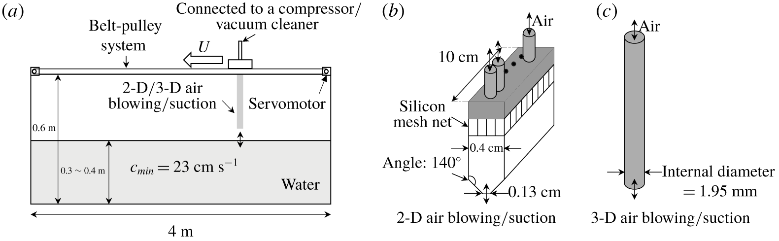
Experimental set-up for 2-D/3-D air-blowing/air-suction tests. (a) Side view of the water tank. (b) A 2-D air-blowing/suction slit. (c) A 3-D air-blowing/suction nozzle.

2 Experimental set-up
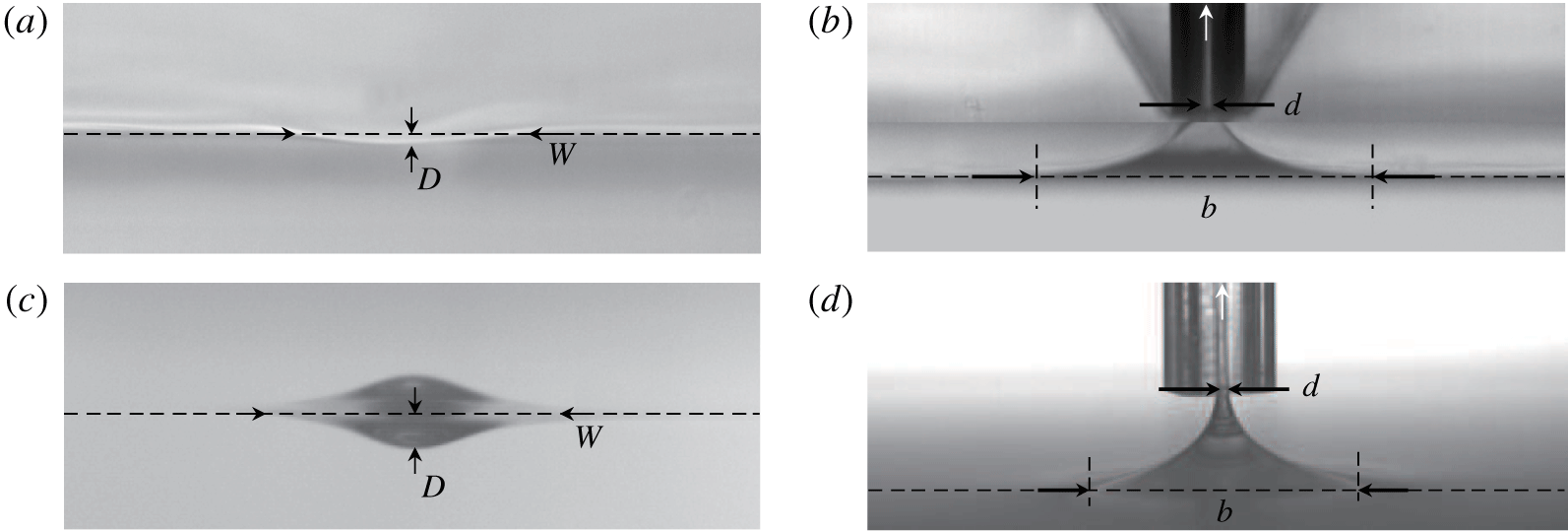
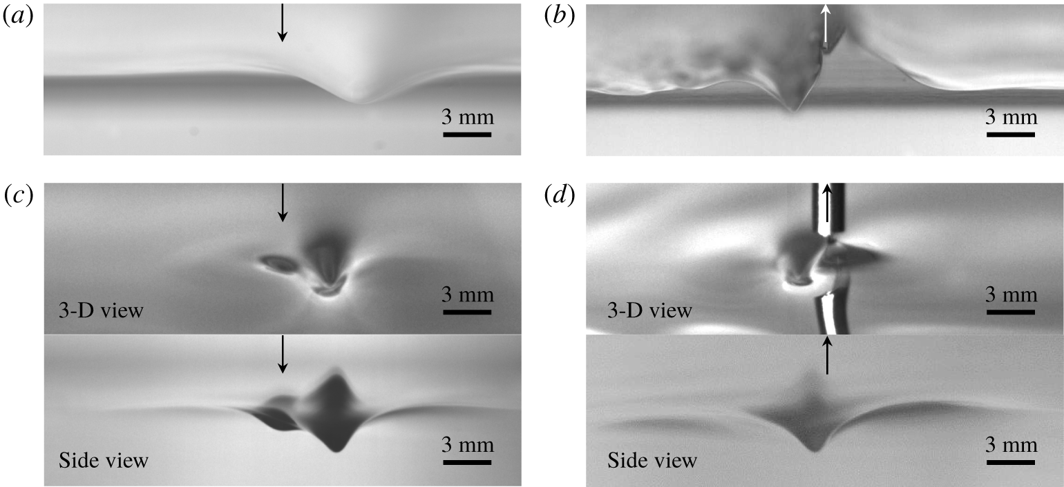
Experimental set-ups for the present 2-D/3-D air-blowing/air-suction experiments are schematically shown in figure 1, and are the same as the present authors’ 2-D air-blowing experimental work (Park & Cho Reference Park and Cho2018) and 3-D air-suction experimental work (Park & Cho Reference Park and Cho2016); an air-blowing compressor is used for the air-blowing test and a vacuum cleaner is used for the air-suction test. For more details about relevant experimental set-ups and observation techniques, interested readers are recommended to refer to these works. The degree of 2-D/3-D air blowing/air suction is determined when the forcing is stationary. For 2-D/3-D air-blowing cases, when the air-blowing forcing is stationary, the degree of air blowing is represented by the slope of a 2-D/3-D depression on the water surface, i.e. the dimensionless parameter  $\unicode[STIX]{x1D716}=D/W$, where
 $D$ is the depth of the depression and
 $W$ is the width or diameter of the depression, which is the distance between two points where the depression profile meets the horizontal free surface (figures 2a and 2c). As the degree of air blowing increases (decreases),
 $D$ increases (decreases) and
 $W$ changes little. Therefore, a stronger/weaker air-blowing forcing corresponds to a relatively higher/lower value of
 $\unicode[STIX]{x1D716}$. In the present work,
 $\unicode[STIX]{x1D716}=0.06$ (
 $D=0.48$ mm,
 $W=8.35$ mm),
 $\unicode[STIX]{x1D716}=0.08$ (
 $D=0.65$ mm,
 $W=8.06$ mm),
 $\unicode[STIX]{x1D716}=0.1$ (
 $D=0.78$ mm,
 $W=7.76$ mm) and
 $\unicode[STIX]{x1D716}=0.11$ (
 $D=0.84$ mm,
 $W=7.64$ mm) for 2-D air-blowing cases,
 $\unicode[STIX]{x1D716}=0.09$ (
 $D=0.68$ mm,
 $W=7.64$ mm),
 $\unicode[STIX]{x1D716}=0.11$ (
 $D=0.84$ mm,
 $W=7.64$ mm),
 $\unicode[STIX]{x1D716}=0.13$ (
 $D=1$ mm,
 $W=7.8$ mm) and
 $\unicode[STIX]{x1D716}=0.15$ (
 $D=1.2$ mm,
 $W=8$ mm) for 3-D air-blowing cases. For 2-D/3-D air-suction cases, when the air-suction forcing is stationary, the degree of the air suction is represented by the dimensionless parameter
 $\unicode[STIX]{x1D6FE}=d/b$, where
 $d$ is the width (2-D) or diameter (3-D) of a water column and
 $b$ is the base width (2-D) or diameter (3-D) of a water hump (figures 2b and 2d). As the degree of air suction increases (decreases),
 $b$ decreases (increases) and
 $d$ increases (decreases). Therefore, a stronger/weaker air-suction forcing corresponds to a relatively higher/lower value of
 $\unicode[STIX]{x1D6FE}$. In the present work,
 $\unicode[STIX]{x1D6FE}=0.04$ (
 $d=0.28$ mm,
 $b=7$ mm),
 $\unicode[STIX]{x1D6FE}=0.07$ (
 $d=0.48$ mm,
 $b=6.58$ mm),
 $\unicode[STIX]{x1D6FE}=0.1$ (
 $d=0.6$ mm,
 $b=6$ mm) and
 $\unicode[STIX]{x1D6FE}=0.12$ (
 $d=0.66$ mm,
 $b=5.5$ mm) for 2-D air-suction cases,
 $\unicode[STIX]{x1D6FE}=0.04$ (
 $d=0.3$ mm,
 $b=7.32$ mm),
 $\unicode[STIX]{x1D6FE}=0.07$ (
 $d=0.5$ mm,
 $b=6.85$ mm),
 $\unicode[STIX]{x1D6FE}=0.1$ (
 $d=0.66$ mm,
 $b=6.6$ mm) and
 $\unicode[STIX]{x1D6FE}=0.14$ (
 $d=0.84$ mm,
 $b=6$ mm) for 3-D air-suction cases. For visualization of surface-wave patterns, the shadowgraph technique was adopted and pictures were recorded on a carriage-attached high-speed camera according to the dimensionless forcing speed (
 $\unicode[STIX]{x1D6FC}=U/c_{min}$) for several forcing magnitudes.
The degree of a 2-D/3-D air blowing/air suction when the forcing is stationary. (a) The degree of a 2-D air blowing ( $\unicode[STIX]{x1D716}=D$/
 $W$:
 $D$, depth of the depression;
 $W$, width of the depression). (b) The degree of a 2-D air suction (
 $\unicode[STIX]{x1D6FE}=d/b$:
 $d$, width of the water column;
 $b$, base width of a water hump). (c) The degree of a 3-D air blowing (
 $\unicode[STIX]{x1D716}=D/W$:
 $D$, depth of the depression;
 $W$, width of the depression). In the picture, the upper part is the reflected image of the lower depression wave. (d) The degree of a 3-D air suction (
 $\unicode[STIX]{x1D6FE}=d/b$:
 $d$, diameter of the water column;
 $b$, base diameter of a water hump).

3 Experimental results: hysteresis phenomena
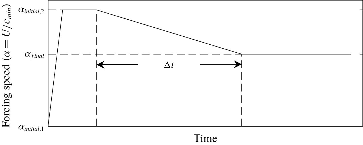
Prescribed speed variation of a forcing during the hysteresis experiment, where  $\unicode[STIX]{x1D6FC}_{initial,1}=U_{initial,1}/c_{min}=0$,
 $\unicode[STIX]{x1D6FC}_{initial,2}=U_{initial,2}/c_{min}$ and
 $\unicode[STIX]{x1D6FC}_{final}=U_{final}/c_{min}$.

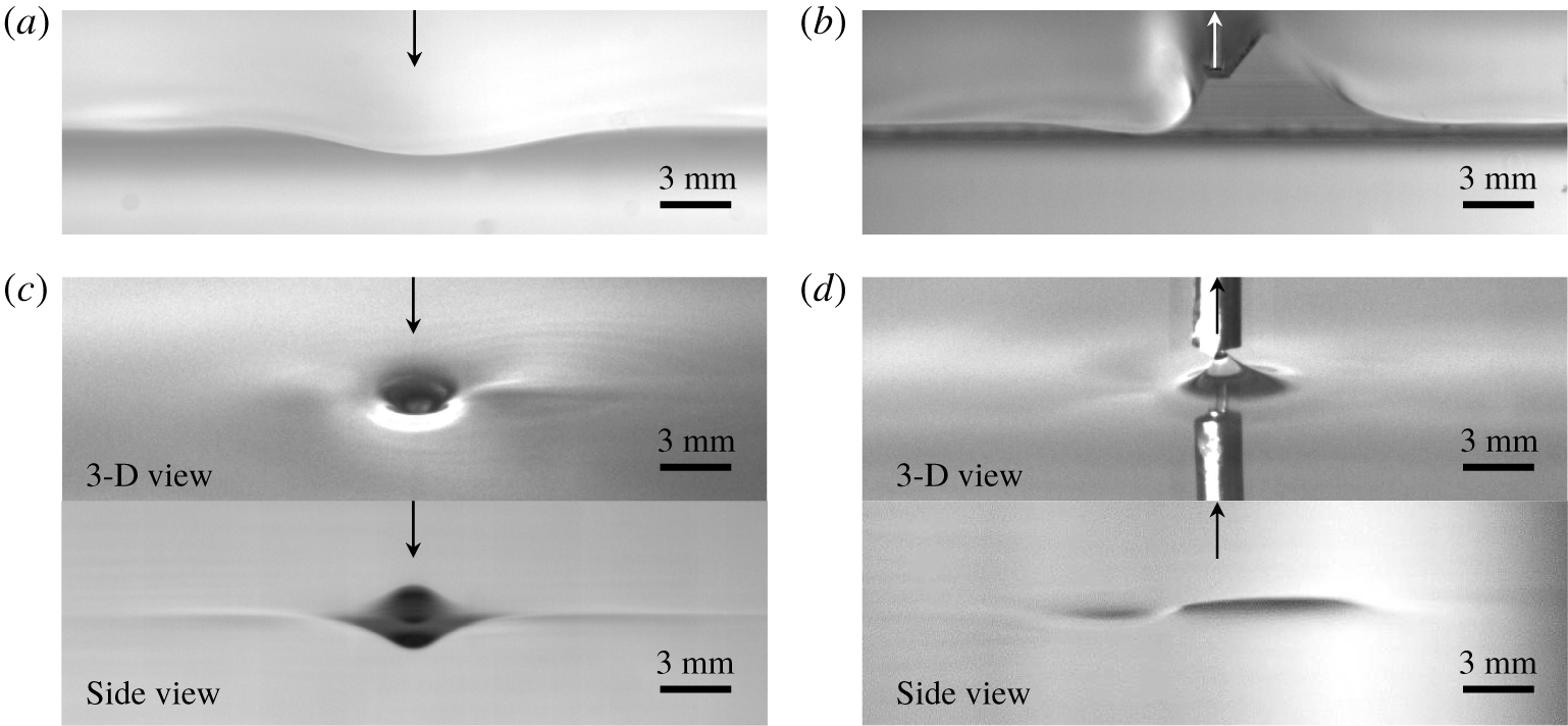
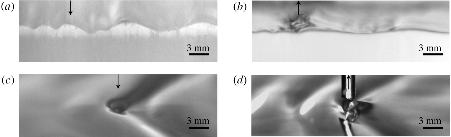
State I: Steady linear small-amplitude 2-D/3-D localized depressions. Arrows represent forcings. Panel (a) shows 2-D blowing ( $\unicode[STIX]{x1D6FC}=0.87$,
 $\unicode[STIX]{x1D716}=0.06$); (b) 2-D suction (
 $\unicode[STIX]{x1D6FC}=0.87$,
 $\unicode[STIX]{x1D6FE}=0.04$); (c) 3-D blowing (
 $\unicode[STIX]{x1D6FC}=0.87$,
 $\unicode[STIX]{x1D716}=0.09$) and (d) 3-D suction (
 $\unicode[STIX]{x1D6FC}=0.87$,
 $\unicode[STIX]{x1D6FE}=0.04$).

State II: Steady nonlinear finite-amplitude 2-D/3-D gravity–capillary solitary waves (a,c,d) or 2-D steady localized depressions (b). Arrows represent forcings. Panel (a) shows 2-D blowing ( $\unicode[STIX]{x1D6FC}=0.92$,
 $\unicode[STIX]{x1D716}=0.06$); (b) 2-D suction (
 $\unicode[STIX]{x1D6FC}=0.92$,
 $\unicode[STIX]{x1D6FE}=0.04$); (c) 3-D blowing (
 $\unicode[STIX]{x1D6FC}=0.96$,
 $\unicode[STIX]{x1D716}=0.09$); and (d) 3-D suction (
 $\unicode[STIX]{x1D6FC}=0.96$,
 $\unicode[STIX]{x1D6FE}=0.04$).

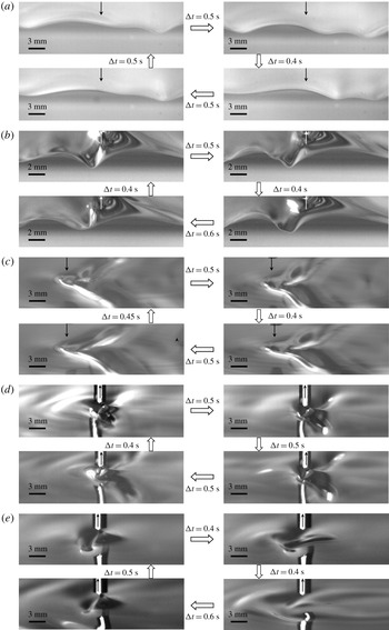
State III: Periodic shedding of 2-D/3-D gravity–capillary localized depressions (a–d) or repeated ‘snap-stick’ phenomena (e). Arrows represent forcings. Panel (a) shows 2-D blowing ( $\unicode[STIX]{x1D6FC}=1$,
 $\unicode[STIX]{x1D716}=0.06$); (b) 2-D suction (
 $\unicode[STIX]{x1D6FC}=1$,
 $\unicode[STIX]{x1D6FE}=0.04$); (c) 3-D blowing (
 $\unicode[STIX]{x1D6FC}=1$,
 $\unicode[STIX]{x1D716}=0.09$); (d) 3-D suction (
 $\unicode[STIX]{x1D6FC}=1$,
 $\unicode[STIX]{x1D6FE}=0.04$); and (e) 3-D suction (
 $\unicode[STIX]{x1D6FC}=0.99$,
 $\unicode[STIX]{x1D6FE}=0.04$).

State IV: Steady linear 2-D/3-D gravity–capillary waves. Arrows represent forcings. Panel (a) shows 2-D blowing ( $\unicode[STIX]{x1D6FC}=1.1$,
 $\unicode[STIX]{x1D716}=0.06$); (b) 2-D suction (
 $\unicode[STIX]{x1D6FC}=1.1$,
 $\unicode[STIX]{x1D6FE}=0.04$); (c) 3-D blowing (
 $\unicode[STIX]{x1D6FC}=1.05$,
 $\unicode[STIX]{x1D716}=0.09$); and (d) 3-D suction (
 $\unicode[STIX]{x1D6FC}=1.05$,
 $\unicode[STIX]{x1D6FE}=0.04$).

A carriage was fixed to a belt-pulley system that was servomotor-controlled and programmed such that the carriage will move from right to left with a prescribed speed variation as shown in figure 3. The speed variation curve comprises four parts: a constant acceleration phase from a stationary state (zero speed  $\unicode[STIX]{x1D6FC}_{initial,1}=U_{initial,1}/c_{min}=0$) towards a first target speed (
 $\unicode[STIX]{x1D6FC}_{initial,2}=U_{initial,2}/c_{min}$), a zero acceleration phase (
 $\unicode[STIX]{x1D6FC}=\unicode[STIX]{x1D6FC}_{initial,2}$) after the first target speed is obtained, a constant deceleration phase from the first target speed towards the second target speed (
 $\unicode[STIX]{x1D6FC}_{final}=U_{final}/c_{min}$) and a zero acceleration phase (
 $\unicode[STIX]{x1D6FC}=\unicode[STIX]{x1D6FC}_{final}$) after the second target speed is obtained. During the acceleration phase (
 $\unicode[STIX]{x1D6FC}_{initial,1}=0\rightarrow \unicode[STIX]{x1D6FC}_{initial,2}$) and the subsequent constant-speed phase (
 $\unicode[STIX]{x1D6FC}_{initial,2}\rightarrow \unicode[STIX]{x1D6FC}_{initial,2}$), for an initial still-water condition, states I, II, III and IV were generated by 2-D/3-D air-blowing/air-suction forcings (figures 4–7). It was observed that the duration time during the acceleration, i.e. the time taken to accelerate from zero to the first target speed, does not affect the resultant waves at speed
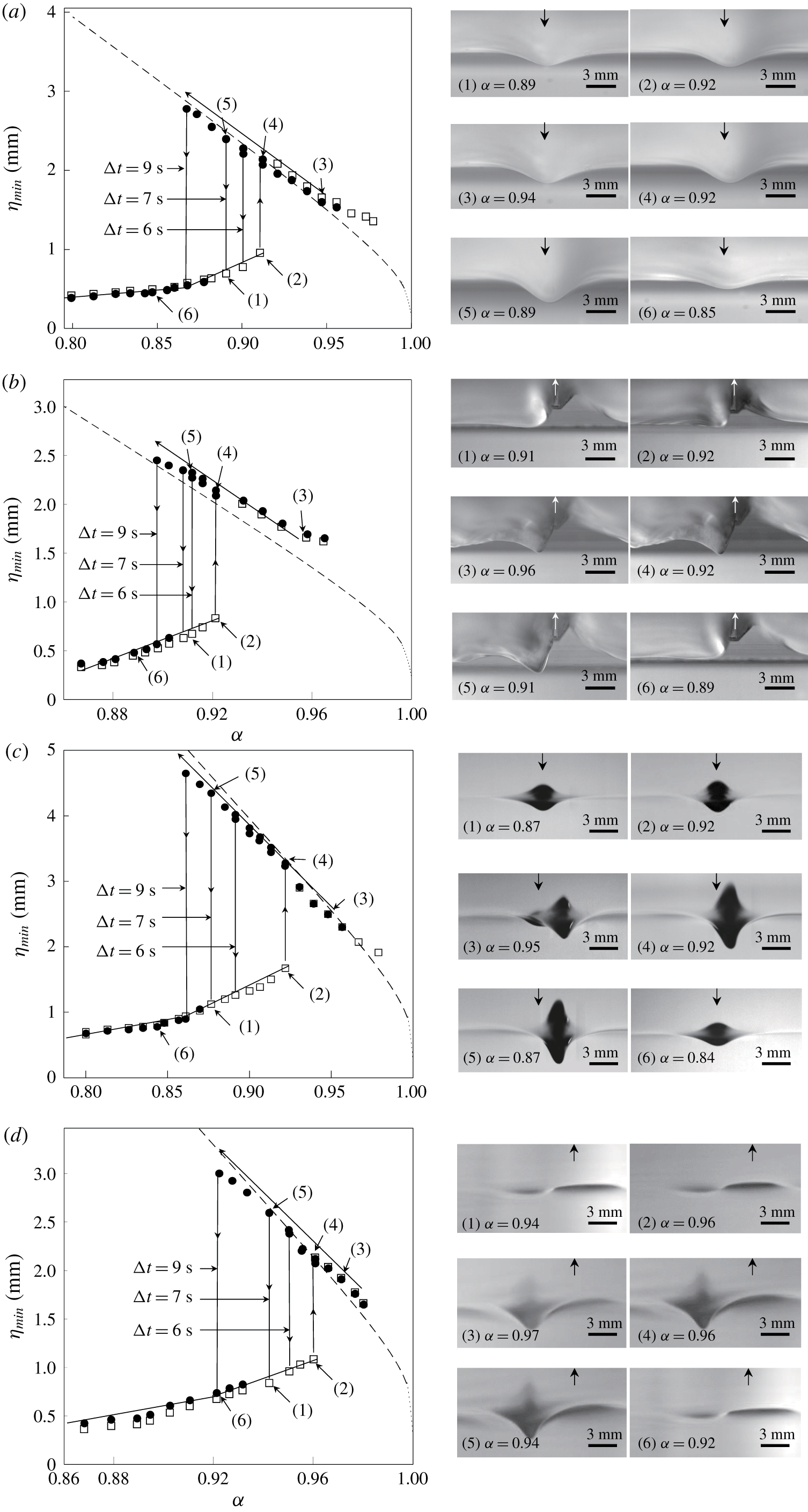
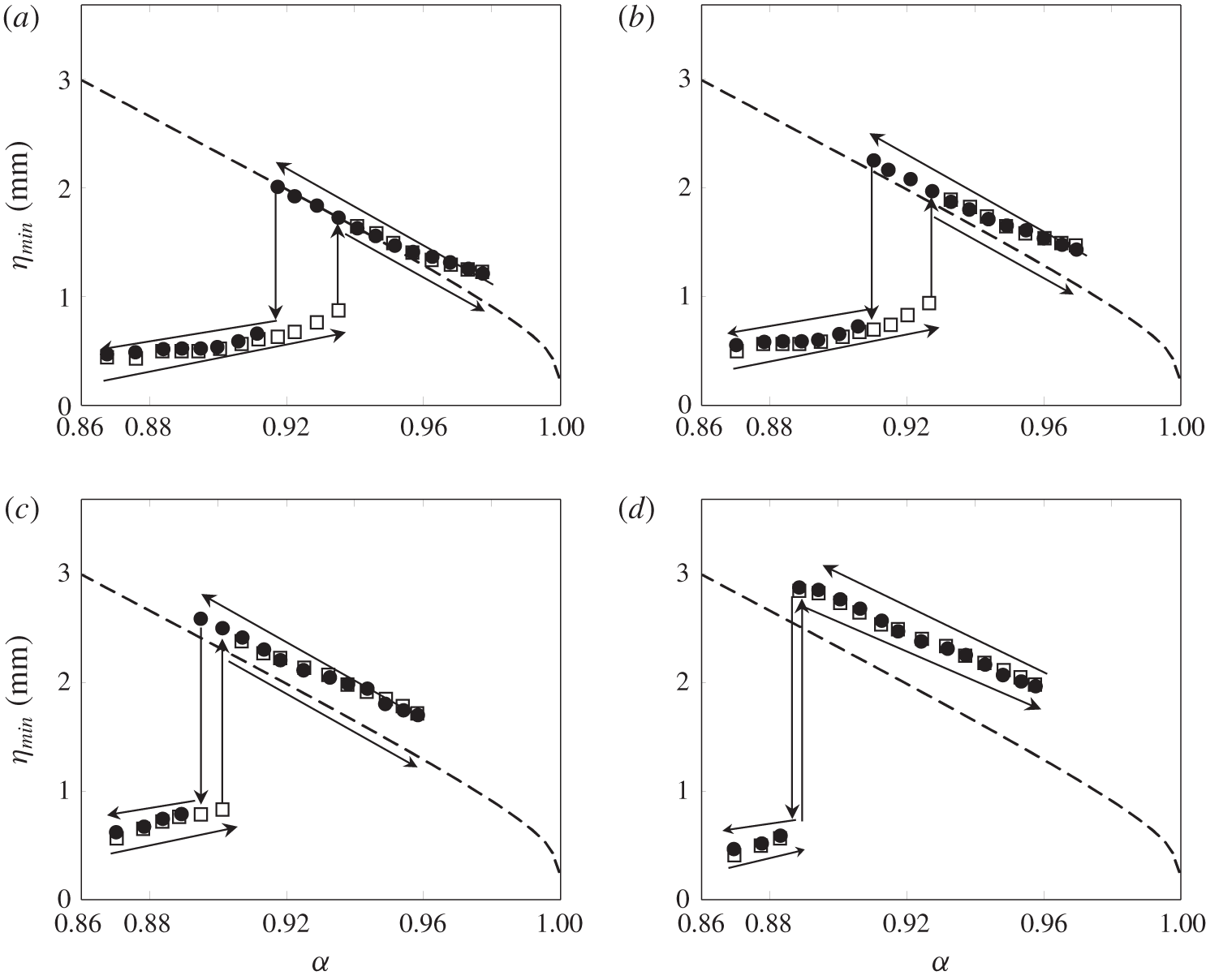
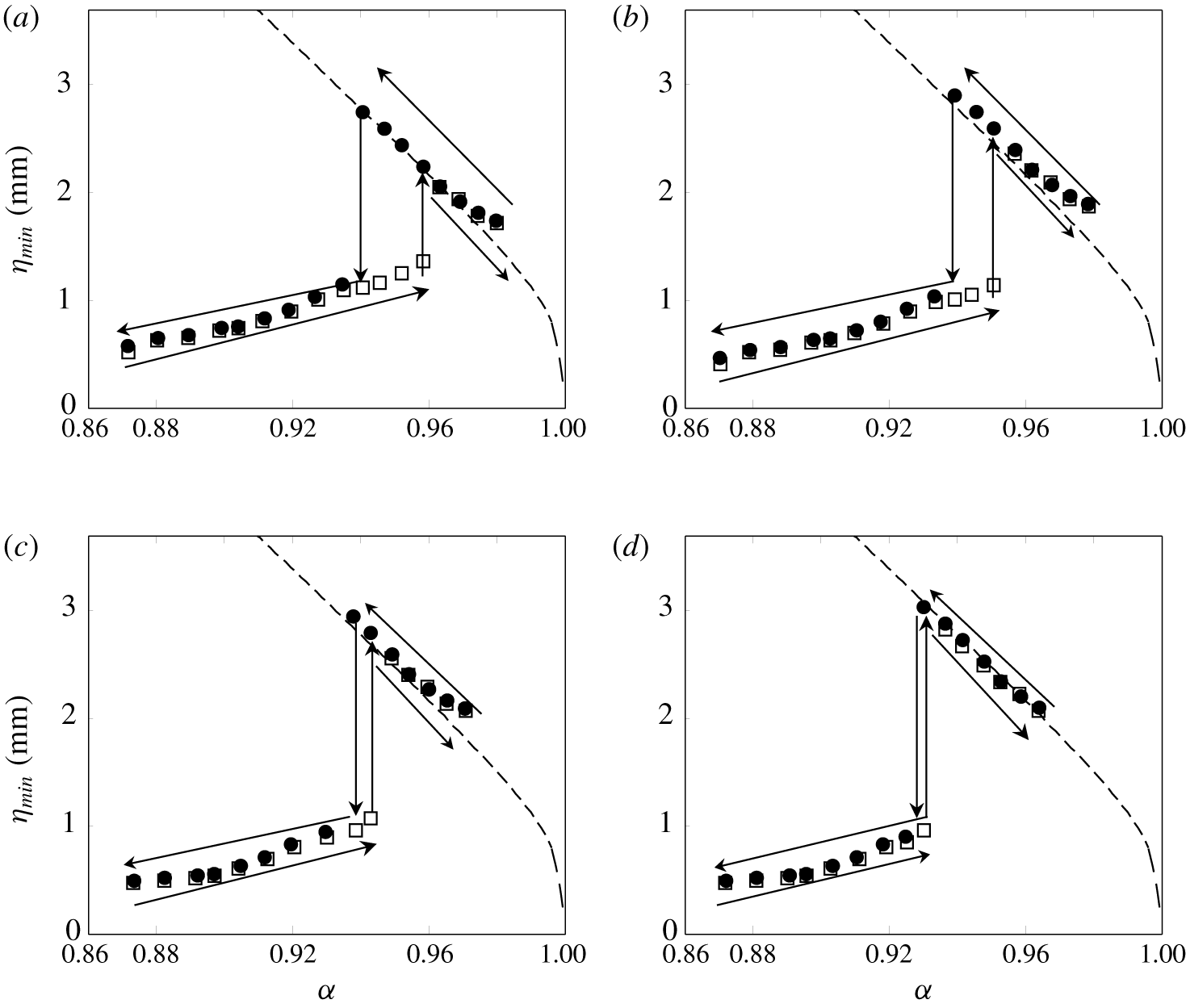
 $\unicode[STIX]{x1D6FC}_{initial,2}$. Therefore, considering the length limit of the tank, the shortest possible duration time (around 0.6 s) during the acceleration was used throughout the experiment. For steady localized linear state I and nonlinear state II, in particular, the relation between the forcing speed and the maximum depression of the resultant steady waves is shown in the steady response diagrams (figures 8a–8d). As can be seen from the square symbols (▫) in figures 8(a)–8(d), as the forcing speed increases from zero towards a certain target constant speed (
 $\unicode[STIX]{x1D6FC}_{initial,1}=0\rightarrow \unicode[STIX]{x1D6FC}_{initial,2}$), there exists a certain critical speed (
 $\unicode[STIX]{x1D6FC}_{crit}$) below which linear state I is observed (
 $\unicode[STIX]{x1D6FC}_{initial,2}<\unicode[STIX]{x1D6FC}_{crit}$) and above which nonlinear state II is observed (
 $\unicode[STIX]{x1D6FC}_{initial,2}>\unicode[STIX]{x1D6FC}_{crit}$). As will be shown in the next section, the critical speed (
 $\unicode[STIX]{x1D6FC}_{crit}$) is the so-called first turning point predicted from the response diagram, which shows the relationship between the forcing speed and the maximum depression of the localized wave solutions to a model equation. As mentioned in the introduction, these kinds of experiments were already carried out in several existing works: for 2-D air-blowing (Park & Cho Reference Park and Cho2018), for 3-D air-blowing (Diorio et al. Reference Diorio, Cho, Duncan and Akylas2009, Reference Diorio, Cho, Duncan and Akylas2011; Masnadi & Duncan Reference Masnadi and Duncan2017a,Reference Masnadi and Duncanb) and for 3-D air-suction cases (Park & Cho Reference Park and Cho2016). In figures 8(a)–8(d), the dashed curves represent 2-D/3-D inviscid forcing-free gravity–capillary solitary waves that are the solutions to the dimensionless model equations (A 1)–(A 5) in appendix A. Next, constant-speed states with
 $\unicode[STIX]{x1D6FC}=\unicode[STIX]{x1D6FC}_{initial,2}$ (states I, II, III and IV) will go through the subsequent deceleration phase (
 $\unicode[STIX]{x1D6FC}_{initial,2}\rightarrow \unicode[STIX]{x1D6FC}_{final}<\unicode[STIX]{x1D6FC}_{crit}$) and, subsequently, constant-speed phase (
 $\unicode[STIX]{x1D6FC}_{final}\rightarrow \unicode[STIX]{x1D6FC}_{final}$). In other words, the new initial conditions will be states I, II, III and IV with
 $\unicode[STIX]{x1D6FC}=\unicode[STIX]{x1D6FC}_{initial,2}$. For state-I initial conditions (figure 4), final states are also state I. For state-II initial conditions, as marked by circles (●) in figures 8(a)–8(d), as the forcing speed is decreased from
 $\unicode[STIX]{x1D6FC}_{initial,2}=0.96$ (state II in figure 5) towards a final forcing speed
 $\unicode[STIX]{x1D6FC}_{final}$ (
 ${<}\unicode[STIX]{x1D6FC}_{crit}$) with a deceleration time
 $\unicode[STIX]{x0394}t=7$ s, steeper 2-D/3-D gravity–capillary solitary waves (2-D/3-D air-blowing and 3-D air-suction cases) or steeper 2-D localized depressions (2-D air-suction case) are observed (if
 $\unicode[STIX]{x1D6FC}_{final}>\unicode[STIX]{x1D6FC}_{crit}$, final states will be already obtained states II). These nonlinear waves, however, cannot be observed for speeds far below the critical speed (
 $\unicode[STIX]{x1D6FC}_{crit}$), and, below a certain forcing speed (
 $\unicode[STIX]{x1D6FC}_{crit,2}$), state-I waves are observed instead. For state-III (figure 6) and state-IV (figure 7) initial conditions, similar phenomena to those for state-II initial conditions are observed. In summary, two kinds of jump transitions (from linear to nonlinear states at a certain critical speed and from nonlinear to linear states at another critical speed) can be identified, showing the dependence of a state on its history starting from different initial conditions. These are hysteresis phenomena in 2-D/3-D gravity–capillary waves generated by 2-D/3-D air-blowing/air-suction forcings. Similar experiments were carried out for a relatively short duration time,
 $\unicode[STIX]{x0394}t=6$ s, and a long duration time,
 $\unicode[STIX]{x0394}t=9$ s, during the deceleration. As the duration time increases (slow deceleration), the downward jump speed (
 $\unicode[STIX]{x1D6FC}_{crit}$) – at which the transition from nonlinear to linear states occurs – becomes farther from the upward jump speed (
 $\unicode[STIX]{x1D6FC}_{crit,2}$), as shown in figure 8.
Maximum depression of the resultant steady waves versus forcing speed ( $\unicode[STIX]{x1D6FC}$). Dashed curves, inviscid forcing-free equation (A 1) for 2-D cases and (A 2) for 3-D cases. Symbols: ▫, final steady waves when the forcing speed increases from zero (
 $\unicode[STIX]{x1D6FC}_{initial,1}=0$) towards a certain target constant speed (
 $\unicode[STIX]{x1D6FC}_{initial,2}$); ●, final steady waves when the forcing speed is decreased from
 $\unicode[STIX]{x1D6FC}_{initial,2}$ (
 $\unicode[STIX]{x1D6FC}_{initial,2}>\unicode[STIX]{x1D6FC}_{crit}$) towards a certain below-critical speed (
 $\unicode[STIX]{x1D6FC}_{final}<\unicode[STIX]{x1D6FC}_{crit}$), where the initial condition is state II and the decelerating duration times are
 $\unicode[STIX]{x0394}t=6$ s, 7 s and 9 s. Panel (a) shows 2-D blowing (
 $\unicode[STIX]{x1D716}=0.06$); (b) 2-D suction (
 $\unicode[STIX]{x1D6FE}=0.04$); (c) 3-D blowing (
 $\unicode[STIX]{x1D716}=0.09$); and (d) 3-D suction (
 $\unicode[STIX]{x1D6FE}=0.04$).

4 Comparison between experiments and simulations: 2-D/3-D air-blowing cases
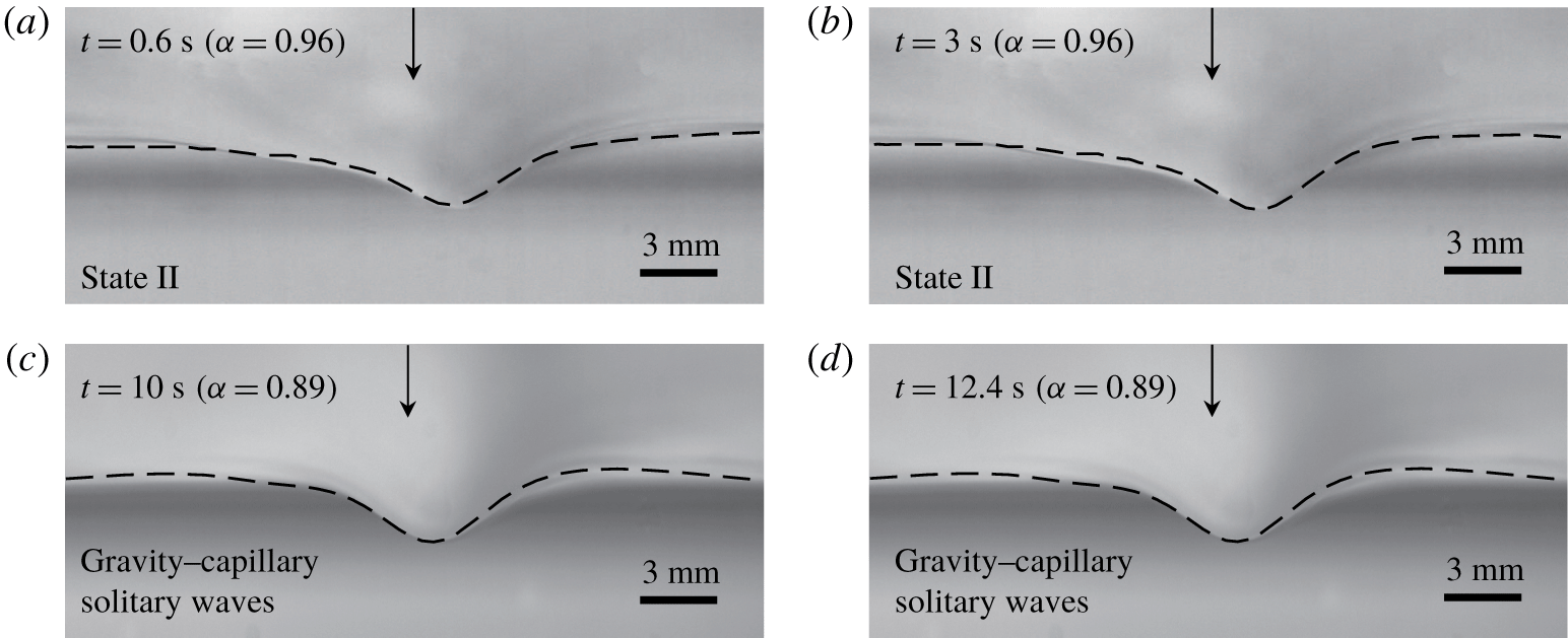
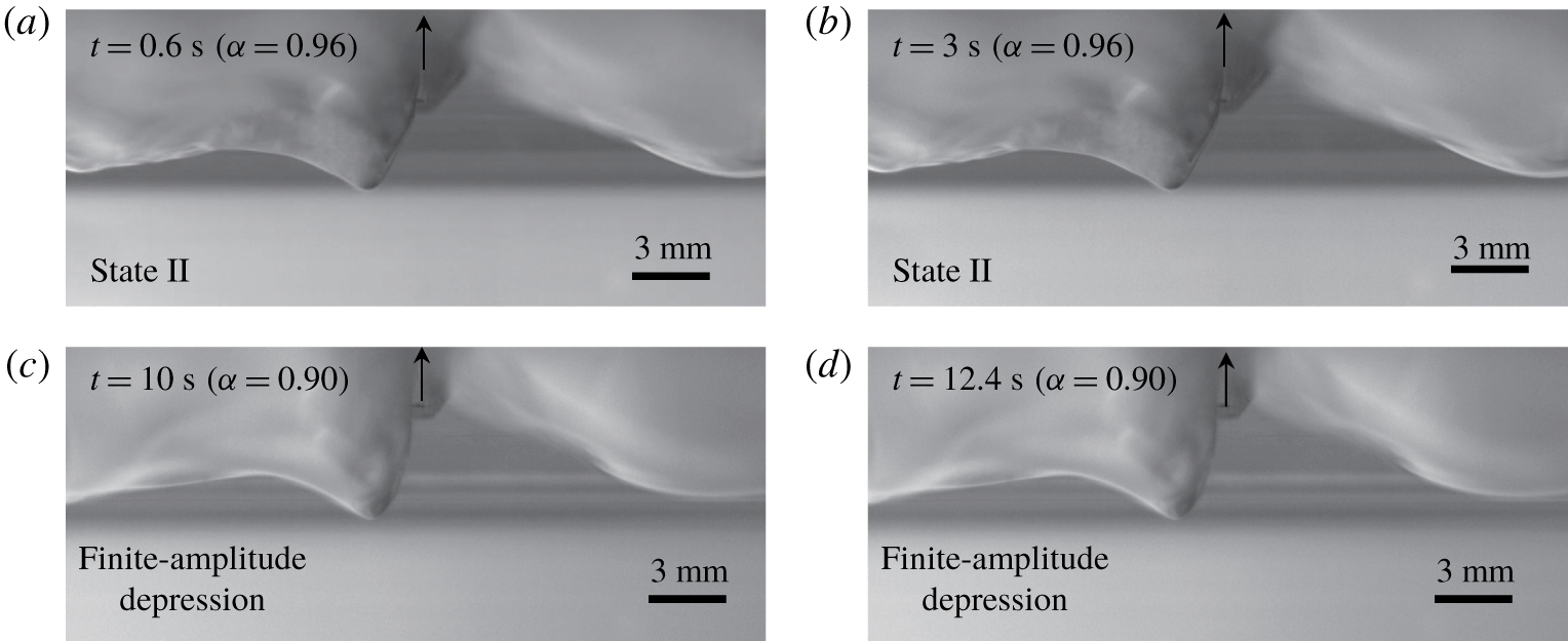
Side-view wave profiles according to the variation of 2-D air-blowing forcing speed ( $\unicode[STIX]{x1D6FC}_{initial,1}=0~(t=0~\text{s})\rightarrow \unicode[STIX]{x1D6FC}_{initial,2}~(t=0.6{-}3~\text{s})\rightarrow \unicode[STIX]{x1D6FC}_{final}~(t=10{-}13~\text{s})$) where the intermediate initial condition is the state-II wave at
 $\unicode[STIX]{x1D6FC}_{initial,2}=0.96$. Simulation results (dashed curves,
 $A=0.036$) are overlaid on the experimental pictures (
 $\unicode[STIX]{x1D716}=0.06$).

For a better understanding of the hysteresis phenomena observed in the experiment, particularly for 2-D/3-D air-blowing cases, comparisons will be made with simulation results based on the following dimensionless 2-D/3-D viscous, forced-model equations. The detailed derivation can be found in the present corresponding author’s previous works (Cho et al. Reference Cho, Diorio, Akylas and Duncan2011; Park & Cho Reference Park and Cho2016, Reference Park and Cho2018; Cho Reference Cho2018):
 $$\begin{eqnarray}\displaystyle & \displaystyle \unicode[STIX]{x1D702}_{t}+\unicode[STIX]{x1D6FC}\unicode[STIX]{x1D702}_{x}-{\textstyle \frac{1}{2}}\unicode[STIX]{x1D702}_{x}-{\textstyle \frac{1}{4}}\mathscr{H}\{\unicode[STIX]{x1D702}_{xx}-\unicode[STIX]{x1D702}\}-\unicode[STIX]{x1D6FD}(\unicode[STIX]{x1D702}^{2})_{x}-\widetilde{\unicode[STIX]{x1D708}}\unicode[STIX]{x1D702}_{xx}=Ap_{x},\quad (\text{2-D}), & \displaystyle\end{eqnarray}$$
 $$\begin{eqnarray}\displaystyle & \displaystyle \underbrace{\unicode[STIX]{x1D702}_{t}+\unicode[STIX]{x1D6FC}\unicode[STIX]{x1D702}_{x}}_{convection}\underbrace{-{\textstyle \frac{1}{2}}\unicode[STIX]{x1D702}_{x}-{\textstyle \frac{1}{4}}\mathscr{H}\{\unicode[STIX]{x1D702}_{xx}+2\unicode[STIX]{x1D702}_{yy}-\unicode[STIX]{x1D702}\}}_{dispersion}\underbrace{-\unicode[STIX]{x1D6FD}(\unicode[STIX]{x1D702}^{2})_{x}}_{\substack{ nonlinear \\ steepening}}\underbrace{-\widetilde{\unicode[STIX]{x1D708}}(\unicode[STIX]{x1D702}_{xx}+\unicode[STIX]{x1D702}_{yy})}_{\substack{ viscous \\ dissipation}}=\underbrace{Ap_{x}}_{forcing},\quad (\text{3-D}),\quad & \displaystyle\end{eqnarray}$$
where  $\unicode[STIX]{x1D702}(x,t)$ and
 $\unicode[STIX]{x1D702}(x,y,t)$ are the dimensionless wave solutions to (4.1) and (4.2), respectively,
 $t$ is the dimensionless time,
 $\widetilde{\unicode[STIX]{x1D708}}=C\unicode[STIX]{x1D708}(4g)^{1/4}(\unicode[STIX]{x1D70C}/\unicode[STIX]{x1D70E})^{3/4}$, where
 $\unicode[STIX]{x1D708}$ is the kinematic viscosity of water,
 $C=2.4$ is the tuning parameter which is found to give the best agreement between the computational results and the experimental results in terms of speed-dependent behaviours both qualitatively and quantitatively (Cho et al. Reference Cho, Diorio, Akylas and Duncan2011; Park & Cho Reference Park and Cho2016, Reference Park and Cho2018; Cho Reference Cho2018),
 $A$ is the forcing magnitude and
 $p(x)$ and
 $p(x,y)$ are the following forcing functions:
 $$\begin{eqnarray}\displaystyle & \displaystyle p(x)=\text{exp}(-2x^{2}),\quad (\text{2-D}), & \displaystyle\end{eqnarray}$$
 $$\begin{eqnarray}\displaystyle & \displaystyle p(x,y)=\text{exp}(-2x^{2}-2y^{2}),\quad (\text{3-D}). & \displaystyle\end{eqnarray}$$
Equations (4.1) and (4.3) for 2-D air-blowing cases and (4.2) and (4.4) for 3-D air-blowing cases are solved using spectral methods (Cho et al. Reference Cho, Diorio, Akylas and Duncan2011; Park & Cho Reference Park and Cho2016; Cho Reference Cho2018) with still-water initial conditions and time-varying speed  $\unicode[STIX]{x1D6FC}(t)$, as shown in figure 3. For a dimensional result, the characteristic length
 $L=2.73$ mm and the characteristic time
 $T=L/c_{min}=0.0118$ s will be multiplied to the dimensionless length and time, respectively. First, starting from still-water initial conditions, the forcing speed (
 $\unicode[STIX]{x1D6FC}$) is increased until
 $\unicode[STIX]{x1D6FC}_{initial,2}=0.96$, 1 and 1.1 (2-D blowing cases) and
 $\unicode[STIX]{x1D6FC}_{initial,2}=0.96$, 1 and 1.05 (3-D blowing cases) are reached (duration time
 $\unicode[STIX]{x0394}t=0.6$ s during the acceleration) and is maintained there for 2.4 s. Then, states II, III and IV for
 $\unicode[STIX]{x1D6FC}_{initial,2}=0.96$, 1 and 1.1 (2-D blowing cases) and
 $\unicode[STIX]{x1D6FC}_{initial,2}=0.96$, 1 and 1.05 (3-D blowing cases), respectively, are generated in the experiment and are numerically obtained in the transient simulation of (4.1) and (4.3) for 2-D air-blowing cases and (4.2) and (4.4) for 3-D air-blowing cases; in the experiment,
 $\unicode[STIX]{x1D716}=0.06$ (2-D) and
 $\unicode[STIX]{x1D716}=0.09$ (3-D) and, in the simulation,
 $A=0.036$ (2-D) and
 $A=0.23$ (3-D) are used. Then, with these state-II, III and IV initial conditions, the forcing speed (
 $\unicode[STIX]{x1D6FC}$) is decreased until
 $\unicode[STIX]{x1D6FC}_{final}=0.89$ (2-D blowing cases) and
 $\unicode[STIX]{x1D6FC}_{final}=0.87$ (3-D blowing cases) are reached (duration time
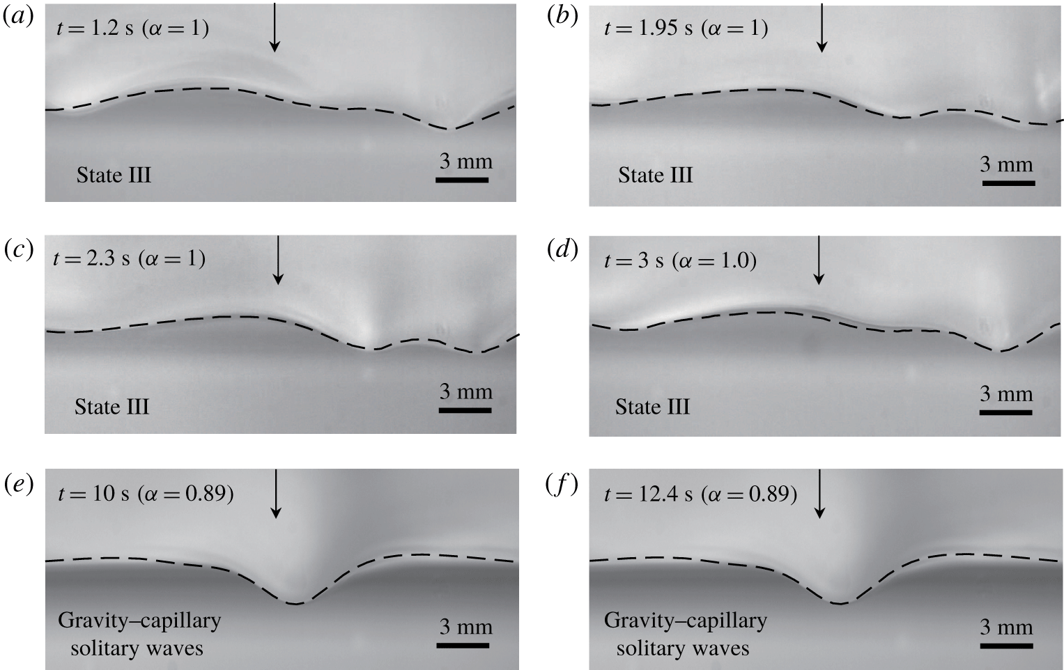
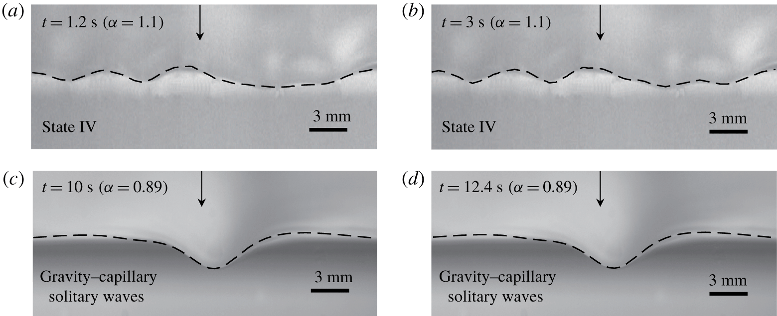
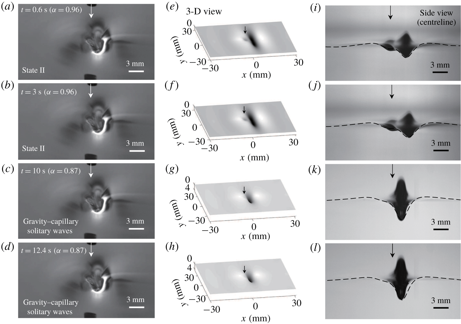
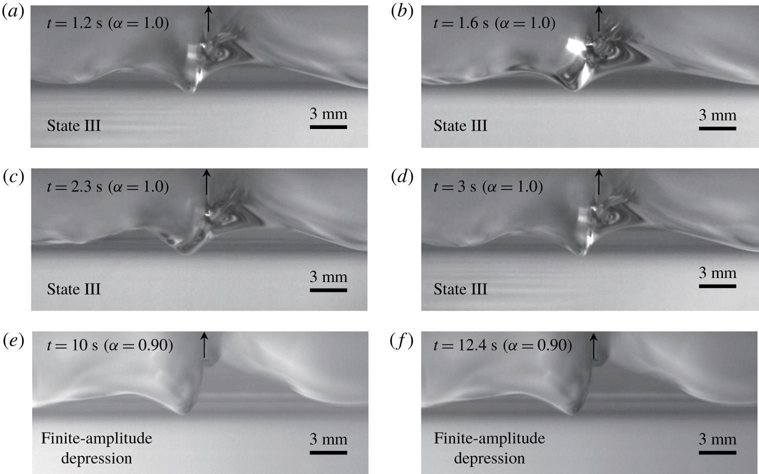
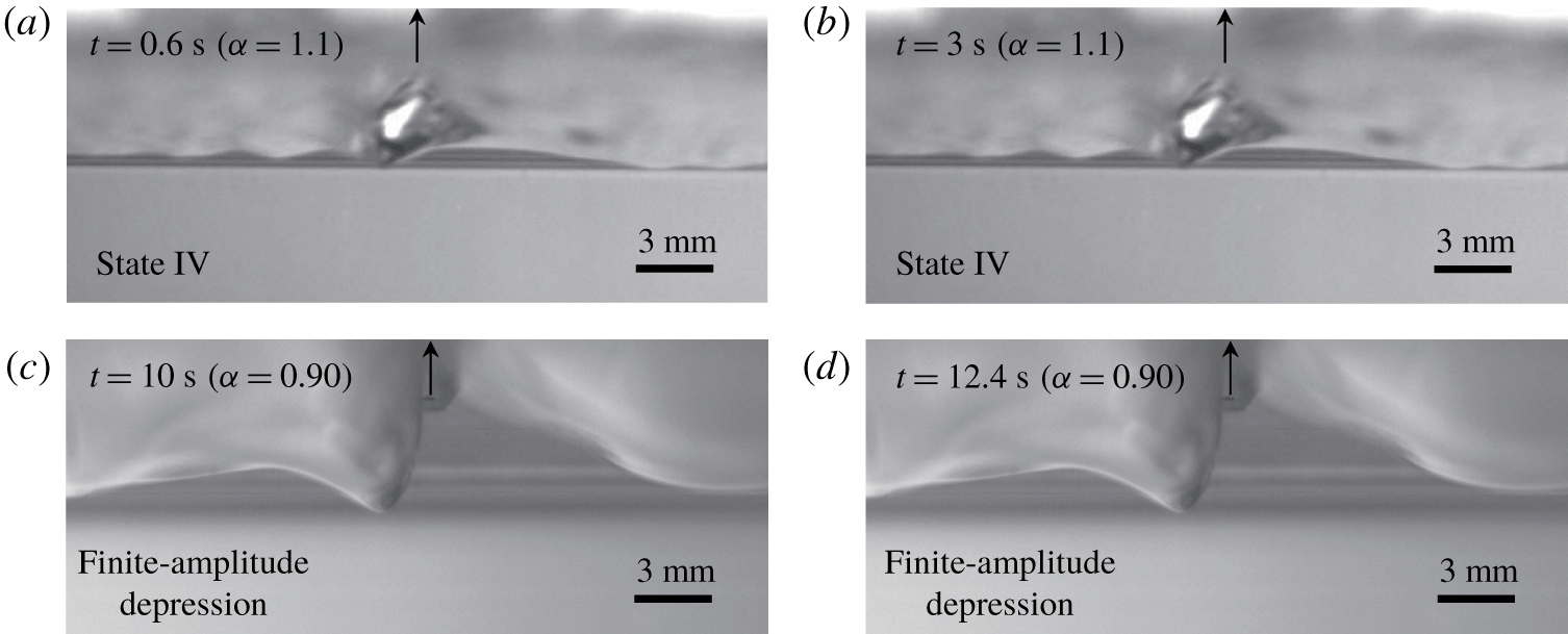
 $\unicode[STIX]{x0394}t=7$ s during the deceleration) and is maintained thereafter, both in the experiments and the transient simulations. The final steady states are steeper 2-D/3-D gravity–capillary solitary waves with
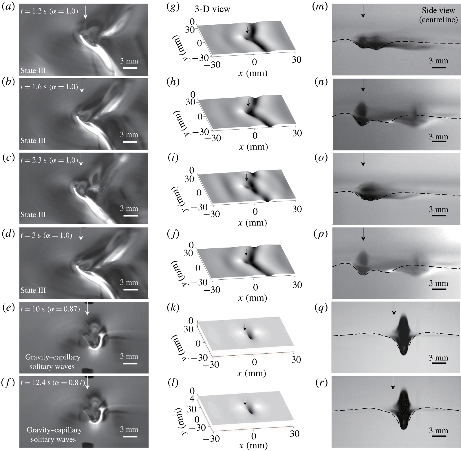
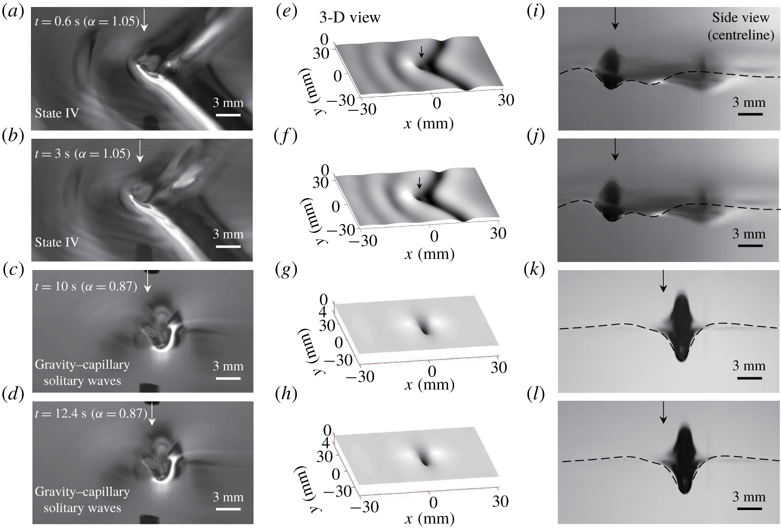
 $\unicode[STIX]{x1D6FC}_{final}=0.89$ (2-D) and 0.87 (3-D). Comparisons are shown in figures 9–11 for 2-D air-blowing and in figures 12–14 for 3-D air-blowing cases, respectively. In those figures, simulation results are overlaid on the experimental snapshots. They agree with each other very well. The experimental and the transient simulation results in figures 9–14 can be predicted from the response diagrams obtained from the solutions to the following steady-state version equations of (4.1) and (4.2):
 $$\begin{eqnarray}\displaystyle & \displaystyle \unicode[STIX]{x1D6FC}\unicode[STIX]{x1D702}_{x}-{\textstyle \frac{1}{2}}\unicode[STIX]{x1D702}_{x}-{\textstyle \frac{1}{4}}\mathscr{H}\{\unicode[STIX]{x1D702}_{xx}-\unicode[STIX]{x1D702}\}-\unicode[STIX]{x1D6FD}(\unicode[STIX]{x1D702}^{2})_{x}-\widetilde{\unicode[STIX]{x1D708}}\unicode[STIX]{x1D702}_{xx}=Ap_{x},\quad (\text{2-D}), & \displaystyle\end{eqnarray}$$
 $$\begin{eqnarray}\displaystyle & \displaystyle \underbrace{\unicode[STIX]{x1D6FC}\unicode[STIX]{x1D702}_{x}}_{convection}\underbrace{-{\textstyle \frac{1}{2}}\unicode[STIX]{x1D702}_{x}-{\textstyle \frac{1}{4}}\mathscr{H}\{\unicode[STIX]{x1D702}_{xx}+2\unicode[STIX]{x1D702}_{yy}-\unicode[STIX]{x1D702}\}}_{dispersion}\underbrace{-\unicode[STIX]{x1D6FD}(\unicode[STIX]{x1D702}^{2})_{x}}_{\substack{ nonlinear \\ steepening}}\underbrace{-\widetilde{\unicode[STIX]{x1D708}}(\unicode[STIX]{x1D702}_{xx}+\unicode[STIX]{x1D702}_{yy})}_{\substack{ viscous \\ dissipation}}=\underbrace{Ap_{x}}_{forcing},\quad (\text{3-D}).\quad & \displaystyle\end{eqnarray}$$
Side-view wave profiles according to the variation of 2-D air-blowing forcing speed ( $\unicode[STIX]{x1D6FC}_{initial,1}=0~(t=0~\text{s})\rightarrow \unicode[STIX]{x1D6FC}_{initial,2}~(t=0.6{-}3~\text{s})\rightarrow \unicode[STIX]{x1D6FC}_{final}~(t=10{-}13~\text{s})$) where the intermediate initial condition is the state-III wave at
 $\unicode[STIX]{x1D6FC}_{initial,2}=1$. Simulation results (dashed curves,
 $A=0.036$) are overlaid on the experimental pictures (
 $\unicode[STIX]{x1D716}=0.06$).

Side-view wave profiles according to the variation of 2-D air-blowing forcing speed ( $\unicode[STIX]{x1D6FC}_{initial,1}=0~(t=0~\text{s})\rightarrow \unicode[STIX]{x1D6FC}_{initial,2}~(t=0.6{-}3~\text{s})\rightarrow \unicode[STIX]{x1D6FC}_{final}~(t=10{-}13~\text{s})$) where the intermediate initial condition is the state-IV wave at
 $\unicode[STIX]{x1D6FC}_{initial,2}=1.1$. Simulation results (dashed curves,
 $A=0.036$) are overlaid on the experimental pictures (
 $\unicode[STIX]{x1D716}=0.06$).

Wave profiles according to the variation of 3-D air-blowing forcing speed ( $\unicode[STIX]{x1D6FC}_{initial,1}=0~(t=0~\text{s})\rightarrow \unicode[STIX]{x1D6FC}_{initial,2}~(t=0.6{-}3~\text{s})\rightarrow \unicode[STIX]{x1D6FC}_{final}~(t=10{-}13~\text{s})$) where the intermediate initial condition is the state-II wave at
 $\unicode[STIX]{x1D6FC}_{initial,2}=0.96$. (a–d) Experimental results (3-D view,
 $\unicode[STIX]{x1D716}=0.09$). (e–h) Simulation results (3-D view,
 $A=0.23$). (i–l) Experimental and simulation (dashed curves) results (side view).

Wave profiles according to the variation of 3-D air-blowing forcing speed ( $\unicode[STIX]{x1D6FC}_{initial,1}=0~(t=0~\text{s})\rightarrow \unicode[STIX]{x1D6FC}_{initial,2}~(t=0.6{-}3~\text{s})\rightarrow \unicode[STIX]{x1D6FC}_{final}~(t=10{-}13~\text{s})$) where the intermediate initial condition is the state-III wave at
 $\unicode[STIX]{x1D6FC}_{initial,2}=1$. (a–f) Experimental results (3-D view,
 $\unicode[STIX]{x1D716}=0.09$). (g–l) Simulation results (3-D view,
 $A=0.23$). (m–r) Experimental and simulation (dashed curves) results (side view).

Wave profiles according to the variation of 3-D air-blowing forcing speed ( $\unicode[STIX]{x1D6FC}_{initial,1}=0~(t=0~\text{s})\rightarrow \unicode[STIX]{x1D6FC}_{initial,2}~(t=0.6{-}3~\text{s})\rightarrow \unicode[STIX]{x1D6FC}_{final}~(t=10{-}13~\text{s})$) where the intermediate initial condition is the state-IV wave at
 $\unicode[STIX]{x1D6FC}_{initial,2}=1.05$. (a–d) Experimental results (3-D view,
 $\unicode[STIX]{x1D716}=0.09$). (e–h) Simulation results (3-D view,
 $A=0.23$). (i–l) Experimental and simulation (dashed curves) results (side view).

These equations are solved using the pseudo-arclength continuation method by treating both  $\unicode[STIX]{x1D6FC}$ and
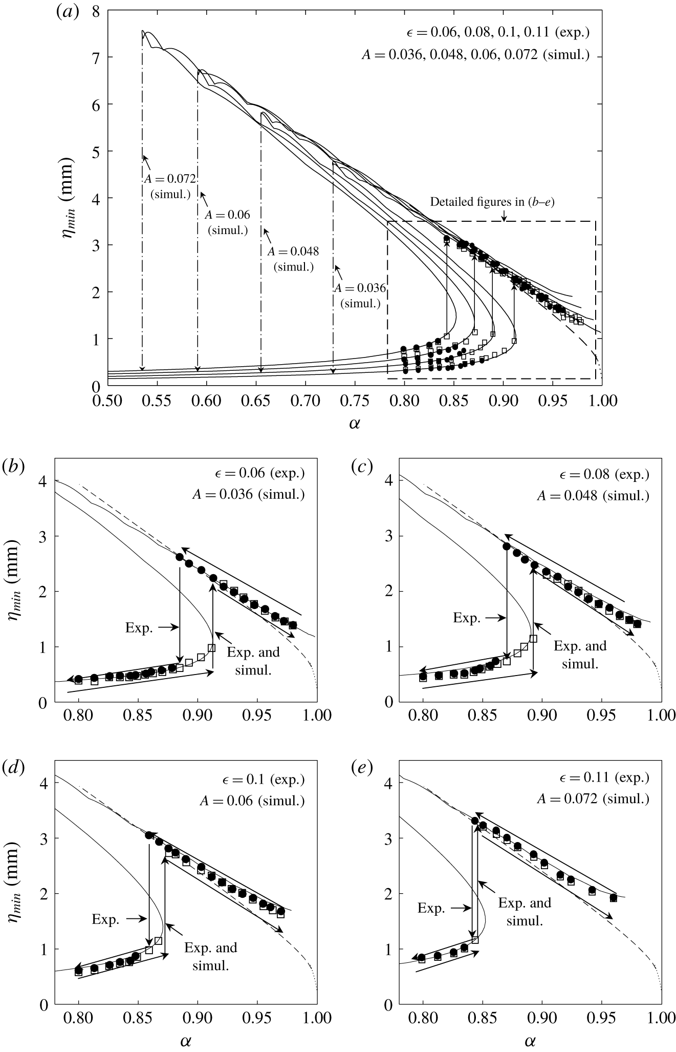
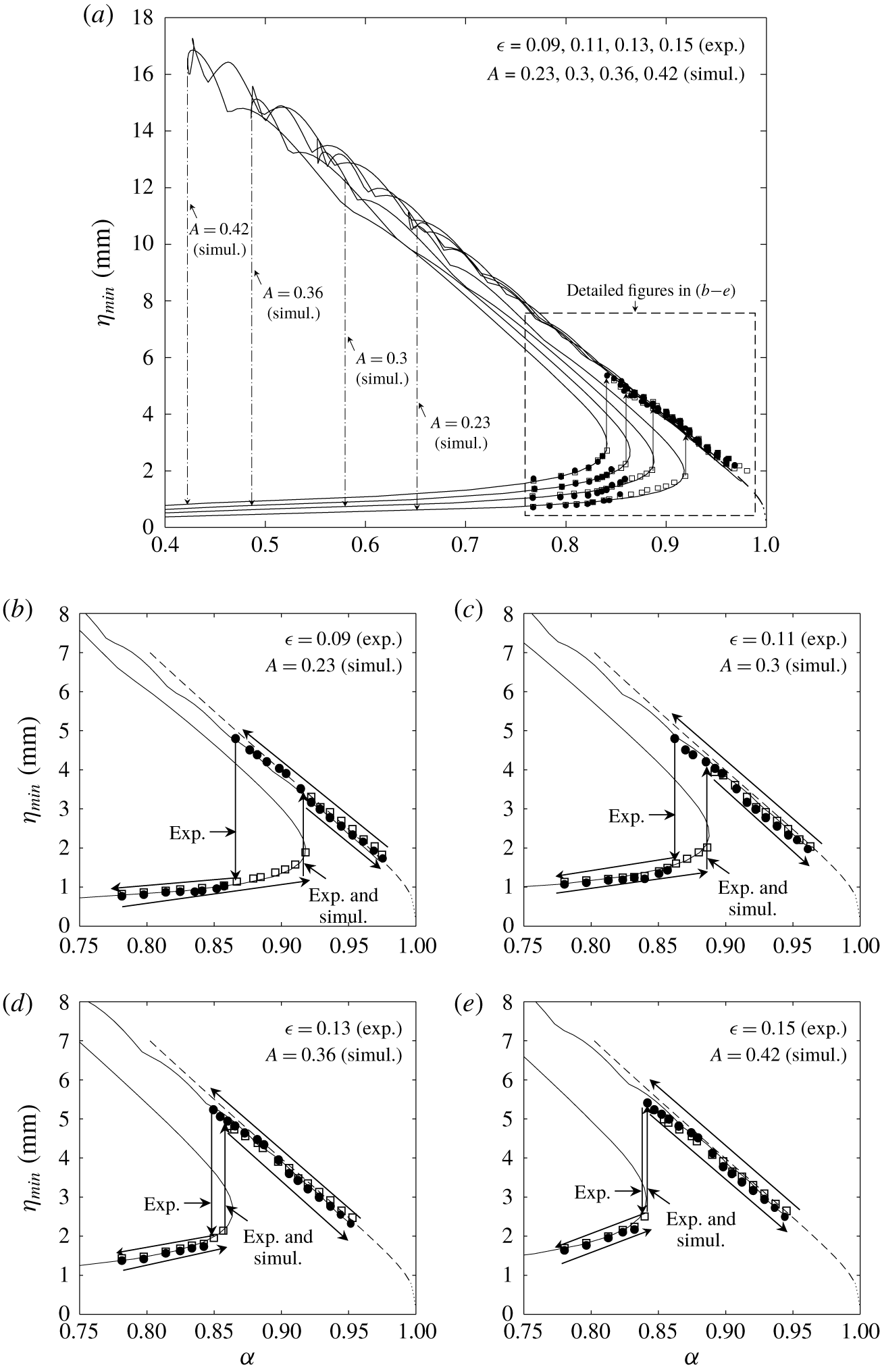
 $\unicode[STIX]{x1D702}$ as unknowns (Cho et al. Reference Cho, Diorio, Akylas and Duncan2011; Cho Reference Cho2014, Reference Cho2018), and the resultant response diagrams are shown in figures 15 and 16 as solid curves. In the figures, the experimental results from figures 8(a) and 8(c) (for 2-D and 3-D air-blowing cases, respectively) are also shown. From these curves, one can understand how those 2-D/3-D gravity–capillary solitary waves with
 $\unicode[STIX]{x1D6FC}_{final}=0.89$ (2-D) and 0.87 (3-D) can be generated from the intermediate initial state-II waves at
 $\unicode[STIX]{x1D6FC}_{initial,2}=0.96$. The critical speeds (
 $\unicode[STIX]{x1D6FC}_{crit}$) found in the experiments are exactly the first turning point in the response diagrams. As already described in the previous section, these steeper 2-D/3-D gravity–capillary solitary waves cannot be experimentally observed for forcing speeds far below the critical speed (
 $\unicode[STIX]{x1D6FC}_{crit}$) and, below a certain forcing speed (
 $\unicode[STIX]{x1D6FC}_{crit,2}$), small-amplitude linear 2-D/3-D localized waves are observed instead, i.e. a jump transition from nonlinear to linear states. For example, starting from the state-II initial conditions with
 $\unicode[STIX]{x1D6FC}_{initial,2}=0.96$, in the experiment, the jump transition occurs at
 $\unicode[STIX]{x1D6FC}_{final}=\unicode[STIX]{x1D6FC}_{crit,2}=0.89$ (2-D blowing case:
 $\unicode[STIX]{x1D716}=0.06$) and
 $\unicode[STIX]{x1D6FC}_{final}=\unicode[STIX]{x1D6FC}_{crit,2}=0.87$ (3-D blowing case:
 $\unicode[STIX]{x1D716}=0.09$), respectively (figures 15b and 16b). In the simulation, however, the jump transition occurs at
 $\unicode[STIX]{x1D6FC}_{final}=\unicode[STIX]{x1D6FC}_{crit,2}=0.72$ (2-D blowing case:
 $A=0.036$) and
 $\unicode[STIX]{x1D6FC}_{final}=\unicode[STIX]{x1D6FC}_{crit,2}=0.65$ (3-D blowing case:
 $A=0.23$), respectively, which are the second turning points in the theoretical response diagrams (figures 15a and 16a). We suspect that this discrepancy may come from the imperfect smoothness of the deceleration process in the experiments, which is not a problem in the simulation of the model equation. For different 2-D/3-D air-blowing forcing magnitudes with
 $\unicode[STIX]{x0394}t=7$ s, similar experimental and simulation results are obtained, as shown in figures 15 and 16. In appendix C, experimental results for 2-D/3-D air-suction cases are also shown for different forcing magnitudes (figures 17–25).
Maximum depression of the resultant steady waves versus forcing speed ( $\unicode[STIX]{x1D6FC}$) for different 2-D air-blowing magnitudes. (a) Overall diagram. (b)
 $\unicode[STIX]{x1D716}=0.06$ (Exp.),
 $A=0.036$ (Simul.). (c)
 $\unicode[STIX]{x1D716}=0.08$ (Exp.),
 $A=0.048$ (Simul.). (d)
 $\unicode[STIX]{x1D716}=0.1$ (Exp.),
 $A=0.06$ (Simul.). (e)
 $\unicode[STIX]{x1D716}=0.11$,
 $A=0.072$ (Simul.). Solid curves: solutions to the viscous forced equation (4.5). Dashed curves: solutions to the inviscid forcing-free equations (A 1). For experimental data, the descriptions of symbols (▫ and ●) are the same as those in figure 8.

Maximum depression of the resultant steady waves versus forcing speed ( $\unicode[STIX]{x1D6FC}$) for different 3-D air-blowing magnitudes. (a) Overall diagram. (b)
 $\unicode[STIX]{x1D716}=0.09$ (Exp.),
 $A=0.23$ (Simul.). (c)
 $\unicode[STIX]{x1D716}=0.11$ (Exp.),
 $A=0.3$ (Simul.). (d)
 $\unicode[STIX]{x1D716}=0.13$ (Exp.),
 $A=0.36$ (Simul.). (e)
 $\unicode[STIX]{x1D716}=0.15$,
 $A=0.42$ (Simul.). Solid curves: solutions to the viscous forced equation (4.6). Dashed curves: solutions to the inviscid forcing-free equations (A 2). For experimental data, the descriptions of symbols (▫ and ●) are the same as those in figure 8.

5 Summary
Hysteresis phenomena in forced gravity–capillary waves on deep water where the minimum phase speed  $c_{min}=23~\text{cm}~\text{s}^{-1}$ are experimentally investigated. Four kinds of forcings are considered: 2-D/3-D air-blowing/air-suction forcings. First, for a still-water initial condition, as the forcing speed increases from zero towards a certain target speed (
 $U$), there exists a certain critical speed (
 $U_{crit}$) at which the transition from linear to nonlinear states occurs. When
 $U<U_{crit}$, steady linear localized waves are observed (state I). When
 $U_{crit}<U<c_{min}$, steady nonlinear localized waves, including steep gravity–capillary solitary waves, are observed (state II). When
 $U\approx c_{min}$, periodic shedding phenomena of nonlinear localized depressions are observed (state III). When
 $U>c_{min}$, steady linear non-local waves are observed (state IV). Next, with these state-II, III and IV waves as new initial conditions, as the forcing speed is decreased towards a certain target speed (
 $U_{final}$), a certain critical speed (
 $U_{crit,2}$) is identified at which the transition from nonlinear to linear states occurs. When
 $U_{crit,2}<U_{final}<U_{crit}$, relatively steeper steady nonlinear localized waves, including steeper gravity–capillary solitary waves, are observed. When
 $U_{final}<U_{crit,2}$, state-I waves are observed. These are experimentally observed hysteresis phenomena, which show jump transitions from linear to nonlinear states at a certain critical speed and from nonlinear to linear states at another critical speed, showing the dependence of a state on its history starting from different initial conditions. For 2-D/3-D air-blowing cases, in particular, experimental results are compared with simulation results based on a theoretical model equation. Overall, they agree with each other very well, except that the experimentally identified critical speed (
 $U_{crit,2}$) at which the transition from nonlinear to linear states occurs is different from the theoretically predicted speed, the so-called second turning point in the response diagram. For 2-D/3-D air-suction cases, only experimental results are shown. Further study will be needed to derive a model equation that can explain the suction-forcing experimental results reasonably well and this is left as future work.
Acknowledgement
This work was supported by the National Research Foundation of Korea (NRF) (NRF-2017R1D1A1B03028299).
Declaration of interests
The authors report no conflict of interest.
Appendix A. Steady 2-D/3-D inviscid forcing-free equation for gravity–capillary waves
The model equations whose solutions are the 2-D/3-D inviscid forcing-free gravity–capillary solitary waves are as follows (Cho et al. Reference Cho, Diorio, Akylas and Duncan2011; Park & Cho Reference Park and Cho2016; Cho Reference Cho2018; Park & Cho Reference Park and Cho2018):
 $$\begin{eqnarray}\displaystyle & \displaystyle \unicode[STIX]{x1D6FC}\unicode[STIX]{x1D702}_{x}-{\textstyle \frac{1}{2}}\unicode[STIX]{x1D702}_{x}-{\textstyle \frac{1}{4}}\mathscr{H}\{\unicode[STIX]{x1D702}_{xx}-\unicode[STIX]{x1D702}\}-\unicode[STIX]{x1D6FD}(\unicode[STIX]{x1D702}^{2})_{x}=0,\quad (\text{2-D}), & \displaystyle\end{eqnarray}$$
 $$\begin{eqnarray}\displaystyle & \displaystyle \underbrace{\unicode[STIX]{x1D6FC}\unicode[STIX]{x1D702}_{x}}_{convection}\underbrace{-{\textstyle \frac{1}{2}}\unicode[STIX]{x1D702}_{x}-{\textstyle \frac{1}{4}}\mathscr{H}\{\unicode[STIX]{x1D702}_{xx}+2\unicode[STIX]{x1D702}_{yy}-\unicode[STIX]{x1D702}\}}_{dispersion}\underbrace{-\unicode[STIX]{x1D6FD}(\unicode[STIX]{x1D702}^{2})_{x}}_{nonlinear\,steepening}=0,\quad (\text{3-D}), & \displaystyle\end{eqnarray}$$
where  $\unicode[STIX]{x1D702}(x)$ and
 $\unicode[STIX]{x1D702}(x,y)$ are dimensionless wave solutions in (A 1) and (A 2), respectively,
 $x$ is the dimensionless coordinate in the moving frame with speed
 $\unicode[STIX]{x1D6FC}$,
 $y$ is the dimensionless transverse coordinate to the coordinate
 $x$, the nonlinear coefficient is
 $\unicode[STIX]{x1D6FD}=(\sqrt{11/2})/8$, the subscript indicates partial differentiation and
 $\mathscr{H}$ denotes the following Hilbert transform:
 $$\begin{eqnarray}\displaystyle & \displaystyle \mathscr{H}(f)=\mathscr{F}^{-1}\{-\text{i}\,\text{sign}(k)\mathscr{F}(f)\}, & \displaystyle\end{eqnarray}$$
 $$\begin{eqnarray}\displaystyle & \displaystyle \mathscr{F}(f)=\int _{-\infty }^{\infty }f(x,y)\text{e}^{-\text{i}kx}\,\text{d}x,\quad (\text{2-D}), & \displaystyle\end{eqnarray}$$
 $$\begin{eqnarray}\displaystyle & \displaystyle \mathscr{F}(f)=\int _{-\infty }^{\infty }\int _{-\infty }^{\infty }f(x,y)\text{e}^{-\text{i}kx-\text{i}ly}\,\text{d}x\,\text{d}y,\quad (\text{3-D}), & \displaystyle\end{eqnarray}$$
where  $k$ and
 $l$ are wavenumbers in the
 $x$ and
 $y$ directions, respectively. For 2-D and 3-D inviscid forcing-free gravity–capillary solitary waves, (A 1), (A 3) and (A 4) and (A 2), and (A 3) and (A 5) are solved, respectively, using the modified Petviashvili method (Cho Reference Cho2015). For a dimensional result, the characteristic length
 $L=(\unicode[STIX]{x1D70E}/\unicode[STIX]{x1D70C}g)^{1/2}=2.73~\text{mm}$ will be multiplied to dimensionless results, where
 $\unicode[STIX]{x1D70E}$ is the surface tension,
 $\unicode[STIX]{x1D70C}$ is the water density and
 $g$ is the gravitational acceleration. In the derivation of model equations, rather than using only quadratic nonlinearity, we can adopt both quadratic and cubic nonlinearities as shown in appendix B. However, the overall result changes little regardless of the added complication (Cho Reference Cho2010).
Appendix B. Quadratic and cubic nonlinearities
In the derivation of model equations, we can adopt both quadratic and cubic nonlinearities with coefficients  $\unicode[STIX]{x1D6FD}$ and
 $\unicode[STIX]{x1D6FF}$, respectively, as follows:
 $$\begin{eqnarray}\unicode[STIX]{x1D6FC}\unicode[STIX]{x1D702}_{x}-{\textstyle \frac{1}{2}}\unicode[STIX]{x1D702}_{x}-{\textstyle \frac{1}{4}}\mathscr{H}\{\unicode[STIX]{x1D702}_{xx}+2\unicode[STIX]{x1D702}_{yy}-\unicode[STIX]{x1D702}\}-\unicode[STIX]{x1D6FD}(\unicode[STIX]{x1D702}^{2})_{x}-\unicode[STIX]{x1D6FF}(\unicode[STIX]{x1D702}^{3})_{x}=0.\end{eqnarray}$$
In the small-amplitude limit near  $\unicode[STIX]{x1D6FC}=1$, the solution of (B 1) can be expanded as
 $$\begin{eqnarray}\unicode[STIX]{x1D702}={\textstyle \frac{1}{2}}\unicode[STIX]{x1D716}\{S(X,Y)\text{e}^{\text{i}x}+\text{c.c.}\}+{\textstyle \frac{1}{2}}\unicode[STIX]{x1D716}^{2}\{S_{2}(X,Y)\text{e}^{2\text{i}x}+\text{c.c.}\}+\cdots \,.\end{eqnarray}$$
As a result, the associated nonlinear Schrödinger equation for  $S$ is governed by
 $$\begin{eqnarray}-S+{\textstyle \frac{1}{4}}(S_{XX}+2S_{YY})+{\textstyle \frac{1}{4}}(16\unicode[STIX]{x1D6FD}^{2}-3\unicode[STIX]{x1D6FF})S^{2}S^{\ast }=0.\end{eqnarray}$$
In addition, the relation between  $S$ and
 $S_{2}$ is
 $$\begin{eqnarray}S_{2}=-4\unicode[STIX]{x1D6FD}S^{2}.\end{eqnarray}$$
On the other hand, if the expansion (B 2) is used in the full-water wave equations, we find the following two equations which correspond to (B 3) and (B 4), respectively:
 $$\begin{eqnarray}\displaystyle & \displaystyle -S+{\textstyle \frac{1}{4}}(S_{XX}+2S_{YY})+{\textstyle \frac{11}{32}}S^{2}S^{\ast }=0, & \displaystyle\end{eqnarray}$$
 $$\begin{eqnarray}\displaystyle & \displaystyle S_{2}=-S^{2}. & \displaystyle\end{eqnarray}$$
From (B 3)–(B 6), by comparison, the coefficients of quadratic and cubic nonlinearities are found to be  $\unicode[STIX]{x1D6FD}=1/4$ and
 $\unicode[STIX]{x1D6FF}=-1/8$.
Appendix C
Side-view wave profiles according to the variation of 2-D air-suction forcing ( $\unicode[STIX]{x1D6FE}=0.04$) speed (
 $\unicode[STIX]{x1D6FC}_{initial,1}=0~(t=0~\text{s})\rightarrow \unicode[STIX]{x1D6FC}_{initial,2}~(t=0.6{-}3~\text{s})\rightarrow \unicode[STIX]{x1D6FC}_{final}~(t=10{-}13~\text{s})$) where the intermediate initial condition is the state-II wave at
 $\unicode[STIX]{x1D6FC}_{initial,2}=0.96$.

Side-view wave profiles according to the variation of 2-D air-suction forcing ( $\unicode[STIX]{x1D6FE}=0.04$) speed (
 $\unicode[STIX]{x1D6FC}_{initial,1}=0~(t=0~\text{s})\rightarrow \unicode[STIX]{x1D6FC}_{initial,2}~(t=0.6{-}3~\text{s})\rightarrow \unicode[STIX]{x1D6FC}_{final}~(t=10{-}13~\text{s})$) where the intermediate initial condition is the state-III wave at
 $\unicode[STIX]{x1D6FC}_{initial,2}=1$.

Side-view wave profiles according to the variation of 2-D air-suction forcing ( $\unicode[STIX]{x1D6FE}=0.04$) speed (
 $\unicode[STIX]{x1D6FC}_{initial,1}=0~(t=0~\text{s})\rightarrow \unicode[STIX]{x1D6FC}_{initial,2}~(t=0.6{-}3~\text{s})\rightarrow \unicode[STIX]{x1D6FC}_{final}~(t=10{-}13~\text{s})$) where the intermediate initial condition is the state-IV wave at
 $\unicode[STIX]{x1D6FC}_{initial,2}=1.1$.

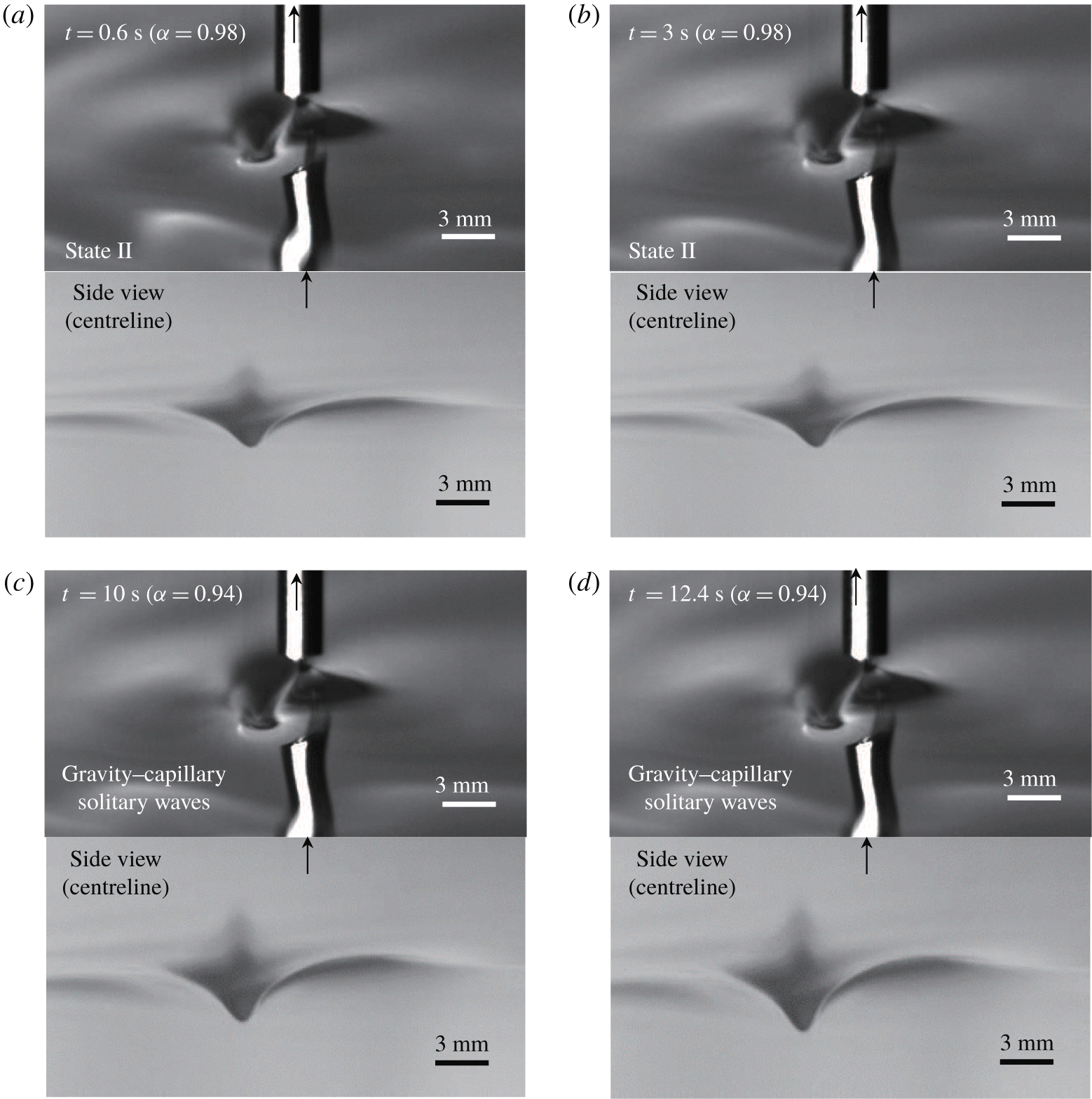
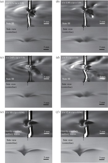
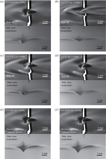
Wave profiles according to the variation of 3-D air-suction forcing ( $\unicode[STIX]{x1D6FE}=0.04$) speed (
 $\unicode[STIX]{x1D6FC}_{initial,1}=0~(t=0~\text{s})\rightarrow \unicode[STIX]{x1D6FC}_{initial,2}~(t=0.6{-}3~\text{s})\rightarrow \unicode[STIX]{x1D6FC}_{final}~(t=10{-}13~\text{s})$) where the intermediate initial condition is the state-II wave at
 $\unicode[STIX]{x1D6FC}_{initial,2}=0.98$. Upper pictures: experimental results (3-D view). Lower pictures: experimental results (side view).

Wave profiles according to the variation of 3-D air-suction forcing ( $\unicode[STIX]{x1D6FE}=0.04$) speed (
 $\unicode[STIX]{x1D6FC}_{initial,1}=0~(t=0~\text{s})\rightarrow \unicode[STIX]{x1D6FC}_{initial,2}~(t=0.6{-}3~\text{s})\rightarrow \unicode[STIX]{x1D6FC}_{final}~(t=10{-}13~\text{s})$) where the intermediate initial condition is the state-III wave at
 $\unicode[STIX]{x1D6FC}_{initial,2}=1$. Upper pictures: experimental results (3-D view). Lower pictures: experimental results (side view).

Wave profiles according to the variation of 3-D air-suction forcing ( $\unicode[STIX]{x1D6FE}=0.04$) speed (
 $\unicode[STIX]{x1D6FC}_{initial,1}=0~(t=0~\text{s})\rightarrow \unicode[STIX]{x1D6FC}_{initial,2}~(t=0.6{-}3~\text{s})\rightarrow \unicode[STIX]{x1D6FC}_{final}~(t=10{-}13~\text{s})$) where the intermediate initial condition is the state-III wave at
 $\unicode[STIX]{x1D6FC}_{initial,2}=0.99$ (‘snap-stick’ phenomena). Upper pictures: experimental results (3-D view). Lower pictures: experimental results (side view).

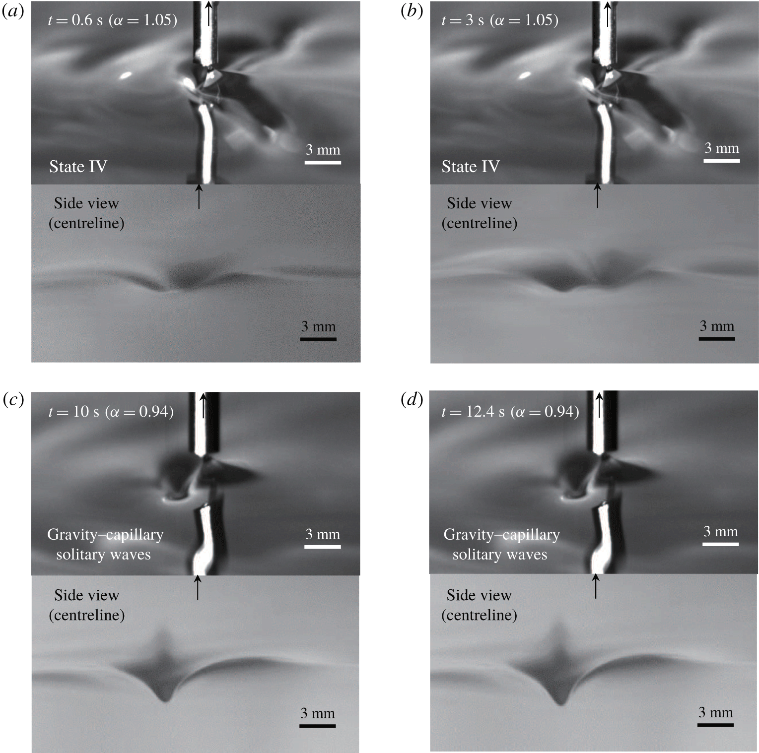
Wave profiles according to the variation of 3-D air-suction forcing ( $\unicode[STIX]{x1D6FE}=0.04$) speed (
 $\unicode[STIX]{x1D6FC}_{initial,1}=0~(t=0~\text{s})\rightarrow \unicode[STIX]{x1D6FC}_{initial,2}~(t=0.6{-}3~\text{s})\rightarrow \unicode[STIX]{x1D6FC}_{final}~(t=10{-}13~\text{s})$) where the intermediate initial condition is the state-IV wave at
 $\unicode[STIX]{x1D6FC}_{initial,2}=1.05$. Upper pictures: experimental results (3-D view). Lower pictures: experimental results (side view).

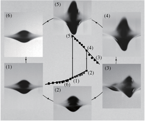
Maximum depression of the resultant steady waves versus forcing speed ( $\unicode[STIX]{x1D6FC}$) for different 2-D air-suction magnitudes. (a)
 $\unicode[STIX]{x1D6FE}=0.04$. (b)
 $\unicode[STIX]{x1D6FE}=0.07$. (c)
 $\unicode[STIX]{x1D6FE}=0.1$. (d)
 $\unicode[STIX]{x1D6FE}=0.12$. Dashed curves: solutions to the inviscid forcing-free equations (A 1). Descriptions of symbols (▫ and ●) are the same as those in figure 8.

Maximum depression of the resultant steady waves versus forcing speed ( $\unicode[STIX]{x1D6FC}$) for different 3-D air-suction magnitudes. (a)
 $\unicode[STIX]{x1D6FE}=0.04$. (b)
 $\unicode[STIX]{x1D6FE}=0.07$. (c)
 $\unicode[STIX]{x1D6FE}=0.1$. (d)
 $\unicode[STIX]{x1D6FE}=0.14$. Dashed curves: solutions to the inviscid forcing-free equations (A 2). Descriptions of symbols (▫ and ●) are the same as those in figure 8.