1 Introduction
Buoyancy-driven flow in porous media is well established both as a source of rich fluid dynamics and as a topic of practical and scientific interest, with areas of application including geothermal reservoirs, carbon sequestration, ore emplacement, and oil and gas extraction. It is becoming increasingly appreciated that in many geological settings such flow is coupled to geochemical processes and that these processes in turn can influence the flow both by altering the buoyancy of the fluid and by changing the structure of the porous rock (Phillips Reference Phillips2009). Analogies can be drawn between these dynamics and those of mushy layers (Worster Reference Worster1997), although the dominant thermodynamical processes in the latter case are rather different.
Two paradigm problems for buoyancy-driven flow in porous media are well established: the classic Horton–Rogers–Lapwood (HRL) problem (Horton & Rogers Reference Horton and Rogers1945; Lapwood Reference Lapwood1948) of convection driven by an imposed buoyancy gradient and the problem of a buoyantly unstable boundary layer (BUBL) caused, for example, by the introduction of relatively dense fluid near the upper boundary of the domain (see Riaz et al. (Reference Riaz, Hesse, Tchelepi and Orr2006), and references therein). Meanwhile, the classic problem in flow–permeability feedback is the wormholing instability which develops as, for example, a front of undersaturated or acidised fluid invades a partially soluble or reactive porous medium. (Szymczak & Ladd (Reference Szymczak and Ladd2014) provide a comprehensive account of this instability.) This instability is of particular importance to acidising treatments of carbonate reservoirs, both during matrix acidisation (Panga, Ziauddin & Balakotaiah Reference Panga, Ziauddin and Balakotaiah2005), when it creates high-permeability channels in the matrix, and during acid fracturing, when it may influence channel etching (Mou, Zhu & Hill Reference Mou, Zhu and Hill2010) and acid leakoff (Zhang et al. Reference Zhang, Yang, Zhang and Mou2014). In these contexts, the flow is principally driven by the pressure gradients associated with injection and so buoyancy is unimportant. However, flow–permeability feedback is also known to occur during convection in magmatic and hydrothermal systems (Bolton, Lasaga & Rye Reference Bolton, Lasaga and Rye1996, Reference Bolton, Lasaga and Rye1997, Reference Bolton, Lasaga and Rye1999; Weis Reference Weis2015), and during vertical flow in karst formations (Petrus & Szymczak Reference Petrus and Szymczak2016).
Much attention has been given in recent years to variations on the BUBL problem, motivated by the process of solution trapping in geological CO
 $_{2}$
sequestration (Huppert & Neufeld Reference Huppert and Neufeld2014; Celia et al.
Reference Celia, Bachu, Nordbotten and Bandilla2015). In this process, relatively buoyant liquid CO
 $_{2}$
is introduced near the top of a brine-filled saline aquifer. As the CO
 $_{2}$
and brine mix diffusively, they produce a solution that is denser than either, causing a buoyant instability which acts to mix the CO
 $_{2}$
more thoroughly through the aquifer. Several recent studies (e.g. Andres & Cardoso Reference Andres and Cardoso2011; Ward et al.
Reference Ward, Cliffe, Jensen and Power2014a
,Reference Ward, Jensen, Power and Riley
b
; Hidalgo et al.
Reference Hidalgo, Dentz, Cabeza and Carrera2015; Cherezov & Cardoso Reference Cherezov and Cardoso2016; Barba Rossa, Cliffe & Power Reference Barba Rossa, Cliffe and Power2017; Ghoshal, Kim & Cardoso Reference Ghoshal, Kim and Cardoso2017) have modelled this process, representing the dissolution of CO
 $_{2}$
or its interaction with the porous matrix as ‘reaction’ terms in the solute transport equation; recent experimental work by Vreme et al. (Reference Vreme, Nadal, Pouligny, Jeandet, Liger-Belair and Meunier2016) and Ching, Chen & Tsai (Reference Ching, Chen and Tsai2017) complements this modelling. A particularly interesting study of this kind is the work of Ward et al. (Reference Ward, Jensen, Power and Riley2015), who investigated the process by which the BUBL can degrade the porous substrate by dissolving one of the minerals that constitute it. Meanwhile, the recent contribution by Petrus & Szymczak (Reference Petrus and Szymczak2016) has investigated the development of vertical pipes through the dissolution of a layered porous medium by vertically percolating water.
The HRL problem with reactive or dissolutional effects has received less attention, but remains a valuable testbed on which to explore the complex interactions between these effects and buoyant flow. This problem was first investigated by Steinberg & Brand (Reference Steinberg and Brand1983, Reference Steinberg and Brand1984), with subsequent contributions by Gatica, Viljoen & Hlavacek (Reference Gatica, Viljoen and Hlavacek1989) and Viljoen, Gatica & Hlavacek (Reference Viljoen, Gatica and Hlavacek1990). Pritchard & Richardson (Reference Pritchard and Richardson2007) built on this work by investigating the onset of double-diffusive convection, in which the equilibrium solute concentration depends on the local temperature, leading to the precipitation or dissolution of solute as the temperature of a fluid element changes. Their model has since been extended in various ways; the contribution of Malashetty & Biradar (Reference Malashetty and Biradar2011), who investigated the effect of anisotropy, is perhaps the most significant.
So far, very little work on the HRL problem has directly considered the feedback between the exchange of a mineral with the porous matrix, the consequent changes to porosity and permeability, and the large-scale flow patterns that result. In complex geological settings, such effects have been investigated through numerical simulations (e.g. Bolton et al. Reference Bolton, Lasaga and Rye1996, Reference Bolton, Lasaga and Rye1997, Reference Bolton, Lasaga and Rye1999; Weis Reference Weis2015), but more fundamental studies have been scarce. Ritchie & Pritchard (Reference Ritchie and Pritchard2011) considered a simplified version of Pritchard & Richardson’s (Reference Pritchard and Richardson2007) problem, in which the temperature field was treated as independent of the flow, so that a constant gradient of temperature and thus of equilibrium solubility was maintained. The interaction between flow and permeability evolution proved to be rather intricate, with a novel reaction–diffusion mechanism emerging at low Rayleigh numbers; over longer time scales, flow–permeability feedback was found to trigger secondary instabilities and ultimately to create characteristic patterns of porosity, including both horizontal layering and vertical high-porosity chimneys.
The present study builds directly on the work of Pritchard & Richardson (Reference Pritchard and Richardson2007) and Ritchie & Pritchard (Reference Ritchie and Pritchard2011). Rather than simplifying the treatment of the temperature field, we consider full double-diffusive convection with evolving permeability. We pay particular attention to the regime in which the temperature gradient is destabilising, in which we find that the interaction between flow and permeability creates an inhomogeneous pattern of porosity that is substantially different from that found by Ritchie & Pritchard (Reference Ritchie and Pritchard2011).
The remainder of the paper is organised as follows. In § 2 we present a model of double-diffusive convection in a porous medium with evolving porosity. In § 3, we carry out a linear stability analysis of the onset of convection. In § 4, we carry out numerical simulations to investigate the longer-term behaviour of the system. Finally, in § 5, we summarise our results and draw some general conclusions.
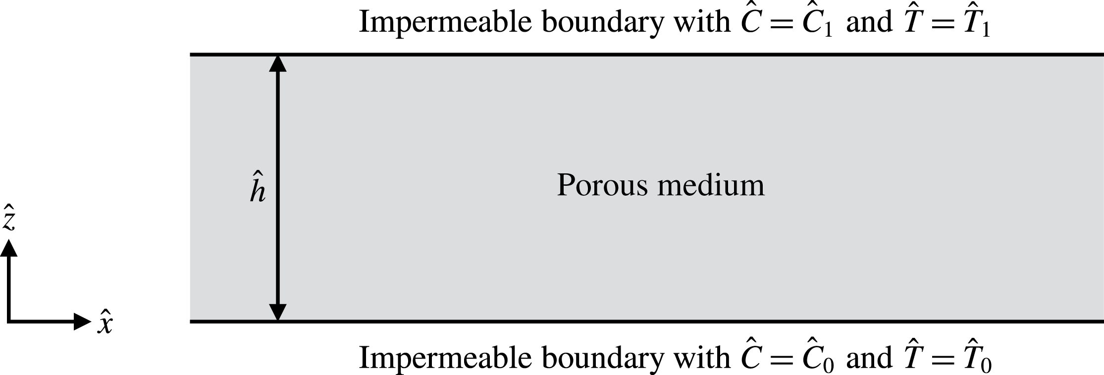
Sketch of the geometry of the problem: an initially homogeneous and isotropic porous layer of depth
 ${\hat{h}}$
with impermeable boundaries at the top and the bottom.

2 Model description
We consider two-dimensional flow in an initially homogeneous and isotropic porous layer of depth
 ${\hat{h}}$
with solutal mass concentrations
 ${\hat{C}}_{0}$
and
 ${\hat{C}}_{1}$
and temperatures
 $\hat{T}_{0}$
and
 $\hat{T}_{1}$
imposed at the bottom and top respectively (figure 1). The bottom and top boundaries are impermeable, and we assume chemical equilibrium at the boundaries.
We take
 $\hat{x}$
and
 $\hat{z}$
as the horizontal and vertical coordinates respectively, with
 $\hat{z}$
increasing upwards. Making a Boussinesq approximation, the flow is governed by the equations of mass conservation and Darcy’s law,
 $$\begin{eqnarray}\displaystyle & \displaystyle \frac{\unicode[STIX]{x2202}\unicode[STIX]{x1D719}}{\unicode[STIX]{x2202}\hat{t}}+\hat{\unicode[STIX]{x1D735}}\boldsymbol{\cdot }\hat{\boldsymbol{u}}=0, & \displaystyle\end{eqnarray}$$
 $$\begin{eqnarray}\displaystyle & \displaystyle \hat{\boldsymbol{u}}=-\frac{\hat{K}(\unicode[STIX]{x1D719})}{\hat{\unicode[STIX]{x1D707}}}\hat{\unicode[STIX]{x1D735}}\hat{p}-\frac{\hat{K}(\unicode[STIX]{x1D719})}{\hat{\unicode[STIX]{x1D707}}}\hat{\unicode[STIX]{x1D70C}}_{\text{f}}({\hat{C}},\hat{T}){\hat{g}}\boldsymbol{e}_{z}, & \displaystyle\end{eqnarray}$$
where
 $\hat{K}(\unicode[STIX]{x1D719})$
is the permeability, which depends on the porosity
 $\unicode[STIX]{x1D719}$
,
 $\hat{\unicode[STIX]{x1D707}}$
is the fluid viscosity,
 $\hat{\unicode[STIX]{x1D70C}}_{\text{f}}$
is the fluid density, which depends on the mass concentration of solute in the fluid
 ${\hat{C}}$
and the temperature
 $\hat{T}$
, and
 $\hat{\boldsymbol{u}}=(\hat{u} ,{\hat{w}})$
is the transport velocity. A caret denotes a dimensional variable, while dimensionless variables are unadorned.
Following Phillips (Reference Phillips2009, § 5.5), the permeability
 $\hat{K}(\unicode[STIX]{x1D719})$
is given by
 $$\begin{eqnarray}\displaystyle \hat{K}(\unicode[STIX]{x1D719})=\hat{K}_{0}\left(\frac{\unicode[STIX]{x1D719}}{\unicode[STIX]{x1D719}_{0}}\right)^{b}, & & \displaystyle\end{eqnarray}$$
where
 $\hat{K}_{0}$
and
 $\unicode[STIX]{x1D719}_{0}$
are the initial permeability and porosity respectively. The exponent
 $b$
typically lies between 2 and 3 inclusive. We will take
 $b=2$
throughout.
Assuming local thermal equilibrium, the transport of heat and solute is described by the advection–diffusion equations
 $$\begin{eqnarray}\displaystyle & \displaystyle (\hat{\unicode[STIX]{x1D70C}}{\hat{c}})_{\text{m}}\frac{\unicode[STIX]{x2202}\hat{T}}{\unicode[STIX]{x2202}\hat{t}}+(\hat{\unicode[STIX]{x1D70C}}{\hat{c}})_{\text{f}}(\hat{\boldsymbol{u}}\boldsymbol{\cdot }\hat{\unicode[STIX]{x1D735}})\hat{T}=(\hat{\unicode[STIX]{x1D70C}}{\hat{c}})_{\text{m}}\hat{\unicode[STIX]{x1D705}}_{\text{T}}\hat{\unicode[STIX]{x1D6FB}}^{2}\hat{T}, & \displaystyle\end{eqnarray}$$
 $$\begin{eqnarray}\displaystyle & \displaystyle \frac{\unicode[STIX]{x2202}(\unicode[STIX]{x1D719}{\hat{C}})}{\unicode[STIX]{x2202}\hat{t}}+\hat{\unicode[STIX]{x1D735}}\boldsymbol{\cdot }(\hat{\boldsymbol{u}}{\hat{C}})=\hat{\unicode[STIX]{x1D735}}\boldsymbol{\cdot }(\unicode[STIX]{x1D719}\hat{\unicode[STIX]{x1D705}}_{\text{C}}\hat{\unicode[STIX]{x1D735}}{\hat{C}})+\hat{k}(\unicode[STIX]{x1D719})({\hat{C}}_{\text{eq}}(\hat{T})-{\hat{C}}). & \displaystyle\end{eqnarray}$$
Here,
 ${\hat{C}}_{\text{eq}}(\hat{T})$
is the equilibrium concentration of solute at a given temperature;
 $\hat{\unicode[STIX]{x1D705}}_{\text{T}}$
is the effective diffusivity of heat through the saturated medium and
 $\hat{\unicode[STIX]{x1D705}}_{\text{C}}$
is the molecular diffusivity of the solute through the fluid. The volumetric heat capacity of the fluid is given by
 $(\hat{\unicode[STIX]{x1D70C}}{\hat{c}})_{\text{f}}$
and that of the saturated medium is given by
 $(\hat{\unicode[STIX]{x1D70C}}{\hat{c}})_{\text{m}}=\unicode[STIX]{x1D719}(\hat{\unicode[STIX]{x1D70C}}{\hat{c}})_{\text{f}}+(1-\unicode[STIX]{x1D719})(\hat{\unicode[STIX]{x1D70C}}{\hat{c}})_{\text{s}}$
, where the subscript
 $\text{s}$
denotes properties of the solid rock matrix. The solute transport equation (2.5) may be simplified using (2.1) to
 $$\begin{eqnarray}\displaystyle \unicode[STIX]{x1D719}\frac{\unicode[STIX]{x2202}{\hat{C}}}{\unicode[STIX]{x2202}\hat{t}}+(\hat{\boldsymbol{u}}\boldsymbol{\cdot }\hat{\unicode[STIX]{x1D735}}){\hat{C}}=\hat{\unicode[STIX]{x1D705}}_{\text{C}}\hat{\unicode[STIX]{x1D735}}\boldsymbol{\cdot }(\unicode[STIX]{x1D719}\hat{\unicode[STIX]{x1D735}}{\hat{C}})+\hat{k}(\unicode[STIX]{x1D719})({\hat{C}}_{\text{eq}}(\hat{T})-{\hat{C}}). & & \displaystyle\end{eqnarray}$$
The parameter
 $\hat{k}(\unicode[STIX]{x1D719})\geqslant 0$
, which controls the rate of mass exchange between the fluid and the porous matrix due to dissolution and precipitation, implicitly depends on the surface area of the rock exposed to the fluid within the pore network. A variety of models have been used in various contexts to relate such parameters to porosity (e.g. Chadam et al.
Reference Chadam, Ortoleva, Qin and Stamicar2001; Zhao et al.
Reference Zhao, Hobbs, Ord, Hornby and Peng2008; Ward et al.
Reference Ward, Jensen, Power and Riley2015; Petrus & Szymczak Reference Petrus and Szymczak2016). We choose to follow Ritchie & Pritchard (Reference Ritchie and Pritchard2011) and employ the minimal assumption that the rate of mass exchange between the rock and the pore fluid should reduce to zero when either there is no rock or there are no pores. Therefore, we define
 $$\begin{eqnarray}\displaystyle \hat{k}(\unicode[STIX]{x1D719})=\hat{k}_{0}\frac{\unicode[STIX]{x1D719}(1-\unicode[STIX]{x1D719})}{\unicode[STIX]{x1D719}_{0}(1-\unicode[STIX]{x1D719}_{0})}, & & \displaystyle\end{eqnarray}$$
where
 $\hat{k}_{0}$
is the constant initial rate and
 $\unicode[STIX]{x1D719}_{0}$
is the initial porosity. With this definition, we assume that the porous medium consists entirely of soluble species. In realistic geological settings, this assumption is unlikely to hold. However, it provides a reasonable starting point for exploring the effect of porosity evolution on convection.
By mass conservation, the porosity evolution is governed by
 $$\begin{eqnarray}\displaystyle \frac{\unicode[STIX]{x2202}\unicode[STIX]{x1D719}}{\unicode[STIX]{x2202}\hat{t}}=\frac{\hat{k}(\unicode[STIX]{x1D719})}{\hat{\unicode[STIX]{x1D70C}}_{\text{s}}}({\hat{C}}_{\text{eq}}(\hat{T})-{\hat{C}}), & & \displaystyle\end{eqnarray}$$
where
 $\hat{\unicode[STIX]{x1D70C}}_{\text{s}}$
is the solid matrix density.
Finally, we take the density to be given by the linear approximation
 $$\begin{eqnarray}\displaystyle \hat{\unicode[STIX]{x1D70C}}_{\text{f}}({\hat{C}},\hat{T})=\hat{\unicode[STIX]{x1D70C}}_{0}[1+\hat{\unicode[STIX]{x1D6FD}}_{\text{C}}({\hat{C}}-{\hat{C}}_{0})+\hat{\unicode[STIX]{x1D6FD}}_{\text{T}}(\hat{T}-\hat{T}_{0})]. & & \displaystyle\end{eqnarray}$$
Following Pritchard & Richardson (Reference Pritchard and Richardson2007), we take the equilibrium concentration to vary linearly in
 $\hat{T}$
and write
 $$\begin{eqnarray}\displaystyle {\hat{C}}_{\text{eq}}(\hat{T})={\hat{C}}_{0}+\hat{\unicode[STIX]{x1D6FE}}(\hat{T}-\hat{T}_{0}). & & \displaystyle\end{eqnarray}$$
The assumption of chemical equilibrium on the boundaries gives
 $$\begin{eqnarray}\displaystyle \hat{\unicode[STIX]{x1D6FE}}=\frac{{\hat{C}}_{1}-{\hat{C}}_{0}}{\hat{T}_{1}-\hat{T}_{0}}, & & \displaystyle\end{eqnarray}$$
which may be positive or negative. If
 $\hat{\unicode[STIX]{x1D6FE}}>0$
, then the gradients of concentration and temperature must have the same sign, and therefore contribute in opposing senses to the stability, while if
 $\hat{\unicode[STIX]{x1D6FE}}<0$
, then the gradients of concentration and temperature must be of opposite sign, and are therefore either both stabilising or both destabilising (see Pritchard & Richardson (Reference Pritchard and Richardson2007) and references therein for further discussion).
We seek an initial steady-state solution in which
 $\hat{\boldsymbol{u}}=\mathbf{0}$
and there is no lateral variation. We then find a linear distribution of temperature and solute concentration,
 $$\begin{eqnarray}\displaystyle \hat{T}_{\text{b}}(\hat{z})=\hat{T}_{0}+(\hat{T}_{1}-\hat{T}_{0})\frac{\hat{z}}{{\hat{h}}},\quad {\hat{C}}_{\text{b}}(\hat{z})={\hat{C}}_{0}+({\hat{C}}_{1}-{\hat{C}}_{0})\frac{\hat{z}}{{\hat{h}}}. & & \displaystyle\end{eqnarray}$$
The initial distribution of solute corresponds to
 ${\hat{C}}_{\text{b}}={\hat{C}}_{\text{eq}}(\hat{T_{\text{b}}})$
. As noted by Pritchard & Richardson (Reference Pritchard and Richardson2007), taking
 ${\hat{C}}_{\text{eq}}$
to be linear in
 $\hat{T}$
permits the existence of a steady base state in which the solution is at saturation everywhere and so the vertical flux of solute is constant in space.
2.1 Streamfunction formulation and non-dimensionalisation
Under the assumption that the rate of change of porosity is much slower than the transport of dissolved solute, (2.1) may be approximated as
 $$\begin{eqnarray}\displaystyle \hat{\unicode[STIX]{x1D735}}\boldsymbol{\cdot }\hat{\boldsymbol{u}}=0. & & \displaystyle\end{eqnarray}$$
This is a standard simplification (see Ritchie & Pritchard (Reference Ritchie and Pritchard2011) and references therein), which allows us to define a streamfunction
 $\hat{\unicode[STIX]{x1D713}}(\hat{x},\hat{z},\hat{t})$
so that
 $\hat{u} =-\unicode[STIX]{x2202}\hat{\unicode[STIX]{x1D713}}/\unicode[STIX]{x2202}\hat{z}$
and
 ${\hat{w}}=\unicode[STIX]{x2202}\hat{\unicode[STIX]{x1D713}}/\unicode[STIX]{x2202}\hat{x}$
.
We now define dimensionless variables as
 $$\begin{eqnarray}\displaystyle \left.\begin{array}{@{}c@{}}\displaystyle \hat{\boldsymbol{x}}={\hat{h}}\boldsymbol{x},\quad \hat{\unicode[STIX]{x1D713}}=\unicode[STIX]{x1D719}_{0}\hat{\unicode[STIX]{x1D705}}_{\text{T}}\unicode[STIX]{x1D713},\quad \hat{t}=\frac{{\hat{h}}^{2}}{\hat{\unicode[STIX]{x1D705}}_{\text{T}}}t,\\ \displaystyle {\hat{C}}={\hat{C}}_{\text{b}}(\hat{z})+({\hat{C}}_{1}-{\hat{C}}_{0})C^{\prime },\quad \hat{T}=\hat{T}_{\text{b}}(\hat{z})+(\hat{T}_{1}-\hat{T}_{0})T^{\prime },\end{array}\right\} & & \displaystyle\end{eqnarray}$$
where
 $T^{\prime }$
and
 $C^{\prime }$
are perturbations to the base-state temperature and concentration fields respectively. We can then eliminate
 $\hat{p}$
to obtain the dimensionless governing equations
 $$\begin{eqnarray}\displaystyle & \displaystyle \unicode[STIX]{x1D735}\boldsymbol{\cdot }\left[\left(\frac{\unicode[STIX]{x1D719}}{\unicode[STIX]{x1D719}_{0}}\right)^{-2}\unicode[STIX]{x1D735}\unicode[STIX]{x1D713}\right]=-{\mathcal{R}}_{C}\frac{\unicode[STIX]{x2202}C^{\prime }}{\unicode[STIX]{x2202}x}-{\mathcal{R}}_{T}\frac{\unicode[STIX]{x2202}T^{\prime }}{\unicode[STIX]{x2202}x}, & \displaystyle\end{eqnarray}$$
 $$\begin{eqnarray}\displaystyle & \displaystyle \frac{\unicode[STIX]{x2202}T^{\prime }}{\unicode[STIX]{x2202}t}-\unicode[STIX]{x1D706}\left[\frac{\unicode[STIX]{x2202}\unicode[STIX]{x1D713}}{\unicode[STIX]{x2202}z}\frac{\unicode[STIX]{x2202}T^{\prime }}{\unicode[STIX]{x2202}x}-\frac{\unicode[STIX]{x2202}\unicode[STIX]{x1D713}}{\unicode[STIX]{x2202}x}\left(1+\frac{\unicode[STIX]{x2202}T^{\prime }}{\unicode[STIX]{x2202}z}\right)\right]=\unicode[STIX]{x1D6FB}^{2}T^{\prime }, & \displaystyle\end{eqnarray}$$
 $$\begin{eqnarray}\displaystyle & & \displaystyle \unicode[STIX]{x1D719}\frac{\unicode[STIX]{x2202}C^{\prime }}{\unicode[STIX]{x2202}t}-\unicode[STIX]{x1D719}_{0}\left[\frac{\unicode[STIX]{x2202}\unicode[STIX]{x1D713}}{\unicode[STIX]{x2202}z}\frac{\unicode[STIX]{x2202}C^{\prime }}{\unicode[STIX]{x2202}x}-\frac{\unicode[STIX]{x2202}\unicode[STIX]{x1D713}}{\unicode[STIX]{x2202}x}\left(1+\frac{\unicode[STIX]{x2202}C^{\prime }}{\unicode[STIX]{x2202}z}\right)\right]\nonumber\\ \displaystyle & & \displaystyle \quad =\frac{1}{Le}\left[\unicode[STIX]{x1D719}~\unicode[STIX]{x1D6FB}^{2}C^{\prime }+\frac{\unicode[STIX]{x2202}\unicode[STIX]{x1D719}}{\unicode[STIX]{x2202}x}\frac{\unicode[STIX]{x2202}C^{\prime }}{\unicode[STIX]{x2202}x}+\frac{\unicode[STIX]{x2202}\unicode[STIX]{x1D719}}{\unicode[STIX]{x2202}z}\left(1+\frac{\unicode[STIX]{x2202}C^{\prime }}{\unicode[STIX]{x2202}z}\right)\right]+k_{0}\frac{\unicode[STIX]{x1D719}(1-\unicode[STIX]{x1D719})}{1-\unicode[STIX]{x1D719}_{0}}(T^{\prime }-C^{\prime }),\end{eqnarray}$$
 $$\begin{eqnarray}\displaystyle \frac{\unicode[STIX]{x2202}\unicode[STIX]{x1D719}}{\unicode[STIX]{x2202}t}=\unicode[STIX]{x1D6FF}k_{0}\frac{\unicode[STIX]{x1D719}(1-\unicode[STIX]{x1D719})}{1-\unicode[STIX]{x1D719}_{0}}(T^{\prime }-C^{\prime }), & & \displaystyle\end{eqnarray}$$
subject to the boundary conditions
 $$\begin{eqnarray}\displaystyle \frac{\unicode[STIX]{x2202}\unicode[STIX]{x1D713}}{\unicode[STIX]{x2202}x}=0,\quad T^{\prime }=0\quad \text{and}\quad C^{\prime }=0\quad \text{at}~z=0~\text{and at}~z=1. & & \displaystyle\end{eqnarray}$$
The dimensionless parameters
 ${\mathcal{R}}_{C}$
,
 ${\mathcal{R}}_{T}$
,
 $Le$
,
 $\unicode[STIX]{x1D706}$
,
 $k_{0}$
and
 $\unicode[STIX]{x1D6FF}$
are defined as
 $$\begin{eqnarray}\displaystyle \left.\begin{array}{@{}c@{}}\displaystyle {\mathcal{R}}_{C}=\frac{\hat{K}_{0}\hat{\unicode[STIX]{x1D70C}}_{0}{\hat{g}}{\hat{h}}\hat{\unicode[STIX]{x1D6FD}}_{\text{C}}({\hat{C}}_{1}-{\hat{C}}_{0})}{\unicode[STIX]{x1D719}_{0}\hat{\unicode[STIX]{x1D707}}\hat{\unicode[STIX]{x1D705}}_{\text{T}}},\quad {\mathcal{R}}_{T}=\frac{\hat{K}_{0}\hat{\unicode[STIX]{x1D70C}}_{0}{\hat{g}}{\hat{h}}\hat{\unicode[STIX]{x1D6FD}}_{\text{T}}(\hat{T}_{1}-\hat{T}_{0})}{\unicode[STIX]{x1D719}_{0}\hat{\unicode[STIX]{x1D707}}\hat{\unicode[STIX]{x1D705}}_{\text{T}}},\\ \displaystyle Le=\frac{\hat{\unicode[STIX]{x1D705}}_{\text{T}}}{\hat{\unicode[STIX]{x1D705}}_{\text{C}}},\quad \unicode[STIX]{x1D706}=\frac{\unicode[STIX]{x1D719}_{0}(\hat{\unicode[STIX]{x1D70C}}{\hat{c}})_{\text{f}}}{(\hat{\unicode[STIX]{x1D70C}}{\hat{c}})_{\text{m}}},\quad k_{0}=\frac{{\hat{h}}^{2}\hat{k}_{0}}{\unicode[STIX]{x1D719}_{0}\hat{\unicode[STIX]{x1D705}}_{\text{T}}},\quad \unicode[STIX]{x1D6FF}=\frac{({\hat{C}}_{1}-{\hat{C}}_{0})}{\hat{\unicode[STIX]{x1D70C}}_{\text{s}}}.\end{array}\right\} & & \displaystyle\end{eqnarray}$$
The parameters
 ${\mathcal{R}}_{C}$
and
 ${\mathcal{R}}_{T}$
can be either positive or negative, with positive values encouraging instability. We can define
 $$\begin{eqnarray}\displaystyle \left.\begin{array}{@{}c@{}}\displaystyle {\mathcal{R}}_{C}^{solute}=\frac{\hat{K}_{0}\hat{\unicode[STIX]{x1D70C}}_{0}{\hat{g}}{\hat{h}}\hat{\unicode[STIX]{x1D6FD}}_{\text{C}}({\hat{C}}_{1}-{\hat{C}}_{0})}{\hat{\unicode[STIX]{x1D707}}\hat{\unicode[STIX]{x1D705}}_{\text{C}}}=\unicode[STIX]{x1D719}_{0}Le{\mathcal{R}}_{C},\\ \displaystyle {\mathcal{R}}_{T}^{temp}=\frac{\hat{K}_{0}\hat{\unicode[STIX]{x1D70C}}_{0}{\hat{g}}{\hat{h}}\hat{\unicode[STIX]{x1D6FD}}_{\text{T}}(\hat{\unicode[STIX]{x1D70C}}{\hat{c}})_{\text{f}}(\hat{T}_{1}-\hat{T}_{0})}{\hat{\unicode[STIX]{x1D707}}(\hat{\unicode[STIX]{x1D70C}}{\hat{c}})_{\text{m}}\hat{\unicode[STIX]{x1D705}}_{\text{T}}}=\unicode[STIX]{x1D706}{\mathcal{R}}_{T},\end{array}\right\} & & \displaystyle\end{eqnarray}$$
where
 ${\mathcal{R}}_{C}^{solute}$
and
 ${\mathcal{R}}_{T}^{temp}$
are the Rayleigh numbers that emerge naturally from the pure solutal and pure thermal problems respectively. The Lewis number
 $Le$
is known to be greater than unity for liquids. The specific heat ratio
 $\unicode[STIX]{x1D706}$
satisfies
 $0<\unicode[STIX]{x1D706}\leqslant 1$
, and for the purposes of this study we will take it to be constant. The dimensionless dissolution/precipitation rate (Damköhler number)
 $k_{0}\geqslant 0$
; estimates for the rates of geochemical processes may vary by many orders of magnitude (Phillips Reference Phillips2009, § 2.8). Finally, the magnitude of the density ratio
 $\unicode[STIX]{x1D6FF}$
, which determines the rate of matrix evolution relative to the solutal and thermal dynamics, may be assumed to be much less than unity since mass concentrations of solute are typically much smaller than the density of the solid mineral (Phillips Reference Phillips2009, § 2.8). In contrast to Ritchie & Pritchard (Reference Ritchie and Pritchard2011),
 $\unicode[STIX]{x1D6FF}$
is not necessarily positive since we may take
 ${\hat{C}}_{1}\lessgtr {\hat{C}}_{0}$
.
3 Linear stability analysis
By defining the porosity perturbation as
 $\unicode[STIX]{x1D719}^{\prime }=\unicode[STIX]{x1D719}-\unicode[STIX]{x1D719}_{0}$
and assuming that the magnitudes of perturbations to the base state are small, we may simplify (2.15)–(2.18) by neglecting second-order quantities to obtain
 $$\begin{eqnarray}\displaystyle & \displaystyle \unicode[STIX]{x1D6FB}^{2}\unicode[STIX]{x1D713}=-{\mathcal{R}}_{C}\frac{\unicode[STIX]{x2202}C^{\prime }}{\unicode[STIX]{x2202}x}-{\mathcal{R}}_{T}\frac{\unicode[STIX]{x2202}T^{\prime }}{\unicode[STIX]{x2202}x}, & \displaystyle\end{eqnarray}$$
 $$\begin{eqnarray}\displaystyle & \displaystyle \frac{\unicode[STIX]{x2202}T^{\prime }}{\unicode[STIX]{x2202}t}+\unicode[STIX]{x1D706}\frac{\unicode[STIX]{x2202}\unicode[STIX]{x1D713}}{\unicode[STIX]{x2202}x}=\unicode[STIX]{x1D6FB}^{2}T^{\prime }, & \displaystyle\end{eqnarray}$$
 $$\begin{eqnarray}\displaystyle & \displaystyle \frac{\unicode[STIX]{x2202}C^{\prime }}{\unicode[STIX]{x2202}t}+\frac{\unicode[STIX]{x2202}\unicode[STIX]{x1D713}}{\unicode[STIX]{x2202}x}=\frac{1}{Le}\left[\unicode[STIX]{x1D6FB}^{2}C^{\prime }+\frac{1}{\unicode[STIX]{x1D719}_{0}}\frac{\unicode[STIX]{x2202}\unicode[STIX]{x1D719}^{\prime }}{\unicode[STIX]{x2202}z}\right]+k_{0}(T^{\prime }-C^{\prime }), & \displaystyle\end{eqnarray}$$
 $$\begin{eqnarray}\displaystyle & \displaystyle \frac{\unicode[STIX]{x2202}\unicode[STIX]{x1D719}^{\prime }}{\unicode[STIX]{x2202}t}=\unicode[STIX]{x1D6FF}k_{0}\unicode[STIX]{x1D719}_{0}(T^{\prime }-C^{\prime }), & \displaystyle\end{eqnarray}$$
subject to the boundary conditions
 $$\begin{eqnarray}\displaystyle \frac{\unicode[STIX]{x2202}\unicode[STIX]{x1D713}}{\unicode[STIX]{x2202}x}=0,\quad T^{\prime }=0\quad \text{and}\quad C^{\prime }=0~\text{at}~z=0~\text{and at}~z=1. & & \displaystyle\end{eqnarray}$$
We seek Fourier-mode solutions of the form
 $$\begin{eqnarray}\displaystyle \left.\begin{array}{@{}c@{}}\displaystyle \unicode[STIX]{x1D713}=\unicode[STIX]{x1D6F9}(z)\text{e}^{\text{i}\unicode[STIX]{x1D6FC}x}\text{e}^{\unicode[STIX]{x1D70E}t},\quad T^{\prime }=\unicode[STIX]{x1D6E9}(z)\text{e}^{\text{i}\unicode[STIX]{x1D6FC}x}\text{e}^{\unicode[STIX]{x1D70E}t},\\ \displaystyle C^{\prime }=\unicode[STIX]{x1D712}(z)\text{e}^{\text{i}\unicode[STIX]{x1D6FC}x}\text{e}^{\unicode[STIX]{x1D70E}t},\quad \unicode[STIX]{x1D719}^{\prime }=\unicode[STIX]{x1D6F7}(z)\text{e}^{\text{i}\unicode[STIX]{x1D6FC}x}\text{e}^{\unicode[STIX]{x1D70E}t},\end{array}\right\} & & \displaystyle\end{eqnarray}$$
where the real parts are assumed, the wavenumber
 $\unicode[STIX]{x1D6FC}$
is a positive real number and
 $\unicode[STIX]{x1D6F9},\unicode[STIX]{x1D6E9},\unicode[STIX]{x1D712},\unicode[STIX]{x1D6F7}$
and
 $\unicode[STIX]{x1D70E}$
are generally complex. By substituting these into equations (3.1)–(3.4) we obtain
 $$\begin{eqnarray}\displaystyle & \displaystyle \left(\frac{\text{d}^{2}}{\text{d}z^{2}}-\unicode[STIX]{x1D6FC}^{2}\right)\unicode[STIX]{x1D6F9}(z)=-\text{i}\unicode[STIX]{x1D6FC}({\mathcal{R}}_{C}\unicode[STIX]{x1D712}(z)+{\mathcal{R}}_{T}\unicode[STIX]{x1D6E9}(z)), & \displaystyle\end{eqnarray}$$
 $$\begin{eqnarray}\displaystyle & \displaystyle \left(\frac{\text{d}^{2}}{\text{d}z^{2}}-\unicode[STIX]{x1D6FC}^{2}-\unicode[STIX]{x1D70E}\right)\unicode[STIX]{x1D6E9}(z)=\text{i}\unicode[STIX]{x1D6FC}\unicode[STIX]{x1D706}\unicode[STIX]{x1D6F9}(z), & \displaystyle\end{eqnarray}$$
 $$\begin{eqnarray}\displaystyle & \displaystyle \left(\frac{1}{Le}\left(\frac{\text{d}^{2}}{\text{d}z^{2}}-\unicode[STIX]{x1D6FC}^{2}\right)-k_{0}-\unicode[STIX]{x1D70E}\right)\unicode[STIX]{x1D712}(z)=\text{i}\unicode[STIX]{x1D6FC}\unicode[STIX]{x1D6F9}(z)-\frac{1}{Le\unicode[STIX]{x1D719}_{0}}\frac{\text{d}}{\text{d}z}\unicode[STIX]{x1D6F7}(z)-k_{0}\unicode[STIX]{x1D6E9}(z), & \displaystyle\end{eqnarray}$$
 $$\begin{eqnarray}\displaystyle & \displaystyle \unicode[STIX]{x1D70E}\unicode[STIX]{x1D6F7}(z)=\unicode[STIX]{x1D6FF}k_{0}\unicode[STIX]{x1D719}_{0}(\unicode[STIX]{x1D6E9}(z)-\unicode[STIX]{x1D712}(z)). & \displaystyle\end{eqnarray}$$
Equations (3.7)–(3.10) can be combined and simplified to give
 $$\begin{eqnarray}\displaystyle & & \displaystyle \left[\frac{1}{Le}\left(\frac{\text{d}^{2}}{\text{d}z^{2}}-\frac{\unicode[STIX]{x1D6FF}k_{0}}{\unicode[STIX]{x1D70E}}\frac{\text{d}}{\text{d}z}-\unicode[STIX]{x1D6FC}^{2}\right)-k_{0}-\unicode[STIX]{x1D70E}\right]\left[\left(\frac{\text{d}^{2}}{\text{d}z^{2}}-\unicode[STIX]{x1D6FC}^{2}-\unicode[STIX]{x1D70E}\right)\left(\frac{\text{d}^{2}}{\text{d}z^{2}}-\unicode[STIX]{x1D6FC}^{2}\right)-\unicode[STIX]{x1D706}\unicode[STIX]{x1D6FC}^{2}{\mathcal{R}}_{T}\right]\unicode[STIX]{x1D6E9}(z)\nonumber\\ \displaystyle & & \displaystyle \quad =\unicode[STIX]{x1D706}\unicode[STIX]{x1D6FC}^{2}{\mathcal{R}}_{C}\left[\frac{1}{\unicode[STIX]{x1D706}}\left(\frac{\text{d}^{2}}{\text{d}z^{2}}-\unicode[STIX]{x1D6FC}^{2}-\unicode[STIX]{x1D70E}\right)-\frac{1}{Le}\frac{\unicode[STIX]{x1D6FF}k_{0}}{\unicode[STIX]{x1D70E}}\frac{\text{d}}{\text{d}z}-k_{0}\right]\unicode[STIX]{x1D6E9}(z),\end{eqnarray}$$
while
 $\unicode[STIX]{x1D6E9}(z)$
must satisfy the boundary conditions
 $$\begin{eqnarray}\displaystyle \left.\begin{array}{@{}c@{}}\displaystyle \unicode[STIX]{x1D6E9}(z)=0,\quad \left(\frac{\text{d}^{2}}{\text{d}z^{2}}-\unicode[STIX]{x1D6FC}^{2}-\unicode[STIX]{x1D70E}\right)\unicode[STIX]{x1D6E9}(z)=0\quad \\ \displaystyle \text{and}\quad \left(\frac{\text{d}^{2}}{\text{d}z^{2}}-\unicode[STIX]{x1D6FC}^{2}-\unicode[STIX]{x1D70E}\right)\left(\frac{\text{d}^{2}}{\text{d}z^{2}}-\unicode[STIX]{x1D6FC}^{2}\right)\unicode[STIX]{x1D6E9}(z)=0\end{array}\right\} & & \displaystyle\end{eqnarray}$$
at
 $z=0$
and
 $z=1$
.
We seek solutions to (3.11) in the form
 $\unicode[STIX]{x1D6E9}(z)\propto \exp (qz)$
, where
 $q$
is a root of the auxiliary equation
 $$\begin{eqnarray}\displaystyle & & \displaystyle \frac{1}{\unicode[STIX]{x1D706}\unicode[STIX]{x1D6FC}^{2}{\mathcal{R}}_{C}}\left[\frac{1}{Le}\left(q^{2}-\frac{\unicode[STIX]{x1D6FF}k_{0}}{\unicode[STIX]{x1D70E}}q-\unicode[STIX]{x1D6FC}^{2}\right)-k_{0}-\unicode[STIX]{x1D70E}\right]\left[\left(q^{2}-\unicode[STIX]{x1D6FC}^{2}-\unicode[STIX]{x1D70E}\right)\left(q^{2}-\unicode[STIX]{x1D6FC}^{2}\right)-\unicode[STIX]{x1D706}\unicode[STIX]{x1D6FC}^{2}{\mathcal{R}}_{T}\right]\nonumber\\ \displaystyle & & \displaystyle \quad =\frac{1}{\unicode[STIX]{x1D706}}(q^{2}-\unicode[STIX]{x1D6FC}^{2}-\unicode[STIX]{x1D70E})-\frac{1}{Le}\frac{\unicode[STIX]{x1D6FF}k_{0}}{\unicode[STIX]{x1D70E}}q-k_{0}.\end{eqnarray}$$
In general, we may write
 $$\begin{eqnarray}\displaystyle \unicode[STIX]{x1D6E9}(z)=A_{1}\text{e}^{q_{1}z}+A_{2}\text{e}^{q_{2}z}+A_{3}\text{e}^{q_{3}z}+A_{4}\text{e}^{q_{4}z}+A_{5}\text{e}^{q_{5}z}+A_{6}\text{e}^{q_{6}z}, & & \displaystyle\end{eqnarray}$$
and the boundary conditions (3.12) may be written as
 $$\begin{eqnarray}\displaystyle \unicode[STIX]{x1D63D}\boldsymbol{\cdot }[A_{1},A_{2},A_{3},A_{4},A_{5},A_{6}]^{\text{T}}=\mathbf{0}, & & \displaystyle\end{eqnarray}$$
where the elements of the matrix
 $\unicode[STIX]{x1D63D}$
are given by
 $$\begin{eqnarray}\displaystyle \left.\begin{array}{@{}c@{}}\displaystyle b_{1j}=1,\quad b_{2j}=\text{e}^{q_{j}},\quad b_{3j}=(q_{j}^{2}-\unicode[STIX]{x1D6FC}^{2}-\unicode[STIX]{x1D70E}),\quad b_{4j}=(q_{j}^{2}-\unicode[STIX]{x1D6FC}^{2}-\unicode[STIX]{x1D70E})\text{e}^{q_{j}},\\ \displaystyle b_{5j}=(q_{j}^{2}-\unicode[STIX]{x1D6FC}^{2})(q_{j}^{2}-\unicode[STIX]{x1D6FC}^{2}-\unicode[STIX]{x1D70E}),\quad b_{6j}=(q_{j}^{2}-\unicode[STIX]{x1D6FC}^{2})(q_{j}^{2}-\unicode[STIX]{x1D6FC}^{2}-\unicode[STIX]{x1D70E})\text{e}^{q_{j}},\end{array}\right\} & & \displaystyle\end{eqnarray}$$
for
 $j=1,\ldots ,6$
. For non-trivial solutions, we require that
 $$\begin{eqnarray}\displaystyle \det (\unicode[STIX]{x1D63D})=0. & & \displaystyle\end{eqnarray}$$
3.1 Dissolution and precipitation but no porosity evolution
Before considering the full linear stability problem, it is useful to recapitulate some general features of the stability diagram in the
 $({\mathcal{R}}_{C},{\mathcal{R}}_{T})$
plane when
 $\unicode[STIX]{x1D6FF}=0$
, as presented in detail in Pritchard & Richardson (Reference Pritchard and Richardson2007).
With
 $\unicode[STIX]{x1D6FF}=0$
, the terms in (3.13) that are linear in
 $q$
disappear, and it becomes a cubic in
 $q^{2}$
with solutions
 $q=\pm \text{i}n\unicode[STIX]{x03C0}$
for
 $n\in \mathbb{N}$
. The solvability condition for this simpler system is given by
 $$\begin{eqnarray}\displaystyle a\unicode[STIX]{x1D70E}_{0}^{2}+b\unicode[STIX]{x1D70E}_{0}+c=0, & & \displaystyle\end{eqnarray}$$
where we define
 $\unicode[STIX]{x1D70E}=\unicode[STIX]{x1D70E}_{0}$
as the growth rate for
 $\unicode[STIX]{x1D6FF}=0$
and
 $$\begin{eqnarray}\displaystyle \left.\begin{array}{@{}c@{}}\displaystyle a=(\unicode[STIX]{x1D6FC}^{2}+n^{2}\unicode[STIX]{x03C0}^{2}),\\ \displaystyle b=\left(1+\frac{1}{Le}\right)(\unicode[STIX]{x1D6FC}^{2}+n^{2}\unicode[STIX]{x03C0}^{2})^{2}+k_{0}(\unicode[STIX]{x1D6FC}^{2}+n^{2}\unicode[STIX]{x03C0}^{2})-\unicode[STIX]{x1D6FC}^{2}({\mathcal{R}}_{C}+\unicode[STIX]{x1D706}{\mathcal{R}}_{T}),\\ \displaystyle c=\frac{1}{Le}(\unicode[STIX]{x1D6FC}^{2}+n^{2}\unicode[STIX]{x03C0}^{2})^{3}+k_{0}(\unicode[STIX]{x1D6FC}^{2}+n^{2}\unicode[STIX]{x03C0}^{2})^{2}-\unicode[STIX]{x1D6FC}^{2}(\unicode[STIX]{x1D6FC}^{2}+n^{2}\unicode[STIX]{x03C0}^{2})\left({\mathcal{R}}_{C}+\frac{\unicode[STIX]{x1D706}{\mathcal{R}}_{T}}{Le}\right)\\ \displaystyle \quad \quad -\,k_{0}\unicode[STIX]{x1D6FC}^{2}\unicode[STIX]{x1D706}({\mathcal{R}}_{C}+{\mathcal{R}}_{T}).\end{array}\right\} & & \displaystyle\end{eqnarray}$$
This is identical to the solvability condition given by equations (3.7) and (3.8) of Pritchard & Richardson (Reference Pritchard and Richardson2007). Instability will occur whenever
 $\text{Re}(\unicode[STIX]{x1D70E}_{0+})>0$
with
 $n\in \mathbb{N}$
, i.e. whenever (i)
 $b<0$
or (ii)
 $b>0$
and
 $c<0$
(so that
 $\sqrt{b^{2}-4ac}>b$
). In all cases, the system is most unstable for
 $n=1$
, so only these results are presented below.
For a given wavenumber
 $\unicode[STIX]{x1D6FC}$
, we define the critical values
 ${\mathcal{R}}_{T}={\mathcal{R}}_{T,0}^{b}({\mathcal{R}}_{C},\unicode[STIX]{x1D6FC})$
on which
 $b=0$
, and
 ${\mathcal{R}}_{T}={\mathcal{R}}_{T,0}^{c}({\mathcal{R}}_{C},\unicode[STIX]{x1D6FC})$
on which
 $c=0$
. There are then two boundaries of interest: (i) the boundary
 ${\mathcal{R}}_{T}={\mathcal{R}}_{T,0}^{b\,min}=\min _{\unicode[STIX]{x1D6FC}}{\mathcal{R}}_{T,0}^{b}({\mathcal{R}}_{C},\unicode[STIX]{x1D6FC})$
above which there exist
 $\unicode[STIX]{x1D6FC}$
such that
 $b<0$
and (ii) the boundary
 ${\mathcal{R}}_{T}={\mathcal{R}}_{T,0}^{c\,min}=\min _{\unicode[STIX]{x1D6FC}}{\mathcal{R}}_{T,0}^{c}({\mathcal{R}}_{C},\unicode[STIX]{x1D6FC})$
above which there exist
 $\unicode[STIX]{x1D6FC}$
such that
 $c<0$
. (The minima occur at
 $\unicode[STIX]{x1D6FC}=\unicode[STIX]{x03C0}$
for
 $k_{0}=0$
, but this is not true in general; see Pritchard & Richardson (Reference Pritchard and Richardson2007).) The unstable region is then the union of the regions
 ${\mathcal{R}}_{T}>{\mathcal{R}}_{T,0}^{b\,min}$
and
 ${\mathcal{R}}_{T}>{\mathcal{R}}_{T,0}^{c\,min}$
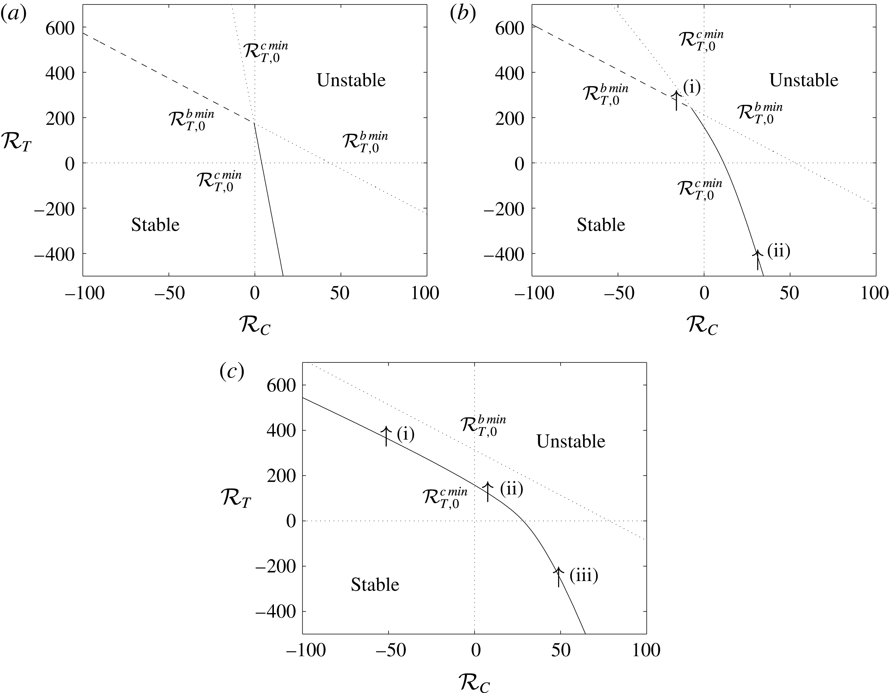
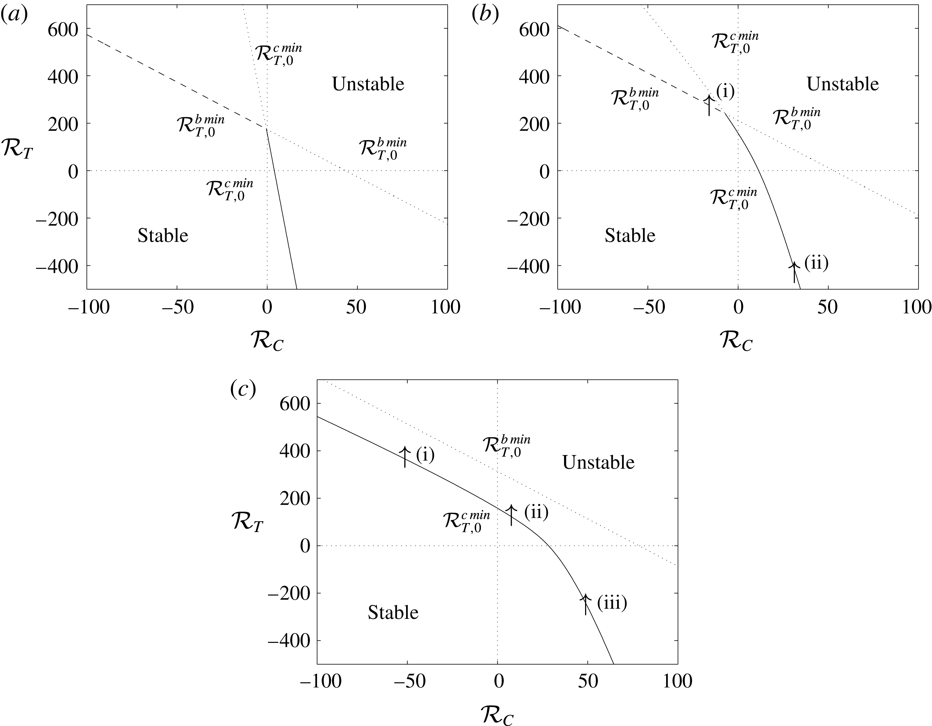
. Figure 2 illustrates the evolution of these stability boundaries in the
 $({\mathcal{R}}_{C},{\mathcal{R}}_{T})$
plane as
 $k_{0}$
is increased from
 $0$
.
Linear stability boundaries for
 $\unicode[STIX]{x1D706}=0.25$
,
 $Le=10$
and (a)
 $k_{0}=0$
, (b)
 $k_{0}=5$
, (c)
 $k_{0}=20$
. The solid lines represent stability boundaries on which
 $\unicode[STIX]{x1D70E}_{0+}=0$
, the dashed lines represent stability boundaries on which
 $\text{Re}(\unicode[STIX]{x1D70E}_{0+})=0$
but
 $\text{Im}(\unicode[STIX]{x1D70E}_{0+})\neq 0$
, and the dotted lines represent the continuation of
 ${\mathcal{R}}_{T,0}^{b\,min}$
and
 ${\mathcal{R}}_{T,0}^{c\,min}$
above the boundary. The numbered arrows in (b) and (c) represent the transects taken when examining the stability of the full problem. (Replotted from Pritchard & Richardson (Reference Pritchard and Richardson2007).)
When
 $k_{0}=0$
(figure 2
a), the stability boundary is given by
 ${\mathcal{R}}_{T,0}^{b\,min}$
in the solutally stable (SS) regime
 ${\mathcal{R}}_{C}<0$
and by
 ${\mathcal{R}}_{T,0}^{c\,min}$
in the solutally unstable (SU) regime
 ${\mathcal{R}}_{C}>0$
. In the SS regime,
 $\text{Im}(\unicode[STIX]{x1D70E}_{0+})\neq 0$
on the stability boundary, and so the onset of convection is by an oscillatory mode, whereas in the SU regime,
 $\text{Im}(\unicode[STIX]{x1D70E}_{0+})=0$
on the stability boundary, and the transition to instability is by a monotonically growing mode. Furthermore, in the SS regime,
 ${\mathcal{R}}_{T,0}^{b\,min}$
increases as
 ${\mathcal{R}}_{C}$
decreases: a greater destabilising temperature gradient is required to overcome a greater stabilising concentration gradient and allow the system to become unstable.
As the Damköhler number increases, the boundary
 ${\mathcal{R}}_{T,0}^{b\,min}$
moves up everywhere; meanwhile,
 ${\mathcal{R}}_{T,0}^{c\,min}$
moves upwards and rightwards in the SU regime (
 ${\mathcal{R}}_{C}>0$
) and downwards in the SS regime (
 ${\mathcal{R}}_{C}<0$
). The consequence is that when the Damköhler number is increased to
 $k_{0}=5$
(figure 2
b), the system becomes more stable in both regimes. However, when the Damköhler number is increased further to
 $k_{0}=20$
(figure 2
c), the system becomes more stable only in the SU regime. In the SS regime, the boundary
 ${\mathcal{R}}_{T,0}^{c\,min}$
has now passed entirely below the boundary
 ${\mathcal{R}}_{T,0}^{b\,min}$
, and so the transition to instability is by a monotonic rather than an oscillatory mode in both regimes. In particular, the stability boundary in the SS regime has now moved down from its original position, and the ‘reaction’ term now destabilises the system by weakening the stabilising solutal perturbations. Hence, a lower value of
 ${\mathcal{R}}_{T}$
is required for instability in the SS regime when
 $k_{0}=20$
than when
 $k_{0}=0$
.
The critical Damköhler number
 $k_{0}^{crit}$
at which the boundary
 ${\mathcal{R}}_{T,0}^{c\,min}$
passes entirely below the boundary
 ${\mathcal{R}}_{T,0}^{b\,min}$
is given by
 $$\begin{eqnarray}\displaystyle k_{0}^{crit}=\frac{\unicode[STIX]{x03C0}^{2}}{1-\unicode[STIX]{x1D706}}\left(1-\frac{1}{Le}\right). & & \displaystyle\end{eqnarray}$$
3.2 Linear stability analysis of the full problem
When
 $\unicode[STIX]{x1D6FF}\neq 0$
, an analytical solution of (3.17) in terms of
 $\unicode[STIX]{x1D70E}$
is not available. Therefore, we followed the approach of Ritchie & Pritchard (Reference Ritchie and Pritchard2011) for solutal convection and investigated the stability problem numerically using a continuation method, tracking
 $\unicode[STIX]{x1D70E}$
as
 ${\mathcal{R}}_{T}$
was changed while keeping
 ${\mathcal{R}}_{C}$
and all other parameters fixed. A numerical solution of (3.17) with
 $\unicode[STIX]{x1D6FF}=0$
and for a large value of
 ${\mathcal{R}}_{T}$
was used as an initial guess.
The task of tracking each solution branch is numerically very laborious, largely because the analytical solutions for
 $q_{i}$
are prohibitively complicated and so nested numerical solutions of (3.13) and (3.21) are required. As with the solutal convection problem (Ritchie & Pritchard Reference Ritchie and Pritchard2011), we found that to track a single branch it was necessary to reduce
 ${\mathcal{R}}_{T}$
in steps no larger than
 $10^{-2}$
, with smaller steps required around the bifurcation points discussed below. Additionally, to track the bifurcation point accurately, we needed to further simplify the determinant (3.17). Using column operations, the determinant can be simplified to
 $$\begin{eqnarray}\displaystyle (\text{e}^{q_{2}}-\text{e}^{q_{1}})(\text{e}^{q_{4}}-\text{e}^{q_{3}})(\text{e}^{q_{6}}-\text{e}^{q_{5}})(\text{e}^{q_{3}}-\text{e}^{q_{1}})(\text{e}^{q_{5}}-\text{e}^{q_{1}})\det (\unicode[STIX]{x1D63E})=0, & & \displaystyle\end{eqnarray}$$
where
 $\det (\unicode[STIX]{x1D63E})$
is omitted here for brevity (see Corson (Reference Corson2012, Appendix A.3)). When
 $\unicode[STIX]{x1D6FF}\neq 0$
,
 $$\begin{eqnarray}\displaystyle (\text{e}^{q_{2}}-\text{e}^{q_{1}})(\text{e}^{q_{4}}-\text{e}^{q_{3}})(\text{e}^{q_{6}}-\text{e}^{q_{5}})(\text{e}^{q_{3}}-\text{e}^{q_{1}})(\text{e}^{q_{5}}-\text{e}^{q_{1}})\neq 0. & & \displaystyle\end{eqnarray}$$
Therefore, to track each solution branch, we only require to solve
 $\det (\unicode[STIX]{x1D63E})=0$
. Nevertheless, each set of plots within figures 3 and 4 took around 12 h to produce on a desktop computer. This effectively precluded the thorough investigation of the full problem defined by (3.21); instead, we employed a less formal Galerkin approach in order to both search parameter space and provide insight into the solution structure.
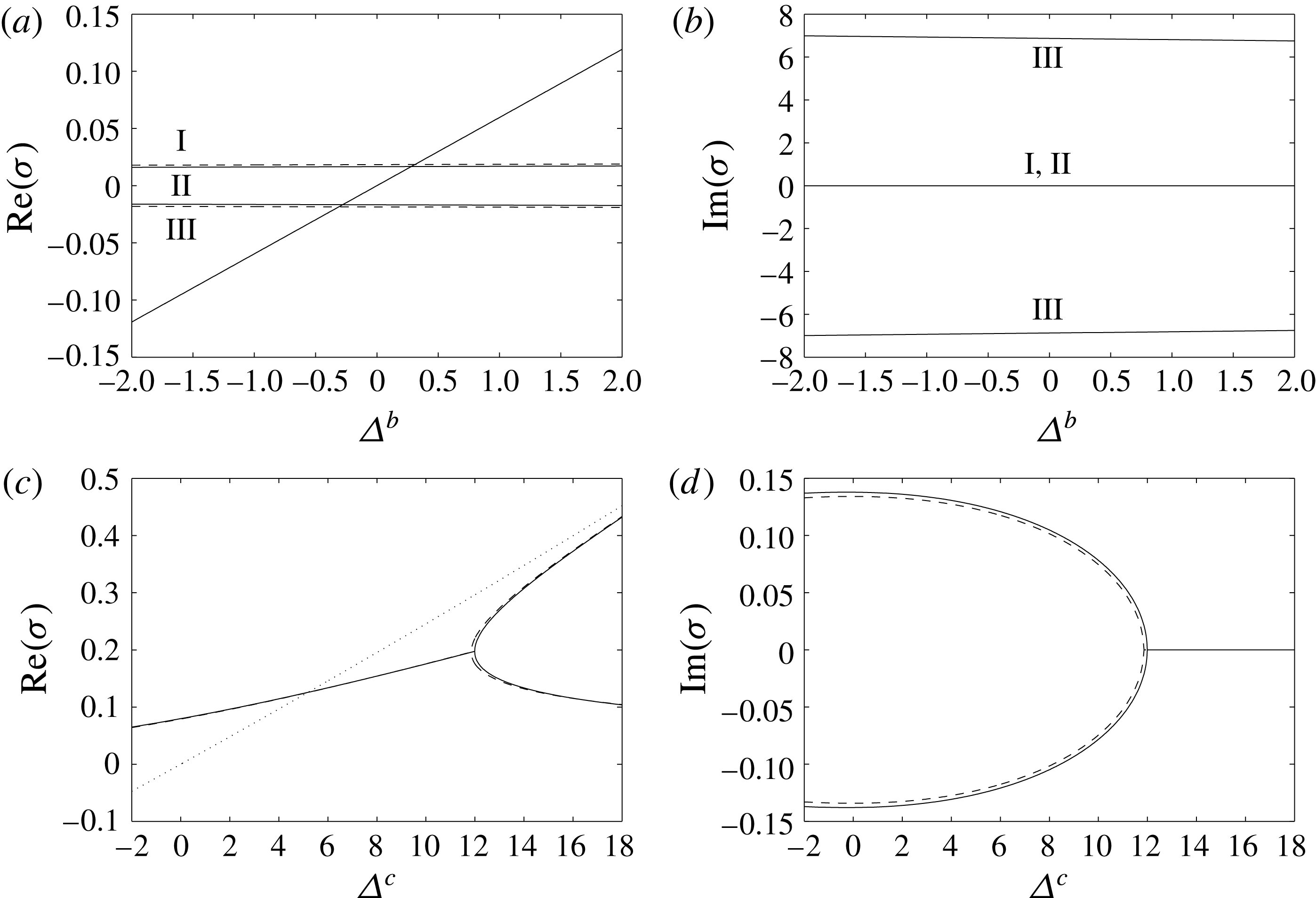
Behaviour of
 $\unicode[STIX]{x1D70E}$
for
 $k_{0}=5$
,
 $Le=10$
,
 $\unicode[STIX]{x1D706}=0.25$
,
 $\unicode[STIX]{x1D6FC}=3$
, and (a,b)
 ${\mathcal{R}}_{C}=-15$
,
 $\unicode[STIX]{x1D6FF}=-0.1$
close to
 $\unicode[STIX]{x1D6E5}^{b}=0$
, (c,d)
 ${\mathcal{R}}_{C}=30$
,
 $\unicode[STIX]{x1D6FF}=0.1$
close to
 $\unicode[STIX]{x1D6E5}^{c}=0$
. Panels (a,c) show
 $\text{Re}(\unicode[STIX]{x1D70E})$
, while (b,d) show
 $\text{Im}(\unicode[STIX]{x1D70E})$
. The solid lines are full numerical solutions to the linear problem, the dashed lines are Galerkin solutions and the dotted lines in (a,c) show the results for
 $\unicode[STIX]{x1D6FF}=0$
. The Roman numerals in (a,b) are to aid in identifying the corresponding real and imaginary parts of each
 $\unicode[STIX]{x1D70E}$
branch.

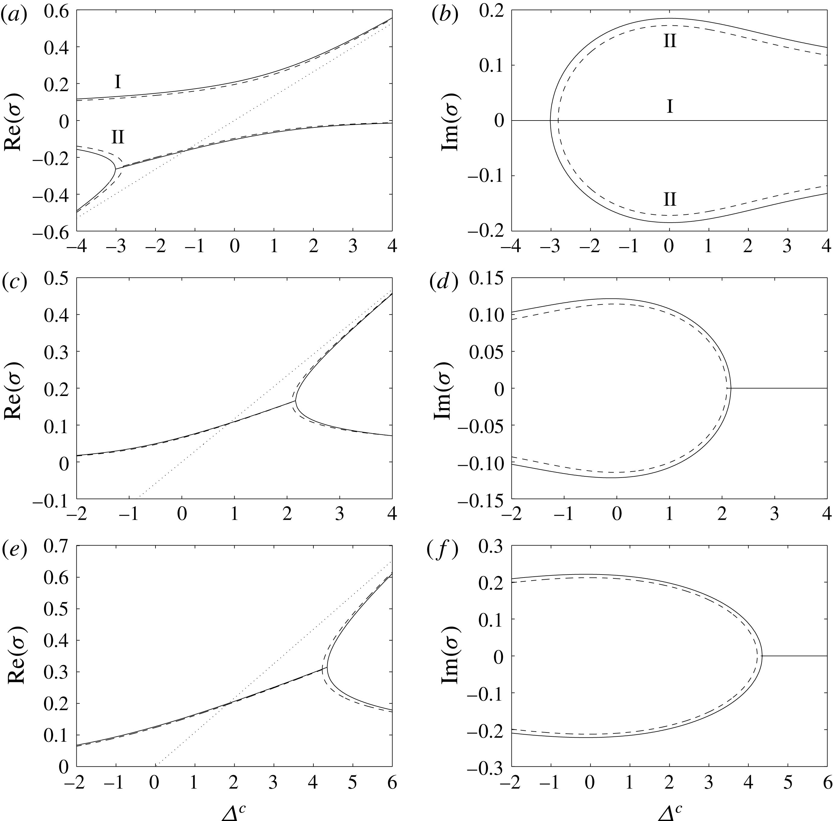
Behaviour of
 $\unicode[STIX]{x1D70E}$
close to
 $\unicode[STIX]{x1D6E5}^{c}=0$
, for
 $k_{0}=20$
,
 $Le=10$
,
 $\unicode[STIX]{x1D706}=0.25$
,
 $\unicode[STIX]{x1D6FC}=3$
, and (a,b)
 ${\mathcal{R}}_{C}=-50$
,
 $\unicode[STIX]{x1D6FF}=-0.1$
, (c,d)
 ${\mathcal{R}}_{C}=10$
,
 $\unicode[STIX]{x1D6FF}=0.1$
, (e,f)
 ${\mathcal{R}}_{C}=50$
,
 $\unicode[STIX]{x1D6FF}=0.1$
. Panels (a,c,e) show
 $\text{Re}(\unicode[STIX]{x1D70E})$
, while (b,d,f) show
 $\text{Im}(\unicode[STIX]{x1D70E})$
. The solid lines are full numerical solutions to the linear problem, the dashed lines are Galerkin solutions and the dotted lines in (a,c,e) show the results for
 $\unicode[STIX]{x1D6FF}=0$
. The Roman numerals in (a,b) are to aid in identifying the corresponding real and imaginary parts of each
 $\unicode[STIX]{x1D70E}$
branch.

3.3 Galerkin approach to the linear stability problem
We start with the system of equations (3.7)–(3.10), subject to the boundary conditions
 $$\begin{eqnarray}\displaystyle \unicode[STIX]{x1D6F9}=0,\quad \unicode[STIX]{x1D6E9}=0\quad \text{and}\quad \unicode[STIX]{x1D712}=0\quad \text{on}~z=0~\text{and}~z=1, & & \displaystyle\end{eqnarray}$$
and to the usual non-triviality condition that the solution is not identically zero. Rearranging (3.10), we see that
 $$\begin{eqnarray}\displaystyle \unicode[STIX]{x1D6F7}(z)=\frac{\unicode[STIX]{x1D6FF}k_{0}\unicode[STIX]{x1D719}_{0}(\unicode[STIX]{x1D6E9}(z)-\unicode[STIX]{x1D712}(z))}{\unicode[STIX]{x1D70E}}, & & \displaystyle\end{eqnarray}$$
and we can eliminate
 $\unicode[STIX]{x1D6F7}(z)$
from (3.9) to obtain the system
 $$\begin{eqnarray}\displaystyle & \displaystyle \left(\frac{\text{d}^{2}}{\text{d}z^{2}}-\unicode[STIX]{x1D6FC}^{2}\right)\unicode[STIX]{x1D6F9}(z)=-\text{i}\unicode[STIX]{x1D6FC}\left({\mathcal{R}}_{T}\unicode[STIX]{x1D6E9}(z)+{\mathcal{R}}_{C}\unicode[STIX]{x1D712}(z)\right), & \displaystyle\end{eqnarray}$$
 $$\begin{eqnarray}\displaystyle & \displaystyle \left(\frac{\text{d}^{2}}{\text{d}z^{2}}-\unicode[STIX]{x1D6FC}^{2}-\unicode[STIX]{x1D70E}\right)\unicode[STIX]{x1D6E9}(z)=\text{i}\unicode[STIX]{x1D6FC}\unicode[STIX]{x1D706}\unicode[STIX]{x1D6F9}(z), & \displaystyle\end{eqnarray}$$
 $$\begin{eqnarray}\displaystyle & \displaystyle \left(\frac{1}{Le}\left(\frac{\text{d}^{2}}{\text{d}z^{2}}-\unicode[STIX]{x1D6FC}^{2}\right)-k_{0}-\unicode[STIX]{x1D70E}\!\right)\unicode[STIX]{x1D712}(z)=\text{i}\unicode[STIX]{x1D6FC}\unicode[STIX]{x1D6F9}(z)-\frac{1}{Le}\frac{\unicode[STIX]{x1D6FF}k_{0}}{\unicode[STIX]{x1D70E}}\left(\frac{\text{d}}{\text{d}z}\unicode[STIX]{x1D6E9}(z)-\frac{\text{d}}{\text{d}z}\unicode[STIX]{x1D712}(z)\!\right)-k_{0}\unicode[STIX]{x1D6E9}(z), & \displaystyle \nonumber\\ \displaystyle & & \displaystyle\end{eqnarray}$$
subject to the same boundary conditions.
We seek approximate solutions of the form
 $$\begin{eqnarray}\displaystyle & \displaystyle \unicode[STIX]{x1D6F9}(z)=\sin (\unicode[STIX]{x03C0}z)+\unicode[STIX]{x1D6F9}_{2}\sin (2\unicode[STIX]{x03C0}z), & \displaystyle\end{eqnarray}$$
 $$\begin{eqnarray}\displaystyle & \displaystyle \unicode[STIX]{x1D6E9}(z)=\unicode[STIX]{x1D6E9}_{1}\sin (\unicode[STIX]{x03C0}z)+\unicode[STIX]{x1D6E9}_{2}\sin (2\unicode[STIX]{x03C0}z), & \displaystyle\end{eqnarray}$$
 $$\begin{eqnarray}\displaystyle & \displaystyle \unicode[STIX]{x1D712}(z)=\unicode[STIX]{x1D712}_{1}\sin (\unicode[STIX]{x03C0}z)+\unicode[STIX]{x1D712}_{2}\sin (2\unicode[STIX]{x03C0}z). & \displaystyle\end{eqnarray}$$
It should be noted that the boundary conditions are automatically satisfied and that the non-triviality condition has been imposed by normalising the
 $\sin (\unicode[STIX]{x03C0}z)$
component of
 $\unicode[STIX]{x1D6F9}(z)$
. In the limit
 $\unicode[STIX]{x1D6FF}=0$
, this approximation will become exact with
 $\unicode[STIX]{x1D6F9}_{2}=\unicode[STIX]{x1D6E9}_{2}=\unicode[STIX]{x1D712}_{2}=0$
.
With six unknowns, we can choose to satisfy six integral conditions. The natural ones are obtained by extracting the first and second Fourier sine components of (3.25)–(3.27),
 $$\begin{eqnarray}\displaystyle & \displaystyle \int _{0}^{1}\sin (\unicode[STIX]{x03C0}nz)\left[\frac{\text{d}^{2}\unicode[STIX]{x1D6F9}}{\text{d}z^{2}}-\unicode[STIX]{x1D6FC}^{2}\unicode[STIX]{x1D6F9}\right]\text{d}z=\int _{0}^{1}\sin (\unicode[STIX]{x03C0}nz)\left[-\text{i}\unicode[STIX]{x1D6FC}{\mathcal{R}}_{T}\unicode[STIX]{x1D6E9}-\text{i}\unicode[STIX]{x1D6FC}{\mathcal{R}}_{C}\unicode[STIX]{x1D712}\right]\text{d}z, & \displaystyle\end{eqnarray}$$
 $$\begin{eqnarray}\displaystyle & \displaystyle \int _{0}^{1}\sin (\unicode[STIX]{x03C0}nz)\left[\frac{\text{d}^{2}\unicode[STIX]{x1D6E9}}{\text{d}z^{2}}-\unicode[STIX]{x1D6FC}^{2}\unicode[STIX]{x1D6E9}-\unicode[STIX]{x1D70E}\unicode[STIX]{x1D6E9}\right]\text{d}z=\int _{0}^{1}\sin (\unicode[STIX]{x03C0}nz)[\text{i}\unicode[STIX]{x1D6FC}\unicode[STIX]{x1D706}\unicode[STIX]{x1D6F9}]\,\text{d}z, & \displaystyle\end{eqnarray}$$
 $$\begin{eqnarray}\displaystyle & & \displaystyle \int _{0}^{1}\sin (\unicode[STIX]{x03C0}nz)\left[\frac{1}{Le}\left(\frac{\text{d}^{2}\unicode[STIX]{x1D712}}{\text{d}z^{2}}-\unicode[STIX]{x1D6FC}^{2}\unicode[STIX]{x1D712}\right)-(k_{0}+\unicode[STIX]{x1D70E})\unicode[STIX]{x1D712}\right]\text{d}z\nonumber\\ \displaystyle & & \displaystyle \quad =\int _{0}^{1}\sin (\unicode[STIX]{x03C0}nz)\left[\text{i}\unicode[STIX]{x1D6FC}\unicode[STIX]{x1D6F9}-\frac{1}{Le}\frac{\unicode[STIX]{x1D6FF}k_{0}}{\unicode[STIX]{x1D70E}}\left(\frac{\text{d}\unicode[STIX]{x1D6E9}}{\text{d}z}-\frac{\text{d}\unicode[STIX]{x1D712}}{\text{d}z}\right)-k_{0}\unicode[STIX]{x1D6E9}\right]\text{d}z,\end{eqnarray}$$
for
 $n=1$
and for
 $n=2$
. This yields a system of six algebraic equations,
 $$\begin{eqnarray}\displaystyle & \displaystyle -\frac{1}{2}(\unicode[STIX]{x03C0}^{2}+\unicode[STIX]{x1D6FC}^{2})=-\frac{\text{i}\unicode[STIX]{x1D6FC}}{2}\left({\mathcal{R}}_{T}\unicode[STIX]{x1D6E9}_{1}+{\mathcal{R}}_{C}\unicode[STIX]{x1D712}_{1}\right), & \displaystyle\end{eqnarray}$$
 $$\begin{eqnarray}\displaystyle & \displaystyle -\frac{1}{2}(4\unicode[STIX]{x03C0}^{2}+\unicode[STIX]{x1D6FC}^{2})\unicode[STIX]{x1D6F9}_{2}=-\frac{\text{i}\unicode[STIX]{x1D6FC}}{2}\left({\mathcal{R}}_{T}\unicode[STIX]{x1D6E9}_{2}+{\mathcal{R}}_{C}\unicode[STIX]{x1D712}_{2}\right), & \displaystyle\end{eqnarray}$$
 $$\begin{eqnarray}\displaystyle & \displaystyle -{\textstyle \frac{1}{2}}(\unicode[STIX]{x03C0}^{2}+\unicode[STIX]{x1D6FC}^{2}+\unicode[STIX]{x1D70E})\unicode[STIX]{x1D6E9}_{1}={\textstyle \frac{1}{2}}\text{i}\unicode[STIX]{x1D6FC}\unicode[STIX]{x1D706}, & \displaystyle\end{eqnarray}$$
 $$\begin{eqnarray}\displaystyle & \displaystyle -{\textstyle \frac{1}{2}}(4\unicode[STIX]{x03C0}^{2}+\unicode[STIX]{x1D6FC}^{2}+\unicode[STIX]{x1D70E})\unicode[STIX]{x1D6E9}_{2}={\textstyle \frac{1}{2}}\text{i}\unicode[STIX]{x1D6FC}\unicode[STIX]{x1D706}\unicode[STIX]{x1D6F9}_{2}, & \displaystyle\end{eqnarray}$$
 $$\begin{eqnarray}\displaystyle & \displaystyle -\frac{1}{2}\frac{1}{Le}(\unicode[STIX]{x03C0}^{2}+\unicode[STIX]{x1D6FC}^{2}+Le(k_{0}+\unicode[STIX]{x1D70E}))\unicode[STIX]{x1D712}_{1}=\frac{1}{2}(\text{i}\unicode[STIX]{x1D6FC}-k_{0}\unicode[STIX]{x1D6E9}_{1})+\frac{4}{3}\frac{1}{Le}\frac{\unicode[STIX]{x1D6FF}k_{0}}{\unicode[STIX]{x1D70E}}(\unicode[STIX]{x1D6E9}_{2}-\unicode[STIX]{x1D712}_{2}), & \displaystyle\end{eqnarray}$$
 $$\begin{eqnarray}\displaystyle & \displaystyle -\frac{1}{2}\frac{1}{Le}(4\unicode[STIX]{x03C0}^{2}+\unicode[STIX]{x1D6FC}^{2}+Le(k_{0}+\unicode[STIX]{x1D70E}))\unicode[STIX]{x1D712}_{2}=\frac{1}{2}(\text{i}\unicode[STIX]{x1D6FC}\unicode[STIX]{x1D6F9}_{2}-k_{0}\unicode[STIX]{x1D6E9}_{2})+\frac{4}{3}\frac{1}{Le}\frac{\unicode[STIX]{x1D6FF}k_{0}}{\unicode[STIX]{x1D70E}}(\unicode[STIX]{x1D712}_{1}-\unicode[STIX]{x1D6E9}_{1}). & \displaystyle\end{eqnarray}$$
We can then eliminate
 $\unicode[STIX]{x1D6F9}_{2}$
,
 $\unicode[STIX]{x1D6E9}_{1}$
,
 $\unicode[STIX]{x1D6E9}_{2}$
,
 $\unicode[STIX]{x1D712}_{1}$
and
 $\unicode[STIX]{x1D712}_{2}$
, and find that
 $\unicode[STIX]{x1D70E}$
satisfies the sextic
 $$\begin{eqnarray}\displaystyle a_{6}\unicode[STIX]{x1D70E}^{6}+a_{5}\unicode[STIX]{x1D70E}^{5}+a_{4}\unicode[STIX]{x1D70E}^{4}+a_{3}\unicode[STIX]{x1D70E}^{3}+a_{2}\unicode[STIX]{x1D70E}^{2}+a_{1}\unicode[STIX]{x1D70E}+a_{0}=0, & & \displaystyle\end{eqnarray}$$
where the coefficients
 $a_{i}$
are omitted here for brevity. It is straightforward to locate all of the complex roots of (3.40) numerically, for example using the fsolve command in Maple, and thus to track all of the solutions through parameter space.
3.3.1 Behaviour of the roots
 $\unicode[STIX]{x1D70E}$

To examine the behaviour of
 $\unicode[STIX]{x1D70E}$
, it is helpful to express the thermal Rayleigh number in terms of the critical conditions for
 $\unicode[STIX]{x1D6FF}=0$
. We define
 ${\mathcal{R}}_{T}={\mathcal{R}}_{T,0}^{b}({\mathcal{R}}_{C},\unicode[STIX]{x1D6FC})+\unicode[STIX]{x1D6E5}^{b}$
and
 ${\mathcal{R}}_{T}={\mathcal{R}}_{T,0}^{c}({\mathcal{R}}_{C},\unicode[STIX]{x1D6FC})+\unicode[STIX]{x1D6E5}^{c}$
. In this and future sections, we will focus on two values of the Damköhler number: a subcritical value
 $k_{0}=5$
and a supercritical value
 $k_{0}=20$
. When
 $k_{0}=5$
, the stability boundary is given by
 ${\mathcal{R}}_{T,0}^{b}$
for
 ${\mathcal{R}}_{C}\lesssim -10$
and by
 ${\mathcal{R}}_{T,0}^{c}$
for
 ${\mathcal{R}}_{C}\gtrsim -10$
(figure 2
b). When
 $k_{0}=20$
, the stability boundary is given solely by
 ${\mathcal{R}}_{T,0}^{c}$
(figure 2
c).
Figures 3 and 4 show the behaviour of
 $\unicode[STIX]{x1D70E}$
as
 ${\mathcal{R}}_{C}$
is increased for
 $k_{0}=5$
and
 $k_{0}=20$
respectively, where the wavenumber
 $\unicode[STIX]{x1D6FC}$
and all other parameters except
 $\unicode[STIX]{x1D6E5}^{c}$
are fixed. For these figures, and all subsequent figures in this section, the default parameters were
 $\unicode[STIX]{x1D719}_{0}=0.1$
,
 $Le=10$
,
 $\unicode[STIX]{x1D706}=0.25$
, and
 $\unicode[STIX]{x1D6FF}=0.1$
for
 ${\mathcal{R}}_{C}>0$
,
 $\unicode[STIX]{x1D6FF}=-0.1$
for
 ${\mathcal{R}}_{C}<0$
. The large value of
 $|\unicode[STIX]{x1D6FF}|$
and the moderate value of
 $Le$
were chosen to make deviations from the
 $\unicode[STIX]{x1D6FF}=0$
case as apparent as possible. (We note that in practice the value of
 $Le$
may be large, and since
 $\unicode[STIX]{x1D6FF}$
appears in the linearised equations (3.1)–(3.4) only in the combination
 $\unicode[STIX]{x1D6FF}/Le$
, this reduces the rate at which the matrix evolves. It can be shown that the stability problem is otherwise regular in the asymptotic limit of large
 $Le$
; we do not pursue this limit further here.)
For
 $k_{0}=5$
, we consider two different values of
 ${\mathcal{R}}_{C}$
(indicated by the numbered arrows in figure 2
b) in order to cross both stability boundaries: (i)
 ${\mathcal{R}}_{C}=-15$
, so that
 ${\mathcal{R}}_{T,0}^{c}>0$
and we have a stabilising solutal gradient and a destabilising temperature gradient; (ii)
 ${\mathcal{R}}_{C}=30$
, so that
 ${\mathcal{R}}_{T,0}^{c}<0$
and we have a destabilising solutal gradient and a stabilising temperature gradient.
We first consider
 ${\mathcal{R}}_{C}=-15$
(figure 3
a,b). When
 $\unicode[STIX]{x1D6FF}=0$
, the stability boundary is given by
 ${\mathcal{R}}_{T}={\mathcal{R}}_{T,0}^{b}$
(figure 2
b) and the transition to instability is through a growing oscillatory mode where
 $\text{Im}(\unicode[STIX]{x1D70E})\neq 0$
. When
 $\unicode[STIX]{x1D6E5}^{b}$
is large and positive, the dominant
 $\unicode[STIX]{x1D70E}$
branch (III) very closely follows that of
 $\unicode[STIX]{x1D70E}_{0+}$
. However, below
 $\unicode[STIX]{x1D6E5}^{b}\approx 0.3$
, the dominant branch switches to one (I) that appears to asymptote to zero as
 $\unicode[STIX]{x1D6E5}^{b}\rightarrow -\infty$
, with
 $\text{Im}(\unicode[STIX]{x1D70E})=0$
.
When
 ${\mathcal{R}}_{C}=30$
(figure 3
c,d), the branch of
 $\unicode[STIX]{x1D70E}$
with the largest real part closely tracks the
 $\unicode[STIX]{x1D70E}_{0+}$
branch when
 $\unicode[STIX]{x1D6E5}^{c}$
is large and positive. It deviates weakly from this as
 $\unicode[STIX]{x1D6E5}^{c}$
is reduced, until this branch and the one below merge. This occurs at
 $\unicode[STIX]{x1D6E5}^{c}\approx 11.8$
, and at this bifurcation point the values of
 $\unicode[STIX]{x1D70E}$
become complex. As
 $\unicode[STIX]{x1D6E5}^{c}$
is further reduced,
 $\text{Re}(\unicode[STIX]{x1D70E})$
continues to fall and asymptotes to zero as
 $\unicode[STIX]{x1D6E5}^{c}\rightarrow -\infty$
. The behaviour of the stability branches is very similar to that seen in solutal convection (Ritchie & Pritchard Reference Ritchie and Pritchard2011, figure 2).
For
 $k_{0}=20$
, we consider three different values of
 ${\mathcal{R}}_{C}$
, as indicated by the numbered arrows in figure 2(c), in order to cover the three regimes of interest in double diffusive convection: (i)
 ${\mathcal{R}}_{C}=-50$
, so that
 ${\mathcal{R}}_{T,0}^{c}>0$
and we have a stabilising solutal gradient and a destabilising temperature gradient; (ii)
 ${\mathcal{R}}_{C}=10$
, so that
 ${\mathcal{R}}_{T,0}^{c}>0$
and we have destabilising solutal and temperature gradients; (iii)
 ${\mathcal{R}}_{C}=50$
, so that
 ${\mathcal{R}}_{T,0}^{c}<0$
and we have a destabilising solutal gradient and a stabilising temperature gradient.
We first consider
 ${\mathcal{R}}_{C}=-50$
(figure 4
a,b). When
 $\unicode[STIX]{x1D6E5}^{c}$
is large and positive, the branch of
 $\unicode[STIX]{x1D70E}$
with the largest real part (I) closely tracks the
 $\unicode[STIX]{x1D70E}_{0+}$
branch. As
 $\unicode[STIX]{x1D6E5}^{c}$
is reduced,
 $\unicode[STIX]{x1D70E}$
deviates from the
 $\unicode[STIX]{x1D70E}_{0+}$
branch and asymptotes to zero from above as
 $\unicode[STIX]{x1D6E5}^{c}\rightarrow -\infty$
. Along this branch,
 $\text{Im}(\unicode[STIX]{x1D70E})=0$
. The subdominant
 $\unicode[STIX]{x1D70E}$
branch (II) also displays some interesting behaviour. As
 $\unicode[STIX]{x1D6E5}^{c}\rightarrow \infty$
,
 $\text{Re}(\unicode[STIX]{x1D70E})$
tends to zero from below, with
 $\text{Im}(\unicode[STIX]{x1D70E})\neq 0$
. As
 $\unicode[STIX]{x1D6E5}^{c}$
is reduced,
 $\text{Re}(\unicode[STIX]{x1D70E})$
decreases until
 $\unicode[STIX]{x1D6E5}^{c}\approx -2.9$
, where this branch bifurcates, with the upper branch tending to zero from below and the lower branch tending to
 $\unicode[STIX]{x1D70E}_{0+}$
as
 $\unicode[STIX]{x1D6E5}^{c}\rightarrow -\infty$
. At the bifurcation point, the values of
 $\unicode[STIX]{x1D70E}$
become strictly real.
We next consider
 ${\mathcal{R}}_{C}=10$
(figure 4
c,d) and
 ${\mathcal{R}}_{C}=50$
(figure 4
e,f). In each case, we have a destabilising solutal gradient and the behaviour of the
 $\unicode[STIX]{x1D70E}$
branches is very similar to that seen with
 $k_{0}=5$
(figure 3
e,f), as well as to that seen in solutal convection (Ritchie & Pritchard Reference Ritchie and Pritchard2011, figure 2). In each case, the position of the bifurcation point changes. When
 ${\mathcal{R}}_{C}=10$
(figure 4
c,d), the bifurcation occurs at
 $\unicode[STIX]{x1D6E5}^{c}\approx 2.2$
, and when
 ${\mathcal{R}}_{C}=50$
(figure 4
e,f), it occurs at
 $\unicode[STIX]{x1D6E5}^{c}\approx 4.3$
. It can be shown that the bifurcation point scales as
 $\unicode[STIX]{x1D6E5}^{c}\sim |\unicode[STIX]{x1D6FF}|^{2/3}$
and
 $\unicode[STIX]{x1D70E}\sim |\unicode[STIX]{x1D6FF}|^{2/3}$
(Corson Reference Corson2012, § 5.4.2).
Figures 3 and 4 also compare the predictions of the Galerkin analysis with those from the full numerical solution of (3.21). In each case, good agreement can be seen, with errors in the imaginary part of the order of 10 % or smaller. It should be noted that full solutions for the subdominant branches were obtained by using the Galerkin solution as an initial guess.
It is clear that there are three different scenarios of interest, which depend on the signs of the underlying thermal and solutal gradients. The first scenario occurs when the solutal gradient is destabilising and, regardless of the thermal gradient, the behaviour of
 $\unicode[STIX]{x1D70E}$
closely resembles that seen in Ritchie & Pritchard (Reference Ritchie and Pritchard2011) for solutal convection. This similarity in behaviour is unsurprising since faster thermal diffusion means that the thermal gradient is of secondary importance in solute-driven convection. In the second and third scenarios, the solutal gradient is stabilising and the thermal gradient is destabilising. If the Damköhler number is subcritical, then the dominant branch switches from being strictly real to complex as
 $\unicode[STIX]{x1D6E5}^{b}$
increases (figure 3
a,b), whereas if the Damköhler number is supercritical, then the dominant branch remains strictly real as
 $\unicode[STIX]{x1D6E5}^{c}$
increases (figure 4
a,b).
3.4 Eigenfunction structure and instability mechanism
As well as providing the complex growth rate
 $\unicode[STIX]{x1D70E}$
, the Galerkin stability analysis also provides the quantities
 $W_{2}$
,
 $\unicode[STIX]{x1D6E9}_{1}$
,
 $\unicode[STIX]{x1D6E9}_{2}$
,
 $\unicode[STIX]{x1D712}_{1}$
and
 $\unicode[STIX]{x1D712}_{2}$
which define the corresponding vertical eigenfunction. To elucidate the mechanism involved in the instability, it is useful to examine these quantities.
We will consider three different scenarios, as described in the previous section: first, the combination of a destabilising solutal gradient with either a stabilising or a destabilising thermal gradient; second, a destabilising thermal gradient with a stabilising solutal gradient and a subcritical Damköhler number, so that the onset of instability is oscillatory; third, a destabilising thermal gradient with a stabilising solutal gradient and a supercritical Damköhler number.
In our formulation, when the thermal gradient is destabilising,
 $\hat{T}_{1}-\hat{T}_{0}<0$
, so
 $T^{\prime }<0$
in regions that become warmer than the base state and
 $T^{\prime }>0$
in regions that become cooler. Similarly, when the solutal gradient is stabilising,
 ${\hat{C}}_{1}-{\hat{C}}_{0}<0$
, so
 $C^{\prime }<0$
in regions of higher concentration and
 $C^{\prime }>0$
in regions of lower concentration. Therefore, in order to avoid confusion when considering the spatial structure of the fastest-growing eigenfunction, we define
 $\tilde{T}=-\text{sgn}({\mathcal{R}}_{T})T^{\prime }$
and
 $\tilde{C}=\text{sgn}({\mathcal{R}}_{C})C^{\prime }$
. With this reformulation,
 $\tilde{T}>0$
and
 $\tilde{C}>0$
will always correspond to regions of higher temperatures and concentrations respectively, while
 $\tilde{T}<0$
and
 $\tilde{C}<0$
will correspond to regions of lower temperatures and concentrations respectively. Using (3.24) and the definitions of
 $\tilde{T}$
and
 $\tilde{C}$
, we also define
 $$\begin{eqnarray}\displaystyle \tilde{\unicode[STIX]{x1D719}}=-\frac{\unicode[STIX]{x1D6FF}k_{0}\unicode[STIX]{x1D719}_{0}}{\unicode[STIX]{x1D70E}}(\text{sgn}({\mathcal{R}}_{T})\tilde{T}+\text{sgn}({\mathcal{R}}_{C})\tilde{C}), & & \displaystyle\end{eqnarray}$$
so that
 $\tilde{\unicode[STIX]{x1D719}}>0$
always corresponds to regions in which the porosity is greater than
 $\unicode[STIX]{x1D719}_{0}$
, while
 $\tilde{\unicode[STIX]{x1D719}}<0$
always corresponds to regions in which the porosity is lower than
 $\unicode[STIX]{x1D719}_{0}$
.
3.4.1 Scenario one: destabilising solutal gradient
We first consider the combination of a destabilising solutal gradient with either a stabilising or a destabilising thermal gradient. From (3.4), the porosity evolution is driven by the sum
 $\text{sgn}({\mathcal{R}}_{T})\tilde{T}+\text{sgn}({\mathcal{R}}_{C})\tilde{C}$
. Regardless of the direction of the thermal gradient, the amplitude of the concentration perturbation
 $\tilde{C}$
will always dominate the amplitude of the thermal perturbation
 $\tilde{T}$
since the diffusion of heat is much faster than the diffusion of solute through the fluid. Hence, these situations are analogous to those found in Ritchie & Pritchard (Reference Ritchie and Pritchard2011) for solutal convection in which the porosity evolution is driven solely by the concentration perturbation. Therefore, we will not discuss this scenario further here; the reader is referred to Corson (Reference Corson2012, § 5.4.3.1) for more details.
3.4.2 Scenario two: stabilising solutal gradient, destabilising thermal gradient, subcritical Damköhler number
In this and the subsequent section, we consider the combination of a stabilising solutal gradient with a destabilising thermal gradient. Here, we consider this combination along with a subcritical Damköhler number, so the transition to instability is through a growing oscillatory mode.
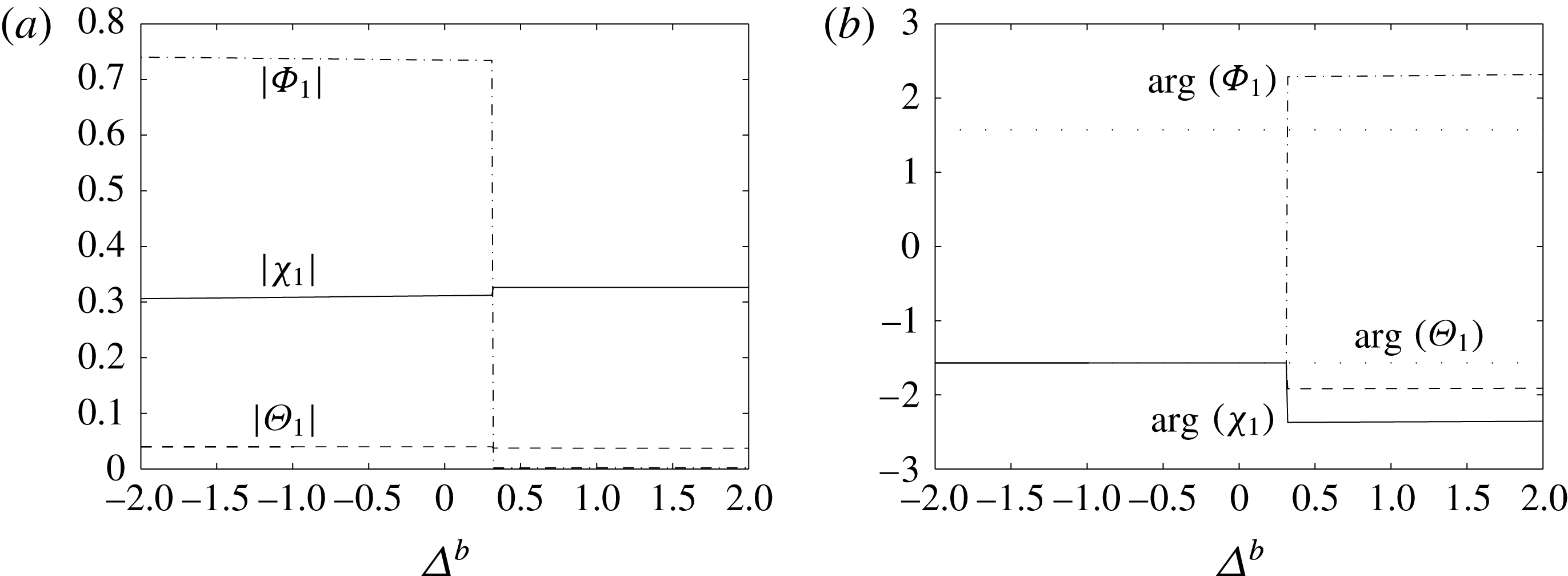
(a) Amplitudes and (b) relative phases of the first harmonics as functions of
 $\unicode[STIX]{x1D6E5}^{b}$
. In (a), the solid line is
 $|\unicode[STIX]{x1D712}_{1}|$
, the dashed line is
 $|\unicode[STIX]{x1D6E9}_{1}|$
and the dashed–dotted line is
 $|\unicode[STIX]{x1D6F7}_{1}|$
. In (b), the solid line is
 $\arg (\unicode[STIX]{x1D712}_{1})$
, the dashed line is
 $\arg (\unicode[STIX]{x1D6E9}_{1})$
and the dashed–dotted line is
 $\arg (\unicode[STIX]{x1D6F7}_{1})$
. The light dotted lines are
 $-\unicode[STIX]{x03C0}/2$
and
 $\unicode[STIX]{x03C0}/2$
. The parameter values are
 $\unicode[STIX]{x1D719}_{0}=0.1$
,
 $k_{0}=5$
,
 $\unicode[STIX]{x1D6FF}=-0.1$
,
 $\unicode[STIX]{x1D6FC}=3$
,
 $Le=10$
,
 $\unicode[STIX]{x1D706}=0.25$
,
 ${\mathcal{R}}_{C}=-15$
. The jump at
 $\unicode[STIX]{x1D6E5}^{b}\approx 0.4$
is a result of the change of dominant branch.

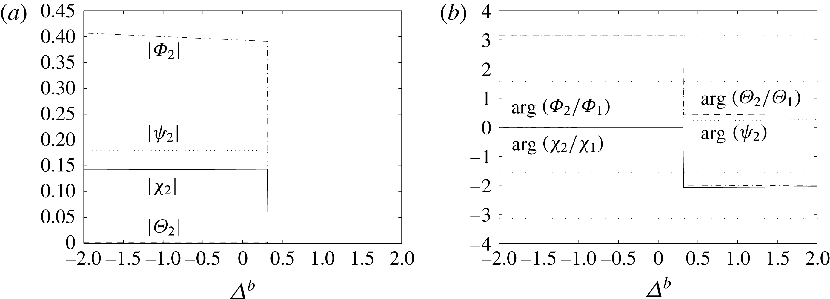
(a) Amplitudes and (b) relative phases of the second harmonics as functions of
 $\unicode[STIX]{x1D6E5}^{b}$
. In (a), the solid line is
 $|\unicode[STIX]{x1D712}_{2}|$
, the dashed line is
 $|\unicode[STIX]{x1D6E9}_{2}|$
, the dashed–dotted line is
 $|\unicode[STIX]{x1D6F7}_{2}|$
and the dotted line is
 $|\unicode[STIX]{x1D713}_{2}|$
. In (b), the solid line is
 $\arg (\unicode[STIX]{x1D712}_{2}/\unicode[STIX]{x1D712}_{1})$
, the dashed line is
 $\arg (\unicode[STIX]{x1D6E9}_{2}/\unicode[STIX]{x1D6E9}_{1})$
, the dashed–dotted line is
 $\arg (\unicode[STIX]{x1D6F7}_{2}/\unicode[STIX]{x1D6F7}_{1})$
and the dotted line is
 $\arg (\unicode[STIX]{x1D713}_{2})$
. The light dotted lines are
 $\unicode[STIX]{x03C0}$
,
 $\unicode[STIX]{x03C0}/2$
,
 $-\unicode[STIX]{x03C0}/2$
and
 $-\unicode[STIX]{x03C0}$
. The parameter values are
 $\unicode[STIX]{x1D719}_{0}=0.1$
,
 $k_{0}=5$
,
 $\unicode[STIX]{x1D6FF}=-0.1$
,
 $\unicode[STIX]{x1D6FC}=3$
,
 $Le=10$
,
 $\unicode[STIX]{x1D706}=0.25$
,
 ${\mathcal{R}}_{C}=-15$
. The jump at
 $\unicode[STIX]{x1D6E5}^{b}\approx 0.4$
is a result of the change of dominant branch.

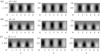
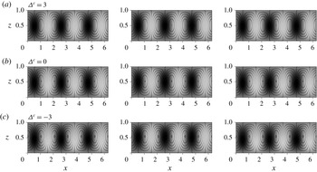
Eigenfunctions from the Galerkin analysis. Left-hand column: streamlines superimposed on the concentration perturbation
 $\tilde{C}$
. Centre column: streamlines superimposed on the temperature perturbation
 $\tilde{T}$
. Right-hand column: streamlines superimposed on the porosity perturbation
 $\tilde{\unicode[STIX]{x1D719}}$
. The parameter values are
 $\unicode[STIX]{x1D719}_{0}=0.1$
,
 $k_{0}=5$
,
 $\unicode[STIX]{x1D6FF}=-0.1$
,
 $\unicode[STIX]{x1D6FC}=3$
,
 $Le=10$
,
 $\unicode[STIX]{x1D706}=0.25$
,
 ${\mathcal{R}}_{C}=-15$
. In each case, the values of
 $\unicode[STIX]{x1D713}$
on the streamlines are evenly spaced, and in each plot, darker shading corresponds to lower values; scales are arbitrary.

Figures 5 and 6 show how the amplitudes and phases of the perturbations to the streamfunction, temperature, concentration and porosity vary as
 $\unicode[STIX]{x1D6E5}^{b}$
changes for
 $k_{0}=5$
and
 ${\mathcal{R}}_{C}=-15$
. They should be read in conjunction with figure 3(a,b), which illustrates the behaviour of
 $\unicode[STIX]{x1D70E}$
with
 $\unicode[STIX]{x1D6E5}^{c}$
, and figure 7, which illustrates how the corresponding spatial structure of the fastest-growing eigenfunction behaves as
 $\unicode[STIX]{x1D6E5}^{b}$
is reduced. We recall that at
 $\unicode[STIX]{x1D6E5}^{b}\approx 0.4$
we abruptly switch stability branches in order to remain on the dominant branch (figure 3
a,b). For values of
 $\unicode[STIX]{x1D6E5}^{b}\gtrsim 0.4$
, the dominant values of
 $\unicode[STIX]{x1D70E}$
are complex, but for
 $\unicode[STIX]{x1D6E5}^{b}\lesssim 0.4$
, the dominant values are strictly real.
For
 $\unicode[STIX]{x1D6E5}^{b}>0.4$
, the perturbations to concentration, temperature and porosity are all small (figure 5
a) and are approximately in phase (figure 5
b), such that the maxima of the first harmonics of
 $\tilde{C}$
and
 $\tilde{T}$
roughly coincide with the minima of the first harmonic of
 $\tilde{\unicode[STIX]{x1D719}}$
. The slight offset between extrema of
 $\tilde{C}$
,
 $\tilde{T}$
and
 $\tilde{\unicode[STIX]{x1D719}}$
can be seen more clearly in figure 7(a), but the pattern of flow, concentration, temperature and porosity is still very similar to that of simple convection: downflow draws down lower concentrations and temperatures from the upper boundary, while upflow draws up higher concentrations and temperatures. Upflow occurs in low-permeability regions and downflow in high-permeability regions.
A change is immediately noticeable when the dominant branch abruptly switches at
 $\unicode[STIX]{x1D6E5}^{b}\approx 0.4$
: the first harmonic of
 $\tilde{\unicode[STIX]{x1D719}}$
increases (figure 5
a), and the perturbations are now out of phase (figure 5
b), with the extrema of
 $\tilde{C}$
and
 $\tilde{T}$
moving leftwards, and the extrema of
 $\tilde{\unicode[STIX]{x1D719}}$
moving rightward relative to those of
 $\unicode[STIX]{x1D713}$
. The second harmonics are now all non-zero (figure 6
a), with the relative phases of the second harmonics of
 $\unicode[STIX]{x1D713}$
and
 $\tilde{T}$
equal to
 $\unicode[STIX]{x03C0}$
, and those of
 $\tilde{C}$
and
 $\tilde{\unicode[STIX]{x1D719}}$
equal to
 $0$
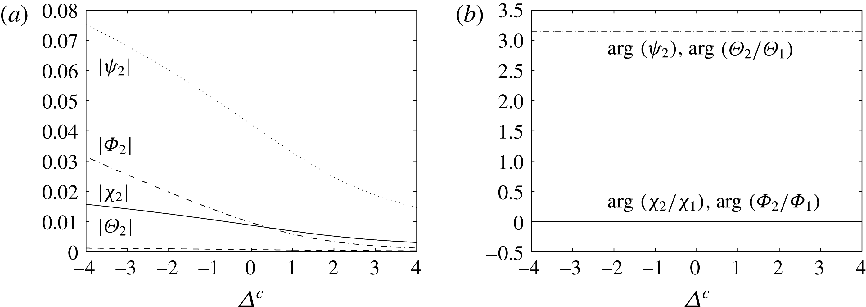
(figure 6
b). Therefore, the temperature and streamfunction fields are flattened upwards, whereas the concentration and porosity fields are flattened downwards. This can be seen in figure 7(b) for
 $\unicode[STIX]{x1D6E5}^{b}=0$
: downflow is now occurring in low-permeability regions and upflow in high-permeability regions, and it is evident that the circulation and temperature cells have moved upwards, but the porosity and concentration cells have moved downwards.
By comparing the magnitudes of the individual terms in (3.2) and (3.3) as
 $\unicode[STIX]{x1D6E5}^{b}$
is reduced, we can elucidate the mechanisms that cause the upward flattening of the circulation and temperature cells, and the downward flattening of the porosity and concentration cells. For
 $\unicode[STIX]{x1D6E5}^{b}>0.4$
, before the branch switch, the porosity perturbation is weak and the system is dominated by convection. After the branch switch, although vertical convection still balances with diffusion in the temperature perturbation equation (3.2), it now balances with the
 $\unicode[STIX]{x2202}\unicode[STIX]{x1D719}^{\prime }/\unicode[STIX]{x2202}z$
term in the concentration perturbation equation (3.3). This results in an offset between the porosity and circulation cells as faster vertical velocities must correspond to higher vertical porosity gradients. Therefore, the porosity cells move downwards and the circulation cells move upwards. This offset then results in the temperature cells moving upwards and the concentration cells moving downwards.
3.4.3 Scenario three: stabilising solutal gradient, destabilising thermal gradient, supercritical Damköhler number
We now consider the combination of a stabilising solutal gradient with a destabilising thermal gradient along with a supercritical Damköhler number, so the onset of convection is through a monotonic instability.
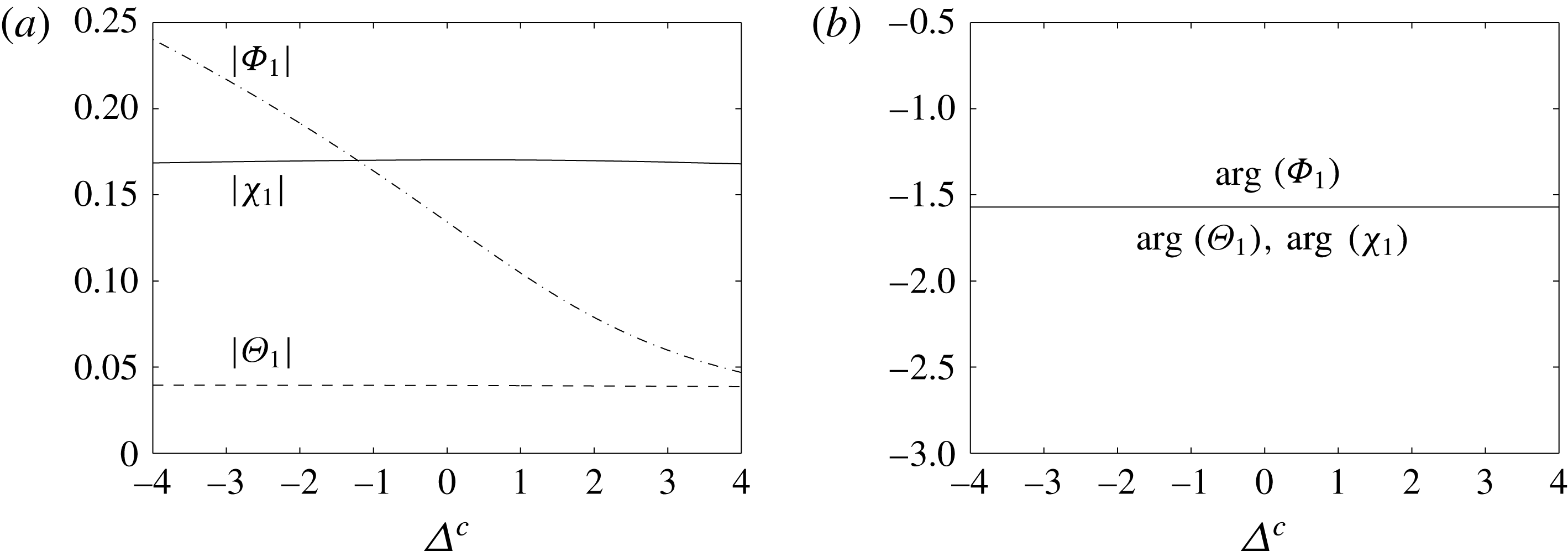
(a) Amplitudes and (b) relative phases of the first harmonics as functions of
 $\unicode[STIX]{x1D6E5}^{c}$
. In (a), the solid line is
 $|\unicode[STIX]{x1D712}_{1}|$
, the dashed line is
 $|\unicode[STIX]{x1D6E9}_{1}|$
and the dashed–dotted line is
 $|\unicode[STIX]{x1D6F7}_{1}|$
. In (b), the solid line is
 $\arg (\unicode[STIX]{x1D712}_{1})$
, the dashed line is
 $\arg (\unicode[STIX]{x1D6E9}_{1})$
and the dashed–dotted line is
 $\arg (\unicode[STIX]{x1D6F7}_{1})$
; the three lines are indistinguishable. The parameter values are
 $\unicode[STIX]{x1D719}_{0}=0.1$
,
 $k_{0}=20$
,
 $\unicode[STIX]{x1D6FF}=-0.1$
,
 $\unicode[STIX]{x1D6FC}=3$
,
 $Le=10$
,
 $\unicode[STIX]{x1D706}=0.25$
,
 ${\mathcal{R}}_{C}=-50$
.

(a) Amplitudes and (b) relative phases of the second harmonics as functions of
 $\unicode[STIX]{x1D6E5}^{c}$
. In (a), the solid line is
 $|\unicode[STIX]{x1D712}_{2}|$
, the dashed line is
 $|\unicode[STIX]{x1D6E9}_{2}|$
, the dashed–dotted line is
 $|\unicode[STIX]{x1D6F7}_{2}|$
and the dotted line is
 $|\unicode[STIX]{x1D713}_{2}|$
. In (b), the solid line is
 $\arg (\unicode[STIX]{x1D712}_{2}/\unicode[STIX]{x1D712}_{1})$
, the dashed line is
 $\arg (\unicode[STIX]{x1D6E9}_{2}/\unicode[STIX]{x1D6E9}_{1})$
, the dashed–dotted line is
 $\arg (\unicode[STIX]{x1D6F7}_{2}/\unicode[STIX]{x1D6F7}_{1})$
and the dotted line is
 $\arg (\unicode[STIX]{x1D713}_{2})$
; each set of lines are practically indistinguishable. The parameter values are
 $\unicode[STIX]{x1D719}_{0}=0.1$
,
 $k_{0}=20$
,
 $\unicode[STIX]{x1D6FF}=-0.1$
,
 $\unicode[STIX]{x1D6FC}=3$
,
 $Le=10$
,
 $\unicode[STIX]{x1D706}=0.25$
,
 ${\mathcal{R}}_{C}=-50$
.

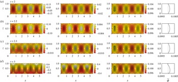
Eigenfunctions from the Galerkin analysis. Left-hand column: streamlines superimposed on the concentration perturbation
 $\tilde{C}$
. Centre column: streamlines superimposed on the temperature perturbation
 $\tilde{T}$
. Right-hand column: streamlines superimposed on the porosity perturbation
 $\tilde{\unicode[STIX]{x1D719}}$
. The parameter values are
 $\unicode[STIX]{x1D719}_{0}=0.1$
,
 $k_{0}=20$
,
 $\unicode[STIX]{x1D6FF}=-0.1$
,
 $\unicode[STIX]{x1D6FC}=3$
,
 $Le=10$
,
 $\unicode[STIX]{x1D706}=0.25$
,
 ${\mathcal{R}}_{C}=-50$
. In each case, the values of
 $\unicode[STIX]{x1D713}$
on the streamlines are evenly spaced, and in each plot, darker shading corresponds to lower values; scales are arbitrary.

Figures 8 and 9 show how the amplitudes and phases of the perturbations to the streamfunction, temperature, concentration and porosity vary as
 $\unicode[STIX]{x1D6E5}^{c}$
changes for
 $k_{0}=20$
,
 ${\mathcal{R}}_{C}=-50$
. They should be read in conjunction with figure 4(a,b), which illustrates the behaviour of
 $\unicode[STIX]{x1D70E}$
with
 $\unicode[STIX]{x1D6E5}^{c}$
, and figure 10, which illustrates how the corresponding spatial structure of the fastest-growing eigenfunction behaves as
 $\unicode[STIX]{x1D6E5}^{c}$
is reduced. It should be recalled that in this case there is no bifurcation point and for all values of
 $\unicode[STIX]{x1D6E5}^{c}$
,
 $\unicode[STIX]{x1D70E}$
is strictly real.
At
 $\unicode[STIX]{x1D6E5}^{c}=3$
, the perturbations to the concentration, temperature and porosity are all small (figure 8
a), and the phase (figure 8
b) is such that the maxima of
 $\tilde{C}$
,
 $\tilde{T}$
and
 $\tilde{\unicode[STIX]{x1D719}}$
all coincide. This is the situation in figure 10
a: downflow draws down lower concentrations and temperatures from the upper boundary, while upflow draws up higher concentrations and temperatures from the lower boundary. Downflow occurs in low-permeability regions and upflow in high-permeability regions.
As
 $\unicode[STIX]{x1D6E5}^{c}$
is reduced, the first harmonic of
 $\tilde{\unicode[STIX]{x1D719}}$
grows in importance, while those of
 $\tilde{C}$
and
 $\tilde{T}$
remain small (figure 8
a), and the second harmonics become more apparent (figure 9
a). Furthermore, the temperature and streamfunction cells are flattened upwards (
 $\arg (\unicode[STIX]{x1D713}_{2})=\arg (\unicode[STIX]{x1D6E9}_{2}/\unicode[STIX]{x1D6E9}_{1})=\unicode[STIX]{x03C0}$
, figure 9
b), and the concentration and porosity cells are flattened downwards (
 $\arg (\unicode[STIX]{x1D712}_{2}/\unicode[STIX]{x1D712}_{1})=\arg (\unicode[STIX]{x1D6F7}_{2}/\unicode[STIX]{x1D6F7}_{1})=0$
, figure 9
b). This flattening of cells can be seen in figure 10(b,c) for
 $\unicode[STIX]{x1D6E5}^{c}=0$
and
 $\unicode[STIX]{x1D6E5}^{c}=-3$
respectively. It should be noted that the amplitudes of the first and second harmonics are much smaller here than in the subcritical case, and hence the distortion of the cells is not as evident as in figure 7(b,c).
The behaviour here is identical to that seen for the subcritical Damköhler number after the abrupt branch switching (
 $\unicode[STIX]{x1D6E5}^{b}<0.4$
). As in that case, vertical convection balances with diffusion in the temperature perturbation equation (3.2), and it balances with the
 $\unicode[STIX]{x2202}\unicode[STIX]{x1D719}^{\prime }/\unicode[STIX]{x2202}z$
term in the concentration perturbation equation (3.3), for all values of
 $\unicode[STIX]{x1D6E5}^{c}$
. This results in an offset between the porosity and circulation cells, which in turn causes the upward movement of the circulation and temperature cells, and downward movement of the porosity and concentration cells.
4 Numerical simulations
To examine the nonlinear behaviour and the effect of flow–permeability feedback over longer time scales, the system was numerically integrated using the finite-element package Comsol Multiphysics v4.2. The two-dimensional equations were solved in a rectangular domain,
 $0<x<10$
,
 $0<z<1$
, and the boundary conditions (2.19) were applied on the horizontal boundaries, while periodicity was imposed on the vertical boundaries. Following Pritchard & Richardson (Reference Pritchard and Richardson2007) and Ritchie & Pritchard (Reference Ritchie and Pritchard2011), we expect this domain to be sufficiently wide for the system to select a preferred wavenumber without strong influence from the imposed periodicity. For all numerical simulations described here, the initial conditions were taken to be
 $$\begin{eqnarray}\displaystyle \left.\begin{array}{@{}c@{}}\displaystyle \tilde{T}(x,z,0)=\tilde{C}(x,z,0)=\unicode[STIX]{x1D716}z(1-z)\sin (\unicode[STIX]{x03C0}x),\\ \displaystyle \unicode[STIX]{x1D719}(x,z,0)=\unicode[STIX]{x1D719}_{0}+10\unicode[STIX]{x1D716}z(1-z)\sin (\unicode[STIX]{x03C0}x),\end{array}\right\} & & \displaystyle\end{eqnarray}$$
where
 $\unicode[STIX]{x1D716}=10^{-3}$
.
A large number of simulations were conducted to verify the convergence and mesh independence of our numerical model, and to validate the model against the linear stability analysis results. Details of these simulations can be found in Corson (Reference Corson2012, § 6.1.1, appendix B.2).
We will consider two different scenarios: first, a destabilising thermal gradient with a stabilising solutal gradient and a subcritical Damköhler number, so that the onset of instability is oscillatory; second, a destabilising thermal gradient with a stabilising solutal gradient and a supercritical Damköhler number, so that the onset of instability is direct. Each simulation we describe uses the parameters
 $\unicode[STIX]{x1D719}_{0}=0.1$
,
 $|\unicode[STIX]{x1D6FF}|=0.001$
,
 $Le=10$
, and
 $\unicode[STIX]{x1D706}=0.25$
. With a subcritical Damköhler number, the simulation lasts
 $2\times 10^{4}$
time units, while with a supercritical Damköhler number, the simulation lasts
 $10^{4}$
time units. For each value of the solutal Rayleigh number
 ${\mathcal{R}}_{C}$
used, we take the corresponding thermal Rayleigh number to be 10 % above its critical value.
Onset of convection for
 ${\mathcal{R}}_{C}=-15$
,
 ${\mathcal{R}}_{T}=299$
and
 $k_{0}=5$
. The shading indicates the solutal concentration perturbation
 $\tilde{C}$
(left), the temperature perturbation
 $\tilde{T}$
(centre) and the porosity
 $\unicode[STIX]{x1D719}$
with its horizontal average
 $\overline{\unicode[STIX]{x1D719}}$
(right). One should note the different magnitudes of
 $\tilde{C}$
,
 $\tilde{T}$
and
 $\unicode[STIX]{x1D719}$
on each subset of plots. The solid lines are streamlines, which correspond to evenly spaced values of the streamfunction in steps of (a,c) 0.04, (b) 0.003 and (d) 1.6. The flow direction is indicated by the arrow at
 $x=0.5$
in the plot of
 $\unicode[STIX]{x1D719}$
.

Evolution for
 ${\mathcal{R}}_{C}=-15$
,
 ${\mathcal{R}}_{T}=299$
and
 $k_{0}=5$
. The shading indicates the solutal concentration perturbation
 $\tilde{C}$
(left), the temperature perturbation
 $\tilde{T}$
(centre) and the porosity
 $\unicode[STIX]{x1D719}$
with its horizontal average
 $\overline{\unicode[STIX]{x1D719}}$
(right). The solid lines in each plot are streamlines, which correspond to evenly spaced values of the streamfunction in steps of 2 at each time. Additional streamlines are plotted with dashed lines. (These correspond to further evenly spaced values of the streamfunction, but the spacing is not the same at each time.) The flow direction is indicated by the arrow at
 $x=0.5$
in the plot of
 $\unicode[STIX]{x1D719}$
.

4.1 Stabilising solutal gradient, destabilising thermal gradient, subcritical Damköhler number
In this and the subsequent subsection, we consider the combination of a stabilising solutal gradient with a destabilising thermal gradient. Here, we consider this combination together with a subcritical Damköhler number; we recall that in this case, the transition to instability is through a growing oscillatory mode.
Figures 11 and 12 show the evolution of the concentration perturbation
 $\tilde{C}$
, the temperature perturbation
 $\tilde{T}$
and the porosity
 $\unicode[STIX]{x1D719}$
for the left half of the domain, for
 ${\mathcal{R}}_{C}=-15$
,
 ${\mathcal{R}}_{T}=299$
and
 $k_{0}=5$
. These figures should be read in conjunction with figure 13(a), which shows the evolution of the maximum absolute velocity and the maximum and minimum porosity within the domain. In figure 11, one should note the different magnitudes of
 $\tilde{C}$
,
 $\tilde{T}$
and
 $\unicode[STIX]{x1D719}$
in each subset of plots. The solid lines in each plot are the streamlines, which correspond to evenly spaced values of the streamfunction in steps of (a,c) 0.04, (b) 0.003 and (d) 1.6. The flow direction is indicated by the arrow at
 $x=0.5$
in the plot of
 $\unicode[STIX]{x1D719}$
.
At
 $t=2$
(figure 11
a), all of the fields are in phase; that is, regions of
 $\tilde{C}>0$
and
 $\tilde{T}>0$
coincide with regions of lower porosity (
 $\unicode[STIX]{x1D719}<\unicode[STIX]{x1D719}_{0}$
), and regions of
 $\tilde{C}<0$
and
 $\tilde{T}<0$
coincide with regions of higher porosity (
 $\unicode[STIX]{x1D719}>\unicode[STIX]{x1D719}_{0}$
). At this time, we have upward flow in
 $\tilde{C}>0$
and
 $\tilde{T}>0$
regions, and downward flow in
 $\tilde{C}<0$
and
 $\tilde{T}<0$
regions. However, by
 $t=2.2$
(figure 11
b), the flow direction has switched, but the concentration, temperature and porosity fields have remained in phase. The concentration and temperature fields move a half-cell by
 $t=2.3$
(figure 11
c), so again we have upward flow in
 $\tilde{C}>0$
and
 $\tilde{T}>0$
regions, but now the concentration and temperature fields are out of phase with the porosity field. The fields remain out of phase, and by
 $t=3$
(figure 11
d), nonlinear effects have become significant, as seen by the plumes of high- and low-concentration perturbations.
The oscillatory onset can also be seen in the inset of figure 13(a). We can see that the maximum velocity grows as convection tries to establish itself, but then drops as the flow direction changes. This occurs twice before the phase shift at
 $t=2.3$
, after which the velocity grows rapidly as convection develops.
Since nonlinear effects enter the system so rapidly, there is not a chance to see the upward movement of the circulation and temperature fields and downward movement of the concentration and porosity fields predicted by the two-term Galerkin approximation to the linear stability analysis. However, the concentration and temperature fields are out of phase with the porosity field, as predicted.
Maximum absolute velocity
 $|\boldsymbol{u}|$
(solid) and maximum and minimum porosity
 $\unicode[STIX]{x1D719}$
(dashed) throughout the whole domain for (a)
 $k_{0}=5$
,
 ${\mathcal{R}}_{C}=-15$
,
 ${\mathcal{R}}_{T}=299$
; (b)
 $k_{0}=20$
,
 ${\mathcal{R}}_{C}=-15$
,
 ${\mathcal{R}}_{T}=245$
.

Figure 12 shows the evolution of the concentration perturbation
 $\tilde{C}$
, temperature perturbation
 $\tilde{T}$
and porosity
 $\unicode[STIX]{x1D719}$
for the left half of the domain. The solid lines in each plot are streamlines, which correspond to evenly spaced values of the streamfunction in steps of 2 at each time. To aid with the visualisation of the flow, additional streamlines are plotted with dashed lines. (These correspond to further evenly spaced values of the streamfunction, but the spacing is not the same at each time.) The flow direction is indicated by the arrow at
 $x=0.5$
in the plot of
 $\unicode[STIX]{x1D719}$
. Figure 12 should be read in conjunction with figure 13(a), which shows the evolution of the maximum absolute velocity, and the maximum and minimum porosity.
At
 $t=100$
(figure 12
a), the concentration and temperature fields are very similar to those at the onset of convection (
 $t=3$
, figure 11
d), but the porosity field has begun to evolve, with porosity increasing where
 $\tilde{C}<0$
and
 $\tilde{T}<0$
and decreasing where
 $\tilde{C}>0$
and
 $\tilde{T}>0$
. Therefore, the porosity is reduced slightly near the top of the layer, and correspondingly the centres of the circulation cells have moved down towards the bottom of the layer. This region of reduced porosity is pierced by higher-porosity channels which correspond with the downflow regions of the circulation. Here, downflow is faster than upflow, as seen by the more tightly packed streamlines.
The porosity continues to evolve and by
 $t=500$
(figure 12
b), the region of lower porosity at the top of the domain has extended downwards, flattening the circulation cells even more. High-porosity channels still pierce the low-porosity region in areas of downward flow, but now upflow under the low-porosity barrier is faster than downflow.
Figure 13(a) shows the evolution of the maximum absolute velocity, and we can see that convection is established and maintained until
 $t\approx 750$
, when the porosity evolution has forced the circulation into too small a region to be maintained (figure 12
c). We then enter a regime of slow porosity evolution, which strives to reach a state where convection can be maintained again.
At
 $t=1000$
(figure 12
d), the circulation is still contained in the lower half of the domain, but additional counter-rotating cells have formed in the high-porosity region at the bottom of the channels. By
 $t=5000$
(figure 12
e), these new circulation cells have expanded upwards and now extend the full height of the domain, confining the original circulation cells even more strongly to the bottom of the domain. It should be noted that further pairs of counter-rotating circulation cells have formed at the top of the domain at the top of the high-porosity channel, and by
 $t=10\,000$
(figure 12
f), these circulation cells have started to dominate the flow.
From the maximum-porosity curve in figure 13(a), we can split the slow-evolution regime into two periods: one in which the maximum porosity decreases (
 $t\approx 750$
–10 000) and one in which it increases (
 $t\approx 10\,000$
–18 000). These periods correspond to times when the system is dominated by faster upflow and faster downflow respectively.
By
 $t=15\,000$
(figure 12
g), the new circulation cells have extended to cover most of the domain and the high-porosity channel is now more evident. This channel continues to be eroded (
 $t=17\,500$
, figure 12
h) until vigorous convection can be re-established (
 $t=17\,600$
, figure 12
i). The downward movement of the circulation cells continues, however, and by the end of the simulation (
 $t=20\,000$
, figure 12
j), the very vigorous convection is localised in high-porosity regions near the bottom of the domain (note the different scale on the porosity plot).
The maximum porosities of
 $\unicode[STIX]{x1D719}=0.8$
observed at the end of this simulation may not be physically realistic in the context of naturally occurring porous media, where
 $\unicode[STIX]{x1D719}$
rarely exceeds 0.6 (Nield & Bejan Reference Nield and Bejan2006, § 1.2). At such high porosities, extensions of Darcy’s law (such as the Brinkman equation) would be required (Nield & Bejan Reference Nield and Bejan2006, § 1.5). This high porosity is a result of our assumption that the porous medium is entirely soluble. We would expect a more complete model to predict lower maximum porosities; however, our results strongly suggest that even in such a model, complete depletion of the soluble component from parts of the rock matrix may be expected.
Evolution for
 ${\mathcal{R}}_{C}=-15$
,
 ${\mathcal{R}}_{T}=245$
and
 $k_{0}=20$
. The shading indicates the solutal concentration perturbation
 $\tilde{C}$
(left), the temperature perturbation
 $\tilde{T}$
(centre) and the porosity
 $\unicode[STIX]{x1D719}$
with its horizontal average
 $\overline{\unicode[STIX]{x1D719}}$
(right). The solid lines in each plot are streamlines, which correspond to evenly spaced values of the streamfunction in steps of 1 at each time. Additional streamlines are plotted with dashed lines. (These correspond to further evenly spaced values of the streamfunction, but the spacing is not the same at each time.) The flow direction is indicated by the arrow at
 $x=0.5$
in the plot of
 $\unicode[STIX]{x1D719}$
.

4.2 Stabilising solutal gradient, destabilising thermal gradient, supercritical Damköhler number
We now consider the combination of a stabilising solutal gradient with a destabilising thermal gradient together with a supercritical Damköhler number, so that the transition to instability is direct. Figure 14 shows the evolution of the concentration perturbation
 $\tilde{C}$
, temperature perturbation
 $\tilde{T}$
and porosity
 $\unicode[STIX]{x1D719}$
for the left half of the domain, for
 ${\mathcal{R}}_{C}=-15$
,
 ${\mathcal{R}}_{T}=245$
and
 $k_{0}=20$
. The solid lines in each plot are streamlines, which correspond to evenly spaced values of the streamfunction in steps of 1 at each time. To aid with the visualisation of the flow, additional streamlines are plotted with dashed lines. (These correspond to further evenly spaced values of the streamfunction, but the spacing is not the same at each time.) The flow direction is indicated by the arrow at
 $x=0.5$
in the plot of
 $\unicode[STIX]{x1D719}$
. Figure 14 should be read in conjunction with figure 13(b), which shows the evolution of the maximum absolute velocity, and the maximum and minimum porosity.
Convection is apparent by
 $t\approx 2$
(not shown). At this time, the fields are out of phase, with regions of
 $\tilde{C}>0$
and
 $\tilde{T}>0$
coinciding with regions of higher porosity (
 $\unicode[STIX]{x1D719}>\unicode[STIX]{x1D719}_{0}$
), and regions of
 $\tilde{C}<0$
and
 $\tilde{T}<0$
coinciding with regions of lower porosity (
 $\unicode[STIX]{x1D719}<\unicode[STIX]{x1D719}_{0}$
). Once convection has been established, the flow very quickly becomes dominated by nonlinear effects. Therefore, as in the subcritical case, there is no chance to see the vertical displacement predicted by the Galerkin analysis. However, the concentration and temperature fields are out of phase with the porosity field, as predicted.
Since the diffusion of solute is much slower than the diffusion of heat, the concentration perturbations are advected with the flow. This is the picture that has emerged by
 $t=100$
(figure 14
a), when we see plumes of low concentration being drawn towards the bottom of the domain, and those of high concentration being drawn towards the top of the domain, by the circulation. The porosity field continues to evolve, with porosity increasing in regions that coincide with
 $\tilde{C}<0$
and
 $\tilde{T}<0$
, and decreasing in regions that coincide with
 $\tilde{C}>0$
and
 $\tilde{T}>0$
. Therefore, the porosity is reduced near the top of the layer, and correspondingly the centres of the circulation cells have moved downwards. However, this region of low porosity is pierced by higher-porosity channels in which fluid is carried towards the bottom of the layer. Furthermore, downflow is faster than upflow, as can be seen by the more tightly packed streamlines in these regions.
From figure 13(b), we can see that the maximum velocity increases as convection is established, and then suddenly convection is halted at
 $t\approx 130$
. During this time, the porosity contrast has increased substantially (figure 13
b), but once convection is halted, we enter a regime of slow porosity evolution. This is identical behaviour to that seen for a subcritical Damköhler number in § 4.1, although in this case the period of vigorous convection is much shorter.
Figure 14(b) shows the fields at
 $t=130$
just as the convection is halted. By this time, both the concentration and the temperature perturbations are greatly reduced, and, although the porosity field looks similar to that at
 $t=100$
, the porosity contrast between the regions of high and low porosity has increased. As a result of the region of low porosity extending across the top half of the domain, the circulation has been confined closer to the bottom of the layer. Consequently, the vigorous convection cannot continue, resulting in this much slower circulation.
By
 $t=500$
(figure 14
c), the circulation has been confined even closer to the bottom of the domain, and there is now no circulation in the top half of the domain. Small additional circulation cells have appeared at the bottom of the domain in the high-porosity regions, and these grow in size (
 $t=1000$
, figure 14
d), until by
 $t=2000$
(figure 14
e), they extend the full height of the domain. It should be noted that throughout this evolution, the region of high porosity at the bottom of the layer has become thinner, so now most of the layer is dominated by lower porosity. However, channels of slightly higher porosity still pierce the domain, but these now contain fluid moving upwards towards the top of the domain. Furthermore, the top of each channel now contains a pair of counter-rotating circulation cells.
By
 $t=5000$
(figure 14
f), the circulation cells that appeared at the top of the higher-porosity channels have increased in size, and, in the region of downflow, the porosity has increased. These circulation cells continue to expand downwards while the lower cells shrink (figure 14
g), until by
 $t=7000$
(figure 14
h), the upper cells almost fill the domain.
From the maximum-porosity curve in figure 13(b), we can see that the slow evolution can be split into three regions: from
 $t\approx 130$
–2000 the maximum porosity remains constant, then from
 $t\approx 2000$
–6000 it decreases, before increasing again from
 $t\approx 6000$
. These regions correspond to periods during which the system is dominated by faster downflow in high-porosity regions, then faster upflow, and finally faster downflow respectively. A similar pattern was seen in § 4.1 for a subcritical Damköhler number.
By
 $t=9000$
(figure 14
i), the centres of the circulation cells have moved downwards, and the porosity has increased further in the downflow channel. The porosity continues to increase until, by
 $t=10\,000$
(figure 14
j), vigorous convection is able to return.
5 Summary and conclusions
We have investigated the behaviour of a mathematical model of thermosolutal convection in a saturated porous layer, when the solubility of the solute depends on the temperature, and the porosity and permeability of the porous medium evolve through dissolution and precipitation. When the solutal concentration gradient is destabilising, the dynamics resemble those previously found for single-species convection (Ritchie & Pritchard Reference Ritchie and Pritchard2011), including the occurrence of subcritical instabilities driven by a reaction–diffusion mechanism. This suggests that the single-species model of Ritchie & Pritchard (Reference Ritchie and Pritchard2011) captures the fundamental feedback mechanisms that drive the evolution of the rock matrix in solutally driven convection.
When the solutal concentration gradient is stabilising and the thermal gradient is destabilising, novel dynamics emerge. Here, the Damköhler number
 $k_{0}$
plays an important role at the onset of convection, with slow dissolution and precipitation (lower
 $k_{0}$
) leading to an oscillatory instability, but faster dissolution and precipitation (higher
 $k_{0}$
) leading to a monotonic instability. Instead of the tilted cells and lateral movement seen in the solutally unstable case, the cells in this case are displaced vertically, with the porosity and concentration cells being flattened towards the bottom of the layer, while the circulation and temperature cells are flattened towards the top of the layer (figure 7).
Over longer time scales, although quasi-steady convective circulation is established initially, the porosity evolution triggers an interaction between processes operating at different time scales (figures 12 and 14). Over dimensionless time scales of order 100, the reinforcement of the in-phase porosity structure confines the circulation within too small a region for it to be maintained. Once convection is suppressed, a slow porosity evolution occurs over dimensionless time scales of order 1000, resulting in a layered porosity structure penetrated by high-permeability channels. There is an almost continual vertical movement of the circulation cells, but eventually the porosity evolves sufficiently to allow the return of very vigorous localised convection in regions of high porosity.
With a dominant thermal gradient, the porosity evolution plays apparently contradictory roles: suppressing the convective instability over medium time scales, but allowing the resurgence of convection as the porosity increases locally over very long time scales. This resurgence of convection highlights the importance of running numerical simulations for a sufficiently long time, since our results (e.g. figure 13 b) suggest that vigorous convective circulation can return even after very long quiescent periods.
There are many opportunities for further studies to explore whether our findings are robust to increased model complexity. Promising directions would be to consider more detailed models of the geochemistry (Bolton et al. Reference Bolton, Lasaga and Rye1996, Reference Bolton, Lasaga and Rye1997, Reference Bolton, Lasaga and Rye1999; Weis Reference Weis2015), including multiple species and reaction between them, and to allow the porous matrix to contain insoluble as well as soluble material (Ward et al. Reference Ward, Jensen, Power and Riley2015; Petrus & Szymczak Reference Petrus and Szymczak2016). While we would expect the detailed behaviour of such systems to differ from that described here, the present study has illustrated how interacting processes with very different time scales can generate inhomogeneity and thus strongly localised dynamics in even the simplest systems in which buoyancy-driven flow drives the evolution of a porous medium.
Acknowledgements
We are grateful to Professors M. G. Worster and N. J. Mottram for valuable discussions, and to three anonymous referees for their detailed and constructive comments. L.T.C. was supported by a scholarship (2009–2012) from the Carnegie Trust for the Universities of Scotland.