
1. Introduction
The Stokes layer is the flow established by the sinusoidal motion of an infinitely long bounding flat plate beneath an otherwise stationary body of fluid. This unsteady flow yields one of the few known exact solutions to the Navier–Stokes equations, and so is the archetype model for investigating stability behaviour in temporally periodic flows. Given the periodicity of the underlying basic state, the stability problem naturally lends itself to Floquet analysis, whereby the net growth (or decay) of linear disturbances is determined over each full cycle of wall oscillation.
The Floquet approach accounts for the periodicity of the unsteady flow by assuming that disturbances are decomposed into modes with a time dependency of the form  $\exp (\mu t)p(t)$, where
 $p$ is a time-periodic function with the same period as the basic state. The net growth of the disturbance is then encompassed in the real part of the Floquet exponent
 $\mu$. Perturbation equations are derived from the Navier–Stokes equations in a manner analogous to the derivation of the Orr–Sommerfeld equation (that governs the stability of steady flows).
1.1. General background
Floquet theory was first formulated for the Stokes layer by Hall (Reference Hall1978), who showed that the flow is linearly stable for Reynolds numbers  ${Re} < 160$ – a formal definition for the Reynolds number
 ${Re}$ is given below in (2.3). Following the advancement of computational technology, Blennerhassett & Bassom (Reference Blennerhassett and Bassom2002) extended the Floquet analysis to significantly larger values of
 ${Re}$, wherein a section of the neutral stability curve was traced and it was determined that linearly unstable behaviour emerges for the critical Reynolds number
 ${Re}_c = 707.84$. Equivalent formulations were subsequently used to investigate the linear stability of related flows, such as the finite Stokes layer in channels and pipes (Blennerhassett & Bassom Reference Blennerhassett and Bassom2006; Thomas et al. Reference Thomas, Bassom, Blennerhassett and Davies2011; Thomas, Bassom & Blennerhassett Reference Thomas, Bassom and Blennerhassett2012).
Informed by the results of these earlier studies, Thomas et al. (Reference Thomas, Davies, Bassom and Blennerhassett2014) carried out direct numerical simulations (DNS) of the linearised Navier–Stokes equations to explore the impulse response of disturbances in the semi-infinite Stokes layer. Numerical simulations revealed an intriguing spatio-temporal formation that was described as a family-tree structure, which involves the successive birthing of distinct wavepackets. Moreover, it was demonstrated that DNS calculations were in excellent agreement with the Floquet stability analysis, despite computational restrictions limiting DNS to the first three periods of wall motion.
Although agreement between linear stability analysis and DNS was demonstrated, experiments on the Stokes layer generally observe unstable behaviour and transition to turbulence for Reynolds numbers  ${Re}<300$ (Hino, Sawamoto & Takasu Reference Hino, Sawamoto and Takasu1976; Clamen & Minton Reference Clamen and Minton1977; Akhaven, Kamm & Shapiro Reference Akhaven, Kamm and Shapiro1991; Eckmann & Grotberg Reference Eckmann and Grotberg1991), which is significantly lower than the Floquet predictions (Blennerhassett & Bassom Reference Blennerhassett and Bassom2002). In an attempt to address the significant differences between theory and experiments, it was noted by Thomas et al. (Reference Thomas, Blennerhassett, Bassom and Davies2015) that many experiments report some noise associated with the mechanical oscillation of the bounding plate. Naturally, it is difficult to retroactively determine the level of noise in experiments, but many experimentalists quote a noise amplitude of
 $1\,\%$ of the fundamental oscillation. Based on this observation, Thomas et al. (Reference Thomas, Blennerhassett, Bassom and Davies2015) undertook a stability investigation of the Stokes layer subject to a low-amplitude, high-frequency harmonic. It was shown that the introduction of this form of modulation brought about a dramatic destabilisation of the flow, bringing the critical Reynolds number
 ${Re}_c$ for unstable behaviour in line with experimental observations. While the form of these high-frequency harmonics is not particularly comparable to the supposedly random noise observed in experiments, the considerable reduction in
 ${Re}_c$ suggests that the presence of noise can have a significant effect on the stability of the flow.
This investigation follows the recent work by Ramage et al. (Reference Ramage, Davies, Thomas and Togneri2020) in which disturbance development was successfully simulated for 20 periods of wall motion for both the classical Stokes layer and several cases where the basic state was modified via a high-frequency, low-amplitude harmonic. The longer time numerical simulations suggest that the Stokes layer is subject to an absolute form rather than a convective form of instability. Convective instability describes an unstable disturbance that propagates along one direction only, while absolute instability is characterised by growth at every spatial location.
1.2. Key features of the disturbance development
In order to fully contextualise the present investigation, we describe the key observations of Ramage et al. (Reference Ramage, Davies, Thomas and Togneri2020) that will be explored further herein.
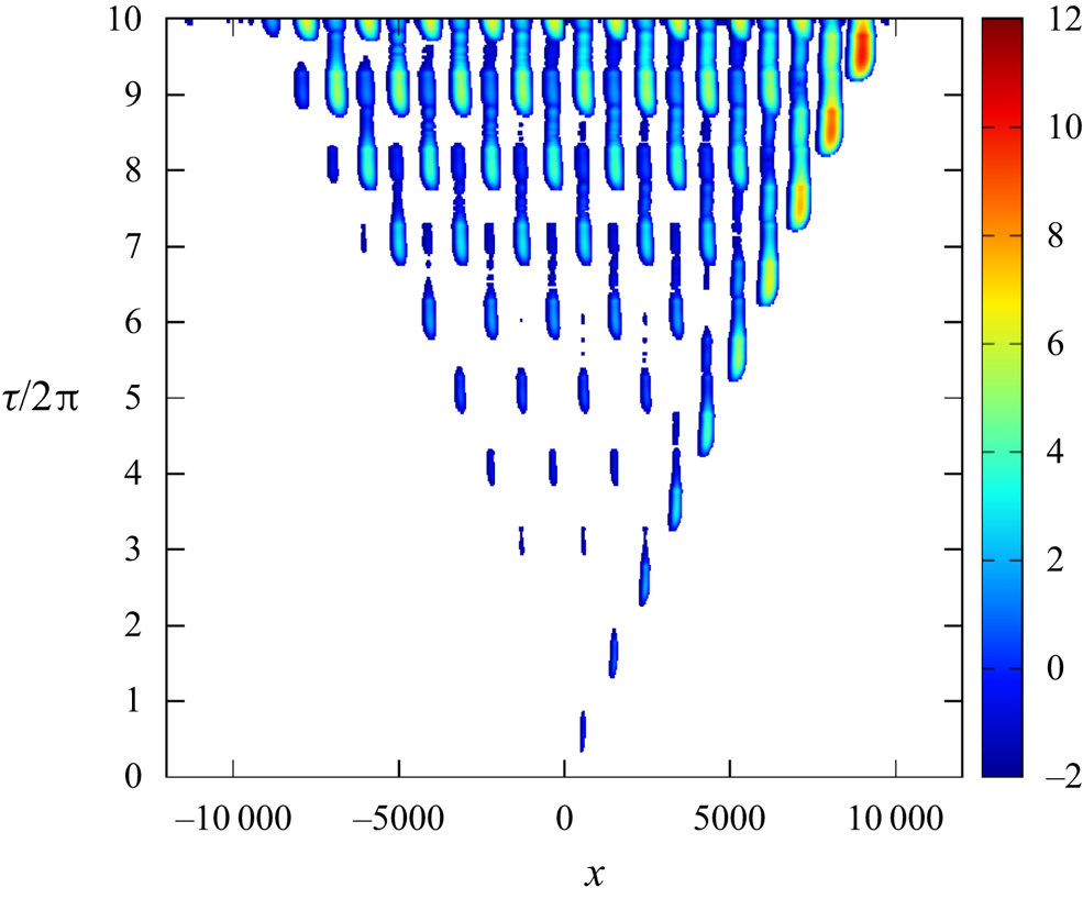
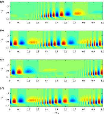
Figure 1 is a reproduction of figure 3 of Ramage et al. (Reference Ramage, Davies, Thomas and Togneri2020) and displays the impulse response of the linear disturbance in the Stokes layer at the Reynolds number  ${Re} = 750$. Contours are based on the logarithm of the absolute value of the wall vorticity perturbation. This plot is included here to illustrate the spatio-temporal development of the family-tree structure, first reported in Thomas et al. (Reference Thomas, Davies, Bassom and Blennerhassett2014), and highlight the key features of the disturbance evolution. For details on the generation of this plot, the interested reader is directed to Ramage et al. (Reference Ramage, Davies, Thomas and Togneri2020). Here, it is sufficient to state that the respective contours indicate the magnitude of the disturbance as a function of the streamwise
 $x$-direction (in which the plate oscillates) and the non-dimensional time
 $\tau /2{\rm \pi}$ (the number of plate oscillations).
Reproduction of figure 3 from Ramage et al. (Reference Ramage, Davies, Thomas and Togneri2020). Spatio-temporal contour plot of the linear disturbance in the Stokes layer with  ${Re} = 750$. Contours are based on the logarithm of the absolute value of the wall vorticity perturbation.

At time  $\tau =0$, the initial impulse excites a disturbance wavepacket that convects to the right. This initial wavepacket is called the mother wavepacket. Within each period of the wall oscillation, two daughter wavepackets are birthed that propagate to the left and right of the original mother wavepacket. (In the early stages of the disturbance evolution, these particular wavepackets develop at magnitudes below the low-amplitude cutoff and do not appear in the contour plot depicted in figure 1. However, they do become more obvious at later times, when the disturbance achieves larger amplitudes.) The daughter wavepackets then birth granddaughter wavepackets and so on, giving rise to the so-called family-tree structure shown in figure 1.
It is immediately obvious from figure 1 that the disturbance maximum convects along those wavepackets located on the right-hand side of the illustration. Moreover, the growth rate associated with the disturbance maximum was found by Ramage et al. (Reference Ramage, Davies, Thomas and Togneri2020) to match the growth rate determined via Floquet stability theory (Blennerhassett & Bassom Reference Blennerhassett and Bassom2002).
Pointwise growth of the disturbance is then observed by selecting a single streamwise  $x$-location and tracing the disturbance development over time, i.e. a vertical line in figure 1. Clearly the magnitude of the disturbance, about fixed spatial positions, increases with increasing time. Though it is not evident from this plot alone, it was reported in Ramage et al. (Reference Ramage, Davies, Thomas and Togneri2020) that the growth rate associated with a fixed streamwise
 $x$-location is equal to (or at least remarkably close to) the growth rate of the disturbance maximum, for all Reynolds numbers modelled. This suggests that the Stokes layer is subject to absolutely unstable behaviour, for which the onset coincides with the critical Reynolds number
 ${Re}_c = 707.84$ for linear instability (Blennerhassett & Bassom Reference Blennerhassett and Bassom2002).
A second observation, drawn by Ramage et al. (Reference Ramage, Davies, Thomas and Togneri2020), is the staggered structure of the wavepacket formations. With the passing of each period of wall motion (i.e. time  $\tau /2{\rm \pi}$ is increased by one), the location of each wavepacket is shifted horizontally along the streamwise
 $x$-direction, before returning to their original locations during the next cycle. Thus, at fixed spatial locations, the disturbance structure reasserts itself every two cycles of wall motion. Hence, pointwise evolution is characterised by a subharmonic temporal growth, with a periodicity that is twice that of the basic state.
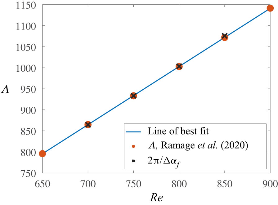
Ramage et al. (Reference Ramage, Davies, Thomas and Togneri2020) also reported that the spacing  $\varLambda$ between the respective mother and daughter wavepackets is fixed and related to the Reynolds number
 ${Re}$. Moreover, due to the staggered nature of the family-tree formation, the distance between two adjacent wavepackets of commensurate size is twice the wavepacket spacing
 $\varLambda$. Thus, the family-tree structure has a spatial periodicity of
 $2\varLambda$.
1.3. Paper objective
Although the numerical investigation by Ramage et al. (Reference Ramage, Davies, Thomas and Togneri2020) strongly suggests that linear disturbances in the Stokes layer are absolutely unstable for Reynolds numbers  ${Re}\geq {Re}_c$, the existence of such behaviour can only be confirmed and understood by undertaking a full theoretical study. This is achieved using a modified form of the Briggs (Reference Briggs1964) method, based on the formulation of Brevdo & Bridges (Reference Brevdo and Bridges1997).
The Briggs method for locating absolutely unstable behaviour is well established for steady flows, such as that on a rotating disc (Lingwood Reference Lingwood1995, Reference Lingwood1997b), while Pier (Reference Pier2003) and Hwang, Kim & Choi (Reference Hwang, Kim and Choi2013) have coupled this approach with Floquet theory to study secondary instabilities on a rotating disc and in a two-dimensional wake, respectively. However, application of these routines to temporally periodic flows has not, to the authors knowledge, been attempted previously. It will be demonstrated that this analysis provides confirmation of the disturbance behaviour reported in Ramage et al. (Reference Ramage, Davies, Thomas and Togneri2020). Moreover, we will:
(i) Determine necessary symmetry constraints for absolute instability, based on the antiperiodicity of the Stokes layer.
(ii) Provide conclusive evidence for the existence of absolutely unstable behaviour in the Stokes layer.
(iii) Determine the mechanisms responsible for establishing absolute instability and explain why pointwise growth is characterised by subharmonic behaviour.
(iv) Formulate a relationship between the spatial periodicity
 $2\varLambda$ of the family-tree structure and the decomposition of the linear disturbance wave spectra.

1.4. Paper structure
The remainder of this paper is outlined as follows. The basic state and non-dimensionalisa- tion are discussed in § 2, followed by the formulation for Floquet stability theory in § 3. In § 4, the Briggs method is introduced and discussed, with the derivation of an integral solution in § 4.1, the development of pinch points in § 4.2 and symmetry arguments in § 4.3. In § 5, results are discussed for the Stokes layer, demonstrating agreement with the symmetry constraints and providing insight into the key features described in § 1.2. Finally, conclusions and suggestions for future work are presented in § 6.
2. Base flow
Although we are primarily interested in the stability of linear disturbances in the semi-infinite Stokes layer, the subsequent modelling is carried out in a two-dimensional channel, as it was shown by Blennerhassett & Bassom (Reference Blennerhassett and Bassom2006) that disturbance behaviour in a sufficiently wide channel is almost identical to that found in the semi-infinite configuration. Moreover, the finite domain is a more natural setting for the spectral numerical methods implemented herein.
Consider the two-dimensional flow of a viscous, incompressible fluid that is bounded between two infinite parallel plates, located a distance  $2d$ apart. Each plate oscillates sinusoidally along the dimensional
 $x^*$-direction with a velocity
 \begin{equation} U_w = U_s \cos(\omega t), \end{equation}
for a frequency of oscillation  $\omega$ and velocity amplitude
 $U_s$. The motion of the bounding plates establishes a uni-directional flow that moves back and forth.
A non-dimensional basic state is obtained by defining the rescaled time  $\tau =\omega t$, while units of velocity and length are scaled on
 $U_s$ and the Stokes layer thickness
 $\delta =\sqrt {2\nu /\omega }$, respectively. Hence, if
 $y$ denotes the direction normal to the bounding surfaces, the non-dimensional base flow is given as
 \begin{equation} \boldsymbol{U} = (U_B(y,\tau),0), \end{equation}
where
 \begin{equation} U_B(y,\tau) = \mbox{Re} \left[\frac{\mathrm{cosh}((1+\textrm{i})y)}{\mathrm{cosh}((1+\textrm{i})h)}\,\mathrm{e}^{\textrm{i}\tau}\right] = u_1\ \textrm{e}^{\textrm{i}\tau}+\bar{u}_{1}\ \textrm{e}^{-\textrm{i}\tau}. \end{equation}
Here,  $h=d/\delta$ is the non-dimensional channel half-width, with
 $h=16$ for the subsequent investigation (the semi-infinite configuration is well approximated when
 $h > 14$, Blennerhassett & Bassom Reference Blennerhassett and Bassom2006; Thomas et al. Reference Thomas, Blennerhassett, Bassom and Davies2015). Additionally, the Reynolds number of the flow is defined as
 \begin{equation} {Re} = \frac{U_s}{\sqrt{2 \nu \omega}}, \end{equation}
where  $\nu$ denotes the kinematic viscosity of the fluid.
The basic state (2.2) is periodic in time with a period of  $2 {\rm \pi}$, i.e.
 $U_B(y,\tau +2{\rm \pi} ) = U_B(y,\tau )$. Moreover, the flow is antiperiodic, meaning that a time shift of half a period corresponds to an exact reversal of the flow, i.e.
 $U_B(y,\tau +{\rm \pi} ) = - U_B(y,\tau )$.
3. Floquet theory
As Squire's theorem has been extended to unsteady flows (Conrad & Criminale Reference Conrad and Criminale1965; Von Kerczek & Davis Reference Von Kerczek and Davis1974), the following analysis is restricted to the development of two-dimensional disturbances. Thus, the total velocity field is given as
 \begin{equation} (u,v) = (U_B,0) + \epsilon \left( \frac{\partial \varPsi}{\partial y}, -\frac{\partial \varPsi}{\partial x} \right), \end{equation}
where  $\epsilon \ll 1$ and
 $\varPsi$ denotes the streamfunction that is decomposed as a Floquet mode
 \begin{equation} \varPsi(x,y,\tau) = \psi(y,\tau)\exp(\mu\tau + \textrm{i}\alpha x) + \textrm{complex conjugate}. \end{equation}
Here,  $\psi (y,\tau )$ is a
 $2{\rm \pi}$-periodic function in time, while
 $\alpha \in \mathbb {R}$ and
 $\mu \in \mathbb {C}$ denote the wavenumber and Floquet exponent, respectively. The growth or decay of the disturbance is included in the real part of
 $\mu$ and, since
 $\psi$ is
 $2{\rm \pi}$-periodic, the disturbance is rescaled by the Floquet multiplier
 $\exp (2 {\rm \pi}\mu )$ after each full period of wall motion.
On substituting (3.1) into the Navier–Stokes equations and linearising in  $\epsilon$, the following governing equation for
 $\psi$ is derived
 \begin{equation} \frac{\partial}{\partial \tau} \mathcal{L} \psi = \left[ \tfrac{1}{2} \mathcal{L} - \mu - \textrm{i} \alpha {Re} U_B \right] \mathcal{L} \psi + \textrm{i} \alpha {Re} U_B'' \psi, \end{equation}
with boundary conditions
 \begin{equation} \psi = \psi' = 0 \quad \textrm{on}\ y={\pm} h, \end{equation}
where a prime denotes differentiation with respect to  $y$ and
 \begin{equation} \mathcal{L} = \frac{\partial^2}{\partial y^2} - \alpha^2. \end{equation}
Perturbations  $\psi$ are then decomposed into harmonics
 \begin{equation} \psi(y,\tau) = \sum_{n={-}\infty}^{\infty} \psi_n(y) \exp(\textrm{i} n \tau), \end{equation}
so that equating coefficients of harmonics in (3.3) results in an infinite system of equations
 \begin{align} \left(\mathcal{L} - \alpha^2 - 2\left(\mu +\textrm{i} n\right)\right) \mathcal{L} \psi_n = \textrm{i} \alpha {Re} \left( u_1 \left(\mathcal{L} \psi_{n-1} - 2 i \psi_{n-1}\right) + \bar{u}_1 \left(\mathcal{L} \psi_{n+1} + 2 \textrm{i} \psi_{n+1}\right)\right). \end{align}
Given the normal mode form (3.2) and Fourier decomposition (3.5), the imaginary part of the Fourier exponent  $\mu$ can be restricted to the interval
 $\mu \in [0,0.5]$. Firstly, if
 $\mu$ is a solution, then so is
 $\mu +\textrm {i}k$ for
 $k\in \mathbb {Z}$. Secondly, due to the symmetry of the Stokes layer, Floquet modes occur as a complex conjugate pair
 $\mu =\mu _r\pm \mu _i$ that are matched to left- and right-travelling waves with equal growth. Moreover, disturbances are stationary in the instance the imaginary part of the Floquet exponent is zero, i.e.
 $\mu _i=0$.
The system of (3.6) can be solved numerically using the pseudospectral techniques described by Trefethen (Reference Trefethen2000). Differential operators (that appear up to fourth order) are replaced by pseudospectral matrix approximations with each  $\psi _n(y)$ replaced by a vector
 $\boldsymbol {\psi }_n$ of its function values on a Chebyshev mesh over the interval
 $-h \leq y \leq h$. Introducing matrix operators
 \begin{equation} \mathcal{L}\rightarrow{\boldsymbol{\mathsf{L}}},\quad \mathcal{L}^2/2\rightarrow {\boldsymbol{\mathsf{V}}} \quad \textrm{and} \quad {\boldsymbol{\mathsf{P}}}={\boldsymbol{\mathsf{L}}}^{{-}1}u_1({\boldsymbol{\mathsf{L}}}-2\textrm{i}{\boldsymbol{\mathsf{I}}}), \end{equation}
allows (3.6) to be rearranged as
 \begin{equation} -\textrm{i}\alpha{Re}\bar{{\boldsymbol{\mathsf{P}}}}\boldsymbol{\psi}_{n+1} +({\boldsymbol{\mathsf{L}}}^{{-}1}{\boldsymbol{\mathsf{V}}}-\textrm{i}n{\boldsymbol{\mathsf{I}}})\boldsymbol{\psi}_{n} -\textrm{i}\alpha{Re}{\boldsymbol{\mathsf{P}}}\boldsymbol{\psi}_{n-1}=\mu\boldsymbol{\psi}_{n}, \end{equation}
where  ${\boldsymbol{\mathsf{I}}}$ is the identity matrix and
 $\bar {{\boldsymbol{\mathsf{P}}}}$ is the complex conjugate of
 ${\boldsymbol{\mathsf{P}}}$.
A finite system of equations is obtained by truncating the Fourier series (3.5), setting  $\psi _n = 0$ for all
 $|n| > N$. The system of equations can then be written in a compact form by the concatenation of
 $\boldsymbol {\psi }_n$ into the vector
 \begin{equation} \boldsymbol{\phi}^{\textrm{T}} = \left( \boldsymbol{\psi}_{N}^{\textrm{T}}, \boldsymbol{\psi}_{N-1}^{\textrm{T}}, \ldots, \boldsymbol{\psi}_{0}^{\textrm{T}}, \ldots, \boldsymbol{\psi}_{{-}N}^{\textrm{T}} \right). \end{equation}
In this manner, the problem is reduced to the eigenvalue problem
 \begin{equation} {\boldsymbol{\mathsf{A}}} \boldsymbol{\phi} = \mu \boldsymbol{\phi}, \end{equation}
where  ${\boldsymbol{\mathsf{A}}}$ is a block-tridiagonal matrix (with block size defined via the Chebyshev discretisation).
The number of harmonics  $N$ was carefully chosen to ensure that results were unchanged by further increases in
 $N$. In many cases
 $N=300$ harmonics were necessary, while sufficient resolution along the wall-normal
 $y$-direction was achieved by using
 $100$ Chebyshev points, resulting in a prohibitively large system (3.10). However, the least-stable disturbances are expected to be symmetric about the channel centre (as per Blennerhassett & Bassom Reference Blennerhassett and Bassom2006). Thus, the size of the system can be significantly reduced by considering only even Chebyshev functions. Finally, since the block-tridiagonal matrix contains mostly zeros, the eigenvalue problem is efficiently solved using the sparse matrix eigenvalue routine in Matlab. Further details of the derivation and numerical procedure are given in Blennerhassett & Bassom (Reference Blennerhassett and Bassom2006) and Ramage (Reference Ramage2017).
4. The Briggs method
The Floquet approach, described above, allows us to determine the asymptotic temporal characteristics of disturbances with a fixed streamwise wavenumber  $\alpha$, when the basic state is temporally periodic. On the other hand, the leading-order behaviour of the integral solution, defined below, allows us to classify unstable disturbances as either convectively unstable (those that decay at each point in space) or absolutely unstable (those that grow at every spatial location).
In this section, the derivation of the integral solution that describes disturbances in two-dimensional flows is presented. Subsequently, the method in which the leading-order behaviour is determined, by locating pinch points in the complex  $\alpha$-plane, is described. The approach is based upon the method outlined in Brevdo & Bridges (Reference Brevdo and Bridges1997) for temporally periodic media and is reproduced here to demonstrate the applicability to the time-periodic Stokes layer.
The Navier–Stokes equations are utilised to establish a single governing equation for the evolution of disturbances in the Stokes layer (2.2). The disturbance equation is again formulated in terms of a streamfunction  $\psi$, similar to (3.3), except the full streamwise
 $x$ and time
 $\tau$ dependence are now retained. The wall-normal
 $y$-direction then undergoes a discretisation, such as the Chebyshev method outlined in § 3. Hence, the
 $y$-dependent streamfunction
 $\psi$ is replaced with a vector
 $\boldsymbol {\psi }$ dependent only on
 $x$ and
 $\tau$, while operators denoting differentiation with respect to
 $y$ are replaced with matrix approximations. The discrete approximation to the
 $j$th
 $y$-derivative will be denoted here by
 ${\boldsymbol{\mathsf{D}}}^j$. The resulting disturbance equation is given as
 \begin{align} & \left[\frac{\partial}{\partial \tau} \left( \frac{\partial^2}{\partial x^2} {\boldsymbol{\mathsf{I}}} + {\boldsymbol{\mathsf{D}}}^2 \right) + {Re} {\boldsymbol{\mathsf{U}}}(\tau) \frac{\partial^2}{\partial x^2} \left(\frac{\partial^2}{\partial x^2} {\boldsymbol{\mathsf{I}}} + {\boldsymbol{\mathsf{D}}}^2 \right) - Re {\boldsymbol{\mathsf{U}}}''(\tau) \frac{\partial}{\partial x} {\boldsymbol{\mathsf{I}}} \vphantom{\left( \frac{\partial^2}{\partial x^2} {\boldsymbol{\mathsf{I}}} + {\boldsymbol{\mathsf{D}}}^2 \right)^2}\right. \nonumber\\ &\quad \left. -\frac{1}{2} \left( \frac{\partial^2}{\partial x^2} {\boldsymbol{\mathsf{I}}} + {\boldsymbol{\mathsf{D}}}^2 \right)^2\right] \boldsymbol{\psi}(x,\tau) = \boldsymbol{g}(x,\tau), \end{align}
where  ${\boldsymbol{\mathsf{I}}}$ denotes the identity matrix and
 $\boldsymbol {g}=\boldsymbol {g}(x,\tau )$ describes an impulsive forcing. The basic state is included in the matrices
 ${\boldsymbol{\mathsf{U}}}(\tau )$ and
 ${\boldsymbol{\mathsf{U}}}''(\tau )$, which contain the discrete vector expressions of
 $U_B(y,\tau )$ and
 $U_B''(y,\tau )$ along the diagonal.
Equation (4.1) is dependent on the streamwise  $x$-direction and time
 $\tau$, with coefficients that are periodic in
 $\tau$. The initial condition is defined as
 \begin{equation} \boldsymbol{\psi}(x,0) = \boldsymbol{\psi}_0(x), \end{equation}
with
 \begin{equation} \boldsymbol{\psi}_0(x) \rightarrow 0 \quad \textrm{as}\ x \rightarrow \pm \infty. \end{equation}
Furthermore, it is assumed that
 \begin{equation} \boldsymbol{\psi}(x,\tau) \rightarrow 0 \quad \textrm{as}\ x \rightarrow \pm \infty \quad \textrm{for all}\ \tau. \end{equation}
4.1. Integral solution
The integral solution to (4.1) is derived following the procedure described by Brevdo & Bridges (Reference Brevdo and Bridges1996) for spatially periodic flows and Brevdo & Bridges (Reference Brevdo and Bridges1997) for temporally oscillating flows. A complete outline of the derivation is included in Ramage (Reference Ramage2017), but for brevity, only the main points are described here, including the definitions for the Fourier and Laplace transforms, and the integral expression for  $\boldsymbol {\psi }$.
First, a Fourier transform is applied to the streamwise  $x$-direction
 \begin{equation} \boldsymbol{w}(\alpha) = \int_{-\infty}^{\infty} \boldsymbol{w}(x)\,\mathrm{e}^{-\textrm{i} \alpha x} \,\mathrm{d}\kern0.06em x \quad \textrm{and} \quad \boldsymbol{w}(x) = \frac{1}{2 {\rm \pi}} \int_{-\infty}^{\infty} \boldsymbol{w}(\alpha)\,\mathrm{e}^{\textrm{i} \alpha x}\,\mathrm{d} \alpha, \end{equation}
where  $\alpha$ again denotes the streamwise wavenumber that is now allowed to be complex.
Following the application of Floquet theory, a Laplace transform is utilised, which is where the current approach differs from that presented in Brevdo & Bridges (Reference Brevdo and Bridges1996, Reference Brevdo and Bridges1997). The frequency  $\omega$ used in Brevdo & Bridges (Reference Brevdo and Bridges1997) is replaced here by the Floquet exponent
 $\mu$. One reason for the change in notation is for consistency with the Floquet method presented in § 3. A second reason is that for Floquet modes (3.2), the term ‘frequency’ is imprecise since each Floquet mode contains a range of harmonic frequencies. The notation used here can be reconciled with that of Brevdo & Bridges (Reference Brevdo and Bridges1997) by setting
 $\omega = - \textrm {i} \mu$, so that the subsequent analysis in the complex
 $\mu$-plane is a
 $90^{\circ }$ rotation of the complex
 $\omega$-plane.
The Laplace transform used here has the form
 \begin{equation} \boldsymbol{w}(\mu) = \int_{0}^{\infty} \boldsymbol{w}(\tau)\,\mathrm{e}^{-\mu \tau}\,\mathrm{d} \tau \quad \textrm{and} \quad \boldsymbol{w}(\tau) = \frac{1}{2 {\rm \pi}} \int_{\sigma - \textrm{i} \infty}^{\sigma + \textrm{i} \infty} \boldsymbol{w}(\mu)\,\mathrm{e}^{\mu \tau}\,\mathrm{d} \mu, \end{equation}
where  $\sigma$ in the integral limits of (4.6b) is selected so that the inversion contour lies to the right of all poles of the integrand in the complex
 $\mu$-plane. (In the subsequent discussion it will be demonstrated that this ensures causality is satisfied.)
Following the application of the inverse Fourier and Laplace transforms, the integral solution for  $\boldsymbol {\psi }$ is given as
 \begin{equation} \boldsymbol{\psi}(x,\tau) = \frac{1}{4 {\rm \pi}^2} \int_F {\boldsymbol{\mathsf{Q}}}(\alpha,\tau) \int_L \frac{{\boldsymbol{\mathsf{G}}}(\alpha,\mu)}{D(\alpha,\mu)} \exp(\mu \tau + \textrm{i} \alpha x)\,\mathrm{d} \mu\,\mathrm{d} \alpha, \end{equation}
where the inversion contours for the Fourier and Laplace transforms are denoted by  $F = (-\infty ,\infty )$ and
 $L = (\sigma - \textrm {i} \infty ,\sigma + \textrm {i} \infty )$, respectively. The periodicity of the problem manifests in the function
 ${\boldsymbol{\mathsf{Q}}}$, which is periodic in time
 $\tau$ with the same period as the basic state (2.2). Moreover,
 ${\boldsymbol{\mathsf{Q}}}$ and
 ${\boldsymbol{\mathsf{G}}}$ are non-singular (Brevdo & Bridges Reference Brevdo and Bridges1996, Reference Brevdo and Bridges1997). Thus, the integrand of (4.7) only has poles when the dispersion relation
 $D(\alpha ,\mu ) = 0$. When this condition is satisfied, the Floquet exponent
 $\mu$ represents an eigenvalue of (3.3) for a given wavenumber
 $\alpha$. Therefore, the solution to the stability equation (3.3) is equivalent to finding the set of complex-valued
 $\mu$ that satisfy the dispersion relation
 $D(\alpha ,\mu ) = 0$ for fixed
 $\alpha$.
The integral solution (4.7) can be used to describe two particular features of linear disturbances in the Stokes layer:
(i) The temporal evolution of the disturbance maximum.
(ii) The behaviour about fixed streamwise
$x$-locations.

Thus, it is possible to classify the impulse response as stable, convectively unstable or absolutely unstable.
4.2. Pinch points
Consider a solution to the disturbance equation (4.1) for an impulsive forcing  $\boldsymbol {g}$ that is localised in both the spatial
 $x$-direction and in time
 $\tau$, with
 $\boldsymbol {g}$ set to zero for
 $\tau <0$. The corresponding solution is referred to as the impulse response, and is classified as stable if it decays in the asymptotic limit, whereby the total flow returns to the unperturbed basic state (2.2). On the other hand, if the solution grows it is unstable. An unstable solution can be further classified as convective or absolute, depending on the behaviour about fixed spatial
 $x$-locations. Unstable disturbances that decay at each
 $x$-position and convect away from the region of interest are convectively unstable, whereas a disturbance that grows about every
 $x$-location is absolutely unstable. While it might be concluded that the overall growth or decay of the solution to (4.1) is matched to the least-stable Floquet mode (3.2), the classification of the impulse response as being convective or absolute requires further consideration using the Briggs (Reference Briggs1964) method.
The application of the Briggs method to the stability of steady shear flows is well documented (Gaster Reference Gaster1968; Lingwood Reference Lingwood1997a; Schmid & Henningson Reference Schmid and Henningson2001; Huerre Reference Huerre2002) and for temporally periodic flows the process remains broadly unchanged, provided the time dependence of the term  ${\boldsymbol{\mathsf{Q}}}$ in (4.7) is treated appropriately. However, a significant result of the subsequent investigation is the manner in which the existence of absolute instability is constrained by antiperiodicity. Moreover, the symmetry arguments used here to demonstrate this behaviour rely on an in-depth understanding of Briggs’ method. Thus, an overview of the procedure outlined by Brevdo & Bridges (Reference Brevdo and Bridges1997), that differs from the Briggs (Reference Briggs1964) method through the inclusion of the time-periodic term
 ${\boldsymbol{\mathsf{Q}}}$, is presented below in order to contextualise the subsequent analysis.
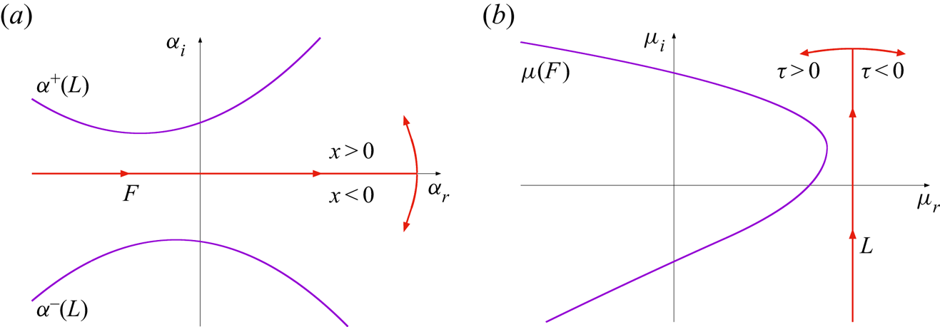
The approach for characterising unstable disturbances is equivalent to that presented by Brevdo & Bridges (Reference Brevdo and Bridges1997) with the exception of the rotation in the complex frequency plane that arises as a consequence of the differing representations of the temporal component of the perturbation. Equation (4.7) is evaluated for contours  $F$ and
 $L$ in the respective complex
 $\alpha$- and
 $\mu$-planes, which are indicated by the respective horizontal and vertical red lines in figure 2. Closure of the two contours,
 $F$ and
 $L$, is then achieved by adding a contour that connects the respective endpoints. Since the integrand is zero along this closure, the integral solution (4.7) along the straight-line open contour is equivalent to that obtained over the closed contour. Thus, by Cauchy's residue theorem, the integral is the sum of the residues of the poles contained within the closed contour.
Sketches illustrating the initial set-up for Briggs’ method. (a) Complex  $\alpha$-plane. (b) Complex
 $\mu$-plane.

In the complex  $\alpha$-plane, depicted in figure 2(a), the integrand in (4.7) decays as
 $\alpha _i \rightarrow \infty$ for
 $x>0$. Thus, the horizontal
 $F$ contour can be closed by a semi-circular contour of infinite radius in the upper half-plane. Hence, when
 $x>0$, the integral along
 $F$ is determined by summing the residues of poles in the upper half-plane. Similarly, if
 $x < 0$, closure is achieved by a semi-circular contour in the lower half-plane and the integral along
 $F$ is given by summing the residues of poles in the lower half-plane.
For each  $\alpha \in F$ there are
 $\mu$-roots to the dispersion relation
 $D(\alpha ,\mu ) = 0$ that correspond to poles of the integrand in (4.7). Taking the loci of these poles for all
 $\alpha \in F$ establishes
 $\mu (F)$ curves in the complex
 $\mu$-plane. The
 $\mu (F)$ curve located furthest to the right in the complex
 $\mu$-plane is illustrated by the solid purple curve in figure 2(b). The vertical
 $L$ contour is then chosen to lie to the right of this curve by selecting the real part as
 \begin{equation} \sigma > max \left\{\mu_r \,|\, D(\alpha,\mu) = 0,\ \forall\ \alpha \in \mathbb{R} \right\}. \end{equation}
Similar to the approach implemented for the  $F$ contour, closure of the
 $L$ contour in the complex
 $\mu$-plane is achieved via the addition of semi-circular contours to the left or right. The integrand in (4.7) decays as
 $\mu _r \rightarrow \infty$ for time
 $\tau < 0$. Thus, provided there are no poles to the right of the
 $L$ contour, the integral must be zero. Hence, the disturbance is zero for all points in time prior to the application of the impulsive forcing
 $\boldsymbol {g}$. Therefore, it is necessary that
 $\sigma$ is given by (4.8) to satisfy causality. For time
 $\tau > 0$, closure is achieved by a semi-circular contour to the left of the
 $L$ contour. This closed contour then contains all poles of the integrand in (4.7).
For Floquet exponents  $\mu \in L$,
 $\alpha ^{\pm }(L)$ curves in the complex
 $\alpha$-plane satisfy the dispersion relation
 $D(\alpha ,\mu ) = 0$ and describe poles of the integrand in (4.7), as depicted by the solid purple curves in figure 2(a). Initially, all poles are associated with spatial decay, while
 $\alpha ^{\pm }(L)$ represent those curves that exhibit the slowest decay along the positive and negative valued
 $x$-directions.
The Fourier integral (4.5) in (4.7) is computed first, which is given as
 \begin{equation} \boldsymbol{\psi}(x^{{\pm}},\mu) = \frac{1}{2{\rm \pi}} \oint_{C_F^{{\pm}}} {\boldsymbol{\mathsf{Q}}}\left(\alpha,\tau\right) \frac{{\boldsymbol{\mathsf{G}}}\left(\alpha,\mu\right)}{D\left(\alpha,\mu\right)} \exp(\textrm{i} \alpha x^{{\pm}}) \,\mathrm{d} \alpha, \end{equation}
for some  $\mu$, where
 $x^+$ and
 $x^-$ are shorthand for
 $x > 0$ and
 $x < 0$, respectively. Similarly,
 $C_F^{\pm }$ denotes the closed contour for a particular
 $x$ value. Due to the adoption of this compact notation, two expressions are represented by (4.9). A single expression for all
 $x$ is given by
 \begin{equation} \boldsymbol{\psi}(x,\mu) = H(x) \boldsymbol{\psi}(x^+,\mu) + H({-}x) \boldsymbol{\psi}(x^-,\mu), \end{equation}
where  $H(x)$ is the Heaviside function. Furthermore, by Cauchy's residue theorem
 \begin{equation} \boldsymbol{\psi}(x^{{\pm}},\mu) ={\pm} \textrm{i} \sum_{k = 1}^{\infty} {\boldsymbol{\mathsf{Q}}}\left(\alpha_k^{{\pm}}\left(\mu\right),\tau\right) \frac{ {\boldsymbol{\mathsf{G}}} \left( \alpha_k^{{\pm}}\left(\mu\right), \mu \right)}{\dfrac{\partial D}{\partial \alpha} \left( \alpha_k^{{\pm}}\left(\mu\right),\mu \right)} \exp(\textrm{i} \alpha_k^{{\pm}}\left(\mu\right) x^{{\pm}}), \end{equation}
where  $\alpha ^+_k(\mu )$ and
 $\alpha ^-_k(\mu )$ are the roots of the dispersion relation
 $D(\alpha ,\mu ) = 0$ in the upper and lower halves of the complex
 $\alpha$-plane, respectively.
On solving the Fourier integral (4.9), the Laplace integration (4.6) is carried out. This is achieved by deforming the  $L$ contour to the left in the complex
 $\mu$-plane. To illustrate this behaviour, we consider one particular
 $\mu$ value on
 $L$ with a fixed imaginary part
 $\mu _i$. The corresponding real part,
 $\mu _r$, is then reduced. The problem then simplifies to tracing the behaviour of poles in the complex
 $\alpha$-plane as the real part of
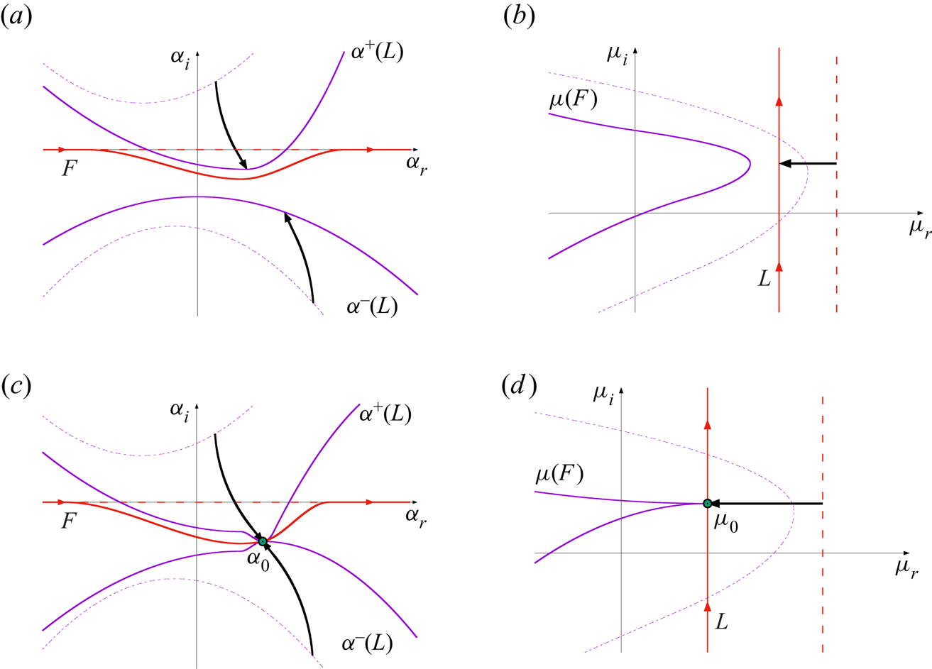
 $\mu$ is shifted horizontally to the left. Figure 3 demonstrates both the behaviour about a fixed
 $\mu _i$ value and the overall deformation of the contours and curves when all
 $\mu _i$ are considered. The leftwards shift of a fixed
 $\mu$ value and the corresponding movement of the
 $\alpha$-roots are illustrated by arrows in the respective
 $\mu$- and
 $\alpha$-planes; figure 3(a,b). The deformation of the
 $L$ contour in the
 $\mu$-plane and that of the corresponding
 $F$ contour in the
 $\alpha$-plane are made more obvious by the inclusion of the initial set-up (represented by dashed purple and red lines).
Sketches illustrating the pinching of the  $F$ contour in the complex
 $\alpha$-plane as the contour
 $L$ is shifted horizontally to the left in the complex
 $\mu$-plane. Arrows indicate the behaviour brought about by the horizontal movement of a fixed Floquet exponent
 $\mu$, dashed lines indicate the original contours and pole loci (as per figure 2), while solid curves demonstrate the deformations due to the leftward movement of the
 $L$ contour; (a,b)
 $\mu$ is reduced until one
 $\alpha$-root crosses the real
 $\alpha$-axis, (c,d)
 $\mu =\mu _0$ corresponds to a collision of poles at
 $\alpha _0$.

As the real part of the Floquet exponent is reduced, the resulting path will eventually cross the  $\mu (F)$ curve, which describes the
 $\mu$-roots of the dispersion relation
 $D(\alpha ,\mu ) = 0$ for
 $\alpha \in \mathbb {R}$; dashed purple curve in figure 3(b). Thus, at least one
 $\alpha$-root of
 $D$ lies along the real
 $\alpha$-axis. Moving
 $\mu$ beyond the
 $\mu (F)$ curve allows one
 $\alpha$-root to cross over the
 $F$ contour and pass from one half of the complex
 $\alpha$-plane to the other; as demonstrated by the arrow originating in the upper right quadrant in figure 3(a). Since a pole has shifted from one half of the complex
 $\alpha$-plane to the other, there is a discontinuity in (4.11) for
 $\boldsymbol {\psi }$, with the jump being the size of the residue of this particular pole. However, an analytic continuation of
 $\boldsymbol {\psi }$ is achieved by deforming the
 $F$ contour, as shown in figure 3(a), to ensure that all
 $\alpha$-roots remain on their respective sides of
 $F$. The modification of the
 $F$ contour results in a corresponding deformation of the
 $\mu (F)$ curve in figure 3(b).
By allowing for the deformation of the  $F$ contour, the horizontal shifting of the Floquet exponent
 $\mu$ can be extended to smaller valued
 $\mu _r$. However, in general, this procedure cannot be continued indefinitely. Once an
 $\alpha$-root has crossed into the opposite half-plane, the leftwards shift to some
 $\mu = \mu _0$ is accompanied by the coalescence at
 $\alpha _0$ of two poles originating in different halves of the complex
 $\alpha$-plane, as demonstrated in figure 3(c,d). The
 $F$ contour becomes pinched and passes through the pole at
 $\alpha _0$, but cannot be deformed further without introducing discontinuities in
 $\boldsymbol {\psi }$. Thus, a further reduction in
 $\mu _r$ is not possible. Note that a coalescence of
 $\alpha$-roots originating within the same half-plane does not pinch the
 $F$ contour.
The coalescence of two simple poles at  $\alpha _0$ results in a second-order pole. Therefore, in addition to satisfying the dispersion relation
 \begin{equation} D(\alpha_0,\mu_0) = 0, \end{equation}
it must also hold that
 \begin{equation} \frac{\partial D}{\partial \alpha} (\alpha_0,\mu_0) = 0. \end{equation}
Thus, such collisions manifest as saddle points of the dispersion relation in the complex  $\alpha$-plane. Moreover, by inverting this relationship it becomes evident that the formation of a saddle point at
 $\alpha _0$ is accompanied by the formation of a cusp at
 $\mu _0$ (Kupfer, Bers & Ram Reference Kupfer, Bers and Ram1987), as illustrated by the solid purple curve in figure 3(d).
In (3.3), which is equivalent to the dispersion relation  $D(\alpha ,\mu ) = 0$, the wavenumber
 $\alpha$ appears to the fourth order, while the Floquet exponent
 $\mu$ is linear. Since the matrices in the eigenvalue problem (3.10) are very large, it was computationally impossible to determine
 $\alpha$ for a given
 $\mu$ using the currently available computational resources. Hence, it was not feasible to locate saddle points of the dispersion relation in the complex
 $\alpha$-plane. Nevertheless, utilising existing methods for computing
 $\mu$ for a given
 $\alpha$, the corresponding cusps of the dispersion relation in the complex
 $\mu$-plane may be located.
Using a Taylor series expansion for  $\boldsymbol {\psi }$ about
 $\alpha _0$, it may be shown that if
 $\alpha _0$ is formed by the collision of two poles originating in the opposite halves of the
 $\alpha$-plane, then it contributes to the expressions (4.9)–(4.11) for both positive and negative valued
 $x$. Hence, the parameter set
 $(\alpha _0,\mu _0)$ contributes to the pointwise asymptotic behaviour of the disturbance. A similar argument can be used to demonstrate that if
 $\alpha _0$ represents the collision of two poles originating in the same half-plane, there is a cancellation effect and the collision does not contribute to the asymptotic behaviour (Huerre Reference Huerre2002). The condition that the collision occurs between poles originating in opposite half-planes is known as the collision criterion (Brevdo & Bridges Reference Brevdo and Bridges1997).
Finally, the Laplace integration in (4.7) is carried out along a contour that lies to the right of every  $\mu _0$; there can be multiple such branch points, potentially a continuum, due to the continuous choice of
 $\mu _i$ at the start of the procedure. For a collision that satisfies the collision criterion, the leading-order behaviour is then described by
 \begin{equation} \boldsymbol{\psi}(x,\tau) \sim \frac{- \textrm{i}{\boldsymbol{\mathsf{Q}}}(\alpha_0,\tau) {\boldsymbol{\mathsf{G}}}\left(\alpha_0,\mu_0\right)}{\sqrt{ 2 {\rm \pi}\tau \dfrac{\partial D}{\partial \mu} \left( \alpha_0, \mu_0 \right) \dfrac{\partial^2 D}{\partial \alpha^2} \left( \alpha_0, \mu_0 \right) }} \exp\left(\textrm{i} \alpha_0 x + \mu_0 \tau\right), \end{equation}
where  $\alpha _0$ is the location of the pinch-type saddle point in the complex
 $\alpha$-plane and
 $\mu _0$ is the corresponding cusp location. While there are notionally multiple such values, the leading-order behaviour of (4.13) is described by the pair
 $(\alpha _0,\mu _0)$ for which
 $\mu _0$ has the greatest real part. It is possible to account for lower-order behaviour by considering a superposition of similar expressions for further
 $(\alpha _0,\mu _0)$ pairs.
The expression for the streamfunction  $\boldsymbol {\psi }$, as given in (4.13), matches the Floquet mode decomposition given in (3.2), up to a multiplication by a factor
 $1/\sqrt {\tau }$. Pointwise temporal growth occurs if
 $\mbox {Re}\{\mu _0\} > 0$, while
 $\mbox {Re}\{\mu _0\} < 0$ corresponds to pointwise decay. In the former instance, the disturbance is classified as absolutely unstable, while in the latter case the disturbance is either convectively unstable or stable (depending on the growth or decay of the disturbance maximum).
4.3. Symmetry constraints
In addition to being periodic with a period  $2{\rm \pi}$, the temporal variation of the basic state (2.2) is antiperiodic with an antiperiod
 ${\rm \pi}$; i.e.
 $U_B(y,\tau +{\rm \pi} ) = -U_B(y,\tau )$. Thus, the distinction between the upstream and downstream
 $x$-directions is blurred, and the location of the roots of the dispersion relation
 $D(\alpha _0,\mu _0) = 0$ are constrained. This behaviour is illustrated by considering the governing perturbation equation (3.3), that is equivalent to the dispersion relation, whereby the solution is characterised by the complex-valued wavenumber
 $\alpha$, Floquet exponent
 $\mu$, and eigenfunction
 $\psi$:
 \begin{equation} \left(\alpha,\mu,\psi\left(y,\tau\right)\right). \end{equation}
On taking the complex conjugate of (3.3), the governing perturbation equation remains unchanged but the solution is now characterised as
 \begin{equation} \left(-\bar{\alpha},\bar{\mu},\bar{\psi}\left(y,\tau\right)\right), \end{equation}
where  $\bar {z}$ denotes the complex conjugate of
 $z$. The existence of the solution (4.14a) implies the existence of the solution (4.14b), and this relationship holds irrespective of the antiperiodicity of the flow. Returning to (3.3) and applying a time shift of half a period,
 $\tau \rightarrow \tau + {\rm \pi}$, the sign of the basic state is reversed and the asymptotic behaviour for large time
 $\tau$ is unchanged. Thus, the solution is given as
 \begin{equation} \left(-\alpha,\mu,\psi\left(y,\tau+{\rm \pi}\right)\right). \end{equation}
The existence of the solution (4.14a) implies the existence of the solution (4.14c) when antiperiodicity holds. Applying both complex conjugation and a time shift of half a period to (3.3), the solution is characterised as
 \begin{equation} \left(\bar{\alpha},\bar{\mu},\bar{\psi}\left(y,\tau+{\rm \pi}\right)\right). \end{equation}
It follows from the related solutions (4.14) that for any given pair  $(\alpha ,\mu )$ that satisfy (3.3),
 \begin{equation} D(\alpha,\mu) = 0 \Longrightarrow \left\{\begin{matrix} D(\bar{\alpha},\bar{\mu}) = 0, \\ D(-\alpha,\mu) = 0, \\ D(-\bar{\alpha},\bar{\mu}) = 0, \end{matrix}\right. \end{equation}
for any antiperiodic flow.
In the instance  $\alpha \in \mathbb {R}$, such that
 $\bar {\alpha } = \alpha$, the set of relationships (4.15) reduce to
 \begin{equation} D(\alpha,\mu) = 0 \Longrightarrow \left\{\begin{matrix} D(\alpha,\bar{\mu}) = 0, \\ D(-\alpha,\mu) = 0, \\ D(-\alpha,\bar{\mu}) = 0. \end{matrix}\right. \end{equation}
Hence, for any  $\alpha \in \mathbb {R}$, the
 $\mu$-roots of the dispersion relation
 $D(\alpha _0,\mu _0) = 0$, appear in complex conjugate pairs. In terms of Briggs’ method, this implies that the
 $\mu (F)$ curve, plotted in figure 2(b), is symmetric about the real
 $\mu$-axis.
A similar argument can be established for Floquet exponents  $\mu$, once the harmonic decomposition of
 $\mu$ in (3.5) has been taken into account. The imaginary part of the Floquet exponent,
 $\mu _i$, is only given modulo one, since an integer shift is equivalent to a relabelling of the harmonics. Thus,
 \begin{equation} D(\alpha,\mu) = 0 \Longrightarrow D(\alpha,\mu+ik) = 0, \end{equation}
for all integers  $k$. Moreover, in the instance that
 $\mu _i$ is a multiple of
 $1/2$, complex conjugation is equivalent to an integer shift in
 $\mu _i$. Therefore,
 \begin{equation} D(\alpha,\mu) = 0 \Longrightarrow D(\alpha,\bar{\mu}) = 0, \end{equation}
where, restricting our interest to the interval  $\mu _i \in [ 0,1 )$ gives
 \begin{equation} \mu = \mu_r + \textrm{i} \left\{0,\tfrac{1}{2} \right\} \quad \textrm{for}\ \mu_r \in \mathbb{R}. \end{equation}
On applying the above symmetries, it follows that, for all  $\mu$ of the form (4.19), the set of relationships (4.15) reduces to
 \begin{equation} D(\alpha,\mu) = 0 \Longrightarrow \left\{\begin{matrix} D(\bar{\alpha},\mu) = 0, \\ D(-\alpha,\mu) = 0, \\ D(-\bar{\alpha},\mu) = 0. \end{matrix}\right. \end{equation}
In the pinch-point analysis described above, the imaginary part of  $\mu$ is fixed and the
 $\alpha$-roots of the dispersion relation
 $D(\alpha ,\mu ) = 0$ are traced as the real part of
 $\mu$ is shifted horizontally to the left (recall § 4.2). When the imaginary part of
 $\mu$ is fixed such that
 $\mu _i=\{0,1/2\}$, the movement of the
 $\alpha$-roots is constrained by the symmetries of the base flow (2.2) and hence (4.20) holds. In particular, if the wavenumber
 $\alpha$ is a root of the dispersion relation
 $D(\alpha ,\mu ) = 0$, then so are the wavenumbers
 $\bar {\alpha }$,
 $-\alpha$ and
 $-\bar {\alpha }$. Thus, once
 $\mu$ comes into contact with the
 $\mu (F)$ curve and an
 $\alpha$-root touches the real axis, the corresponding
 $\bar {\alpha }$-root must also touch the real axis. Similarly for
 $-\alpha$ and
 $-\bar {\alpha }$. Hence, the
 $F$ contour is pinched along the real
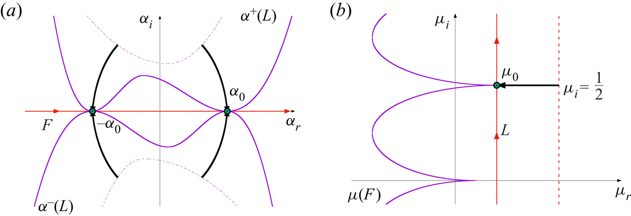
 $\alpha$-axis and no contour deformation is necessary. This behaviour is demonstrated in figure 4 for
 $\mu _i = 1/2$. Since the
 $F$ contour is not deformed, neither is the
 $\mu (F)$ curve, though the existence of the saddle point at
 $\alpha _0 \in \mathbb {R}$ (and
 $-\alpha _0$) indicates a cusp at
 $\mu _0$, as illustrated in figure 4(b). Moreover, there is a cusp indicated for
 $\mu _i = 0$, by the same argument. Note that the
 $\alpha ^{\pm }(L)$ curves are not symmetric, even though the movement of the
 $\alpha$-roots associated with
 $\mu _i = \{0,1/2\}$ are symmetric along both axes.
Sketches illustrating the pinching of the  $F$ contour along the real
 $\alpha$-axis, when
 $\mu = \mu _r + i/2$. (a) Complex
 $\alpha$-plane. (b) Complex
 $\mu$-plane. For the horizontal line extending from the
 $L$ contour to the
 $\mu (F)$ curve, there is a matching symmetric movement of the
 $\alpha$-roots that form collisions along the real
 $\alpha$-axis about
 $\pm \alpha _0$.

The existence of these pinch points is assured by the process outlined in § 4.2, when the  $\mu (F)$ curve is well defined for
 $\mu _i = \{0,1/2\}$. The
 $L$ contour in figure 2(b) contains all possible values of
 $\mu _i$, including
 $0$ and
 $1/2$, while the
 $\mu (F)$ curve (corresponding to
 $\alpha \in \mathbb {R}$) must lie to the left of the
 $L$ contour to satisfy causality. Furthermore, as
 $\mu$ is shifted to the left for
 $\mu _i = \{0,1/2\}$, the
 $\mu (F)$ curve is eventually reached. Hence, by the symmetry arguments described above, a collision of complex conjugate
 $\alpha$-roots occurs. There is a possibility that in some antiperiodic flows the
 $\mu (F)$ curve is not well defined for
 $\mu _i = \{0,1/2\}$, i.e. there are no real
 $\alpha$ corresponding to these particular
 $\mu _i$ values. However, this was not the case for the Stokes layer studied herein and so is not discussed any further, but is highlighted as a potential factor in other antiperiodic flows.
The above analysis indicates that saddle points of the dispersion relation  $D(\alpha ,\mu ) = 0$, satisfying the collision criteria, occur whenever
 $\alpha \in \mathbb {R}$ and
 $\mu _i = \{0,1/2\}$; collisions emerge between complex conjugate
 $\alpha$-roots. Moreover, for these particular
 $\mu _i$ values, the collision of two
 $\alpha$-roots originating within the same half-plane onto the real axis will be accompanied by the collision of their respective complex conjugates in a four-way collision. Thus, all saddle points of the dispersion relation with these characteristics must satisfy the collision criteria.
Further collisions may occur for  $\mu _i\neq \{0,0.5\}$ (as
 $\mu$ crosses the
 $\mu (F)$ curve) that bring about greater pointwise growth than that found for
 $\mu _i = \{0,1/2\}$. In such instances, this may necessitate a deformation of the
 $F$ contour and establish a pinch point with the
 $\mbox {Re}\{\mu _0\}$ greater than that found using the symmetry arguments. However, while such behaviour may be significant for other flows, this was not found for the Stokes layer: the rightmost point of the
 $\mu (F)$ curve was matched to a cusp with
 $\alpha \in \mathbb {R}$ and
 $\mu _i = 0$ in every case considered.
4.4. Development of the disturbance maximum
In addition to determining the disturbance development about fixed spatial locations (via the Briggs method), the integral solution (4.7) provides insight into the leading-order behaviour of the disturbance maximum. The stability of a disturbance  $\boldsymbol {\psi }$ to an impulse
 $\boldsymbol {g}$ can be determined by generalising the problem to consider the leading-order behaviour along an arbitrary spatio-temporal ray
 \begin{equation} x/\tau = V, \end{equation}
where  $V$ is constant.
In this setting, the leading-order pointwise behaviour (deduced by the Briggs method) corresponds to  $V=0$. On the other hand, the temporal growth associated with the disturbance maximum is matched to the spatio-temporal ray
 $V = V_{max}$. The growth rate along this particular ray is of interest as Ramage et al. (Reference Ramage, Davies, Thomas and Togneri2020) report that the temporal growth about fixed spatial locations matches that of the disturbance maximum.
Similar to the arguments used for steady flows, the Floquet mode (3.2) that contributes towards the growth (or decay) of the disturbance along the ray  $V_{max}$ corresponds to
 $\alpha \in \mathbb {R}$ and
 \begin{equation} \frac{\partial \mu_r}{\partial \alpha} = 0. \end{equation}
This particular result is derived by solving the integral equation (4.7) along a spatio-temporal ray by the method of steepest descent (refer to Ramage (Reference Ramage2017), for details). It follows that the asymptotic temporal growth of the disturbance maximum can be determined by plotting the real part of the Floquet exponent  $\mu$ as a function of the real wavenumber
 $\alpha$, and selecting the maximum.
For antiperiodic flows, such as (2.2), the asymptotic temporal growth of the disturbance maximum and the asymptotic pointwise growth correspond to  $\alpha \in \mathbb {R}$. Hence, the growth rate along the ray
 $V_{max}$ and the pointwise growth rate along
 $V = 0$ can be equivalent, provided the collision location along the real
 $\alpha$-axis corresponds to a local maximum of
 $\mu _r$.
5. Results
The impulse response of linear disturbances in the Stokes layer was first investigated by Thomas et al. (Reference Thomas, Davies, Bassom and Blennerhassett2014) and then subsequently by Ramage et al. (Reference Ramage, Davies, Thomas and Togneri2020) via DNS. It was revealed that the family-tree structure develops (as depicted in figure 1), which consists of a mother wavepacket giving birth to two daughter wavepackets during each period of wall motion. One wavepacket propagates to the left, while the second convects to the right. These two daughter wavepackets birth granddaughter wavepackets and so on, giving rise to the so-called family-tree formation. It was observed that the disturbance maximum propagates along successive wavepackets in the direction dictated by the phase of the wall motion at the time at which the impulsive forcing was applied (to the right in figure 1). Additionally, the spatial distance between adjacent wavepackets is fixed by the Reynolds number  ${Re}$, and so granddaughter wavepackets manifest in the same streamwise
 $x$-location as the mother wavepacket, resulting in an increase in the disturbance magnitude every two periods of wall motion. Thus, subharmonic growth occurs about fixed spatial positions, i.e. pointwise growth with a periodicity twice that of the basic state. Furthermore, the temporal growth about fixed spatial locations was found to match the growth of the disturbance maximum. Hence, DNS results suggest that the Stokes layer is subject to an absolute form of instability. However, such behaviour can only be confirmed theoretically via the application of the Briggs criteria.
Harmonic and subharmonic behaviour can be associated with the imaginary part of the Floquet exponent  $\mu$ in (4.19) that was highlighted as being significant in the symmetry arguments described above; recall
 $\mu _i = \{0,1/2\}$. In the instance
 $\mu _i = 0$, a stationary Floquet mode of the form (3.2) has the same periodicity as the basic state (2.2), with behaviour described as harmonic. On the other hand, when
 $\mu _i = 1/2$, the imaginary part of the Floquet exponent can be absorbed into the periodic streamfunction
 $\psi$ in (3.2), resulting in a period twice that of the basic state. This behaviour is subharmonic and describes the pointwise behaviour observed in the earlier DNS computations. These two particular cases are distinct from the more general Floquet mode form, in which the disturbance amplification is accompanied by a phase shift.
5.1. Floquet analysis
5.1.1. Eigenspectra
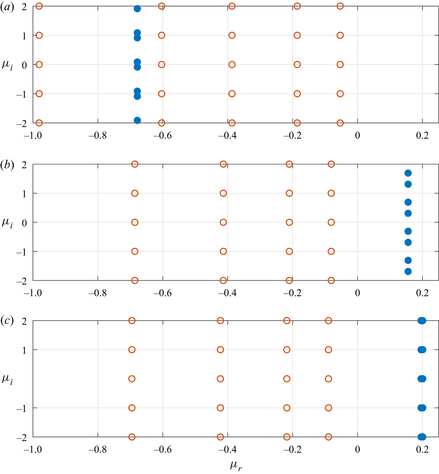
Before we undertake an investigation of absolute instability in the Stokes layer, a linear stability analysis is performed to validate the numerical scheme and to report on the complex stability characteristics first presented by Blennerhassett & Bassom (Reference Blennerhassett and Bassom2002, Reference Blennerhassett and Bassom2006). Figure 5 displays a subset of the eigenvalues of (3.10) in the complex  $\mu$-plane, for the Reynolds number
 ${Re}=750$ and wavenumbers
 $\alpha =0.25$,
 $0.35$ and
 $0.3747$. Open red circular markers represent centre modes that were first reported in Von Kerczek & Davis (Reference Von Kerczek and Davis1974) and subsequently by Blennerhassett & Bassom (Reference Blennerhassett and Bassom2006) for oscillatory flow in a channel. Multiple decaying centre modes
 $\gamma$ (with a negative real component and a zero imaginary component) are found along the real
 $\mu$-axis and then at
 $\mu =\gamma +\textrm {i}k$ for all integers
 $k$. These particular perturbations are associated with disturbance development in the channel centre and are always linearly stable for the range of Reynolds numbers modelled in this study. Solid blue circular markers correspond to the Stokes mode that is of primary interest here. For each Floquet exponent
 $\mu$ there is a corresponding complex conjugate
 $\bar {\mu }$. This complex conjugate pair are then matched to left- and right-travelling waves with equal growth. Additionally, there are equivalent Floquet exponents
 $\mu +\textrm {i}k$ for all integers
 $k$. Hence, the imaginary part of the Floquet exponent can be restricted to the interval
 $\mu _i\in [0,0.5]$ for the remainder of this study.
Floquet exponents  $\mu$ in the complex
 $\mu$-plane for the Reynolds number
 ${Re}=750$ and wavenumbers (a)
 $\alpha =0.25$, (b)
 $\alpha =0.35$ and (c)
 $\alpha =0.3747$. Solid blue circles are matched to the Stokes mode, while open red circles are matched to centre modes.

For the wavenumber  $\alpha =0.25$, the Floquet exponent
 $\mu$ has a negative real part, i.e.
 $\mu _r<0$. Thus, the disturbance is linearly stable for this particular wavenumber. However, as
 $\alpha$ increases to
 $0.35$ and
 $0.3747$, the Floquet exponent crosses the
 $\mu _r=0$ axis and becomes positive, leading to linearly unstable behaviour. Interestingly, for
 $\alpha =0.3747$, the left- and right-travelling waves (given by the complex conjugate pair
 $\mu$ and
 $\bar {\mu }$) coalesce to form two stationary waves but with marginally different growth rates. This particular phenomenon was first discovered by Blennerhassett & Bassom (Reference Blennerhassett and Bassom2002) and leads to the formation of finger-like structures along the neutral stability curve.
5.1.2. Neutral stability curve
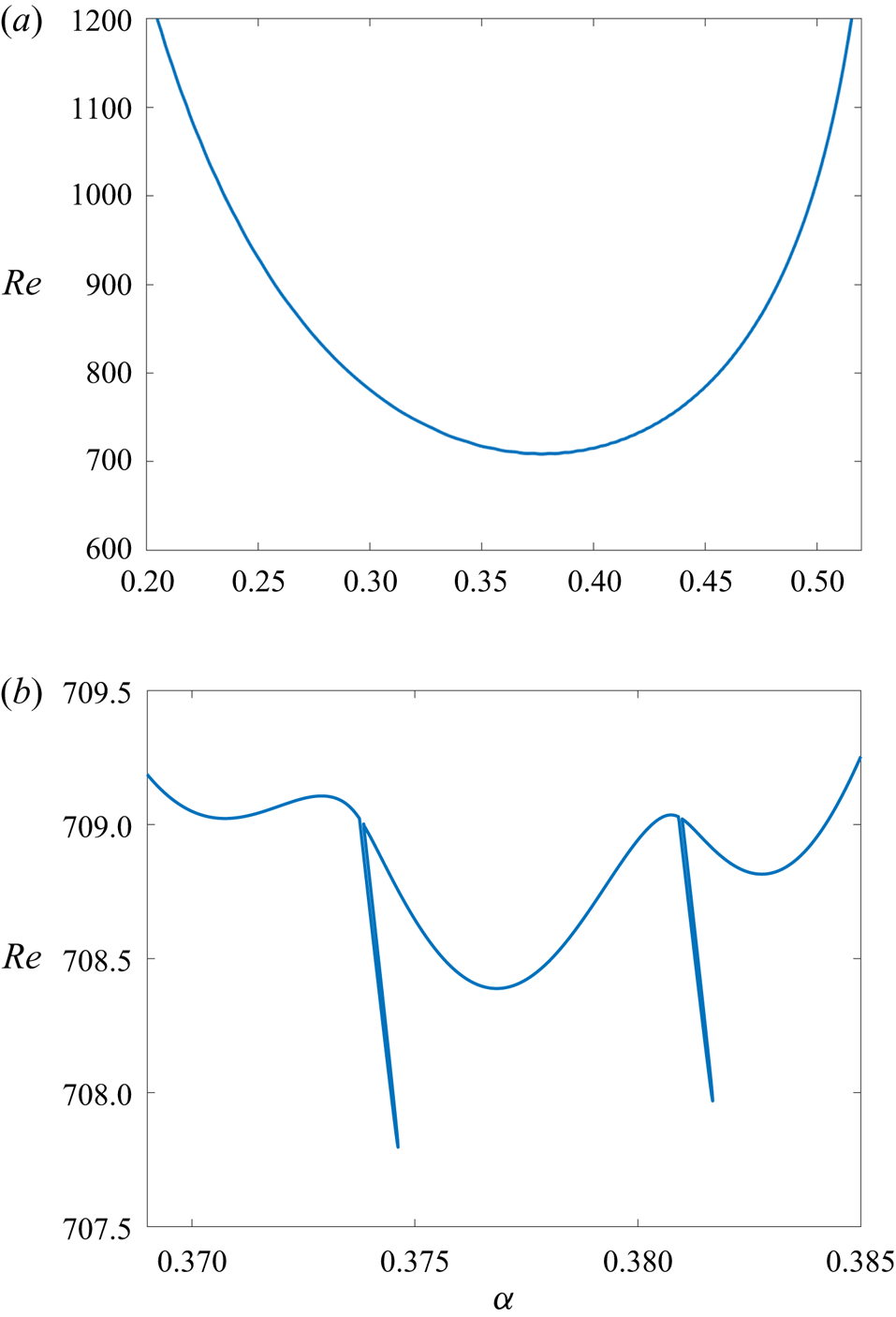
Neutral points  $(\alpha ,{Re})$ for linear instability were determined (i.e.
 $\mu _r=0$), with sections of the neutral stability curve plotted in figure 6. In figure 6(a), the neutral curve is plotted over a large
 $\alpha$-domain and appears smooth. Here (and for the remainder of this study) the analysis has been restricted to wavenumbers
 $\alpha \leq 0.52$, as following Blennerhassett & Bassom (Reference Blennerhassett and Bassom2002), linearly unstable behaviour is not expected for larger valued
 $\alpha$. The critical Reynolds number
 ${Re}_c$ corresponds to the lowest point along this curve, below which all disturbances are linearly stable. In figure 6(b), the neutral curve is plotted over a reduced
 $\alpha$-range, localised about the critical conditions for linear instability. The critical Reynolds number
 ${Re}_c = 707.84$ is located about the tip of one of the finger-like protrusions that extend vertically downwards from the main body of the neutral stability curve. As reported in Blennerhassett & Bassom (Reference Blennerhassett and Bassom2002), these finger-like features occur at regular wavenumber intervals and are matched to stationary disturbances, i.e.
 $\mu _i=0$.
Neutral curve for linear instability in the  $(\alpha ,{Re})$-plane. (a) Large
 $\alpha$-domain. (b) Reduced
 $\alpha$-domain about the critical conditions for instability.

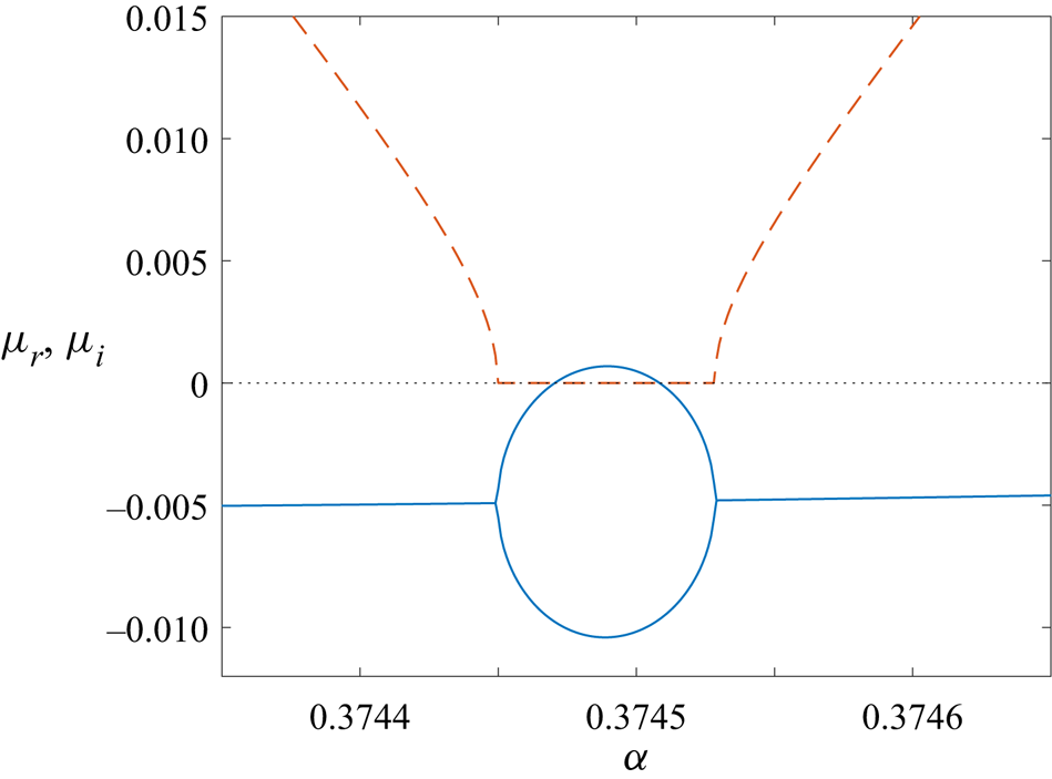
Figure 7 depicts the variation of the real (solid line) and imaginary (dashed line) parts of the Floquet mode  $\mu$ as a function of the wavenumber
 $\alpha$, for the Reynolds number
 ${Re}=708$. Results are plotted about the region where linearly unstable stationary modes develop and corresponds to a horizontal cut through the leftmost finger in figure 6(b). There is a small wavenumber interval about
 $0.37445<\alpha <0.37455$ that
 $\mu _i$ is zero, leading to the emergence of stationary waves. Outside of this interval,
 $\mu _i$ is non-zero. (Note that for consistency with the presentation of figure 1 of Blennerhassett & Bassom (Reference Blennerhassett and Bassom2002), when the Floquet exponent
 $\mu$ is complex, only eigenvalues corresponding to
 $\mu _i>0$ are plotted in figure 7; the complex conjugate
 $\bar {\mu }$ has been omitted.) At the left end point of this interval, stable left- and right-travelling waves (corresponding to
 $\mu$ and
 $\bar {\mu }$) coalesce to form two stationary waves. Significantly, the two stationary waves have very different growth rates over this interval, with one becoming marginally unstable. This behaviour is consistent with the formation of the leftmost finger-like protrusion in figure 6(b). As the wavenumber
 $\alpha$ increases, the two stationary waves re-establish the two stable travelling waves with equal growth
 $\mu _r$ but opposite sign
 $\mu _i$. This particular stability feature of the Stokes layer is not restricted to Floquet modes along the neutral stability curve, but is found throughout the
 $(\alpha ,{Re})$ parameter space.
Variation of the real and imaginary parts of the Floquet exponent  $\mu$ as a function of the wavenumber
 $\alpha$ in a region that
 $\mu _i=0$. Here the Reynolds number
 ${Re}=708$; solid and dashed lines depict the real
 $\mu _r$ and imaginary
 $\mu _i$ components.

5.1.3. Temporal growth of the disturbance maximum
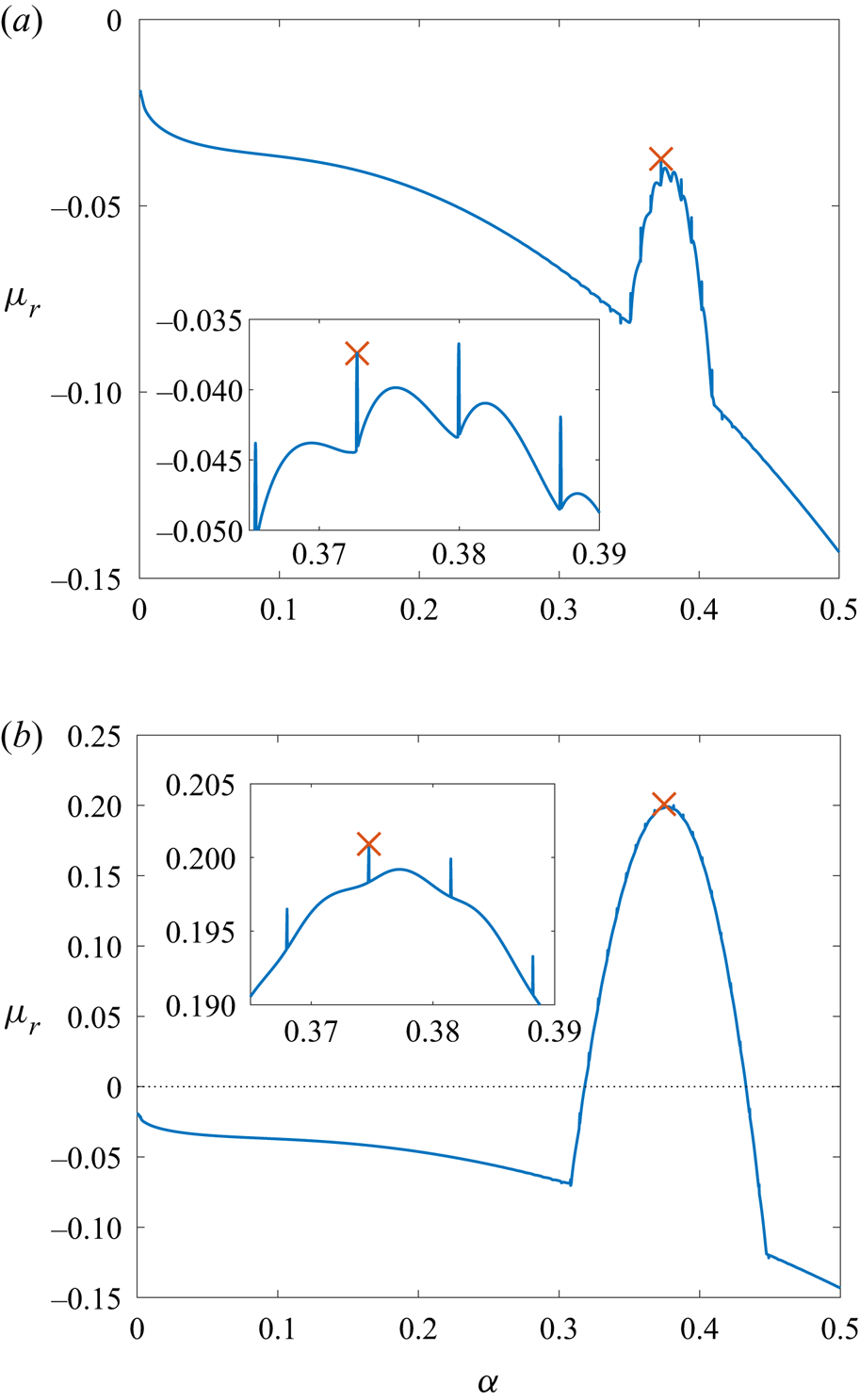
Floquet calculations for the growth rate  $\mu _r$ are compared against the DNS computations of Ramage et al. (Reference Ramage, Davies, Thomas and Togneri2020), who numerically determined the growth rate of the disturbance maximum. Figure 8 depicts the variation of the Floquet growth rate
 $\mu _r$, for Reynolds numbers
 ${Re} = 700$ and
 ${Re} = 750$, over the wavenumber interval
 $\alpha \in [0,0.5]$. The local maximum that satisfies condition (4.22) is indicated by a red cross marker. Within each subplot, magnified insets highlight those modes with the largest growth rate
 $\mu _r$. In both instances, the local maximum is located about the tip of a finger-like protrusion and are comparable to those structures found along the neutral stability curve in figure 6 that are brought about by the appearance of stationary waves. In figure 8(a), larger (less negative) growth rates are observed for wavenumbers
 $\alpha$ near zero but correspond to the centre modes
 $\gamma$ and have been disregarded as they do not satisfy the local maximum condition (4.22).
Floquet growth rate  $\mu _r$ as a function of the real wavenumber
 $\alpha$ for (a)
 ${Re} = 700$ and (b)
 ${Re} = 750$. The largest growth rate that satisfies (4.22) is indicated by red cross markers;
 $(\alpha ,\mu _r) = (0.3727,-0.0374)$ for
 ${Re}=700$ and
 $(\alpha ,\mu _r) = (0.3747,0.2009)$ for
 ${Re}=750$.

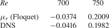
Table 1 compares those Floquet growth rates  $\mu _r$ that achieve a maximum in figure 8 against the equivalent DNS computations obtained by Ramage et al. (Reference Ramage, Davies, Thomas and Togneri2020). Growth rates agree to two decimal places, which is excellent given that the DNS calculations were based on measurements taken after a finite time interval. Thus, small differences are to be expected.
Floquet growth rate  $\mu _r$ for the least-stable mode with
 $\alpha \in \mathbb {R}$ (see figure 8), compared against the DNS computations of Ramage et al. (Reference Ramage, Davies, Thomas and Togneri2020).

In both illustrations shown in figure 8, maximum growth rates are located at the tip of finger-like protrusions. Since these protruding features correspond to stationary waves with both  $\mu _i = 0$ and
 $\alpha _i = 0$, which was highlighted in § 4.3 as implying the location of pinch points in antiperiodic flows, this is an appropriate starting point for the search of absolutely unstable behaviour.
5.2. Absolute instability
5.2.1. Approach I: $\alpha \in \mathbb {C}$

As discussed in § 4, those modes that contribute to the asymptotic pointwise growth of the impulse response and classify the disturbance as convectively or absolutely unstable can be determined by locating cusps of the dispersion relation  $D(\alpha ,\mu ) = 0$ in the complex
 $\mu$-plane. This is achieved by numerically solving the eigenvalue problem (3.3) and mapping solutions from the complex
 $\alpha$-plane onto the complex
 $\mu$-plane. Given the symmetry arguments outlined above for antiperiodic flows, cusps matched to
 $\alpha _i = 0$ and
 $\mu _i = \{0,1/2\}$ satisfy the collision criteria and hence establish absolute instability.
The emergence of cusps in the complex  $\mu$-plane and absolutely unstable behaviour will be demonstrated first (and in the most detail) for the Reynolds number
 ${Re} = 750$, which corresponds to a strongly unstable disturbance, as illustrated by the positive Floquet growth rate
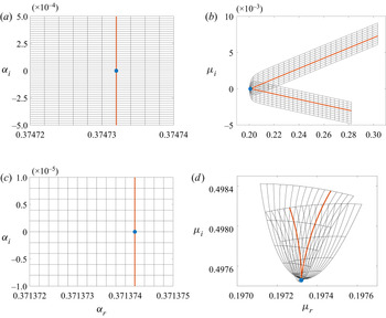
 $\mu _r$ in figure 8(b) and table 1. Figure 9 depicts the two types of cusps that emerge, in which the imaginary part of the Floquet exponent
 $\mu$ is zero and a half, respectively. The two cusp formations were constructed by first locating regions within the stability parameter space that for
 $\alpha \in \mathbb {R}$ establish the least-stable Floquet mode
 $\mu$, with the imaginary part
 $\mu _i=0$ or
 $\mu _i=1/2$. The complex
 $\alpha$-plane was then divided into a rectangular mesh grid about this point, as indicated by the horizontal and vertical black lines in figure 9(a,c). A very fine resolution was implemented, with step sizes
 ${\rm \Delta} \alpha _r = 10^{-7}$ and
 ${\rm \Delta} \alpha _i = 10^{-8}$ along the respective horizontal and vertical directions. As shown in figure 9(b,d), each grid point was then mapped via the solution to (3.10) onto the complex
 $\mu$-plane. Those grid lines nearest to the cusps (in the complex
 $\mu$-plane) are indicated by the red lines, with the cusp locations marked by the circular blue markers. The corresponding grid lines in the complex
 $\alpha$-plane are given by the vertical red lines. In both instances, the cusp is matched to a real-valued wavenumber
 $\alpha$ (circular blue markers in figure 9a,c), while the real part of the Floquet exponent
 $\mu$ is positive, i.e.
 $\mu _r>0$. Hence, by the symmetry arguments of § 4.3, pointwise growth occurs, which demonstrates that the Stokes layer is absolutely unstable for
 ${Re}=750$.
Rectangular mesh grids in the complex  $\alpha$-plane (a,c) are mapped via the dispersion relation
 $D(\alpha _0,\mu _0) = 0$ onto the complex
 $\mu$-plane (b,d), revealing cusp formations. The cusp in (b) corresponds to
 $\mu _i = 0$ and the tip of a finger-like protrusion (as indicated in figure 10), while the cusp in (d) corresponds to
 $\mu _i = 1/2$ and is located about the mid-point between two adjacent fingers.

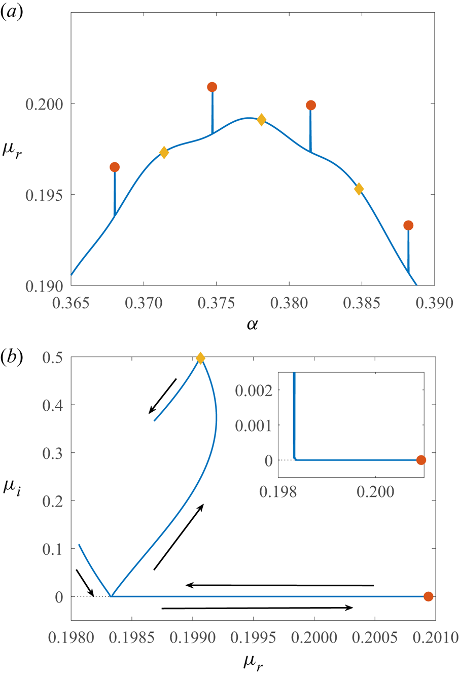
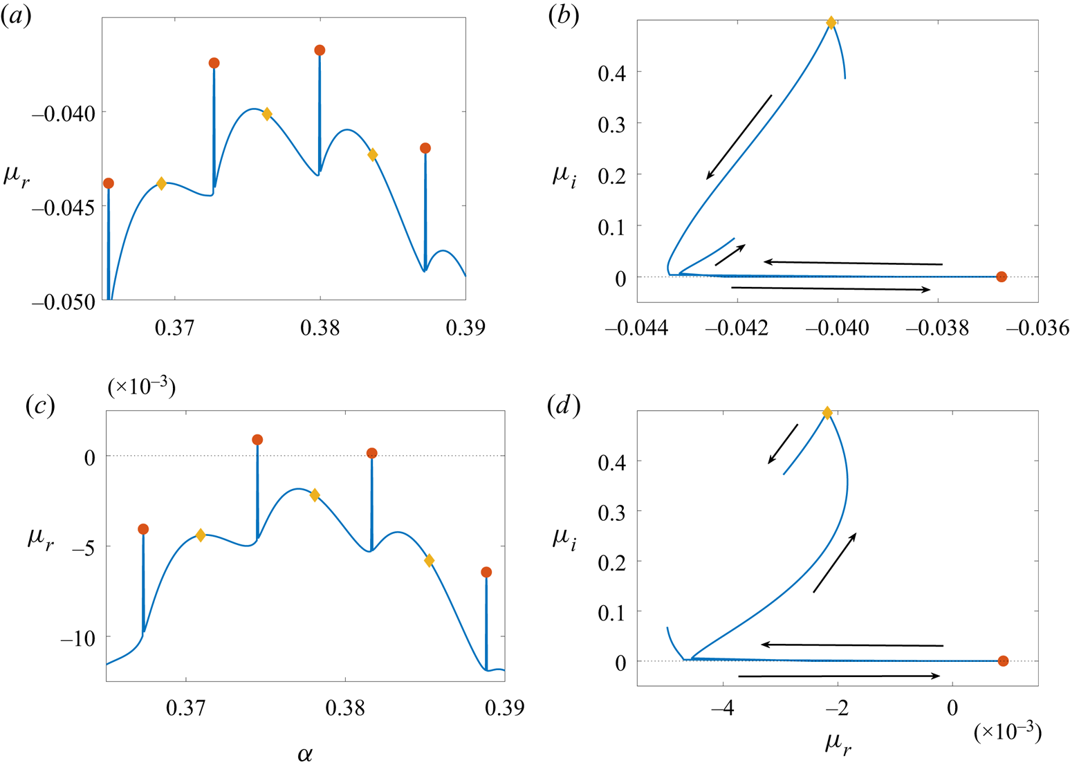
The cusp depicted in figure 9(b) corresponds to the tip of a finger-like protrusion in figure 8(b), where  $\mu _i=0$. For visual clarity this is re-plotted over a reduced wavenumber
 $\alpha$-range in figure 10(a). This particular mode exhibits the greatest Floquet growth rate for the given Reynolds number:
 $\mu _r=0.2009$ and
 $\alpha =0.3747$. Hence, as
 $\mu _i=0$ and
 $\mu _r>0$, harmonic growth occurs for this particular parameter set. Further harmonic cusps, with
 $\alpha _i = \mu _i = 0$, were located about the tips of other finger-like protrusions, as demonstrated in figure 10(a) (red circular markers).
(a) Floquet growth rate  $\mu _r$ as a function of the wavenumber
 $\alpha \in \mathbb {R}$ for the Reynolds number
 ${Re} = 750$. Same as figure 8(b) but over a reduced
 $\alpha$-range. (b) Path of the least-stable mode in the complex
 $\mu$-plane, for
 $\alpha \in [0.374,0.379]$. (Arrows indicate the direction of increasing
 $\alpha$.) Red circular and yellow diamond markers indicate those locations matched to absolutely unstable harmonic and subharmonic modes, where
 $\mu _i=0$ and
 $1/2$, respectively.

The illustration in figure 9(d) displays a cusp with  $\mu _i \approx 1/2$ and is associated with subharmonic growth. Here
 $\mu _r=0.1973$ and
 $\alpha =0.3714$. Several additional subharmonic modes are indicated by yellow diamond markers along the curve in figure 10(a). Furthermore, these particular modes are located about the mid-point between adjacent finger-like protrusions. Hence, the pointwise growth of the disturbance, established for the Reynolds number
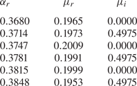
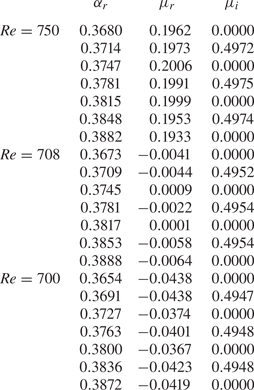
 ${Re}=750$, is characterised by a set of both harmonic and subharmonic absolutely unstable modes. The location of all cusps found by the construction of the cusp-map diagrams, similar to figure 9, are reported in table 2. (Note that the cusp associated with the subharmonic mode,
 $\mu _i\approx 1/2$, is not found at exactly
 $\mu _i=1/2$. Further discussion on this particular observation is included in § 5.4.)
Real part of the wavenumber  $\alpha$ (with
 $\alpha _i=0$) and Floquet exponents
 $\mu =\mu _r+\textrm {i}\mu _i$, associated with cusps for
 ${Re}=750$. Cusps are indicated in figure 10 by circular and diamond markers.

The four harmonic (red circles) and three subharmonic (yellow diamond) modes marked in figure 10(a) are the only absolutely unstable modes found using the cusp-map method for the given range of wavenumbers  $\alpha$. Further cusps that establish absolute instability were located for smaller and larger valued
 $\alpha$, at regular
 $\alpha$-steps, but at smaller growth rates
 $\mu _r$. All remaining modes depicted along the blue curve in figure 10(a) are matched to convectively unstable behaviour characterised by disturbances that propagate to the left or right only.
The distinction between convectively and absolutely unstable behaviour in the context of the time-periodic Stokes layer is made by comparing the development of the disturbance streamfunction  $\psi$. In figure 11, contours of the real part of
 $\psi$ are plotted in the
 $(\tau /2{\rm \pi} ,y)$-plane, for four successive wavenumbers
 $\alpha =0.3731$,
 $0.3747$,
 $0.3764$ and
 $0.3781$, with the imaginary part of the Floquet exponent
 $\mu _i=0.25$,
 $0$,
 $0.25$ and
 $0.4975$, respectively. In each instance, the real part of the Floquet exponent is positive, leading to strong temporal growth. Additionally, each solution has been normalised on its respective maximum complex-valued amplitude
 $|\psi |$, while red and blue contours are matched to positive and negative valued
 $\psi _r$, respectively. Moreover, the corresponding solutions for the complex conjugate (with
 $\mu _i<0$) bring about a time shift of
 ${\rm \pi}$ along the time axis.
All four plots share several common characteristics, consistent with the observations first made by Blennerhassett & Bassom (Reference Blennerhassett and Bassom2002) and subsequently by Thomas (Reference Thomas2020, Reference Thomas2021). For the four parameter settings considered, perturbations first appear within the boundary layer about either  ${\rm \pi} /4\leq \tau _1\leq {\rm \pi}/2$ or
 $5{\rm \pi} /4\leq \tau _2\leq 3{\rm \pi} /2$. (The subscript
 $1$ and
 $2$ notation in
 $\tau$ has been introduced here to indicate the first or second time interval that disturbances emerge during the periodic cycle.) Initially, each disturbance evolves with a high-frequency oscillation and grows along lines of constant
 $\tau -y$. A maximum amplitude is then realised near the boundary layer edge, about either the mid-point or endpoint of the cycle that are matched to the wall velocity (2.1) achieving either a minimum or maximum. Further away from the wall, the disturbance diminishes and the frequency of oscillation decreases.
As noted by Blennerhassett & Bassom (Reference Blennerhassett and Bassom2002), the upper bound on the time intervals  $\tau _1$ and
 $\tau _2$ coincides with the velocity (2.1) of the bounding plate being zero. Moreover, it was shown by Thomas et al. (Reference Thomas, Davies, Bassom and Blennerhassett2014) that perturbations grow rapidly when the wall shear stress
 $U'_B(0,\tau )$ changes sign (see figure 1 of their paper). A negative to positive change in
 $U'_B(0,\tau )$ occurs at
 $\tau ={\rm \pi} /4$ and coincides with a disturbance propagating to the right, while a left-travelling disturbance appears at
 $\tau =5{\rm \pi} /4$ when
 $U'_B(0,\tau )$ reverses from a positive to a negative value. Hence, given these observations, disturbances for
 $\alpha =0.3731$ and
 $\alpha =0.3764$, plotted in figures 11(a) and 11(c), are found to propagate to the right and left, respectively. Thus, these particular travelling modes display convectively unstable characteristics, as they propagate in one direction only. (This is true for all modes with
 $0<\mu _i\lessapprox 0.5$.) On the other hand, for the harmonic
 $(\alpha ,\mu _i)=(0.3747,0)$ and subharmonic
 $(\alpha ,\mu _i)=(0.3781,0.4975)$ modes plotted in figures 11(b) and 11(d), perturbations emerge about both time intervals
 $\tau _1$ and
 $\tau _2$, establishing disturbance development along both the left and right
 $x$-directions. Thus, the streamfunction
 $\psi$ further demonstrates the significance of these particular modes in establishing absolutely unstable behaviour in the Stokes layer. Note that the behaviour of these two modes is still classified as harmonic and subharmonic when the full normal mode structure (3.2) has been accounted for, i.e. solutions in figure 11 are scaled by
 $\exp (\mu \tau )$.
Contours of the real part of the disturbance streamfunction  $\psi$ over one period, for the Reynolds number
 ${Re}=750$; (a)
 $\alpha =0.3731$ and
 $\mu =0.1976+\textrm {i}0.2500$, (b)
 $\alpha =0.3747$ and
 $\mu =0.2009$, (c)
 $\alpha =0.3764$ and
 $\mu =0.1988+\textrm {i}0.2500$ and (d)
 $\alpha =0.3781$ and
 $\mu =0.1991+\textrm {i}0.4975$. Each disturbance is normalised on its respective maximum complex-valued amplitude.

The time interval that travelling modes  $0<\mu _i\lessapprox 0.5$ develop and the associated propagation direction is found to reverse as the wavenumber
 $\alpha$ increases. About the harmonic modes, the time interval changes from
 $\tau _1$ to
 $\tau _2$, leading to disturbances reversing direction and propagating from right to left. The opposite behaviour occurs near the subharmonic modes, with a
 $\tau _2$ to
 $\tau _1$ and left to right reversal taking place.
5.2.2. Approach II: $\alpha \in \mathbb {R}$

By constructing cusp-map diagrams, we have confirmed the existence of cusps in locations predicted by the symmetry arguments of § 4.3, for the Reynolds number  ${Re}=750$. However, extending the cusp analysis to other Reynolds numbers is computationally demanding, as (3.10) must be solved many times in order to fully resolve curves in the complex
 $\mu$-plane. (Recall that step sizes
 ${\rm \Delta} \alpha _r = 10^{-7}$ and
 ${\rm \Delta} \alpha _i = 10^{-8}$ were used to construct the mesh grid in figure 9(a,c).) Nevertheless, an alternative approach was implemented that allowed cusp locations to be determined more efficiently. Given the arguments presented in § 4.3 and those solutions tabulated in table 2, we restrict the cusp analysis to
 $\alpha _i = 0$, with real wavenumber step sizes
 ${\rm \Delta} \alpha _r=2\times 10^{-5}$; cusp locations are determined for
 $\alpha \in \mathbb {R}$ only. For instance, figure 10(b) depicts the path of Floquet modes in the complex
 $\mu$-plane for wavenumbers
 $\alpha \in [0.374,0.379]$, with arrows indicating the direction that
 $\alpha$ increases. The location of the most unstable harmonic and subharmonic cusps are then highlighted by circular and diamond markers, respectively. A smaller wavenumber step size
 ${\rm \Delta} \alpha _r=10^{-8}$ was implemented for the inset plot in figure 10(b), to fully resolve the behaviour near
 $\mu _i=0$. This approach was used to locate the rightmost harmonic cusp in figure 10(a), which was not reported in table 2 using the cusp-map approach. The cusps found using this faster approach are given in table 3, with calculations in excellent agreement with those results presented in table 2.
Location of cusps, as determined via the faster approach, whereby all cusps are assumed to be matched to  $\alpha \in \mathbb {R}$, i.e.
 $\alpha _i=0$. Calculations for
 ${Re}=750$ are in excellent agreement with results presented in table 2 that were based on the slower approach for locating cusps, i.e. wavenumbers
 $\alpha$ were allowed to be complex. Cusp locations are indicated by circular and diamond markers in figures 10 and 12.

The pointwise growth of the linear disturbance with  ${Re}=750$ is characterised by those harmonic and subharmonic modes marked in figure 10(a) and tabulated in tables 2 and 3. Although the leading-order behaviour, for large time
 $\tau$, is governed by the single least-stable mode, we do not expect this mode to dominate over a finite time period, as the harmonic and subharmonic modes develop with growth rates
 $\mu _r$ of commensurate size. Thus, for small time
 $\tau$ pointwise growth is described by a linear superposition of the multiple harmonic and subharmonic absolutely unstable modes. Since the superposition of harmonic and subharmonic modes is itself subharmonic, pointwise growth of the linear disturbance is subharmonic. This behaviour is consistent with the DNS computations presented in Ramage et al. (Reference Ramage, Davies, Thomas and Togneri2020) for the spatio-temporal disturbance development; during at least the first 10–20 periods of wall motion the disturbance amplitude, about fixed spatial
 $x$-locations, grows every two cycles of wall motion. In their study, Ramage et al. (Reference Ramage, Davies, Thomas and Togneri2020) found that subharmonic pointwise growth was brought about by the coalescence of two distinct wavepackets, the mother and granddaughter, in the spatio-temporal plane.
The harmonic modes depicted in figure 10 coincide with the local maxima of the Floquet growth rates  $\mu _r$. In particular, the most unstable of these harmonic modes lies on the global maximum that characterises the growth of the disturbance maximum (recall table 1). Thus, the pointwise growth of the disturbance, for large time
 $\tau$, is equal to the growth of the disturbance maximum. This particular observation is a key result from the earlier DNS investigation by Ramage et al. (Reference Ramage, Davies, Thomas and Togneri2020) (see figure 5 of their paper). Although such behaviour might be expected of a flow with no distinct upstream/downstream directions, it may appear somewhat at odds with the DNS computations reported in Thomas et al. (Reference Thomas, Davies, Bassom and Blennerhassett2014). In their study, that was limited to the first three periods of wall motion, Thomas and co-workers observed asymmetric behaviour that favoured the direction dictated by the time at which the impulsive forcing was applied. However, the longer time simulations generated by Ramage et al. (Reference Ramage, Davies, Thomas and Togneri2020) revealed that eventually the disturbance develops in a manner such that the pointwise growth is equivalent to that along the disturbance maximum.
Having shown that absolutely unstable behaviour arises for the Reynolds number  ${Re} = 750$, and that cusp locations of the dispersion relation
 $D(\alpha ,\mu ) = 0$ are consistent with the DNS results of Ramage et al. (Reference Ramage, Davies, Thomas and Togneri2020), we undertake an equivalent study for
 ${Re}=700$ and
 ${Re}=708$. The former case,
 ${Re} = 700$, is matched to a disturbance that is linearly stable for all wavenumbers
 $\alpha$, as demonstrated by the negative valued Floquet growth rates
 $\mu _r$ in figure 8(a). In figure 12(a), the growth rate
 $\mu _r$ is plotted over a reduced range of
 $\alpha$, near the local maximum growth rate (cross marker in figure 8a). Once again the Floquet growth rate
 $\mu _r$ is characterised by regular finger-like protrusions, with harmonic cusps (
 $\mu _i = 0$) located at the tips of each finger and subharmonic cusps (
 $\mu _i = 0.5$) located about the mid-point between adjacent fingers. All cusps were located using the faster approach, whereby Floquet growth rates were traced in the complex
 $\mu$-plane for real-valued
 $\alpha$, as demonstrated in figure 12(b) for the least-stable cusps (both harmonic and subharmonic) and reported in table 3.
Equivalent to figure 10 but for (a,b)  ${Re} = 700$ and (c,d)
 ${Re} = 708$. Floquet growth rate
 $\mu _r$ as a function of the real wavenumber
 $\alpha$ in (a,c). Paths of the most unstable Floquet modes
 $\mu$ in the complex
 $\mu$-plane in (b,d). Arrows indicate direction of increasing
 $\alpha$. Red circular and yellow diamond markers indicate those locations matched to harmonic (
 $\mu _i=0$) and subharmonic modes (
 $\mu _i=1/2$), respectively.

Unsurprisingly, all modes contributing to the pointwise development of the disturbance at  ${Re} = 700$ are stable, i.e.
 $\mu _i < 0$. However, since the behaviour is analogous to that described above for the Reynolds number
 ${Re} = 750$, we note that: pointwise evolution is dictated by a superposition of harmonic and subharmonic modes with comparable growth rates
 $\mu _r$. Thus, initially, the pointwise development is subharmonic. Additionally, the location of the least-stable cusp is matched to the local maximum that dictates the growth of the disturbance maximum. Hence, the pointwise growth and the growth along the disturbance maximum are identical. These observations are again consistent with the disturbance characteristics reported in Ramage et al. (Reference Ramage, Davies, Thomas and Togneri2020).
Given the above observations for both a strongly unstable ( ${Re} = 750$) and stable disturbance (
 ${Re} = 700$), where the pointwise growth is found to be equal to the growth along the disturbance maximum, it would be natural to assume that the onset of instability coincides with the onset of absolutely unstable behaviour. In order to demonstrate the veracity of this conjecture we consider the disturbance established for the marginally unstable Reynolds number
 ${Re} = 708$. In figure 12(c), a small section of the Floquet growth rate
 $\mu _r$ curve is plotted, with two unstable harmonic modes found about the tips of two protruding fingers (marked by red circles). These particular modes are matched to those finger-like protrusions found along the neutral stability curve in figure 6(b). As before, cusp locations and their stability characteristics were determined by tracing Floquet modes in the complex
 $\mu$-plane for real wavenumbers
 $\alpha$; demonstrated in figure 12(d) for the most unstable mode, with cusp locations tabulated in table 3. The pointwise evolution is governed by two marginally unstable harmonic modes and several marginally stable harmonic and subharmonic modes. Thus, the initial pointwise evolution of the impulse response will again be subharmonic. Moreover, pointwise growth about fixed spatial locations is again equal to that found along the disturbance maximum; the local maximum growth rate
 $\mu _r$ is again found about the tip of a finger-like protrusion. Hence, the disturbance, for the marginally unstable Reynolds number
 ${Re}=708$, is absolutely unstable.
5.3. Spatial periodicity due to multiple absolutely unstable modes
At fixed streamwise  $x$-locations, the finite-time impulse response is a superposition of harmonic and subharmonic modes that satisfy the collision criteria. All such modes reported in table 3, for each given Reynolds number
 ${Re}$, are evenly spaced with respect to the wavenumber
 $\alpha$. This then imposes a spatial periodicity on the solution, which suggests that the spacing between absolutely unstable modes is related to the fixed spatial spacing observed numerically between distinct wavepackets of the family-tree formation (recall figure 1 and the observations of Thomas et al. Reference Thomas, Davies, Bassom and Blennerhassett2014; Ramage et al. Reference Ramage, Davies, Thomas and Togneri2020). Using DNS, Ramage et al. (Reference Ramage, Davies, Thomas and Togneri2020) determined that the spatial spacing
 $\varLambda$ between neighbouring (mother and daughter) wavepackets was governed by the Reynolds number
 ${Re}$ (see figure 2 of the aforementioned paper). Furthermore, Ramage and co-workers observed a staggered wavepacket pattern in the family-tree structure, whereby a
 $2\varLambda$ spatial periodicity develops between wavepackets of comparable magnitude (see figures 3 and 4 of their paper, the former reproduced here in figure 1).
The relationship between the spatial periodicity  $\varLambda$ of individual wavepackets (as determined via DNS) and the wavenumber spacing between harmonic/subharmonic modes is investigated here by measuring the latter for a range of Reynolds numbers
 ${Re}$. These measurements are then compared with the
 $\varLambda$ calculations presented by Ramage et al. (Reference Ramage, Davies, Thomas and Togneri2020). Given the above observations for
 ${Re} = 700$,
 $708$ and
 $750$, we assume that all harmonic/subharmonic modes are evenly spaced along the wavenumber
 $\alpha$-axis. Moreover, each mode alternates between harmonic behaviour at the finger tips and subharmonic behaviour at the mid-point between adjacent fingers. The wavenumber spacing
 ${\rm \Delta} \alpha ^f$ between finger protrusions is then readily computed for each Reynolds number
 ${Re}$, without the construction of the numerically expensive cusp diagrams or the significant numerical resolution required to observe the cusp behaviour in the complex
 $\mu$-plane. The distance between harmonic and subharmonic modes is then assumed to be half the distance between two adjacent fingers:
 ${\rm \Delta} \alpha ^f/2$. Since the evolution at fixed spatial locations consists of a discrete set of evenly spaced modes, we anticipate a spatial periodicity of
 $4 {\rm \pi}/ {\rm \Delta} \alpha ^f$ between wavepackets of comparable magnitude. Thus, given the observation by Ramage et al. (Reference Ramage, Davies, Thomas and Togneri2020) that wavepackets of similar size are separated by a streamwise distance
 $2\varLambda$, the following relationship between
 $\varLambda$ and
 ${\rm \Delta} \alpha ^f$ is formulated
 \begin{equation} 2\varLambda = \frac{4{\rm \pi}}{{\rm \Delta} \alpha^f} \Rightarrow \varLambda = \frac{2 {\rm \pi}}{{\rm \Delta} \alpha^f}. \end{equation}
Hence, the streamwise distance  $\varLambda$ between each distinct wavepacket of the family-tree structure (i.e. between mother and daughter) is determined by the periodicity of the harmonic modes found at the tip of the finger-like protrusions.
The wavenumber spacing  ${\rm \Delta} \alpha ^f$ between neighbouring finger protrusions is computed for several Reynolds numbers
 ${Re}$, and in each instance,
 ${\rm \Delta} \alpha ^f$ is found to be constant. Black cross markers in figure 13 depict the corresponding spatial distance
 $2 {\rm \pi}/ {\rm \Delta} \alpha ^f$ as a function of
 ${Re}$, with the equivalent wavepacket spacing
 $\varLambda$ (determined using DNS by Ramage et al. Reference Ramage, Davies, Thomas and Togneri2020) plotted using red circles. The solid blue line depicts the line of best fit. Excellent agreement is achieved between the two independent calculations for all cases considered. A small difference, equivalent to
 $0.2\,\%$ of
 $\varLambda$, emerges for the Reynolds numbers
 ${Re} \geq 800$. However, this minor discrepancy is due to the approach in approximating
 ${\rm \Delta} \alpha ^f$ for these larger valued Reynolds numbers.
Spatial distance  $\varLambda$ between neighbouring wavepackets of the family-tree formation, as reported in Ramage et al. (Reference Ramage, Davies, Thomas and Togneri2020) (circle markers), and spatial distance
 $2 {\rm \pi}/ {\rm \Delta} \alpha ^f$ (cross markers) determined from the wavenumber distance
 ${\rm \Delta} \alpha ^f$ between finger-like protrusions along the real wavenumber
 $\alpha$-axis.

5.4. Discussion
Results presented in figures 9–12 and tables 2–3 suggest that there is a numerical inconsistency between where we expect the subharmonic cusps to occur and where they actually appear. The symmetry constraints, presented in § 4.3, indicate that subharmonic cusps correspond to  $\mu _i=0.5$. However, the above cusp analysis found them at a marginally smaller value near
 $\mu _i=0.497$. In an attempt to address this particular issue, the least-stable subharmonic cusp, for the Reynolds number
 ${Re} = 750$, was reproduced with an increasingly finer numerical resolution, with convergence to
 $\mu _i = 0.5$ anticipated. However, reducing the step size
 ${\rm \Delta} \alpha$ by several orders of magnitude had a negligible effect on those Floquet growth rates
 $\mu _i$ reported in tables 2 and 3. Further validation checks were carried out for both larger harmonics
 $N$ and the number of Chebyshev points along the wall-normal
 $y$-direction, but the cusp analysis remained unchanged. (Note that the corresponding harmonic cusps were always found for
 $\mu _i=0$, below any numerical tolerance.)
While this apparent inconsistency remains largely unexplained, it is important to emphasise that the location of these subharmonic cusps is consistent with the disturbance development reported by Ramage et al. (Reference Ramage, Davies, Thomas and Togneri2020). Hence, these cusps satisfy the collision criteria and are associated with the development of absolutely unstable behaviour.
6. Conclusions
The classification of linearly unstable behaviour in the time-periodic Stokes layer, as being convective or absolute, has been investigated using a modified form of the Briggs (Reference Briggs1964) method. The approach used herein was adapted from that implemented by Brevdo & Bridges (Reference Brevdo and Bridges1997) for temporally oscillating flows, with Floquet theory utilised to account for the periodicity of the flow. Given the antiperiodicity of the Stokes layer (2.2), symmetry constraints were derived that establish conditions for classifying linear disturbances as either convectively unstable or absolutely unstable. It was determined that the impulse response and pointwise development of the linear disturbances was dominated by those collisions that arose for wavenumbers  $\alpha \in \mathbb {R}$ and Floquet exponents
 $\mu = \mu _r + \textrm {i}k/2$, with
 $k=0$ and
 $k=1$. Harmonic and subharmonic behaviour was then matched to those modes with
 $k=0$ and
 $k=1$, respectively.
Symmetry arguments were coupled to the cusp-map method, developed by Kupfer et al. (Reference Kupfer, Bers and Ram1987), and used to locate absolutely unstable modes in the Stokes layer when the streamwise wavenumber  $\alpha \in \mathbb {C}$. The analysis was applied to the unstable disturbance that develops for the Reynolds number
 ${Re} = 750$, with 6 cusps located in the complex Floquet exponent
 $\mu$-plane. In each instance, the wavenumber
 $\alpha$ was real valued only. Three of these cusps were found about the tips of fingers that protrude from the growth-rate curves and correspond to
 $\mu _i = 0$, i.e. stationary waves. The remaining three cusps were located about the mid-point between adjacent fingers, with
 $\mu _i \approx 1/2$. Thus, cusp locations were matched to both harmonic and subharmonic behaviour. Hence, the pointwise growth of linear disturbances is characterised by subharmonic behaviour, which is consistent with the DNS computations presented by Ramage et al. (Reference Ramage, Davies, Thomas and Togneri2020); about fixed streamwise positions, the disturbance grows every two full periods of wall oscillation. Moreover, as the real part of the Floquet exponent
 $\mu$ was positive for each of these 6 cusps, the linear disturbance for
 ${Re}=750$ is classified as absolutely unstable.
Cusps in the complex  $\mu$-plane were only found for real-valued streamwise wavenumbers
 $\alpha$. The analysis was therefore extended to the respective stable and marginally unstable Reynolds numbers
 ${Re} = 700$ and
 ${Re} = 708$, with
 $\alpha \in \mathbb {R}$. Thus, the significant computational requirements in generating cusp-map diagrams was no longer necessary. As with the larger valued Reynolds number (
 ${Re}=750$), linear disturbances were again characterised by both harmonic and subharmonic modes. Furthermore, it was demonstrated that the Floquet mode with the largest growth rate, that dictates the growth of the disturbance maximum, coincides with the mode that dictates the pointwise growth of the disturbance. Thus, the growth rate about fixed spatial locations is identical to the growth rate of the disturbance maximum, which is consistent with the earlier DNS observations of Ramage et al. (Reference Ramage, Davies, Thomas and Togneri2020): the onset of linear instability in the Stokes layer, with the critical Reynolds number
 ${Re}_c=707.84$ (as first observed by Blennerhassett & Bassom Reference Blennerhassett and Bassom2002), coincides with the onset of absolutely unstable behaviour.
Finally, it was shown that the spatial periodicity imposed by the regular spacing of cusps with respect to the wavenumber  $\alpha$ is consistent with the periodic spatial spacing between wavepackets of the family-tree structure simulated numerically by Ramage et al. (Reference Ramage, Davies, Thomas and Togneri2020).
6.1. Future work
Following the earlier studies by Thomas et al. (Reference Thomas, Blennerhassett, Bassom and Davies2015) and Ramage et al. (Reference Ramage, Davies, Thomas and Togneri2020), a natural next step would be to extend the analysis to the family of flows established when the wall motion is modified via a low-amplitude, high-frequency noise. This family of flows would be of particular interest because, depending on the harmonic frequency of the noise-like modulation, it is possible to construct a flow that is not antiperiodic. In fact, it was reported by Ramage et al. (Reference Ramage, Davies, Thomas and Togneri2020) that for these non-antiperiodic flows, the pointwise growth rate is no longer equal to the growth rate of the disturbance maximum. Moreover, the disturbance develops a spatially asymmetric structure, while still exhibiting pointwise growth. The present framework would provide a solid theoretical foundation for these flows and for the reported breakdown of the family-tree structure, so long as a suitable method for testing the collision criteria is introduced for cases where the symmetry arguments are no longer valid (some preliminary results are outlined in Ramage Reference Ramage2017).
Acknowledgements
The authors wish to acknowledge the contributions of Dr P. Blennerhassett and Professor A. Bassom at the outset of this work. We are grateful to the referees for several suggestions which have led to a much improved paper.
Funding
This work was supported by the Engineering and Physical Sciences Research Council (EPSRC).
Declaration of interests
The authors report no conflict of interest.