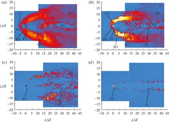
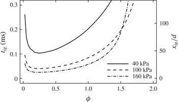
1. Introduction
A jet in crossflow is one of the most fundamental canonical flows for the investigation of turbulent mixing and combustion at both the fundamental and the applied level. It is of relative simplicity, yet it maintains many features of interest, such as three-dimensionality, separation and recirculation regions, wall-bounded effects and vortical flow regions. Furthermore, it has a level of practical relevance to engineering applications. A jet in crossflow can be found in many technological processes, from the industrial level (e.g. an industrial flare stack) to fuel delivery strategies in propulsion applications. A significant body of work has been conducted to characterize and study this system, at both low and high (i.e. supersonic) speeds, especially under non-reacting conditions. Two recent review articles on the study of transverse jets are by Karagozian (Reference Karagozian2010) and Mahesh (Reference Mahesh2013).
Transverse jets in crossflow (using hydrogen or other hydrocarbon fuels) have long been candidates as simple fuel delivery configurations in supersonic combustion engines (Huber, Schexnayder & McClinton Reference Huber, Schexnayder and McClinton1979). Arrays of single or staged injectors have in fact been proposed and investigated as fuel delivery strategies for air-breathing high-speed propulsion systems ranging from ramjet to scramjet engines. However, their limitations in flame-holding, fuel penetration and mixing characteristics are known in these applications; thus, other configurations that include various mixing-enhancement strategies have been considered (Gutmark, Schadow & Yu Reference Gutmark, Schadow and Yu1995; Seiner, Dash & Kenzakowski Reference Seiner, Dash and Kenzakowski2001) and continue to be developed. Some of the application-driven configurations are based on wall injection in the presence of a cavity (Donbar et al. Reference Donbar, Gruber, Jackson, Carter and Mathur2000; Rasmussen et al. Reference Rasmussen, Driscoll, Hsu, Donbar, Gruber and Carter2005; Rasmussen, Dhanuka & Driscoll Reference Rasmussen, Dhanuka and Driscoll2007; Ryan et al. Reference Ryan, Gruber, Carter and Mathur2009; Hsu et al. Reference Hsu, Carter, Gruber, Barhorst and Smith2010) or hyper-mixing configurations where vorticity-induced mixing is used to improve the overall performance and operability of supersonic combustors (Hartfield, Hollo & McDaniel Reference Hartfield, Hollo and McDaniel1994; Gauba et al. Reference Gauba, Klavuhn, McDaniel, Victor, Krauss and Whitehurst III1997; Doster et al. Reference Doster, King, Gruber, Carter, Ryan and Hsu2009; Vergine et al. Reference Vergine, Maddalena, Miller and Gamba2015).
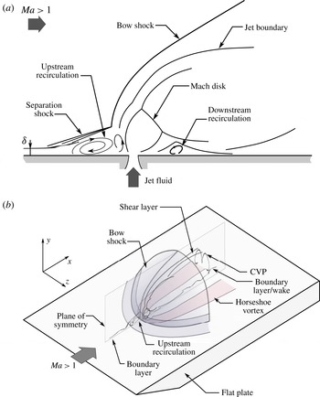
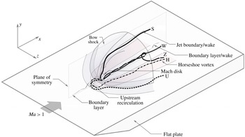
Many of the general flow properties of a jet in crossflow are also found in the supersonic counterpart – the jet in supersonic crossflow (JISCF). Low-speed transverse jets in crossflow are characterized by a complex system of vortical structures generated by the interaction of the transverse jet with the crossflow (Fric & Roshko Reference Fric and Roshko1994; Kelso & Smits Reference Kelso and Smits1995; Smith & Mungal Reference Smith and Mungal1998). The near field is characterized by horseshoe vortices that wrap around the base of the jet and by shear layer vortices that develop in the windward side of the transverse jet. The far field is dominated by a persistent counter-rotating vortex pair (CVP). The CVP forms in the near field by reorganization of shear layer vorticity into a folded vortex sheet that deflects in the far field to align (the axis of the CVP) with the direction of the crossflow (Kelso, Lim & Perry Reference Kelso, Lim and Perry1996; Cortelezzi & Karagozian Reference Cortelezzi and Karagozian2001). Finally, for sufficiently strong transverse jets, the wake of the jet is characterized by wake vortices that are generated near the wall and stretch towards the deflected jet (Fric & Roshko Reference Fric and Roshko1994). The supersonic counterpart retains some of these most important vortical structures. The main new contribution to the flow field comes with the formation of a complex system of shocks due to the supersonic crossflow (see the schematic diagrams of figure 1).
Schematic diagrams of a transverse jet in supersonic crossflow showing some of the dominant flow features: (a) side-view; (b) three-dimensional view showing the transverse jet injected from a flat plate.

A typical configuration used in the supersonic regime is to generate the transverse jet by underexpanded sonic injection at an angle (perpendicular, for example, as we consider in this study) to the supersonic crossflow from a surface. A large body of fundamental work has been directed at detailing the general structure and performance of this system (Dowdy & Newton Reference Dowdy and Newton1963; Schetz, Hawkins & Lehman Reference Schetz, Hawkins and Lehman1967; Billig, Orth & Lasky Reference Billig, Orth and Lasky1971; Cohen, Coulter & Egan Reference Cohen, Coulter and Egan1971; Povinelli & Povinelli Reference Povinelli and Povinelli1971; Papamoschou & Hubbard Reference Papamoschou and Hubbard1993; Gruber et al. Reference Gruber, Nejad, Chen and Dutton1996), its flow field and mixing characteristics (Rogers Reference Rogers1971b ; Gruber et al. Reference Gruber, Nejad, Chen and Dutton1995; Santiago & Dutton Reference Santiago and Dutton1997; Everett et al. Reference Everett, Woodmansee, Dutton and Morris1998; Gruber & Goss Reference Gruber and Goss1999; VanLerberghe et al. Reference VanLerberghe, Santiago, Dutton and Lucht2000; Kobayashi et al. Reference Kobayashi, Bowersox, Srinivasan, Carter and Hsu2007), the effect of the boundary layer (Dowdy & Newton Reference Dowdy and Newton1963; McClinton Reference McClinton1974) and injection details (e.g. angle, staging, etc.) (Bier, Kappler & Wilhelmi Reference Bier, Kappler and Wilhelmi1971; McDaniel & Graves Reference McDaniel and Graves1988; Hollo, McDaniel & Hartfield Reference Hollo, McDaniel and Hartfield1994; Hartfield & Bayley Reference Hartfield and Bayley1995).
Similarly to underexpanded jets in quiescent environments (Crist, Sherman & Glass Reference Crist, Sherman and Glass1966; Schetz et al. Reference Schetz, Hawkins and Lehman1967), transverse underexpanded jets form a complex system of expansion and shock waves (referred to as the barrel shock) as the jet expands into the crossflow. The barrel shock is deformed by the hydrodynamic forces resulting from the interaction with the incoming crossflow. A shear layer forms at the boundary between the deflected barrel shock and the crossflow. The flow blockage provided by the jet induces a three-dimensional bow shock that wraps around the transverse jet. For sufficiently large penetration of the jet, the bow shock is nearly normal at the base and folds around the jet resulting in diminishing strength. The bow shock stabilizes upstream of the jet and generates a rise in wall pressure upstream of the jet. When this pressure rise is larger than three times the undisturbed (free stream) value, the boundary layer separates (Dowdy & Newton Reference Dowdy and Newton1963) forming the upstream recirculation region which is characterized by two adjacent regions of swirling flow (Everett et al. Reference Everett, Woodmansee, Dutton and Morris1998): an upstream bubble associated with the boundary layer followed by a downstream one resulting from the presence of the jet. A three-dimensional separation oblique shock is also generated as a response to the upstream separation region. The separation and bow shocks intersect somewhere at the jet. The details of the upstream separation region depend on the characteristics of the incoming boundary layer (e.g. laminar or turbulent) and the size of the transverse jet (e.g. diameter). For instance, the pressure rise in the separation region in a laminar boundary layer is lower than in a turbulent boundary layer, although its length is larger by approximately a factor of three (Dowdy & Newton Reference Dowdy and Newton1963). Finally, because of the three-dimensionality of the bow shock, the incoming boundary layer experiences a three-dimensional interaction with the bow shock that extends further away from the immediate vicinity of the injector itself.
Many parameters describing the incoming crossflow and the jet itself are found to be important in describing the system. For example, the ratio of the boundary-layer thickness to the jet exit diameter is an important quantity to describe near-field events (McClinton Reference McClinton1974). The primary global flow-controlling parameter is the jet-to-crossflow momentum flux ratio, defined as
 $$\begin{eqnarray}J=\frac{{\it\rho}_{j}U_{j}^{2}}{{\it\rho}_{a}U_{a}^{2}}=\frac{p_{j}{\it\gamma}_{j}Ma_{j}^{2}}{p_{a}{\it\gamma}_{a}Ma_{a}^{2}},\end{eqnarray}$$
where
 ${\it\rho}$
and
 $U$
are the fluid density and speed respectively,
 $Ma$
is the Mach number,
 $p$
is the static pressure and
 ${\it\gamma}$
is the ratio of specific heats. The subscripts ‘
 $a$
’ and ‘
 $j$
’ refer to crossflow and jet bulk conditions respectively. Normally, the conditions describing the jet properties in (1.1) are taken at the jet exit. This parameter controls the overall penetration and spreading of the JISCF. A modification to the above relation based on the concept of an ‘effective back pressure’ can also be introduced to describe the initial near-field structure of the barrel shock (such as its size, height of the Mach disk and mass average properties along the centreline; Schetz & Billig Reference Schetz and Billig1966; Billig et al.
Reference Billig, Orth and Lasky1971).
Because of the performance limitations associated with mixing in supersonic combustion (Ferri Reference Ferri1973), mixing in the JISCF has been a primary focus of previous work (Rogers Reference Rogers1971a ,Reference Rogers b ; Torrence Reference Torrence1971; McDaniel & Graves Reference McDaniel and Graves1988; Gruber et al. Reference Gruber, Nejad, Chen and Dutton1995; Santiago & Dutton Reference Santiago and Dutton1997; VanLerberghe et al. Reference VanLerberghe, Santiago, Dutton and Lucht2000; Lin et al. Reference Lin, Ryan, Carter, Gruber and Raffoul2010). Many global morphological metrics such as the jet penetration have been defined and studied in these mixing studies. These studies have identified the importance of the windward shear layer on the entrainment process, along with the role of the CVP in the entrainment process in the wake. Because of the important role large-scale coherent structures play in the scalar transport processes, a large amount of work has been dedicated to understanding their dynamics and interaction with the supersonic crossflow (Gruber et al. Reference Gruber, Nejad, Chen and Dutton1996, Reference Gruber, Nejad, Chen and Dutton1997b ; Ben-Yakar, Mungal & Hanson Reference Ben-Yakar, Mungal and Hanson2006). Furthermore, the effect of compressibility (measured by an increase in convective Mach number) on the evolution of large-scale structures and its implication for the observed decrease in mixing have also been investigated (Gruber et al. Reference Gruber, Nejad, Chen and Dutton1997a ). In recent years, large-eddy simulation (LES) has been an important tool for better understanding the mixing and dynamics of the JISCF (Génin & Menon Reference Génin and Menon2010; Kawai & Lele Reference Kawai and Lele2010; Peterson & Candler Reference Peterson and Candler2010).
Reacting transverse jets in the supersonic high-enthalpy regime have also received attention. Previous work has primarily focused on developing diagnostic capabilities for these flows (Allen et al. Reference Allen, Parker, Reineeke, Legner, Foutter, Rawlins and Davis1993; McMillin, Seitzman & Hanson Reference McMillin, Seitzman and Hanson1994) and on investigating the ignition and stability characteristics of hydrogen transverse jets (Yoshida & Tsuji Reference Yoshida and Tsuji1977; Lee et al. Reference Lee, McMillin, Palmer and Hanson1992; Rothstein & Wantuck Reference Rothstein and Wantuck1992; Ben-Yakar & Hanson Reference Ben-Yakar and Hanson1998; Heltsley et al. Reference Heltsley, Snyder, Cheung, Mungal and Hanson2007). More recently, work has also been directed at investigating the reacting characteristics of more complex fuel injection approaches that can be found in scramjet applications (Donbar et al. Reference Donbar, Gruber, Jackson, Carter and Mathur2000; Rasmussen et al. Reference Rasmussen, Dhanuka and Driscoll2007; Ryan et al. Reference Ryan, Gruber, Carter and Mathur2009). More recently, reacting transverse jets in subsonic crossflow have also found renewed interest (Huang & Chang Reference Huang and Chang1994; Grout et al. Reference Grout, Gruber, Yoo and Chen2011; Kolla et al. Reference Kolla, Grout, Gruber and Chen2012; Micka & Driscoll Reference Micka and Driscoll2012; Schaupp, Friedrich & Foysi Reference Schaupp, Friedrich and Foysi2012; Sullivan et al. Reference Sullivan, Wilde, Noble, Seitzman and Lieuwen2014).
In the current study, we consider a single isolated transverse hydrogen jet injected perpendicularly to a high-enthalpy supersonic crossflow characteristic of Mach 8 flight enthalpy (pressure of 40 kPa, temperature of 1400 K and Mach number of 2.4) generated with an expansion tube. The objective of the work is to investigate the effect of the momentum flux ratio on ignition, stability, and global and local combustion characteristics of the system at fixed free stream conditions. We make use of
 $\text{OH}$
planar laser-induced fluorescence (PLIF) to mark the instantaneous reaction zone over several planes along the principal orthogonal directions (primarily streamwise/wall-normal and streamwise/spanwise planes). This allows us to generate a detailed view of the three-dimensional reacting flow field. We particularly focus on analysing the instantaneous structure of the reacting flow near the wall, where most of the reaction and flame stabilization is observed to take place.
In the following sections, a description of the experimental configuration and flow diagnostics will first be given, followed by a description of the main observations on the flow field and flame structure. The importance of the flow features resulting from the interaction of the transverse jet with the supersonic crossflow on ignition, flame stabilization and flame structure will be discussed in the final sections.
2. Experimental facility and configuration
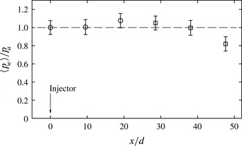
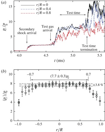
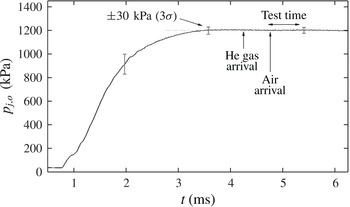
In this section, a description of the experimental facility, flow set-up and imaging configuration is given. A detailed description of the characterization of the flow condition produced by the expansion tube is reported in appendix A.
2.1. The expansion tube
The experiments presented here were conducted at the
 $6^{\prime \prime }$
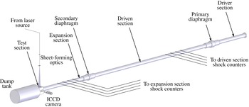
Expansion Tube Facility of the High Temperature Gas Dynamics Laboratory at Stanford University, which was used to generate the high-enthalpy supersonic crossflow used in the experiments. A schematic diagram of the expansion tube is shown in figure 2. An account of the design and operation of this facility is given by Heltsley et al. (Reference Heltsley, Snyder, Houle, Davidson, Mungal and Hanson2006); recent modelling efforts for this facility have been provided by Örley et al. (Reference Örley, Strand, Miller, Gamba and Iaccarino2011, Reference Örley, Gamba, Adams and Iaccarino2012). The operational principle and a theoretical analysis of the performance of an expansion tube to generate high-enthalpy supersonic and hypersonic flows can be found in the seminal work of Trimpi (Reference Trimpi1962). In brief, the expansion tube takes advantage of the unsteady shock and expansion waves produced in the tube to generate a short-duration (
 ${\sim}1~\text{ms}$
) supersonic high-enthalpy flow in the test section. The facility provides optical access for flow field imaging experiments.
Schematic diagram of the expansion tube showing the main sections, diaphragm assemblies, shock speed counters, and the flow laser illumination and imaging arrangement. The test section offers optical access on three sides.

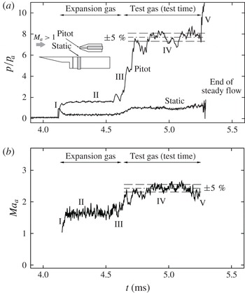
Calibration and characterization of the flow conditions generated by the expansion tube was performed using different approaches. All the results of these activities are described in appendix A. In brief, the calibration measurements established the following bulk-average free stream conditions for the experiment:
 $Ma_{a}=2.4$
,
 $p_{a}=40~\text{kPa}$
and
 $T_{a}\approx 1400~\text{K}$
(with a corresponding stagnation temperature of approximately 3000 K). The useful test time was approximately
 $500~{\rm\mu}\text{s}$
.
2.2. Transverse jet
The transverse jet was generated by issuing fuel perpendicularly to the crossflow from a flat plate. A three-dimensional schematic diagram of the flat plate configuration, along with some of the relevant flow features is shown in figure 1(b). The flat plate was composed of an aluminium plate with a hardened A-2 tool steel sharp leading edge (hardening of the leading edge was required to prevent damage during operation of the expansion tube). The resulting flat plate was approximately 155 mm (6.125 in.) long and 100 mm (4 in.) wide. The flat plate was mounted in the test section within the region of uniform and undisturbed supersonic flow bounded by the limiting characteristic region of the incoming flow and its inviscid core. A more detailed description of the flow characteristics of the incoming supersonic flow, including an assessment of temporal and spatial uniformity, is presented in appendix A.
Ultra-high-purity grade (99.999 % purity) hydrogen was used as fuel throughout the study. Fuel was injected from a contoured round injector with a
 $d=2~\text{mm}$
diameter and located on the centreline of the plate at approximately 64 mm from the leading edge. Fuel was delivered from a high-pressure gas cylinder, regulated by a pressure regulator, and delivered to the injector through high-pressure tubing. Fuel injection was controlled by a fast-acting solenoid valve (Valvetech model 15060-18) directly mounted beneath the flat plate at the plenum of the injector. To ensure a fully established flow to the injector, fuel injection was initiated at the beginning of the experiment well before the onset of the flow in the test section (see appendices A and B for further details). No active ignition device was used to ignite and stabilize the flame.
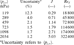
Six different jets generated at different jet stagnation pressures,
 $\langle p_{j,o}\rangle$
, under the same crossflow conditions were considered in the study. Some details about the calibration of the injector and the injection timing relative to the short-duration test are given in appendix B. The set of cases is summarized in table 1 and spans a range of momentum flux ratio,
 $J$
, from 0.3 to 5.0 at fixed free stream conditions. The values of
 $J$
were computed according to the definition (1.1) assuming isentropic expansion from
 $\langle p_{j,o}\rangle$
to sonic conditions and
 $p_{a}=40~\text{kPa}$
. It should be noted that the value of
 $\langle p_{j,o}\rangle$
reported in table 1 refers to the test time-averaged value of
 $p_{j,o}$
extracted from the calibration step. The jet exit Reynolds number,
 $Re_{d}={\it\rho}_{j}u_{j}d/{\it\mu}_{j}$
, based on the cold properties at the jet exit plane is also reported. The indicated uncertainty in table 1 refers to the uncertainty in
 $\langle p_{j,o}\rangle$
and accounts for both variation during the test time and measurement (calibration) uncertainty.
A direct quantification of the characteristics of the incoming boundary layer that develops on the flat plate was not possible. Schlieren imaging of the incoming flow (see later) suggests that the boundary layer remains thin, on the scale of approximately half jet diameter. Therefore, analytical results for supersonic laminar boundary layers (White Reference White1991) were used to estimate the boundary-layer thickness of the incoming flow. Under the free stream conditions of this study and assuming an isothermal wall near room temperature, the boundary-layer thickness was estimated to be approximately 1 mm. The unit Reynolds number of the incoming flow was approximately
 $3\times 10^{6}~\text{m}^{-1}$
and the local Reynolds number at the injector location was approximately
 $0.2\times 10^{6}$
. Under these conditions, a laminar boundary layer would be expected (White Reference White1991).
Summary of the hydrogen jet injection parameters:
 $J$
was computed assuming
 $p_{a}=40~\text{kPa}$
;
 $Re_{d}$
was computed based on the cold flow properties of hydrogen at the jet exit plane assuming choked conditions.

a
Uncertainty refers to
 $\langle p_{j,o}\rangle$
.
2.3. Imaging configuration
In the study, different imaging techniques were used to investigate the system: the flow and shock structure was visualized by Schlieren, the overall characteristics of the reacting jet were investigated by
 $\text{OH}^{\ast }$
chemiluminescence imaging, whereas the instantaneous reaction zone was visualized by
 $\text{OH}$
PLIF imaging.
The Schlieren system used in the study was a regular folded Z-type set-up. The illumination source was provided by a long-duration xenon flashlight, two 2 m focal length spherical mirrors were used to collimate and refocus the illumination source on the knife edge, and a LaVision ImagePro camera (resolution 1376
 $\times$
1040 pixel) was used for imaging. Background subtraction and normalization were performed on the acquired images. Instantaneous (500 ns exposure) and time-averaged (
 $20~{\rm\mu}\text{s}$
exposure) single-event images of the jet structure were acquired.
For the
 $\text{OH}$
PLIF imaging experiments, the
 $Q_{1}(N^{\prime \prime }=7)$
line near 283.3 nm of the
 $A^{2}{\it\Sigma}^{+}\leftarrow X^{2}{\it\Pi}(v^{\prime }=1,v^{\prime \prime }=0)$
electronic transition was selected. Broadband fluorescence from the whole upper excited state to all lower states was collected. The excitation source was provided by the frequency-doubled output of a tunable dye laser (Lumonics HD-500) pumped by a frequency-doubled Nd:YAG laser operated at 10 Hz (Continuum Powerlight 8000). The energy delivered was approximately 10 mJ per pulse. As shown schematically in figure 2, the excitation laser source was reflected towards the test section of the expansion tube and formed into a thin sheet by a combination of cylindrical lenses. The laser sheet thickness was estimated to be of the order of
 $300~{\rm\mu}\text{m}$
. A gated intensified CCD (ICCD) camera (Andor iStar, resolution
 $512\times 512$
pixels) fitted with a Nikon 105 mm,
 $f/4$
UV lens was placed perpendicularly to the illumination plane to collect fluorescence. UG-11 and WG-295 filters were used to reject unwanted light. The ICCD camera was gated to 400 ns to prevent interference of background illumination. Background subtraction and (mean) laser sheet non-uniform intensity correction was applied to the imaged fields. Laser energy shot-to-shot variation was also corrected for by monitoring the energy delivered during each imaging experiment. However, no attempt was made to correct for shot-to-shot variation of the laser sheet non-uniformity. Several side- and plan-view planes were considered. With reference to the coordinate system defined in figure 1(b), side-view planes are defined to be streamwise/wall-normal (
 $x$
–
 $y$
) planes, whereas plan-view planes are defined to be streamwise/spanwise (
 $x$
–
 $z$
) planes.
The
 $\text{OH}^{\ast }$
chemiluminescence imaging experiments used an imaging configuration very similar to the
 $\text{OH}$
PLIF experiments and differed only in the choice of spectral filter. For this case, a bandpass interference filter centred at 313 nm with a full-width at half-maximum of 10 nm was used on a similar ICCD camera configuration to that used for the
 $\text{OH}$
PLIF imaging. Only long-exposure (
 $200~{\rm\mu}\text{s}$
) imaging was considered to obtain a time-averaged and line-of-sight-integrated representation of the overall location of the burning regions. In this work, the
 $\text{OH}^{\ast }$
chemiluminescence is used as an approximate indicator of the global heat release distribution in the flow field. No calibration to relate heat release rate to emission intensity has been attempted and the reported results are used to draw conclusions based on a relative scale. Therefore, in order to allow for a direct comparison between different cases, the imaging configuration (such as magnification, field of view, etc.) and camera settings (such as gain on the intensifier, camera lens aperture, etc.) were maintained unaltered between all cases considered in the study. A discussion on the use of
 $\text{OH}^{\ast }$
chemiluminescence emission as a heat release rate indicator will be presented below.
To correctly interpret some of the results discussed below on the instantaneous structure of the reaction zone, it was necessary to describe the resolution of the imaging system used in the
 $\text{OH}$
PLIF experiments. Therefore, the modulation transfer function (MTF) of the imaging system was approximately constructed using the scanning knife-edge technique (Clemens Reference Clemens2002). A uniform white field was generated by an LED array placed behind a stack of ground glass plates and it was imaged with the ICCD camera as the knife edge was scanned across the field of view, from which the step-response function (SRF) was constructed at discrete points in the field of view. It was found that the SRF was well approximated by an error function, in which case the MTF is Gaussian. Knowledge of the MTF then allowed us to correct the length scales extracted from the
 $\text{OH}$
PLIF imaging following the method outlined by Wang & Clemens (Reference Wang and Clemens2004).
Due to the short duration of the available test time, all of the imaging experiments reported in this work are single-shot realizations repeated under nominally identical run conditions. Some of the composite figures showing the instantaneous flame structure reported in the following sections have been assembled from uncorrelated realizations. Furthermore, all of the single-shot imaging was carried out at the same nominal time delay with respect of the initiation of the flow (i.e. to the master trigger), well after a stationary flow was obtained. By taking
 $\text{OH}$
PLIF images at different time delays with respect to the master trigger, a (pseudo) time series of the instantaneous reaction zone was constructed (not shown) to assess transient effects leading to the stationary flow and to ensure that the remaining data were taken under stationary flow conditions. Similarly, kilohertz-rate
 $\text{OH}^{\ast }$
movies were taken to further assess the ignition transient. With reference to the pressure trace of figure 21 (shown in appendix A), the steady portion (of the pressure time trace) during the test time begins approximately
 $4.75~{\rm\mu}\text{s}$
from the master trigger, but a fully established stationary jet and flame structure is not observed until 4.9 ms. All imaging reported here has therefore been acquired well past this transient time. Thus, the
 $\text{OH}$
PLIF and Schlieren imaging was fixed at 5.1 ms, whereas the long-exposure
 $\text{OH}^{\ast }$
chemiluminescence imaging was initiated at 5.0 ms with a
 $200~{\rm\mu}\text{s}$
exposure.
3. Global structure and features of the reacting transverse jet
In this section the global characteristics of the reacting transverse jets are presented. First, the overall jet and shock structure as visualized by Schlieren imaging will be briefly presented. Then, the global burning and ignition characteristics as well as the far-field flame penetration and heat release distribution will be investigated from
 $\text{OH}^{\ast }$
chemiluminescence imaging. The detailed instantaneous flame structure as marked by the
 $\text{OH}$
radical will be investigated in the following section. The general flow and shock structure of a JISCF, and its dependence on the working parameters (such as
 $J$
), is now well known, as discussed earlier. However, because of its importance for the flame and stabilization characteristics that will be discussed below, a summarizing description for the particular cases under investigation is given first.
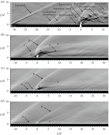
Schlieren images of the flow and shock structure around transverse underexpanded jets in supersonic crossflow: (a) instantaneous (500 ns exposure) Schlieren image for
 $J=5.0$
, (b) time-averaged (
 $20~{\rm\mu}\text{s}$
exposure) Schlieren image for
 $J=5.0$
, (c)
 $J=1.8$
and (d)
 $J=0.3$
; A, barrel shock; B, bow shock; C, separation shock; D, upstream separation region; E, recompression shock; F, shear layer; G, Mach wave.

3.1. Shock structure
The structure of the shock system for the case of the current experiments is shown in figure 3 where instantaneous (500 ns exposure) and time-average (
 $20~{\rm\mu}\text{s}$
exposure) Schlieren images are presented. The main characteristics have been outlined in the schematic diagram of figure 1 and correspond to the labelled features indicated in figure 3(a). In all figures presented here, the crossflow is from left to right. Figure 3(a) shows an instantaneous snapshot for the
 $J=5.0$
case. The image captures the incoming flow as it develops over the flat plate (indicated by the black outline) and the near field of the transverse jet. Well upstream of the injector, two shock wave systems are observed. First, a lip shock is formed by the interaction of the incoming supersonic flow with the boundary layer developing on the flat plate; second, a set of oblique waves is observed to originate from the flat plate (near
 $x/d=-15$
). The second shock wave system does not result from injection, nor does it originate by the mating of the sharp leading edge and the plate (which is near
 $x/d=-5$
). Its nature and origin could not be identified. However, it does not appear to interact with the transverse jet; thus, it is not expected to affect the jet. Figure 3(b) shows the corresponding time-average Schlieren image for the same case as figure 3(a). A few jet diameters upstream of the injector, the near field and part of the wake of the transverse jet are shown. Finally, figure 3(c,d) shows the time-averaged shock structure generated around the
 $J=1.8$
and
 $J=0.3$
cases.
The salient JISCF features that the Schlieren images identify are the bow shock (B) curving around the jet, the separation oblique shock (C), the deformed barrel shock (A) terminating in a tilted Mach disk, the recompression shock (E) at the lee side of the transverse jet following reattachment and the shear layer of the jet (F). Furthermore, these characteristics are strongly influenced by the value of
 $J$
. In particular, the penetration of the barrel shock increases with
 $J$
; similarly, the deflection and deformation of the barrel shock system is accentuated as
 $J$
is lowered until it disappears as it merges with the wake and boundary layer, as for the
 $J=0.3$
case, or until the subsonic limit is reached. The penetration of the jet into the crossflow provides flow blockage to the incoming flow, hence generating a three-dimensional bow shock whose strength depends on the level of blockage (i.e. the value of
 $J$
). The role and importance of the bow shock on the combustion characteristics will be emphasized further below when the global and instantaneous flame structure is discussed. One aspect to note here is the importance of the interaction of the bow shock with the incoming flow, especially with the boundary layer. As a result of the bow-shock/boundary-layer interaction, the incoming boundary layer separates (a process that is favoured with a laminar boundary layer; Dowdy & Newton (Reference Dowdy and Newton1963), Rogers (Reference Rogers1971a
,Reference Rogers
b
)) and a recirculation region forms in front of the jet (D). The recirculation region is visible in the
 $J=5.0$
case, but it is a fairly small feature in the
 $J=1.8$
and 0.3 cases. The strength and size of this flow feature are related to the strength of the interaction, which is controlled by the blockage-induced bow shock, hence
 $J$
. As a result of the recirculation region, a separation shock forms in front of the separation bubble (see figure 3
a). Both features play an important role in flame stabilization and flame holding (Dowdy & Newton Reference Dowdy and Newton1963; Schetz & Billig Reference Schetz and Billig1966; Schetz et al.
Reference Schetz, Hawkins and Lehman1967; Huber et al.
Reference Huber, Schexnayder and McClinton1979; Papamoschou & Hubbard Reference Papamoschou and Hubbard1993; Gruber et al.
Reference Gruber, Nejad, Chen and Dutton1996; Ben-Yakar & Hanson Reference Ben-Yakar and Hanson1998). The outline of the wake of the jet is visible downstream of the injection point and, past the recompression shock, it is not significantly affected by further shocks. In fact, the effect of the shock system generated by transverse injection is limited only in the near-field region as the flow is deflected by the jet, whereas the wake of the jet is relatively shock-free. This also implies that the pressure distribution in the wake of the (isolated) transverse jet quickly recovers to the undisturbed value, as surface pressure measurements have demonstrated (Everett et al.
Reference Everett, Woodmansee, Dutton and Morris1998; Gruber & Goss Reference Gruber and Goss1999). The details pointed out in this section have a role in the interpretation of the results drawn from the reaction zone imaging given further below; thus, they will be discussed further in the following sections. It should be noted that the weak wave labelled G in figure 3(c,d) is not associated with the separation shock, but it is a Mach wave emanating from the line joining the leading edge and the flat plate located at
 $x/d=-5$
. This Mach wave is visible only for cases with
 $J<3$
since the length of the upstream recirculation region is less than
 $5d$
; thus the flow can respond to this geometric feature by creating a Mach wave.
Line-of-sight integrated time-averaged
 $\text{OH}^{\ast }$
chemiluminescence imaging of the overall flame structure: (a)
 $J=0.3$
, (b)
 $J=1.8$
and (c)
 $J=5.0$
. For all cases the exposure was set to
 $200~{\rm\mu}\text{s}$
. The labels and lines are described in the text.

3.2. Global characteristics of the burning transverse jet
The overall ignition and flame characteristics of the system were investigated using
 $\text{OH}^{\ast }$
chemiluminescence imaging from naturally occurring chemically excited hydroxyl radicals as they decay from the
 $A^{2}{\it\Sigma}^{+}$
excited electronic state to the
 $X^{2}{\it\Pi}$
ground state through spontaneous radiative emission. The emitting excited species is generated by the chemical reaction process and it is limited by collisional quenching. Its emission intensity is related to the amount of the excited species. In premixed flames, for constant equivalence ratio, unburnt mixture temperature and heat losses, chemiluminescence has been shown to be an approximate direct indicator of the global heat release rate. However, its interpretation as an indicator of heat release rate is complicated by its dependence on turbulent fluctuations, strain rates, flame surface curvature and a weak dependence on unmixedness (Lee & Santavicca Reference Lee and Santavicca2003; Ayoola et al.
Reference Ayoola, Balachandran, Frank, Mastorakos and Kaminski2006). Because of these dependences, relating the emission intensity to the heat release rate is only approximate, especially in the context of non-premixed combustion as considered in the current study. Thus, chemiluminescence imaging is used in this study only for a qualitative description of the burning characteristics, their morphology and dependences. It should be noted that the approach followed in the present study provides a line-of-sight and time-integrated representation of the combusting flow field from a lateral view. Furthermore, multiple repetitions were compared to ensure repeatability in the average characteristics.
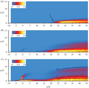
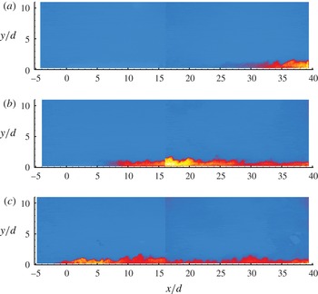
Examples of the time-averaged
 $\text{OH}^{\ast }$
chemiluminescence images (time integration of
 $200~{\rm\mu}\text{s}$
) are shown in figure 4 for transverse jets at (a)
 $J=0.3$
, (b)
 $J=1.8$
and (c)
 $J=5.0$
. The colourmap shown is linear and ranges from blue in the non-reacting regions to red and yellow in the reacting ones and terminates with white at the maximum intensity. To ensure that a meaningful comparison between the different cases can be made, the
 $\text{OH}^{\ast }$
imaging configuration and data reduction steps were the same for all injection cases, as also explained in § 2.3. Furthermore, the colourmap scale used in constructing figure 4 is the same for all cases presented here.
The integration time used in the
 $\text{OH}^{\ast }$
imaging experiments corresponds to more than 20 times the characteristic large-scale convective time scale,
 ${\it\tau}_{c}$
, of the system, which ensures convergence to a stationary (and shot-to-shot repeatable) representation of the combusting regions. The convective time scale
 ${\it\tau}_{c}$
is defined as
 $y_{o}/\overline{U}$
, which is the ratio between a characteristic large-scale length scale and the velocity scale of the system. The characteristic length scale
 $y_{o}$
is taken as the maximum jet penetration (for example, from the results of figure 3) observed within the field of view; the characteristic velocity scale
 $\overline{U}$
is taken as the arithmetic average between the free stream velocity (
 $U_{a}=1775~\text{m}~\text{s}^{-1}$
) and the jet exit velocity (
 $U_{j}=1250~\text{m}~\text{s}^{-1}$
). The choice of this velocity scale is motivated by the observation that the convective velocity of large-scale structures in JISCFs varies from
 $U_{j}$
near the injector to approximately
 $U_{a}$
as the wake-like region of the JISCF is approached (Gruber et al.
Reference Gruber, Nejad, Chen and Dutton1997a
; Ben-Yakar et al.
Reference Ben-Yakar, Mungal and Hanson2006).
Inspection of the set of images reveals that the characteristics of the overall burning regions, their structure and the stabilization points depend on the value of
 $J$
. The cases reported in figure 4 are selected to demonstrate the limiting behaviours that the study identifies. In particular, for values of
 $J<1$
(figure 4
a), it is observed that ignition does not occur at the injection point, but the flame is stabilized at some downstream point, which we refer to as the stabilization point
 $x_{s}$
, and it is indicated by the label A in figure 4(a) (
 $x_{s}$
will be defined formally further below). Furthermore, the burning region appears to be confined at the wall in a layer approximately
 $2d$
thick. As the Schlieren image of figure 3(c) qualitatively indicates, the
 $J=3$
case results in minimal fuel penetration into the crossflow (of the order of the boundary-layer thickness), and the wake of the jet remains attached to the wall.
As the value of
 $J$
is increased, the jet penetration increases and the stabilization point moves upstream. Nevertheless, the most intense burning region, as indicated by intense
 $\text{OH}^{\ast }$
emission, still remains confined to the near-wall wake region of the transverse jet. As the value of
 $J$
is raised above unity (see figure 4
b for the
 $J=1.8$
case), weak shear layer burning is detected by the
 $\text{OH}^{\ast }$
imaging and exists above the intense near-wall wake burning. For the
 $J=1.8$
case, near-field burning on the windward side of the transverse jet just behind the bow shock is also detected, but it is a weak feature.
Burning of the shear layer, either in the near field in the region of maximum deflection or downstream in the wake of the jet, becomes important only as
 $J$
is increased to values larger than
 ${\sim}3$
. As the value of
 $J$
is increased even further, the downstream stabilization point and the near-field burning merge and the reacting transverse jet is stabilized directly at the injector and upstream of it (see figure 4
c). However, even for the large value of
 $J$
considered in figure 4(c), the near-wall wake remains the region with the most intense burning as identified by the
 $\text{OH}^{\ast }$
emission. Furthermore, also for the
 $J=5.0$
case, there exists a region of low
 $\text{OH}^{\ast }$
emission downstream of the region of maximum deflection separating the near-field, post-bow-shock burning and the near-wall-stabilized wake combustion. This low-
 $\text{OH}^{\ast }$
-intensity region is interpreted as being the result of quenching of the shear layer due to the rapid expansion of the transverse jet which decreases its temperature and pressure, while it accelerates the flow and possibly increases straining of the mixing region. As a result, the rates of chemical reaction might decrease overall in this region until further downstream (
 $x/d>20$
) where temperature and pressure recover, and combustion can progress favourably. For
 $J$
larger than
 ${\sim}3$
, burning upstream of the injection point is observed (see figure 4
c). This feature has typically been associated with the upstream recirculation region which ignites and serves as a point of stabilization of the combustion process in the JISCF system (Huber et al.
Reference Huber, Schexnayder and McClinton1979) and has also been observed in previous work on reacting JISCF (Lee et al.
Reference Lee, McMillin, Palmer and Hanson1992; Ben-Yakar & Hanson Reference Ben-Yakar and Hanson1998).
As a concluding remark, it is important to point out that in all cases considered in the study most of the
 $\text{OH}^{\ast }$
chemiluminescence emission is detected close to the wall in the wake of the transverse jet, and, on average, emission in the shear layer is weaker, at least within the imaging region (up to 45 jet diameters downstream). Therefore, under the assumption that
 $\text{OH}^{\ast }$
emission tracks the heat release distribution, it appears that the region where most of the initial heat release occurs might be confined in the wake of the jet near the wall.
3.3. Flame lift-off
Assuming that the relative
 $\text{OH}^{\ast }$
luminosity can be taken as a marker of heat release, the results of figure 4 suggest that heat release might be negligible or completely absent in the near-field region for low values of
 $J$
(say
 $J<1$
). Thus, low-
 $J$
reacting transverse jets appear to be lifted similarly to low-speed jet and transverse jet flames. We define the stabilization point
 $x_{s}$
as the point downstream from the injector location where the first occurrence of
 $\text{OH}^{\ast }$
luminosity is observed. In extracting this quantity, to be consistent among all cases, the
 $\text{OH}^{\ast }$
images of figure 4 were first low-pass filtered (with a moving average filter of size
 $3\times 3$
pixels) and then thresholded to 10 % of the maximum value of the
 $\text{OH}^{\ast }$
signal observed in the full data set. The stabilization point
 $x_{s}$
is equivalent to the lift-off height or distance in low-speed flames. Depending upon the mechanisms responsible for stabilization at
 $x_{s}$
(discussed below), this distance could also be interpreted as an ignition delay distance (or time).
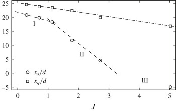
The stabilization point
 $x_{s}/d$
as a function of
 $J$
is shown in figure 5. Three different regions are identified in the figure and reflect the characteristics identified so far: (I) a region with a weak
 $J$
dependence where stabilization occurs in the wake of the jet, near the wall (
 $J<1$
), (II) a region where mixed wake and near-field shear layer ignition and stabilization occurs, and (III) a region where ignition and stabilization occurs upstream of the jet and a flame is maintained at all downstream locations (
 $J\gtrsim 3$
). Examples of the flame global structure consistent with each regime were shown in figure 4. In regime I,
 $x_{s}$
is a weak function of
 $J$
and approaches a limiting value of approximately
 $22d$
as
 $J\rightarrow 0$
. Values of
 $J<0.3$
were not investigated, therefore it is not known whether blow-off occurs and at what value of
 $J$
. For large values of
 $J$
in regime III, the reacting near-field shear layer, the upstream recirculation region and the wake burning regions merge together. It seems reasonable to expect that these features remain independent of
 $J$
at larger values.
In figure 5 we also identify a second quantity of interest, which we refer to as the location of heat release onset,
 $x_{q}$
, and, similarly to
 $x_{s}$
, it is reported as a function of
 $J$
. This quantity, which will be formally defined and discussed in more detail in § 3.5, indicates the point downstream of the injector where significant heat release takes place and linearly decreases with
 $J$
across the three regions (I, II and III) identified in figure 5 from
 $x_{s}$
. In general,
 $x_{q}$
is different from (and larger than) the stabilization point defined here; the latter defines where we first observe a stable flame irrespective of how much heat is locally released at the stabilization point, while the former defines where we first observe that a significant amount of heat has been released as a result of the combustion process. We will return to this quantity in § 3.5 when we discuss the distribution of heat release in the flow field.
The stabilization point (
 $x_{s}/d$
) and the location of heat release onset (
 $x_{q}/d$
) as a function of the momentum flux ratio
 $J$
.

3.4. Flame penetration
A second global characteristic is the penetration of the transverse jet flame into the crossflow. In this work, we define the penetration of the reacting jet based on the
 $\text{OH}^{\ast }$
imaging results. Because
 $\text{OH}^{\ast }$
was not detected in the near field of the transverse jet (for
 $x/d<20$
), penetration was defined only in the wake for
 $x/d>30$
and it was defined as the locus of points of the wall-normal location
 $(y)$
at which the
 $\text{OH}^{\ast }$
intensity was 10 % of the maximum intensity value. Because all cases considered in the study have the same distribution of values of
 $\text{OH}^{\ast }$
intensity, this definition is consistent for all cases and with the definition of
 $x_{s}$
.
(a) Penetration of the flame boundary for the cases considered in the study after
 $J$
-scaling (3.1) with the parameters
 $k$
and
 $m$
left to depend on
 $J$
. (b) Dependence of
 $m$
and
 $k$
on
 $J$
with best curve fit.

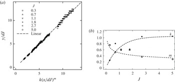
Figure 6(a) shows the extracted flame scaled penetration
 $y/d$
as a function of the scaled axial
 $x/d$
coordinate after
 $J$
-scaling. Penetration of jets in crossflow, in both the subsonic (Margason Reference Margason1993; Hasselbrink & Mungal Reference Hasselbrink and Mungal2001; Su & Mungal Reference Su and Mungal2004) and supersonic (Schetz & Billig Reference Schetz and Billig1966; Hersch, Povinelli & Povinelli Reference Hersch, Povinelli and Povinelli1970; Papamoschou & Hubbard Reference Papamoschou and Hubbard1993; Gruber et al.
Reference Gruber, Nejad, Chen and Dutton1995; Portz & Segal Reference Portz and Segal2006) regimes, is found to be primarily described by the parameter
 $J$
, although weak effects on boundary-layer thickness (McClinton Reference McClinton1974), crossflow Mach number (Portz & Segal Reference Portz and Segal2006) and jet fluid molecular weight (Ben-Yakar et al.
Reference Ben-Yakar, Mungal and Hanson2006) might be present. In constructing figure 6(a), it was assumed that the same holds for these reacting cases and for our definition of flame penetration. Thus, the flame penetration was scaled according to the following relation:
 $$\begin{eqnarray}\frac{y}{Jd}=k\left(\frac{x}{Jd}\right)^{m}.\end{eqnarray}$$
In the above relation, the values of the premultiplicative factor
 $k$
and of the exponent
 $m$
are allowed to vary with
 $J$
and are computed as a least-squares fit of (3.1) to the experimental observation. The
 $J$
-scaled results are shown in figure 6(a). For the range of
 $J$
values considered in the study, it is found that a relation of the type of (3.1) describes the flame penetration well, but with a somewhat strong dependence of
 $k$
and
 $m$
on
 $J$
. It should be noted that in constructing the best fit of figure 6(a), all possible parameters affecting penetration other than
 $J$
(e.g.
 ${\it\delta}/d$
,
 $Ma_{a}$
, molecular weight) are effectively held constant in this study (
 ${\it\delta}$
is the boundary layer thickness of the crossflow). Thus, if an extended model including these dependences were to be used, extra dependences would primarily be reflected on
 $k$
(Povinelli & Povinelli Reference Povinelli and Povinelli1971; McClinton Reference McClinton1974; Portz & Segal Reference Portz and Segal2006), but possibly also on
 $m$
.
Figure 6(b) shows the dependence of the parameters
 $k$
and
 $m$
on
 $J$
. It is found that
 $m$
varies from approximately 0.75 at low
 $J$
and approaches a limiting value of approximately 0.3 at large
 $J$
; similarly, it is found that
 $k$
varies from approximately 0.25 at low
 $J$
to a limiting value of approximately 1 at large
 $J$
. Furthermore, assuming that these two parameters would follow a
 $J$
scaling, best curve fits have been constructed and are presented in this figure. In particular, the premultiplicative factor is best correlated by
 $k=k_{\infty }(1-\text{e}^{Jq_{k}})$
with
 $k_{\infty }=1.05$
and
 $q_{k}\approx -1$
, and the exponent is best correlated by
 $m=m_{\infty }J^{q_{m}}$
with
 $m_{\infty }\approx 1/2$
and
 $q_{m}\approx -1/4$
. These functional forms are not supported on physical grounds, but are just proposed to conveniently correlated these parameters within the limited range of
 $J$
values considered in the study. The variation of
 $m$
and
 $k$
is possibly a consequence of the range of low values of
 $J$
considered in the study, and they approach limiting values for
 $J>5$
.
The penetration of low-speed (subsonic) constant-density transverse jets have been found to follow the form
 $$\begin{eqnarray}\frac{y}{rd}=A\left(\frac{x}{rd}\right)^{B},\end{eqnarray}$$
where
 $r=\sqrt{J}$
. This form has been successfully used to correlate a wide range of experimental observations (e.g. Margason Reference Margason1993) and it is consistent with conservation of momentum scaling arguments (e.g. Hasselbrink & Mungal Reference Hasselbrink and Mungal2001). Typical values for
 $A$
and
 $B$
are
 $A\approx 2$
and
 $B\approx 0.3$
. To reflect the use of
 $J$
, (3.2) can be written in a form similar to (3.1) with
 $k=AJ^{(B-1)/2}$
and
 $B=m$
. Assuming that the low-speed results apply to the supersonic regime, part of the variation of
 $k$
with
 $J$
could be attributed to a direct dependence of
 $J$
in the premultiplicative factor. However, the data in figure 6(b) indicate
 $\partial k/\partial J>0$
whereas (3.2) implies
 $\partial k/\partial J<0$
. Thus, the
 $J$
dependence of
 $k$
found here has to be attributed to an intrinsic dependence possibly due to the low value of
 $J$
. It is also interesting to note that for our case, the exponent tends to a limiting value of 0.3 for large
 $J$
as in the subsonic case.
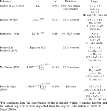
For the supersonic cases, the results of many studies support a functional form of the type of (3.1). The results of some of these studies are summarized in table 2 where the values of
 $k$
,
 $m$
and the conditions in those studies are reported. Previous studies have covered a relatively broad range of non-reacting conditions, but they all reduce to somewhat similar results. More notably, Povinelli & Povinelli (Reference Povinelli and Povinelli1971) studied the effect of different parameters and found that a more comprehensive relationship was the following (for
 $x/d^{\ast }>7$
):
 $$\begin{eqnarray}\frac{y}{d^{\ast }}=2.96\left(\frac{p_{o,jet}}{p_{eb}}\right)^{0.405}Ma_{j}^{0.163}\left(\frac{x}{d^{\ast }}+0.5\right)^{0.204}\left(\frac{{\it\theta}}{d^{\ast }}\right)^{0.141},\end{eqnarray}$$
where
 $d^{\ast }$
is the throat diameter,
 ${\it\theta}$
is the boundary-layer momentum thickness and
 $p_{eb}$
is the effective back pressure (Billig et al.
Reference Billig, Orth and Lasky1971). Their study, along with the ones by McClinton (Reference McClinton1974) and Portz & Segal (Reference Portz and Segal2006), emphasizes the importance of the boundary-layer thickness on penetration and entrainment. In particular, McClinton (Reference McClinton1974) found that
 ${\it\delta}/d$
has a weak effect on penetration defined as the 0.5 % jet concentration contour (see table 2); on the contrary, a stronger effect was found for jet penetration defined on the contour of local maximum concentration. In our study, the crossflow is held fixed, thus the boundary-layer thickness dependence cannot be assessed. Furthermore, our definition of penetration is more consistent with a definition based on the 0.5 % contour (since we are tracking regions near the stoichiometric contour), so we expect that overall the boundary layer would have a secondary effect, at least for sufficiently large values of
 $J$
(the work of McClinton (Reference McClinton1974) was carried out at a constant
 $J=1$
).
Summary of some of the transverse jet penetration results from non-reacting mixing studies. Unless otherwise noted,
 $Ma_{j}=1$
.
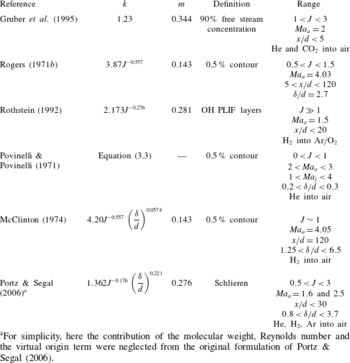
a For simplicity, here the contribution of the molecular weight, Reynolds number and the virtual origin term were neglected from the original formulation of Portz & Segal (Reference Portz and Segal2006).
All of the previous work indicates a similar dependence of the premultiplicative factor on
 $J$
but no dependence on the exponent. Our result is somewhat different since it gives the opposite dependence to what is typically observed. The discrepancy might be the result of the many different ways in which penetration has been defined and the different range of conditions considered (
 $Re$
,
 ${\it\delta}/d$
,
 $\mathscr{M}$
,
 $Ma_{a}$
,
 $x/d$
range, etc.).
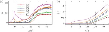
3.5. Heat release distribution
The
 $\text{OH}^{\ast }$
chemiluminescence distributions shown in figure 4 are here used as a proxy for the local heat release. Thus, the streamwise distribution of the heat release was marked by computing the streamwise distribution of the time-averaged
 $\text{OH}^{\ast }$
chemiluminescence intensity,
 $q(x/d)$
, from the images of figure 4. Specifically,
 $q(x/d)$
was computed by adding together the measured values of the
 $\text{OH}^{\ast }$
signal at all pixels along each column (i.e. for each one-pixel-wide column) in the image to generate a one-dimensional streamwise profile (i.e. by integrating the 2D distribution along the
 $y$
-direction without any integration in the
 $x$
-direction). This quantity was computed in the same way for all cases considered here. The resulting profiles are shown in figure 7(a). In general, we can observe a similar trend for all
 $J$
cases considered. For low-
 $J$
cases where ignition does not occur at the injector itself, the distribution of
 $q(x/d)$
first increases far downstream from the injector and shows a continuous increase up to a plateau; for the large-
 $J$
cases,
 $q(x/d)$
first peaks near the injector, decreases immediately downstream of the injector (flame quenching) and then
 $q(x/d)$
increases back to a plateau. The point where the plateau is reached moves upstream as
 $J$
increases, and the value of the plateau increases with
 $J$
.
The cumulative distribution of the heat release,
 $C_{q}(x/d)$
, was also computed and it is shown in figure 7(b) for the different cases. After the initial energy release that might exists directly at the injector, all
 $J$
cases show that the majority of the heat release occurs well downstream of the injection point with
 $C_{q}(x/d)$
increasing linearly with
 $x/d$
after the initial region (this is a result of the plateau observed in
 $q(x/d)$
). From the profiles of
 $C_{q}(x/d)$
we can also extract three more quantities: (i)
 $x_{q}$
, the point of heat release onset; (ii)
 ${\rm\Delta}C_{q}$
, the slope of
 $C_{q}(x/d)$
in the far field where the profile becomes linear; and (iii) the total energy released within the imaging region (i.e. the integral of
 $C_{q}(x/d)$
over
 $x/d$
). More specifically, the point of heat release onset is defined as the intercept on the
 $x$
-axis of the linear fit to
 $C_{q}(x/d)$
in the far-field linear portion – this definition is graphically shown in figure 7(b). One final quantity extracted from the
 $\text{OH}^{\ast }$
visualizations is the peak value of the
 $\text{OH}^{\ast }$
signal, which in all cases considered here occurs at a downstream location of approximately
 $x/d=30$
near the wall at a wall-normal location of less than
 $y/d=1$
(i.e. within what we can consider the boundary layer).
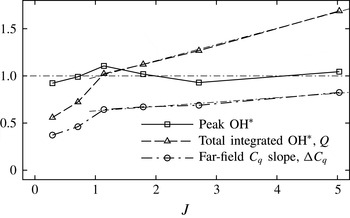
Three of these quantities (peak
 $\text{OH}^{\ast }$
,
 ${\rm\Delta}C_{q}$
, total integrated
 $q$
) are summarized in figure 8 as a function of
 $J$
, while
 $x_{q}$
is shown in figure 5 along with
 $x_{s}$
. It should be noted that in constructing these quantities the
 $\text{OH}^{\ast }$
was normalized so that the resulting quantities were of order 1 and could thus fit on the same scale. It is interesting to note that the peak
 $\text{OH}^{\ast }$
(i.e. peak local heat release rate) and the location where it occurs are the same for all cases considered as if the mechanism responsible for it remains invariant upon
 $J$
. As shown in figure 5,
 $x_{q}$
decreases linearly with
 $J$
from an extrapolated value of
 $x/d=25$
as
 $J\rightarrow 0$
to approximately
 $x/d=17$
for
 $J=5$
. Thus, although we observed that the point of first ignition (
 $x_{s}$
) moves to the injector as
 $J$
is increased, the point of heat release onset remains in the far field. Thus, the use of strong injection (i.e. high
 $J$
) can promote near-field flame stabilization, but it has a much weaker impact on the point where the majority of the heat release occurs (i.e.
 $x_{q}$
). The result also implies that in the transverse jet all of the heat release occurs far from the injector, thus requiring long combustion chambers to achieve complete combustion.
From the trends of the various quantities shown in figure 8, we can also observe that there are two regions characterized by a different dependence of the heat release distribution on
 $J$
. For
 $J\leqslant 1$
, there is a strong nonlinear variation of the parameters with
 $J$
. On the contrary, for
 $J>1$
, the dependence is linear. Simple energy balance considerations suggest that the cumulative heat releaser should increase linearly with
 $J$
(i.e. with the amount of fuel entering the system, thus
 $J$
since
 $U_{j}$
is constant). This is observed only for
 $J>1$
. Therefore, for low
 $J$
, other competing effects that prevent rapid and uniform chemical reaction must exist. This is possibly related to the stabilization process for low
 $J$
since a similar dependence is found for
 $x_{s}$
(figure 5).
(a) Normalized distribution of heat release
 $q(x/d)$
(arbitrary units) and (b) corresponding cumulative distribution
 $C_{q}(x/d)$
for different
 $J$
cases.


4. Instantaneous reaction zone structure
 $\text{OH}$
PLIF imaging is used to investigate the instantaneous structure of the reaction regions on several side- and plan-view planes. Different off-centreplane side-view planes and plan-view planes at different wall-normal heights from the flat plate were considered, but only a selected set is shown here. The images shown subsequently were constructed by appropriately combining results obtained from independent single-shot imaging experiments over two adjacent fields of view, one capturing the near field, the other showing the wake region. Thus, in some cases the reader will observe a discontinuity (like a ‘break’) in the
 $\text{OH}$
PLIF images; this discontinuity is the seam between the individual images acquired at different times over adjacent regions used to construct the combined images shown here.
Side-view
 $\text{OH}$
PLIF images on the centreplane
 $(z/d=0)$
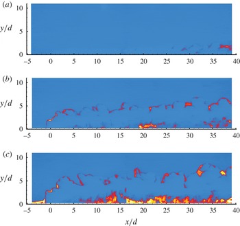
for (a)
 $J=0.3$
, (b)
 $J=2.7$
and (c)
 $J=5.0$
.

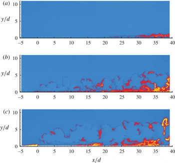
Side-view
 $\text{OH}$
PLIF images on the plane
 $z/d=2$
for (a)
 $J=0.3$
, (b)
 $J=2.7$
and (c)
 $J=5.0$
.

Side-view
 $\text{OH}$
PLIF images on the plane
 $z/d=5$
for (a)
 $J=0.3$
, (b)
 $J=2.7$
and (c)
 $J=5.0$
.

4.1. The reacting shear layer
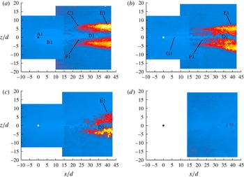
Figure 9 shows an example of the instantaneous reaction zone marked by
 $\text{OH}$
PLIF for the symmetry centreplane
 $(z/d=0)$
of the transverse jet for three
 $J$
cases: (a) the low-value case of
 $J=0.3$
, (b) the intermediate-value case of
 $J=2.7$
and (c) the high-value case of
 $J=5.0$
. These three cases were selected to be representative of the three regimes identified by the
 $\text{OH}^{\ast }$
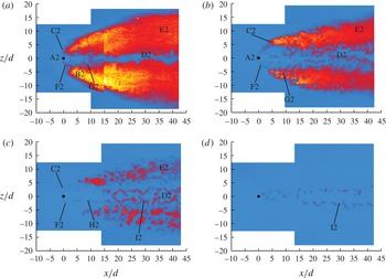
imaging in figure 5. Figures 10 and 11 are the corresponding
 $\text{OH}$
PLIF images for off-centre planes located at
 $z/d=2$
and 5 respectively. We observe that burning in the shear layer becomes stable (within the available field of view) only when
 $J$
is sufficiently large; in our case for
 $J>1$
.
Under the current flow conditions and for sufficiently high values of
 $J$
(here
 $J\sim 5$
, see figure 9
c), three major flow features are observed: (i) an intermittently reacting recirculation region upstream of the jet, (ii) a reactive shear layer on the windward side of the transverse jet (figures 9
c and 10
c) and (iii) a highly reactive boundary layer that extends laterally for several diameters off the jet centreplane (figure 11
c). Figure 11 clearly demonstrates the presence of the reactive boundary layer away from the immediate vicinity of the wake of the jet and that this feature exists for all
 $J$
cases. At low values of
 $J$
(figures 9
a–11
a), the shear layer does not sustain a stable and continuous reaction layer, but the predominant burning region is in the wake near the wall and away from the centreplane. For low
 $J$
, ignition in the shear layer is a relatively weak feature, even on the centreplane of the jet (figure 9
a), and it is not anchored in the near field. The burning upstream recirculation region is also not observed. It seems therefore reasonable to assume that the intense near-wall burning observed from
 $\text{OH}^{\ast }$
chemiluminescence is primarily due to the intense
 $\text{OH}$
regions near the wall. Many of the features observed in the centreplane side views of figure 9 are consistent with previous experimental investigations on similar systems (Lee et al.
Reference Lee, McMillin, Palmer and Hanson1992; Ben-Yakar et al.
Reference Ben-Yakar, Kamel, Morris and Hanson1998). However, contrary to the observations of Ben-Yakar & Hanson (Reference Ben-Yakar and Hanson1998), when ignition occurs upstream or just downstream of the injection point, flame quenching is not observed as the flow expands around the base of the transverse jet.
For the case with the largest value of
 $J$
tested in this study, we observed
 $\text{OH}$
well upstream of the injection point. Specifically, the flame is consistently anchored 5–6 jet diameters upstream of the injection point. This feature is found only at
 $J=5.0$
even if burning in the shear layer is detected.
The
 $\text{OH}$
layers in the shear layers are generally thin (compared with the overall size of the jet, for example); they are convoluted and discontinuous possibly due to local extinction. Most of the layers are organized in bulges that resemble large-scale vortical structures of shear layers. Furthermore, moving away from the centreplane we can observe that the reaction layers merge with regions where
 $\text{OH}$
is distributed in space and that dwell on the wall (figure 10). Connection of the shear layer with the near-wall burning regions, which are relatively stable, might provide a mechanism for shear layer flame stabilization.
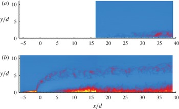
Average side-view
 $\text{OH}$
PLIF image on the centreplane for (a) the
 $J=0.3$
(nine-frame average) and (b) the
 $J=5.0$
(11-frame average) JISCF.

4.2.
 $\text{OH}$
layer thickness

Figure 12 shows average
 $\text{OH}$
PLIF images for the
 $J=0.3$
and
 $J=5.0$
cases. The average was computed over a small number of repetitions (nine for the
 $J=0.3$
case and 11 for the
 $J=5.0$
case). In spite of the fact that the average is clearly not statistically converged, it demonstrates the repeatability of the flow features shown by the set of instantaneous images shown previously. Furthermore, it demonstrates the intermittent nature and corrugation of the reacting shear layer that results in a relatively broad region where the reacting shear layer typically exists. For the low-
 $J$
-value case, what is here referred to as the reacting shear layer can exist anywhere between the wall and
 $3d$
off the wall. For the high-
 $J$
-value case, the reacting shear layer exists in a well-defined band. The thickness of this band is seen to grow from the injection point in the region of maximum deflection, and then to remain nearly unchanged as the jet develops in the wake. In the wake, this band is approximately
 $3d$
wide.
To better quantify the properties of the reacting shear layer, some of its morphological properties have been investigated statistically. This was done by extracting the OH layer thickness, location and orientation from the set of instantaneous images used to construct the average field shown in figure 12. We were able to carry out this analysis only on the
 $J=5.0$
case because we did not have sufficient samples for other (lower-
 $J$
) cases or the reacting shear layer was absent (for the
 $J=0.3$
case). In particular, the
 $\text{OH}$
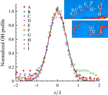
layers in the shear layer were extracted using an algorithm based on the one by Tsurikov (Tsurikov Reference Tsurikov2002; Tsurikov & Clemens Reference Tsurikov and Clemens2002). The algorithm first identifies and classifies the layer, then finds its centreline, thus its direction, and finally defines the layer profile along a line perpendicular to the local direction of the layer. The process is shown in figure 13, where in the inset an
 $\text{OH}$
PLIF image is shown along with the positions of some profiles (labelled A–J), while the main figure shows the (normalized) layer profiles (A–J) plotted as a function of
 $s/{\it\lambda}$
;
 $s$
is the coordinate across the profile and
 ${\it\lambda}$
is the width of the profile, which is defined as the full-width at half-maximum of a Gaussian curve fitted to the profile. The solid line shown in figure 13 indicates a normalized Gaussian demonstrating the similarity between the central portion of the profiles and a Gaussian curve. It should be noted, however, that the resemblance of the profiles to a Gaussian is primarily attributed to spatial resolution limitations (blurring) introduced by the imaging system used. To approximately account for some of these limitations, the image blurring estimation method of Wang & Clemens (Reference Wang and Clemens2004) was used to correct the measured layer thickness
 ${\it\lambda}$
by the blurring introduced by the imaging system (after its point spread function was approximately measured).
Normalized profiles of selected OH layers on the centreplane of the
 $J=5.0$
JISCF.

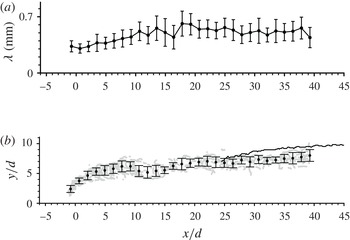
Figure 14 shows the streamwise distribution of (a) the
 $\text{OH}$
layer thickness
 ${\it\lambda}$
and (b) the position. In both figures, the black circles with error bars are average values evaluated over
 $2d$
-wide vertical bands; the error bars are the corresponding root-mean-squared (RMS) values. Furthermore, the grey circles in figure 14(b) show the instantaneous locations of all extracted layers over the 11 frames while the solid black line is the flame boundary defined previously from the
 $\text{OH}^{\ast }$
chemiluminescence images (see figure 4
c). The figures suggest that the
 $\text{OH}$
layer thickness is (on average) approximately 0.3 mm in the near field and rapidly grows to approximately 0.5 mm. The thickness then remains fairly constant in the wake of the JISCF.
(a) Streamwise distribution of
 $\text{OH}$
layer thickness, with error bars indicating its RMS value. (b) Penetration of
 $\text{OH}$
layers. Both figures refer to
 $J=5.0$
JISCF measurements on the centreplane. In (b) ●, mean location of the
 $\text{OH}$
layer with error bars indicating its RMS value; ○, instantaneous location of the
 $\text{OH}$
layer extracted from the set of instantaneous
 $\text{OH}$
PLIF images; the black solid line indicates the flame boundary extracted from the
 $\text{OH}^{\ast }$
imaging results (figure 4
c).

Because the
 $\text{OH}$
regions are organized in layer-like structures, one can approximate their description as strained laminar diffusion layers (Buch & Dahm Reference Buch and Dahm1996, Reference Buch and Dahm1998; Kothnur & Clemens Reference Kothnur and Clemens2005). In this respect, the
 $\text{OH}$
layers can thus be thought of as marking flamelets where combustion occurs, and their modelling can follow the flamelet model (Peters Reference Peters1984; Pitsch, Chen & Peters Reference Pitsch, Chen and Peters1998). For a constant-density steady formulation, the characteristic thickness
 ${\it\lambda}$
of a strained laminar (non-reacting) diffusion layer can be written as
 $$\begin{eqnarray}{\it\lambda}\sim \sqrt{\frac{\mathscr{D}}{S}},\end{eqnarray}$$
where
 $S$
is a characteristic (local) strain rate and
 $\mathscr{D}$
is a scalar diffusivity. Assuming that
 $\mathscr{D}$
does not vary spatially along the shear layer of the transverse jet, the layer thickness only inversely depends on the strain rate. We can approximate the strain rate as the ratio between a characteristic local velocity scale and the length scale of the transverse jet. From the (incompressible) scaling law results of Hasselbrink & Mungal (Reference Hasselbrink and Mungal2001), we can take the local centreline-to-free stream velocity difference and jet penetration as suitable scale quantities in the limit that compressibility does not play a role. Thus, for both the near and far fields, we can readily derive that the expected dependence of
 ${\it\lambda}$
on
 $x/d$
is
 ${\it\lambda}\sim (x/d)^{1/2}$
. By this result, we would expect that
 ${\it\lambda}$
continuously increases with the downstream distance
 $x/d$
. An increase of
 ${\it\lambda}$
with
 $x/d$
is qualitatively observed only for the near field and the region of maximum deflection (figure 14
a); on the contrary,
 ${\it\lambda}$
remains nearly constant for downstream distances larger than
 $x/d\approx 20$
. If the approximation of the
 $\text{OH}$
layers as strained diffusion layers is correct and if their dependence on
 $S^{-1/2}$
is accepted, then a constant
 ${\it\lambda}$
for
 $x/d>20$
indicates that the large-scale strain rate in the far field remains unchanged. This would require that both the characteristic velocity and length scales remain constant or vary at the same rate with
 $x/d$
.
Figure 14(b) shows the instantaneous and ensemble-averaged positions of the
 $\text{OH}$
layers. We define this quantity as the
 $\text{OH}$
flame boundary or penetration. Their mean position is equivalent to the
 $\text{OH}^{\ast }$
flame boundary we defined previously. The
 $\text{OH}$
and
 $\text{OH}^{\ast }$
flame boundaries are thus compared in the figure (the solid line is the
 $\text{OH}^{\ast }$
boundary). As one would expect, the
 $\text{OH}^{\ast }$
flame boundary is found to capture the outer envelope of where the instantaneous
 $\text{OH}$
layers exist. The error bars in figure 14(b) provide a quantitative measure of the spread of the
 $\text{OH}$
layer locations around the mean value; the spread is in fact a significant fraction (approximately
 $1/4$
th) of the local penetration. It is interesting to note that unlike the subsonic transverse jet, the trajectory defined by the
 $\text{OH}$
boundary is not monotonic. In fact, the trajectory is strongly curved close to the injection point, it contracts around
 $x/d\approx 17$
(as if the jet would ‘neck’), and then steadily increases in the wake. The same contraction in the transverse jet penetration can be recognized in the corresponding Schlieren image of figure 3(b) (near label F). From a comparison with the Schlieren images, this feature seems to be associated with the presence of the recompression shock (label E in figure 3
b) formed on the lee side as the flow expands around the base of the jet. A similar non-monotonic near-field penetration was also observed in the trajectories extracted from the mixing studies of Rogers (Reference Rogers1971b
) (see also Povinelli & Povinelli Reference Povinelli and Povinelli1971); they observed a contraction of the penetration in the region
 $7<x/d<20$
. It should also be pointed out that a
 $J=5$
transverse jet is one with a relatively low value of the momentum flux ratio (in the context of transverse jets); thus, a near field with a well-developed jet-like behaviour is not expected (Smith & Mungal Reference Smith and Mungal1998; Hasselbrink & Mungal Reference Hasselbrink and Mungal2001). Furthermore, in the supersonic case there exists also a (distorted) barrel shock that might affect the evolution of the transverse jet in the portion of maximum deflection. The combination of these two effects could also be responsible for or at least participate in the formation of the contraction (necking) observed at
 $x/d\approx 17$
. Because we cannot extend the same analysis to all other cases, we cannot conclude that the necking in the OH flame boundary is a universal feature (i.e. that it exists for the lower-
 $J$
cases). However, we note that Rogers (Reference Rogers1971b
) observed a similar feature in his non-reacting experiments for
 $J$
from 0.5 to 1.5. Finally, it is interesting to note that the point of necking of the OH flame boundary in figure 14(b) corresponds to a local minimum in the OH layer thickness in figure 14(a) at
 $x/d\approx 16$
. If the necking is associated with the recompression shock, it is also possible that the recompression shock acts to further strain the OH layers, thus decreasing their thickness locally.
To further quantify the properties of the
 $\text{OH}$
layers, probability density functions (PDFs) of the layer width
 ${\it\lambda}$
and orientation
 ${\it\theta}$
(with
 $0\leqslant |{\it\theta}|\leqslant {\rm\pi}/2$
) were computed at different downstream bands. The layer orientation
 ${\it\theta}$
is defined as the magnitude of the angle between the layer and the
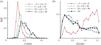
 $x$
-axis. The resulting PDFs are shown in figure 15. Figure 15(a) shows PDFs of the thickness
 ${\it\lambda}$
evaluated in a region around the injector (
 $|x/d|<5$
) and in selected downstream regions. At the injector, the distribution of
 ${\it\lambda}$
is relatively narrow with a peak value near 0.3 mm. At the first band downstream of the injector (
 $5\leqslant x/d\leqslant 10$
), the PDF shifts to larger values and begins to broaden with a long tail at large values of
 ${\it\lambda}$
. Then, the distribution for
 $x/d>10$
remains the same at all other downstream regions; it is relatively broad with a peak value near 0.5 mm. It is also interesting to note that in all regions the PDFs show a sharp edge on the low-
 ${\it\lambda}$
-value side, while a longer tail on the high-value side. In general, values of less than approximately 0.2 mm (a value that could be limited by the imaging set-up) or larger than approximately 1 mm (a value that could be limited by our layer detection definition and algorithm) are never detected.
Figure 15(b) shows the corresponding PDFs for the
 $\text{OH}$
layer orientation angle
 ${\it\theta}$
, where only its magnitude is reported. This was necessary to obtain smoother PDFs due to the overall limited number of samples. For the same reason, only three downstream bands were considered. The figure shows that at the injection point there is a strong tendency of the
 $\text{OH}$
layer to be nearly vertical (
 ${\it\theta}={\rm\pi}/2$
). Furthermore, it is overall more likely to observe an orientation angle larger than
 ${\rm\pi}/4$
. On the contrary, downstream of the injection point, the
 $\text{OH}$
layers are more likely to be oriented parallel to the free stream,
 ${\it\theta}=0$
, or in any case, at an angle of less than
 ${\rm\pi}/4$
. Thus, throughout the evolution of the windward side of the shear layer of the transverse jet, the
 $\text{OH}$
layers tend to track the interface between the jet and crossflow streams. Furthermore, the fact that the layer orientation is mostly parallel to the free stream in the wake indicates that the shear (i.e. velocity difference) between the wake and the crossflow is small, or at least insufficient to generate large-scale rollers that can promote entrainment and thus rapid mixing and combustion. In this respect, chemical reaction along the wake of the jet progresses in a purely diffusion-dominated fashion with minimal enhancement by large-scale turbulent structures. Thus, overall, the wake of an isolated JISCF cannot be regarded as an efficient system for supersonic combustion (at least for hydrogen/air combustion) consistent with wake-like behaviour.
The PDF of (a)
 $\text{OH}$
layer thickness
 ${\it\lambda}$
and (b) angular orientation
 $|{\it\theta}|$
.

4.3. Near-wall burning
A particular feature of interest is the distribution of
 $\text{OH}$
within the boundary layer near the surface, as was shown by figure 11(a–c). To investigate this flow feature in more detail, plan-view
 $\text{OH}$
PLIF imaging at different wall-normal locations was carried out. Examples at selected wall-normal locations (
 $y/d=0.25$
, 0.5, 1 and
 ${\geqslant}2$
) are shown in figures 16–18 for the
 $J=0.3$
, 2.7 and 5.0 cases respectively. Based on the estimate of the boundary-layer thickness at the injection point given previously and from the side-view
 $\text{OH}$
images, the measurement plane at
 $y/d=0.25$
is well within the (undisturbed) boundary layer, while that at
 $y/d=0.5$
is approximately at the edge of it. Thus, for each figure, panels (a–c) identify the structure of the
 $\text{OH}$
regions within the boundary layer, while panel (d) identifies the structure somewhere in the shear layer. It should be noted that the flow features in these figures have been labelled with an alphabetical letter followed by a number (e.g. C1), such that the letter indicates corresponding flow features across different
 $J$
cases while the number identifies the three cases reported in the set of figures. It should be noted that labels used in figures 16–18 do not necessary correspond to the same labels and flow features as indicated in figure 4. The main flow and combustion features identified in figures 16–18 are also summarized in table 3.
 $\text{OH}$
PLIF imaging on selected plan-view planes for the
 $J=0.3$
JISCF. Plan views at (a)
 $y/d=0.25$
, (b)
 $y/d=0.5$
, (c)
 $y/d=1$
and (d)
 $y/d=2$
.

 $\text{OH}$
PLIF imaging on selected plan-view planes for the
 $J=2.7$
JISCF. Plan views at (a)
 $y/d=0.25$
, (b)
 $y/d=0.5$
, (c)
 $y/d=1.0$
and (d)
 $y/d=3.0$
.


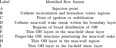
Cases corresponding to
 $J$
values lower than approximately 3 are characterized by a plan-view imprint of the reaction zone that is consistently similar to the case of figure 16 (
 $J=0.3$
). They are characterized by (i) long separation between the injection hole (A1 in figure 16) and the point of ignition (C1 in figure 16), and which is consistent with the stabilization point measurements of figure 5 extracted from the time-averaged
 $\text{OH}^{\ast }$
imaging; (ii) a broad region where a diffuse distribution of
 $\text{OH}$
exists (E1 in figure 16); this region is several jet diameters wide and grows with downstream distance; (iii) a characteristic spreading of the
 $\text{OH}$
regions E1 downstream of the ignition point C1 that consistently grows with
 $J$
(compare the cases of figures 16 and 17); (iv) a narrow wandering region or streak (of the order of two jet diameters in size) located along the symmetry plane where burning does not occur (region D1 in figure 16); this non-reacting streak in the wake of the JISCF also exists for larger
 $J$
, as indicated by regions D2 and D3 in figures 17 and 18; (v) the thickness (from the plate surface) of the region of diffuse
 $\text{OH}$
is at most of the order of one jet diameter since measurements on planes above
 $y/d=1$
only show the reacting shear layer of the transverse jet. The thickness of the
 $\text{OH}$
region at the wall remains nearly the same for all cases, with a small initial growth with downstream distance. This was also better shown by the side-view
 $\text{OH}$
images, and it is in agreement with the thickness of the intense
 $\text{OH}^{\ast }$
layer that was observed near the plate surface from figure 4. In agreement with the results of figure 5, the point of stabilization (C1 in figure 16) moves upstream and reaches the injector for
 $J\approx 3$
; see point C2 on the
 $y/d=0.25$
plane for the
 $J=2.7$
case (figure 17). For larger
 $J$
, the stabilization point moves upstream of the injection point; see point C3 on the
 $y/d=0.25$
plane for the
 $J=5.0$
case (figure 18).
 $\text{OH}$
PLIF imaging on selected plan-view planes for the
 $J=5.0$
JISCF. Plan views at (a)
 $y/d=0.25$
, (b)
 $y/d=0.5$
, (c)
 $y/d=1.0$
and (d)
 $y/d=3.0$
.

The relative spanwise size of these burning regions increases with
 $J$
. The broad diffuse
 $\text{OH}$
regions at the wall (
 $y/d=0.25$
) for
 $J=0.3$
(figure 16) are of the order of
 $\pm 5d$
wide, and they grow to
 $\pm 15d$
for
 $J=2.7$
by the end of the measurement domain (
 $x/d=40$
). The spanwise extent increases further to more than
 $\pm 20d$
for the
 $J=5.0$
case. Furthermore, these regions grow laterally with an apparent origin that approximately corresponds to the injector.
The morphological characteristics of the near-wall
 $\text{OH}$
layer begin to significantly change for the
 $J=5.0$
case where some drastic modification takes place. The main difference for the
 $J=5.0$
case is that stabilization appears upstream of the injection point – see C3 in figure 18(a) – along with the existence of a significantly large
 $\text{OH}$
footprint near the wall. We will discuss this further below, but it is believed that the flow structure that leads to the
 $\text{OH}$
imprint of figure 18 is related to the strength of the bow shock and the importance of shock/boundary-layer interaction on the near-field flow and mixing characteristics (Gamba et al.
Reference Gamba, Terrapon, Saghafian, Mungal and Pitsch2011).
Comparison of the
 $\text{OH}$
imaging results for the different cases on side and planviews (including additional side- and plan-view measurement planes available but not shown here), suggests that the thickness of the near-wall
 $\text{OH}$
regions is relatively independent of the value of
 $J$
, or at most a very weak function of it. In fact, in all cases the edge of these burning regions is located at approximately
 $y/d=1$
. We therefore conclude that one of the controlling flow parameters in determining the properties of this reacting region is the incoming boundary-layer thickness. More specifically, we speculate that this feature is primary related to the structure and properties of the incoming boundary layer (recall that the boundary layer is laminar and approximately
 $0.5d$
thick in this study) and its tendency to separate upon interaction with the bow shock. Therefore, we believe that the observed near-wall imprint is an extensive reacting boundary layer where fuel entrainment is sustained by the upstream recirculation region (which for sufficiently large values of
 $J$
also serves as a point of flame stabilization) and by the bow shock/jet interaction.
Imaging several diameters off the plate surface detects only the reacting shear layer of the jet (see figures 17
d–18
d). Because of the small penetration of the
 $J=0.3$
case and the weak tendency of the shear layer to react, a well-defined reacting shear layer is not found in this case. The reacting shear layer on
 $y/d=3$
(
 $J=2.7$
and 5.0) shows characteristics similar to the
 $\text{OH}$
side views shown previously; it is in fact part of the shear layer system of the main body of the transverse jet. The lateral extent of the jet body is significantly narrower than what is observed near the plate, being only a few diameters wide (at most
 $\pm 7d$
for the
 $J=5.0$
cases, for example). By combining information about the location of the reacting
 $\text{OH}$
layers from side and plan views we can also infer that the cross-section (i.e. on a
 $y$
–
 $z$
plane) shape of the reacting shear layer has nearly a 1:1 aspect ratio.
Similarly to low-speed transverse jets, the wake of the jet is dominated by a CVP (e.g. Santiago & Dutton Reference Santiago and Dutton1997; Smith & Mungal Reference Smith and Mungal1998) generated during the jet deflection process by reorganization of vorticity. The CVP has a significant role in crossflow entrainment and mixing in the wake of the jet (VanLerberghe et al.
Reference VanLerberghe, Santiago, Dutton and Lucht2000). For low
 $J$
, the penetration of the jet is only a few jet diameters deep and the evolution of the CVP is inevitably constrained by the presence of the wall. The strength of the interaction of the CVP with the wall and the boundary layer would be expected to increase with diminishing jet penetration (i.e.
 $J$
). However, even the highest-
 $J$
-value case considered here remains a case with an overall low value of
 $J$
if compared with many of the transverse jets studied within the low-speed regime. Therefore, the observed near-wall structure of the
 $\text{OH}$
regions is also a result of the constrained evolution of the CVP interaction with the near-wall flow.
Generally speaking, the
 $\text{OH}$
distribution near the wall for
 $y/d<1$
occurs over broad contiguous regions in space. For
 $J<3$
there are two main contiguous regions about the streamwise plane of symmetry of the system where most of the
 $\text{OH}$
is found. Although it is difficult to establish solely from these results, this observation suggests that the combustion process near the wall might progress either as a premixed/partially premixed mode, or a non-premixed distributed reaction zone mode. We will return to this below. A closer inspection of the
 $\text{OH}$
fields reveals that thin
 $\text{OH}$
layers are also present at the inner interface of the jet wake. This might indicate that the combustion process in the near-field near-wall region might proceed in a complex fashion characterized by different but coexisting combustion modes (regimes). Examples of thin
 $\text{OH}$
layers are indicated by labels F1 for the
 $J=0.3$
case, F2, H2 and I2 for the
 $J=2.7$
case, and F3, H3 and I3 for the
 $J=5.0$
case. The thin
 $\text{OH}$
layers are embedded and at times connected to the regions where
 $\text{OH}$
is broadly distributed in space and appear to be primarily associated with regions in the immediate wake of the transverse jet. For the
 $J=0.3$
case, features F1 and C1/E1 (see figure 17
a,b) define a two-region (or regime) burning feature: F1 is associated with localized thin reaction at the boundary between the (fuel-rich) wake and the outer flow (effectively this is the shear layer of the transverse jet), while E1 is the region where
 $\text{OH}$
occurs broadly. For the
 $J=2.7$
and 5 cases, the thin
 $\text{OH}$
layers exist throughout the jet. For example, thin layers are found to wrap around the injector (features F2 and F3), and to extend in the wake (H2/I2 and H3/I3) mixed with regions where
 $\text{OH}$
occurs broadly.
The set of plan-view
 $\text{OH}$
images indicates that ignition in the recirculation region in front of the transverse jet occurs only at large
 $J$
(in this case only for
 $J=5.0$
) with a characteristic bow shape, while broadly distributed
 $\text{OH}$
is visible downstream of the injector for most of the
 $J$
cases. As shown in figure 18(a,b), this reacting recirculation region wraps around the base of the jet with a characteristic ‘hole’ just in front of the injector. Very close to the wall (
 $y/d=0.25$
, see figure 18
a), the
 $\text{OH}$
is distributed uniformly and no structure is observed; on the contrary, at higher locations (
 $y/d=0.5$
, see figure 18
b) the
 $\text{OH}$
is organized in stretched loops (see B3) connected to the
 $\text{OH}$
layers of the windward shear layer (F3) mixed with regions characterized by
 $\text{OH}$
streaks originating at a virtual point (for example C3 in figure 18
b). The analysis of Huber et al. (Reference Huber, Schexnayder and McClinton1979) on ignition and flame-holding capabilities of different wall-injection configurations identified the upstream recirculation as a suitable location for flame stabilization due to the long residence time and near-stagnation conditions. Therefore, the length of the upstream recirculation region (which increases with
 $J$
) (Dowdy & Newton Reference Dowdy and Newton1963), the low velocities associated with it (Santiago & Dutton Reference Santiago and Dutton1997) and the blockage effect of the jet (which increases with
 $J$
) would play an important role in this process. Another mechanism supporting ignition in the separation region is the favourable mixing that occurs as a result of the interaction of the issuing jet and the system of recirculation regions (Thayer Reference Thayer1971; Yoshida & Tsuji Reference Yoshida and Tsuji1977; Huber et al.
Reference Huber, Schexnayder and McClinton1979) along with the shorter ignition times expected at lean conditions in supersonic non-premixed combustion of a cold fuel mixed with a hot oxidizer (Huber et al.
Reference Huber, Schexnayder and McClinton1979) that could be observed in the upstream recirculation region.
The burning structure in the upstream recirculation region and around the base of the jet is not observed at
 $J$
values lower than 5. However, for the other
 $J$
cases, a structure that resembles a horseshoe vortex system can still be recognized by tracking regions of low background signal. In fact, it was found that the free stream generated a detectable level of background signal in the images. The origin of this background is not fully understood, but it is observed in high-temperature free streams (the background is not present for testing conditions at lower free stream temperatures) and not in regions where pure fuel exists. Therefore, although this background is unwanted, it provides a convenient marker of free stream fluid and it can serve to identify regions rich in injectant, especially in the near field and in the recirculation region of the jet. An example of this effect is indicated in features A1, B1 and G1 in figure 16(a). Close inspection of the imaging results consistently shows a fuel-rich region that wraps around the injector. By this method, the upstream recirculation region and its size (for example its length) can be identified at all values of
 $J$
. The extent of this region was found to increase with
 $J$
, as also shown in non-reacting transverse jets (Dowdy & Newton Reference Dowdy and Newton1963).
Everett et al. (Reference Everett, Woodmansee, Dutton and Morris1998) carried out surface oil-flow visualization around transverse jets (at
 $J=1{-}2$
) to investigate the streamline pattern resulting from the interaction of the jet with the bow shock and the boundary layer. They identified two separation lines that wrap around the jet and that create two separate non-interacting regions. Between these two separation lines, and between the second separation line and the injector, two recirculation bubbles exist. The first recirculation region is associated with the boundary layer, whereas the second recirculation region is produced by the issuing jet (see also figure 1 for a schematic diagram). Everett et al. observed that oil used to mark the wall streamline did not move across these two recirculation systems. However, from the imaging of the current study, it is clear that transfer across the two recirculation regions has to occur to provide fuel to sustain combustion within the large interaction region. We thus believe that the ‘hole’ visible in the reacting upstream region is associated with the second recirculation region (which is fuel-rich), while the reacting portion (further upstream of the ‘hole’) is the first recirculation region where reaction can occur. The oil-flow visualization of Everett et al. also showed that streamlines at the wall follow the trajectory of the separation streamlines and they all wrap around the base of the jet. Furthermore, they also identified a third recirculation region just downstream of the injector which did not interact with the upstream separation lines. This third recirculation region originates at the injector and extends to a triangular region downstream of the injector that is then swept downstream in the wake of the jet. This third recirculation region defines a fuel-rich region that might not experience sufficient free stream entrainment; thus, it could be the origin of the unburned region developing in the wake of the jet (D3).
Many of the features observed by the oil-flow visualization experiments of Everett et al. (Reference Everett, Woodmansee, Dutton and Morris1998) share many similarities with the flow structures marked by
 $\text{OH}$
shown in figure 18(a) for the
 $J=5$
case. For example, the broad
 $\text{OH}$
regions that wrap around the jet show finger-like structures (G2 and G3 for example) in the wake of the jet that close towards the jet centreplane in a fashion that is reminiscent of the streamlines shown by Everett et al. The main difference between the case shown here and the case described by Everett et al. is that the upstream recirculation region observed in the current work does wrap around the base of the jet, but does not close behind it as they observed instead.
One last feature of interest is the unburnt streak that develops from the injection point into the wake near the wall (feature D in figures 16–18). This region exists for all
 $J$
cases considered, and it is very clear as the wall is approached (i.e. at
 $x/d=0.25$
). For the
 $J=0.3$
case (D1 in figure 16), this streak is well defined in the wake and it is bounded by broadly diffused
 $\text{OH}$
regions. For the higher-
 $J$
-value cases (see D2 and D3 in figures 17 and 18 respectively), the streak remains an isolated feature very close to the wall (
 $x/d=0.25$
), but it becomes less distinct from the other regions as the measurement plane is farther away from the plate. Nevertheless, its signature can still be identified. Furthermore, at higher planes, the streak becomes more convoluted by the reacting regions bounding them and is confined by thin layered
 $\text{OH}$
regions (I2 and I3 respectively) instead of the broader
 $\text{OH}$
regions at the lowest plane. It appears that this unburnt region might be part of, or connected to, the fuel-rich wake of the transverse jet. In particular, it might be the part of the far-field wake of the jet that interacts with the wall, limiting entrainment of oxidizer, and thus preventing combustion. At low
 $J$
, the wake remains within the boundary layer and its evolution is strongly limited by the wall. For the higher-
 $J$
cases, the wake penetrates away from the boundary layer, so it can freely develop. Therefore, there can be regions characterized by thin reaction layers away from the wall (features I2 and I3 for example), which merge with the regions of broad distributions of
 $\text{OH}$
as the wall is approached.
5. Discussion
The results of the previous sections demonstrated the strong dependence of many of the flow features of transverse jets on
 $J$
. Ignition and flame stabilization also appear to be strongly affected by this single parameter. Near-field ignition characteristics are particularly affected by it. The value of
 $J$
dictates the penetration of the jet which drives the blockage effect and induces the three-dimensional bow shock around the jet. Interaction of the bow shock with the jet and the boundary layer triggers the system of upstream recirculation regions. All of these processes are closely coupled and they all affect entrainment, mixing and flame stability. The resulting complex systems of recirculation regions seem to especially control the mixing and stability processes. Furthermore, the dynamics of the shock system is closely coupled to the dynamics of the underlying turbulent flow, which in turn is responsible for the mixing between jet and crossflow fluid. This coupling has been clearly shown by the work of Kawai & Lele (Reference Kawai and Lele2010). On the contrary, the local properties in the wake of the jet are less affected by
 $J$
. Finally, the incoming boundary layer and how it responds to the shock system plays a key role in the mixing (Kawai & Lele Reference Kawai and Lele2010) and stabilization processes.
Generally speaking, the flame stabilizes at two different regions based on the value of
 $J$
: in the boundary layer in the wake of the transverse jet for low
 $J$
or in the near-field recirculation regions for large
 $J$
. Stabilization at both locations was observed at intermediate
 $J$
.
For low
 $J$
(
 ${\leqslant}1$
), the flame is similar to a lifted flame. Different mechanisms are believed to contribute to the stabilization process in lifted flames (Lyons Reference Lyons2007; Lawn Reference Lawn2009). We speculate that in this case stabilization in the wake can be reduced to an autoignition process. For hydrogen/air chemistry, the ignition delay time
 $t_{ig}$
is limited by the
 $\text{H}/\text{O}_{2}$
chain branching reaction and, thus, it is correlated with temperature and pressure as
 $t_{ig}p\sim \text{e}^{{\it\Theta}/T}$
(in the context of supersonic combustion, see for example Huber et al.
Reference Huber, Schexnayder and McClinton1979; Mitani, Chinzei & Kanda Reference Mitani, Chinzei and Kanda2001), where
 ${\it\Theta}$
is a suitable characteristic temperature. Pressure and temperature should be interpreted as suitable local values; for example, the temperature could be interpreted as the flow recovery temperature (Mitani et al.
Reference Mitani, Chinzei and Kanda2001). The pressure distribution in the near field of the jet is highly non-uniform. Peak values of pressure depend on the value of
 $J$
(Everett et al.
Reference Everett, Woodmansee, Dutton and Morris1998; Gruber & Goss Reference Gruber and Goss1999) and they can be several times the free stream pressure within the upstream separation region for large
 $J$
and much less in the leeward side of the near field. Further downstream, the pressure recovers to the free stream value. Temperature may vary in a similar fashion. Thus, the time-integrated histories of temperature and pressure could also affect the process. Comparison of
 $t_{ig}$
with a characteristic time of the flow determines whether and where local ignition might occur.
To this end, we have calculated the ignition delay times for hydrogen/air mixtures using the hydrogen mechanism of Hong, Davidson & Hanson (Reference Hong, Davidson and Hanson2011) for different equivalence ratios
 ${\it\phi}$
of the mixture. To replicate the mixing process occurring under the conditions of this study, we assume isobaric mixing of 1400 K air with 300 K hydrogen in a given ratio (i.e.
 ${\it\phi}$
), followed by ignition. It should be noted that by this model, the temperature of the unburned mixture varies with the equivalence ratio – thus it will affect the ignition delay time. In practice, we have reconstructed the model of Huber et al. (Reference Huber, Schexnayder and McClinton1979) with an updated chemical mechanism and conditions specific to our study. The results at three different pressures are shown in figure 19. The values of pressure selected here correspond to the free stream value (
 $p_{a}=40~\text{kPa}$
), and characteristic lower and upper values (2.5 and 4 times
 $p_{a}$
for
 $J\sim 1$
and
 $J\sim 4$
respectively) that are expected in the upstream recirculation region for our range of
 $J$
(estimated from measurements of similar cases, e.g. Everett et al.
Reference Everett, Woodmansee, Dutton and Morris1998; Gruber & Goss Reference Gruber and Goss1999). The oxidizer temperature was approximated with the free stream value. However, for regions within the boundary layer, this approximation needs some explanation. First of all, our experiments were conducted in a high-temperature environment, but the temperature of the flat plate remained close to the initial value (room temperature) because of the short test times of the experiments (in fact, all hardware remained near room temperature). This was verified by conducting wall temperature measurements at selected locations along the expansion tube (but not on the flat plate itself) where a temperature increase of less than 10 K over the duration of the test was found. Furthermore, it was found that this change in wall temperature was associated with large values of heat fluxes to the wall even if the flow evolved in short times. The boundary layer is a compressible (Mach 2.4) boundary layer with a constant low-temperature wall. Because of the relatively low Mach number, viscous heating within the boundary layer is, however, expected to be small. Thus, the maximum temperature found in the boundary layer is expected to be close to the free stream value and not near the recovery value. This is approximately true for a laminar low-Mach-number supersonic boundary layer over a cold wall (White Reference White1991). Therefore, recovery temperature effects are not believed to be significant in our configuration unless strong stagnation regions occur in the flow field, as for example in the upstream recirculation region for large values of
 $J$
.
Ignition delay time
 $t_{ig}$
as a function of the equivalence ratio
 ${\it\phi}$
for isobaric mixing of 1400 K air with 300 K hydrogen. The ignition point
 $x_{ig}$
is approximated simply as
 $x_{ig}=1/2U_{a}t_{ig}$
.

Figure 19 shows the ignition delay time
 $t_{ig}$
as a function of
 ${\it\phi}$
. For comparison,
 $t_{ig}$
is also converted to an equivalent ignition point
 $x_{ig}$
by assuming a convective velocity within the boundary layer equal to half the free stream value. This is just a coarse approximation of a more complex convection process within the boundary layer and the wake of the transverse jet. The ignition point is equivalent to the stabilization point
 $x_{s}$
defined in figure 5. The results of figure 19 show that there is a relatively strong nonlinear and non-monotonic dependence of the ignition delay on the mixing process (i.e. on
 ${\it\phi}$
). Ignition within a reasonably short length (say, within
 $50d$
) can occur only for a well-defined and relatively limited range of
 ${\it\phi}$
values: too little (too lean) or too much (too rich) mixing may just result in flame blow-off. This suggests that there might be a strong sensitivity of stabilization by autoignition to mixing.
The condition of minimum ignition delay time is found to be at approximately
 ${\it\phi}=0.25$
, i.e. for very lean mixtures, and not near
 ${\it\phi}=1$
as one might expect. This is a result of competing effects on the ignition delay due to non-isothermal mixing (
 ${\it\phi}$
) and temperature effects on the chemistry. It is a consequence of the fact that the ignition delay time increases with
 ${\it\phi}\rightarrow 0$
(and
 ${\it\phi}\rightarrow \infty$
), but decreases with increasing temperature (and pressure). In the model constructed here, as
 ${\it\phi}$
is varied from
 ${\it\phi}=0$
to
 ${\it\phi}\rightarrow \infty$
, the temperature of the unburnt mixture varies from the oxidizer value (high temperature) to the fuel value (low temperature). Thus, lean mixtures have higher temperatures than stoichiometric ones. The overall effect results in shorter ignition delay times at (fuel) lean mixtures. Minimum
 $t_{ig}$
at lean
 ${\it\phi}$
values implies that limited mixing of fuel into the crossflow has to occur to generate a rapidly ignitable mixture. The effect of (increasing) pressure is to lower
 $t_{ig}$
for slightly leaner mixtures. A case at higher pressure corresponds to a case with larger
 $J$
where pressure time-history effects in the near field might be present. If the initial oxidizer temperature is increased,
 $t_{ig}$
decreases significantly, but the general trend remains the same (not shown). The case of higher oxidizer temperature also corresponds to a case with larger
 $J$
because of stagnation in the upstream recirculation region or the presence of a stronger bow shock. Comparison of the measured point of stabilization (figure 5) with the approximation of figure 19 is very poor, but the approximations made have to be kept in mind. From figure 5 we observe that
 $x_{s}/d$
is approximately 20 with a weak dependence on
 $J$
until
 $J=1$
(region I in figure 5). The estimated values are much larger than what is observed for a background pressure equal to
 $p_{a}$
. The comparison improves if results at higher pressure are considered. Because of the fairly significant dependence of the ignition delay on quantities associated with the near-field processes, we conclude that the dynamics in this region maintains a dominant role in flame stabilization even in the lifted cases (low
 $J$
).
The near-wall burning zones (at
 $y/d=0.25$
) are characterized by regions where
 $\text{OH}$
occurs broadly after a relatively long lift-off that supports premixing. The observed structure resembles the broad reaction zone of premixed or partially premixed flames rather than the thin and localized reaction zones of non-premixed combustion, as are found in the reacting shear layer of the jet. It should be noted, however, that the presence of regions where
 $\text{OH}$
is distributed broadly could also be a consequence of the slow three-body recombination of
 $\text{OH}$
and fast convective time (Barlow et al.
Reference Barlow, Dibble, Chen and Lucht1990). Nevertheless, the observed structure of the
 $\text{OH}$
regions supports our speculation that the stabilization is autoignition-supported. However, a similar distribution of
 $\text{OH}$
is also observed for high-
 $J$
cases where the flame stabilizes in the upstream recirculation region. Finally, cases of low jet penetration confine fuel near the wall and within the boundary layer only. Therefore, the ratio of the jet penetration to the boundary-layer thickness should be an important parameter for the stabilization process.
For the cases at large values of
 $J$
(
 ${\geqslant}3$
), combustion occurs in two distinct locations: near the wall where
 $\text{OH}$
remains organized in broadly distributed regions and marks the complex flow structure of the transverse jet, and in the shear layer with a flame structure similar to that of a thin reaction layer. Following the previous discussion, we further speculate that the primary stabilization mechanism at large values of
 $J$
(
 ${\geqslant}3$
) is associated with ignition due to shock heating and long residence times at the front of the bow shock and within the upstream separation region. In this case, large values of pressure and temperature exist in the near field because of strong bow shocks, and large recirculation (separation) regions are induced as a consequence (Dowdy & Newton Reference Dowdy and Newton1963). They allow for very low
 $t_{ig}$
compared with a time scale associated with the residence in the separation region. Thus, the flame can stabilize directly in the upstream separation region and in the shear layer behind the bow shock.
Figure 20 schematically summarizes the different fluid dynamic processes that are important for the stabilization and the formation of the overall structure of reacting transverse jets. The schematic diagram shows the 3D structure of the transverse jet of figure 1 with superimposed notional streamlines (labelled A–E) to indicate the different possible paths for entrainment of fuel into the transverse jet. A case for large
 $J$
is considered in constructing the schematic. Some of the entrainment paths discussed here are well captured by the analysis of Kawai & Lele (Reference Kawai and Lele2010), which is used to formulate the various path identified here. In particular, we identify the following.
Three-dimensional schematic diagram of JISCF showing the main fuel entrainment pathways.

-
(i) Path S: fuel ejected goes through the barrel shock system, develops into the windward shear layer, entrains and mixes with crossflow air to form the thin reaction layer (where the term thin is used to indicate that the
$\text{OH}$
layer is thinner than the characteristic size of the shear layer). This path is responsible for the formation of the strained diffusion reacting layers identified in the shear layer by the
$\text{OH}$
PLIF imaging. Flame stabilization in this path occurs only for sufficiently large
$J$
. The occurrence of combustion along this path is believed to be linked to the blockage effects induced at large
$J$
. -
(ii) Path W: part of the fuel ejected through the barrel shock emerges into the lee side of the jet and streams close to the wall in the wake of the injector in a region in between the horseshoe vortex. Fuel is continuously delivered to this region. Combustion does not occur in this region (throughout the range of
$J$
values). This is possibly the result of the region being too cold and fuel-rich so that ignition cannot take place. -
(iii) Path Z: fuel following path W can be transferred by turbulent transport to the horseshoe vortex system that wraps around the base of the transverse jet. The horseshoe vortex originates from the boundary layer, therefore an ignitable mixture can be formed in this region. This path may be one of the two possible paths responsible for the formation of the burning regions observed at low
$J$
near the wall. -
(iv) Path H: fuel leaving the injector is transferred to the upstream separation bubble through the system of recirculation regions. This transfer process is intermittent, highly unsteady and depends on the dynamics of the jet itself. Fuel entrained in the separation bubble may have a residence time sufficient for ignition, thus it is responsible for the formation of the reacting upstream separation region seen at high-
$J$
cases. Furthermore, fuel entrained in the upstream separation region can later be transported into the horseshoe vortex system that develops downstream. Along with path Z, this may be the second, and possibly the dominant, mechanism responsible for the formation of the distributed reacting regions observed at low and intermediate
$J$
values within the boundary layer. In other words, these reacting regions (E1, E2 and E3 in the
$\text{OH}$
PLIF plan views) might be a signature of the horseshoe vortex system. -
(v) Path U: this is another path evolving in parallel to path H. The upstream separation bubble is a three-dimensional structure that wraps around the jet following the bow shock. Thus, fuel entrained in the upstream separation bubble can be transferred into the region of separated flow under the bow shock and then ultimately washed downstream in the boundary layer. This path is relevant only for high
$J$
(here
$J=5.0$
) because it requires a strong and large separation bubble with an associated strong turbulent transport (Gamba et al.
Reference Gamba, Terrapon, Saghafian, Mungal and Pitsch2011). This mechanism may be responsible for the formation of regions where
$\text{OH}$
occurs broadly distributed, as observed for
$J=5.0$
close to the wall (
$y/d\leqslant 0.5$
).


As a result of the complex mixing pattern identified here, the flow field appears to be characterized by mixed regions where chemical reaction evolves through thin diffusion layers in the unbounded portion of the flow field, while it has features similar to those of a distributed reaction in the region dominated by boundary-layer effects. To some extent, this view agrees with the flame structure observed in transverse jets in subsonic heated crossflows (Micka & Driscoll Reference Micka and Driscoll2012). Therefore, the overall flow field cannot be characterized simply by one combustion concept specific to one description of the combustion process (Balakrishnan & Williams Reference Balakrishnan and Williams1994; Ingenito & Bruno Reference Ingenito and Bruno2010). Furthermore, a robust modelling approach cable of capturing the complexity of the multiple regimes of the combustion process that may characterize these flows may be required.
6. Conclusions
In this study we have considered reacting transverse hydrogen jets in a high-enthalpy supersonic crossflow. We have investigated how the properties of the reacting flow field depend on the jet-to-crossflow momentum flux ratio
 $J$
. We have used
 $\text{OH}$
PLIF imaging to map the instantaneous reaction zone on several different orthogonal planes. In particular, we have investigated the effect of
 $J$
on near-wall ignition and burning, and the role of the upstream separation region in stabilization and the reacting shear layer.
The momentum flux ratio is found to strongly affect the ignition characteristics. In particular, two regimes are found: (1) a low-
 $J$
regime (
 $J<1$
) and (2) a high-
 $J$
regime (
 $J>3$
). The difference between the two regimes is evident from comparing the morphological structure of the reacting flow field. For low
 $J$
, the flame is lifted and stabilizes at the wall, within the boundary layer in the wake region (in our case at a downstream location of approximately
 $20{-}22d$
, weakly depending on
 $J$
). The
 $\text{OH}$
occurs over broad regions in space that exist only at the wall, and appear to track the far field of the horseshoe vortex system generated by the flow around the near field of the injector. The overall penetration of the transverse jet remains of the order of the boundary-layer thickness
 ${\it\delta}$
. On the contrary, for the high-
 $J$
cases, the point of stabilization in the boundary layer moves at or upstream of the injector point. The boundary layer still remains a region with intense and broadly distributed
 $\text{OH}$
. However, the shear layer is now well developed and unbounded by the boundary layer; therefore, a well-defined reacting shear layer is sustained. The reacting shear layer is anchored at the injector itself, perhaps stabilized by the presence of the vigorous chemical reaction that exists upstream and around the injector, which thus serves as the main stabilization region. It is organized in thin reacting layers that are reminiscent of strained diffusion-dominated reacting layers, or flamelets; thus, their description could be supported by flamelet regime arguments in spite of the large flow Reynolds numbers (
 $Re_{d}>3\times 10^{5}$
). These reacting layers are remarkably similar to what is observed in low-speed non-premixed flames (e.g. Seitzman et al.
Reference Seitzman, Ungut, Paul and Hanson1990; Clemens, Paul & Mungal Reference Clemens, Paul and Mungal1997).
Differences between the low- and high-
 $J$
regimes are not only reflected by the instantaneous flame structure and organization, but some of the global parameters that describe the overall system also indicate the existence of a boundary at
 $J\sim 1$
where the behaviour changes. In particular, although the penetration of the flame (defined from the
 $\text{OH}^{\ast }$
images) does follow the classical
 $J$
scaling across the
 $J$
range considered here, for
 $J<1$
the premultiplicative factor and the exponent are strong functions of
 $J$
, while for
 $J>2$
they tend to their limiting values (
 ${\sim}1$
and
 ${\sim}0.3$
respectively). The exponent for large
 $J$
compares well with that reported by previous mixing studies. Furthermore, the integrated distribution of the heat release (inferred by using the
 $\text{OH}^{\ast }$
signal as an approximate proxy for it) changes behaviour: for
 $J<1$
, there is a nonlinear dependence of the slope of the far-field cumulative distribution of the heat release and of its total (image) integrated value on
 $J$
, while for
 $J>1$
the dependence becomes linear (as simple energy balance considerations would suggest).
The boundary between what we here define as the ‘low-’ and ‘high-’
 $J$
regimes is probably not a universal value, but just a particular one for the specific conditions of our experiment. In fact, it is expected that this boundary may depend on the other working flow parameters, such as
 $Ma_{a}$
,
 ${\it\delta}$
,
 $Re$
and perhaps the molecular weight (i.e. in variable species cases). By comparison with the flame penetration results obtained from the
 $\text{OH}^{\ast }$
chemiluminescence imaging and qualitatively assessed from the side-view
 $\text{OH}$
PLIF images, the high/low regimes might be primarily associated with the penetration of the transverse jet relative to the boundary layer. When the penetration is sufficient for the transverse jet to emerge from the boundary layer, we approach the high-
 $J$
limit; on the contrary, when the jet remains in the boundary layer, it behaves as observed in the low-
 $J$
limit. In other words, the low-
 $J$
limit is a case where the overall flow is dominated by the boundary layer itself rather than by the transverse jet.
Flow blockage offered by the transverse jet to the crossflow is a fundamental feature that sets many of the properties of the reacting flow field. Flow blockage is directly manifested by the formation of the bow shock which, in turn, generates the region of separated boundary layer flow upstream and around the injector itself. The strength of the bow-shock/boundary-layer interaction controls the strength and size of the recirculation region, and thus the morphology and strength of the reacting boundary layer. Even though for sufficiently large
 $J$
combustion is observed in both the shear layer and the near-wall region, quantification of their relative importance suggests that the near-wall region is the primary source of heat release (at least within the limited domain available for the study) and it might be the dominant mechanism for flame stabilization.
From the
 $\text{OH}$
PLIF results, we observed that the flow field is characterized by the coexistence of thin reaction layers and distributed reaction regions, which indicates the coexistence of two combustion regimes. Furthermore, the two regimes interact at times, or at least are embedded in the same region of the flow. One consequence of this observation is that the supersonic combustion regime cannot be characterized solely by one regime; in particular, it cannot be described solely in the limit of thin reaction zones (Balakrishnan & Williams Reference Balakrishnan and Williams1994; Ingenito & Bruno Reference Ingenito and Bruno2010). On the contrary, a multi-regime formulation that accounts for the complexity of compressible shear layers, boundary layers and the effects of compressibility on combustion must be considered.
Acknowledgements
This work was sponsored by the United States National Nuclear Security Administration (NNSA), Department of Energy, under the Predictive Science Academic Alliance Program (PSAAP) at Stanford University, directed by P. Moin. The authors would like to thank W. N. Heltsley and V. A. Miller for their strong support in conducting some of the experiments presented here. The authors also gratefully acknowledge the support of and the valuable discussion with R. K. Hanson at Stanford University.
Appendix A
Expansion tube flow conditions are notoriously difficult to fully characterize and control on a shot-to-shot basis. A set of facility calibration experiments was conducted to quantify the temporal evolution of the test gas flow, its spatial uniformity and its shot-to-shot variability. A large number of single-shot experiments were monitored, where the primary and secondary shock speeds, along with time-history measurements of the test gas static and pitot pressures, were measured. Using these measured quantities, the effective bulk-averaged free stream conditions were estimated using a zero-dimensional expansion tube model based on real gas properties constructed based on the model of Trimpi (Reference Trimpi1962).
The primary and secondary shock speeds were measured as the times of flight between shock counters mounted along the driven and expansion sections. Four high-response dynamic pressure transducers (PCB 132A35) separated by a known distance (30.5 cm) were used at each section. A signal conditioner (PCB model 481) was used to condition the output signals of the shock counters and these were then digitalized at 1 MHz by a 12-bit data acquisition system (National Instruments PXI 6115) interfaced and controlled by a personal computer. A high-bandwidth pressure transducer (Kistler 603B1 conditioned by a Kistler model 5010 signal conditioner equipped with a 180 kHz cutoff low-pass filter) positioned in the expansion section 1.2 m upstream of the test section was used to measure the static pressure of the test gas entering the test section. The arrival of the primary shock wave at the first shock counter of the driven section was used as the master trigger to initiate the data acquisition, the opening of the fuel delivery valve (see below) and triggering of any imaging equipment used in each test. Therefore, the time corresponding to the occurrence of the master trigger is here defined as the beginning of the test, i.e. as the time
 $t=0$
in some of the time-history plots shown below.
The shot-to-shot variations of the shock speeds monitored over several repetitions were found to be approximately 1.0 % and 1.7 % (one standard deviation) of the mean values for the primary and secondary shock waves respectively. The test gas static pressure,
 $p_{a}$
, as measured in the expansion section was found to be approximately 40 kPa with a shot-to-shot variation of approximately 3.2 %. Assuming the zero-dimensional model introduced previously and assuming that the test gas is expanded by the unsteady expansion wave to the measured test gas pressure
 $p_{a}$
, the nominal average temperature, speed and Mach number were then estimated to be
 $T_{a}\approx 1400~\text{K}$
,
 $U_{a}=1775~\text{m}~\text{s}^{-1}$
and
 $Ma_{a}=2.44$
, with corresponding shot-to-shot variations of approximately 3 %, 2 % and 1.5 % respectively. This assessment, however, only offers nominal bulk-averaged estimates of the aerothermal conditions of the crossflow.
(a) Time history of the static and pitot pressure simultaneously measured in the test section near the centreline and 65 mm downstream of the exit plane of the expansion tube. (b) Time history of the approximate Mach number inferred from the pitot–static measurement of (a). The schematic diagram in (a) shows the measurement arrangement. The streamwise measurement point corresponds to the location of the fuel injector in the JISCF experiments.

The time variations of the static and pitot pressures during a run were also investigated. Figure 21(a) shows a typical time history of the static and pitot pressures simultaneously measured in the test section. The time indicated on the coordinate axis is relative to the beginning of the test. The static pressure was measured by instrumenting a flat plate (similar to that used in the JISCF experiments) with a flush-mounted fast-response pressure transducer (PCB 112A22), whereas the pitot pressure was measured with a conical pitot probe where a second fast-response pressure transducer (PCB 111A26) was recessed mounted in a cavity at the stagnation point of the probe. A schematic diagram of the set-up is shown in figure 21(a). The pitot probe was located at the same downstream location as the static sensor, but displaced away from the wall (
 $y$
-direction) by a small distance (1.2 probe body diameters) in a position that would not interfere with the static port. The static sensor was located on the flat plate at the same relative location where the jet injector was located in the combustion experiments (approximately 65 mm from the exit of the expansion tube). For the static port, the active area of the transducer is approximately 4 mm in diameter, which limits its spatial resolution and response. The measured pitot–static pressure of figure 21(a) was then converted to a time history of the local Mach number in a neighbouring region of the measurement points using the Rayleigh pitot equation. In converting to the Mach number, a ratio of specific heats,
 ${\it\gamma}$
, of
 $5/3$
was assumed for the helium flow portion (region II), whereas a value of
 ${\it\gamma}=1.31$
was used for the air portion (III–IV), as estimated from the NASA polynomials at a temperature
 $T_{a}$
. Clearly, this arrangement does not provide a truly instantaneous and coinciding measurement of the quantities of interest, and some error would be expected (although not quantified). Nevertheless, it was used to investigate the temporal evolution of the flow characteristics.
Figure 21(a) shows a representative example of the time history of the static and pitot pressures during a typical run (normalized by
 $p_{a}$
). Referring to the gas dynamic process occurring during operation of the expansion tube (Trimpi Reference Trimpi1962) and to the labels indicated in figure 21(a), upon arrival of the secondary shock (point I, at approximately 4.1 ms) travelling within the expansion gas, the static pressure jumps from the quiescent value to the post-shock value (near
 $p_{a}$
). However, because of the pressure mismatch between the incoming expansion gas flow exiting the tube and the nearly constant ambient pressure in the test section (maintained by the dump tank), the expansion gas undergoes further (isentropic) expansion as it leaves the expansion tube. Therefore, after the shock jump, the static pressure drops (and the flow accelerates) in region II. Similarly, the pitot pressure jumps at the arrival of the secondary shock wave, and it remains constant during the expansion gas flow. The slow rise of the pitot pressure at the arrival of the shock is a result of the design of the pitot probe which attenuates the temporal response of the probe. After the expansion gas outflow, the expansion/test gas contact surface arrives at approximately 4.6 ms and the test gas (air) follows, as the increase in pitot pressure indicates. The static pressure also rises to the test gas value (near
 $p_{a}=40~\text{kPa}$
). Across the contact surface, static pressure and speed should be preserved, whereas the temperature and fluid (hence Mach number) vary. It should be noted that, in general, the contact surface might not truly be a well-defined material discontinuity, but, due to mixing, it might be a distributed region of finite size. Therefore, the slow rise in static pressure is a consequence of the finite-size nature of the contact surface combined with the transient onset of the test gas flow structure at the exit of the expansion tube. Similarly, the slow rise in pitot pressure results from the combined effect of contact surface spreading, the flow establishment process and the finite temporal response of the probe. During region IV, which extends from 4.75 to 5.25 ms, both the static and the pitot pressures remain nearly constant. The arrival of the disruptive expansion wave near 5.25 ms (V) results in an increase in pitot pressure and, therefore, concludes the stationary test time, and hence the temporal window where experiments can be conducted under nominally stationary conditions. Typically, the test time duration (region IV) for the flow conditions considered in the study is found to be approximately
 $500~{\rm\mu}\text{s}$
. The single-shot imaging experiments presented here were all taken during the late portion of the test time, region IV.
The simultaneous measure of the pitot and static pressure is then converted to the corresponding flow Mach number and it is shown in the time history of figure 21(b). The supersonic value of the Mach number during the expansion gas flow in region II is a result of the further expansion the flow undergoes while leaving the expansion tube (the nominal post-shock flow Mach number of the expansion gas is only near unity). After the expansion gas flow, the test gas Mach number climbs to the test time value, near
 $Ma_{a}=2.43$
. To confirm the measured flow Mach number
 $Ma_{a}$
, another independent set of calibration runs was performed where the average
 $Ma_{a}$
was inferred from a measure of the oblique shock angle formed about a
 $20^{\circ }$
ramp placed in the test section. With this approach, the estimated
 $Ma_{a}$
, based on nine different repetitions under nominally identical conditions, was found to be
 $Ma_{a}=2.4\pm 2\,\%$
, which is in agreement with the pitot–static measurement of figure 21(b). All of the calibration measurements introduced to determine the bulk-averaged free stream conditions of the experiment indicate that they are near
 $Ma_{a}=2.4$
,
 $p_{a}=40~\text{kPa}$
and
 $T_{a}\approx 1400~\text{K}$
, as indicated previously.
The results of figure 21 indicate that the static and pitot pressures and Mach number are not truly constant during the test time (region IV). The pitot pressure, for example, shows a low-frequency variation over the test time; on the contrary, the static pressure shows a systematic pressure increase (up to 5–10 % of the average value) during the late portion of the test time. Inspection of several repetitions indicates that during the test time the measured value of these quantities is within
 $\pm 5\,\%$
(defined as one standard deviation) of their corresponding average value during the test time. To aid the reader, in figure 21, the average value (during the test time) for each quantity is shown as the dot-dashed line and the
 $\pm 5\,\%$
bounds around the average value are shown by the dashed lines.
Test time-averaged static pressure distribution,
 $\langle p_{w}\rangle /p_{a}$
, along the flat plate centreline. The error bars indicate the pressure standard deviation computed during the test time.

Time histories of the wall static pressure of the type of figure 21(a) were then used to infer the average pressure distribution along the flat plate centreline (
 $\langle p_{w}\rangle$
), as shown in figure 22. This distribution was constructed by carrying out wall static pressure measurements with an arrangement similar to that schematically shown in figure 21(a), but with the pitot probe removed and two other static pressure transducers mounted on the flat plate spaced 19 mm and 38 mm from the first one. Then, the instrumented flat plate was positioned at different downstream locations to map the axial distribution of the pressure. As figure 22 shows,
 $\langle p_{w}\rangle$
remains constant in the vicinity of the injector, there is approximately an 8 % increase towards the end of the plate and then the pressure rolls off as a result of the end of the region of uniform flow exiting the expansion tube. In the experiments presented here, the region of interest where measurements were performed extended from upstream of the injector (
 $x/d=0$
) to approximately
 $x/d=40$
where the region of uniform flow ends.
(a) Time history of the pitot pressure,
 $p_{t}/p_{a}$
, simultaneously measured at three radial locations on the expansion tube exit plane. (b) Radial profile of the test time average pitot pressure,
 $\langle p_{t}\rangle /p_{a}$
, measured at the exit plane over several runs; the error bar indicates the standard deviation computed during the test time.

Example of the average time history of the plenum pressure,
 $p_{j,o}$
, measured over multiple repetitions under identical fuelling conditions. The error bar refers to three times the standard deviation computed over multiple repetitions. During the indicated test time, the plenum pressure for this representative case is maintained constant to within 3 kPa.

To conclude this section investigating the flow properties of the crossflow, the radial profile of the pitot pressure
 $p_{t}$
was reconstructed by scanning a pitot probe similar to that described in the schematic diagram of figure 21(a). The
 $p_{t}$
profile was used as an assessment of the radial uniformity of the flow relative to the size of the flat plate used in the experiment. The pitot rack that was described in the work of Örley et al. (Reference Örley, Strand, Miller, Gamba and Iaccarino2011) was utilized. The rack was constructed with five equally spaced pitot probes and it could be positioned at five different radial locations, effectively providing 25 measurement points across the full diameter of the expansion tube over different repetitions. A more detailed description of the pitot probe rack can be found in Örley et al. (Reference Örley, Strand, Miller, Gamba and Iaccarino2011).
Figure 23(a) shows the time history of
 $p_{t}$
simultaneously measured at three radial locations (
 $r/R=0$
, 0.4 and 0.8, where
 $R=7~\text{cm}$
is the tube radius). The same general characteristics as described in figure 21 can be observed in the results of this figure. During the test time, the central portion of the flow shows a similar evolution of
 $p_{t}$
, indicating radial uniformity of the properties, whereas close to the wall the growing boundary layers affect the evolution of
 $p_{t}$
. The radial profile of the pitot pressure averaged over the test time,
 $\langle p_{t}\rangle$
, is shown in figure 23(b) and it was constructed from plots of the type shown in figure 23(a) over several repetitions while the pitot rack was scanned over the diameter. At least two runs were performed at each position of the rack. The radial profile indicates that over the central portion within
 $|r/R|<0.7$
the flow is, on average, uniform to within 4 % of the bulk-averaged value and only the region
 $|r/R|>0.7$
is affected by the boundary layer. Therefore, the flat plate (which is approximately
 $1.4R$
wide) utilized in the experiments reported here is subject to a radially uniform incoming flow.
Appendix B
The injector was calibrated by measuring the plenum pressure,
 $p_{j,o}$
, and assuming isentropic expansion to sonic discharge conditions at the exit plane. Pressure measurements were performed with a fast pressure transducer (PCB 113B26, conditioned and digitized in a similar way to the pressure sensors on the expansion tube) recess mounted in the plenum of the injector through a 2 mm long, 1 mm diameter orifice. The transducer signal was low-pass filtered at 80 kHz by an eight-pole Butterworth filter before being digitized by the data acquisition system. Measurements were performed in a static free stream and in the presence of crossflow; both conditions gave similar temporal profiles of
 $p_{j,o}$
. A representative example of the time history of
 $p_{j,o}$
is shown in figure 24. The figure shows the average time history measured over several repetitions under identical conditions (in static ambient at
 $p_{a}=40~\text{kPa}$
). The error bars indicate three times the standard deviation computed at each point over the set of repetitions (only a few selected points are shown for clarity). Following triggering of the solenoid valve at
 $t=0$
(which corresponds to the beginning of the test), a slow increase of the plenum pressure is observed until a steady value is reached at approximately 3.5 ms. For the flow conditions selected in the experiment, it is found (see appendix A) that the expansion gas arrives at approximately 4.25 ms and the test gas follows at approximately 4.75 ms. During the test time (4.75–5.25 ms), the plenum pressure typically remains constant to within 0.5 % of the indicated average value.