2.1. Fishbone amplitude evolution equation

The evolution of EP beta and fishbone amplitude can be described by the well-known predator–prey model (White et al. Reference White, Goldston, McGuire, Boozer, Monticello and Park1983; Chen et al. Reference Chen, White and Rosenbluth1984; Zhu et al. Reference Zhu, Zeng, Qiu, Hao, Shen, Gu, Wu, Tang, Qian and Liu2020),

(2.1)\begin{gather} \frac{{\rm d}\beta_{\rm{ep}}}{{\rm d}t} = D-AZ\beta_{\rm{max}}H(\beta_{\rm{ep}}-\beta_{\rm{min}}), \end{gather}

(2.2)\begin{gather} \frac{{\rm d}A}{{\rm d}t} = A\varGamma(\beta_{\rm{ep}}-\beta_{\rm{crit}}), \end{gather}

where $\beta _{\rm {ep}}$ is the average trapped EP beta within the $q=1$ surface, $A$ is fishbone amplitude ($\equiv \delta B_{r}/B_{0}$, the normalised radial perturbed magnetic field), $D$ is the deposition rate of trapped EP within the $q=1$ surface, $Z$ is a measure of the EP loss rate, $\beta _{\rm {max}} = \beta _{\rm {crit}}/(1-f_t/2)$, $\beta _{\rm {min}} = (1-f_t)\beta _{\rm {max}}=2\beta _{\mathrm {crit}}-\beta _{\mathrm {max}}$, $f_t$ is the fraction of trapped EPs that can be ejected, $\beta _{\rm {crit}}$ is the excitation threshold of fishbone, $\varGamma$ is the resonant drive of trapped EPs and $H$ is Heaviside function. The evolution of $\beta _{\rm {ep}}$ is periodic with minimum $\beta _{\rm {min}}$ and maximum $\beta _{\rm {max}}$. The Hamiltonian of the system (Heidbrink et al. Reference Heidbrink, Duong, Manson, Wilfrid, Oberman and Strait1993), which is conserved and equals the energy $C$, is given by

(2.3)\begin{equation} \mathcal{H}(x,p_x)\equiv \tfrac{1}{2}\varGamma p^2_x-Dx+e^xZ\beta_{\rm{max}}=C, \end{equation}

where $x\equiv \ln A$ and $p_x\equiv \beta _{\mathrm {ep}} - \beta _{\mathrm {crit}}$ is the generalised coordinate and momentum, respectively. Equations (2.1) and (2.2) can be derived from (2.3) directly as $\dot {p}_x=-\partial \mathcal {H}/\partial x=D-e^xZ\beta _{\mathrm {max}}, \dot {x}=\partial \mathcal {H}/\partial p_x=\varGamma p_x$, where for the steady solution $\beta _{\rm {min}}\leq \beta _{\rm {ep}}\leq \beta _{\rm {max}}$ and $H(\beta _{\rm {ep}}-\beta _{\rm {min}})=1$. From (2.1), one can see that $\beta _{\rm {ep}} = \beta _{\rm {min}}$ at $A=D/Z\beta _{\rm {max}}$, substituting into (2.3) leads to

(2.4)\begin{equation} C=\frac{1}{2}\varGamma(\beta_{\rm{min}}-\beta_{\rm{crit}})^2 -D\ln\frac{{D}}{{Z}\beta_{\rm{max}}}+{D}. \end{equation}

On the other hand, from (2.2), $A$ is periodic with minimum $A_{\rm {min}}$ and maximum $A_{\rm {max}}$ at $\beta _{\rm {ep}} = \beta _{\rm {crit}}$,

(2.5)\begin{equation} -D\ln {A}_{\rm{max}} + {A}_{\rm{max}}\textit{Z}\beta_{\rm{max}} ={-}{D}\ln {A}_{\rm{min}} + {A}_{\rm{min}}{Z}\beta_{\rm{max}}={C}. \end{equation}

The extrema of $A$, $A_{\rm {min}}$ and $A_{\rm {max}}$ can be determined by (2.4) and (2.5). For this reason, there are only five free parameters in the predator–prey model, $D,Z,\beta _{\rm {crit}},\beta _{\rm {max}},\varGamma$.

For Hamilton's equations, the period of fishbone $t_p$ is related to the action $J= \oint p_x\, {{\rm d} x}$ and energy $C$ (Heidbrink et al. Reference Heidbrink, Duong, Manson, Wilfrid, Oberman and Strait1993) by

(2.6)\begin{equation} t_p = \frac{{\rm d}J}{{\rm d}C} = \sqrt{\frac{2}{\varGamma}}\int_{A_{\rm{min}}}^{A_{\rm{max}}}\,{\rm d}A\frac{1}{A\sqrt{(A_{\rm{max}}-A)Z\beta_{\rm{max}}-D\ln ({A}_{\rm{max}}/{A})}}. \end{equation}

The single burst solution can be obtained by expanding around $\beta _{\mathrm {ep}} =\beta _{\mathrm {crit}}$ and $A=A_{\mathrm {max}}$, $\beta _{\mathrm {ep}}\approx \beta _{\mathrm {crit}}+c(t-t_0), \ln A\approx \ln A_{\mathrm {max}}+d(t-t_0)^2/2$, substituting into (2.1) and (2.2), we obtain $c=D-A_{\mathrm {max}}Z\beta _{\mathrm {max}}, d=\varGamma c$ and

(2.7a,b)\begin{equation} A_s(t)\approx A_{\rm{max}}\exp\left[-\left(\frac{{t}-{t}_0}{\Delta {t}}\right)^2\right], \quad\Delta {t} = \sqrt{\frac{2}{\varGamma({A}_{\rm{max}}{Z}\beta_{\rm{max}}-{D})}}, \end{equation}

where $t_0$ is the time at $A=A_{\rm {max}}$. As a result, the solution of successive bursts is constituted as

(2.8)\begin{equation} A(t)=\sum_{p=0,1,2,\ldots}A_s(t-pt_p)H(t-pt_p)H((p+1)t_p-t). \end{equation}

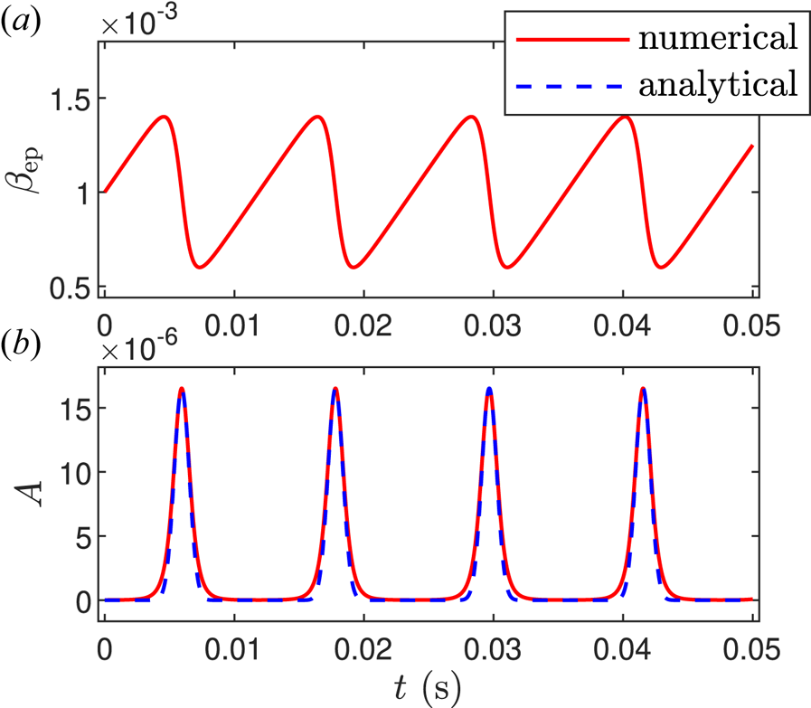
This analytical solution has been verified numerically as shown in figure 1, where the red line is the numerical solution of (2.1) and (2.2) and the blue dashed line is the analytical solution of (2.8). The five free parameters are selected as $\beta _{\rm {crit}}=0.001$, $\beta _{\rm {max}}=0.0014$, $\varGamma =5.0\times 10^6\,\mathrm {s}^{-1}$, $D=0.1\,\mathrm {s}^{-1}$ and $Z=3.0\times 10^7\,\mathrm {s}^{-1}$, which come from the fitting of EAST experimental data (Xu et al. Reference Xu, Zhang, Chen, Hu, Li, Lin, Shi, Duan and Zhu2015; Zhu et al. Reference Zhu, Zeng, Qiu, Hao, Shen, Gu, Wu, Tang, Qian and Liu2020). The initial conditions are $\beta _{\rm {ep}}=\beta _{\rm {crit}}$ and $A=A_{\rm {min}}$. The maximum $A_{\rm {max}}$ in the numerical solution is exactly the same as the value calculated from (2.4) and (2.5). Meanwhile, the burst period $t_p$ and the burst width $\Delta t$ both coincide with the numerical solution.

Figure 1.

Numerical solution (red line) of (2.1) and (2.2), analytical solution (blue dashed line) of (2.8), where the burst period $t_p$ and width $\Delta t$ are defined in (2.6) and (2.7b), respectively.

2.2. Poloidal rotation driven by EP radial current

It can be shown that (2.1) is essentially the EP transport equation. The flux surface averaged EP charge conservation law is

(2.9)\begin{equation} \frac{\partial \rho_{\rm{ep}}}{\partial t}+\frac{1}{r}\frac{\partial}{\partial r}(rJ_r)=S_{\rm{ep}}, \end{equation}

where $\rho _{\rm {ep}}\equiv q_{\rm {ep}}n_{\rm {ep}}$, $q_{\rm {ep}}$ and $n_{\rm {ep}}$ are the EP charge and density, respectively, $J_r$ is the radial current, $r$ is radial coordinate (the simple toroidal coordinate system is adopted and $r$ represents the flux surface) and $S_{\rm {ep}}$ is the source of EPs. Assuming the radial current comes from interaction of EPs and fishbone, its radial structure can be represented by a Gaussian shape as computed by HAGIS simulations (Pinches et al. Reference Pinches, Günter and Peeters2001),

(2.10)\begin{equation} J_r(r,t)\approx J(t)\frac{r}{r_0}\exp\left[-\left(\frac{r-r_0}{\Delta r}\right)^2\right], \end{equation}

where $r_0$ is the position of the Gaussian peak which mostly depends on the location in phase space of the dominant precessional resonant response (Fu et al. Reference Fu, Park, Strauss, Breslau, Chen, Jardin and Sugiyama2006). In practice, $r_0\sim r_s$ is the position of $q=1$ surface and $\Delta r\sim r_s$ is the radial width of fishbone. The Gaussian shape used here is just to simplify the model calculation: one can substitute a realistic profile of $J_r$ into simulations or experiments to obtain more precise results. Multiplying by $4\mu _0T_{\rm {ep}}r/B^2_0q_{\rm {ep}}r^2_s$ and integrating from $0$ to $r_s$ in (2.9), we get

(2.11)\begin{equation} \frac{{\rm d}\beta_{\rm{ep}}}{{\rm d}t}=D-\frac{4\mu_0T_{\rm{ep}}}{B^2_0q_{\rm{ep}}r_s}J(t), \end{equation}

where $\beta _{\rm {ep}}\equiv 2\mu _0\bar {n}_{\rm {ep}}T_{\rm {ep}}/B^2_0$ is the averaged EP beta, $\bar {n}_{\rm {ep}}\equiv \int _0^{r_s}2rn_{\rm {ep}}\,{\rm d}r/r^2_s$ is the averaged EP density, $T_{\rm {ep}}$ is the EP temperature and is assumed to be a constant, $\mu _0$ is the permeability of vacuum and $D\equiv (4\mu _0T_{\rm {ep}}/B^2_0 q_{\rm {ep}}r^2_s)\int _0^{r_s}S_{\rm {ep}}r\,{\rm d}r$. Comparing with (2.1), one can identify that the radial current is proportional to the fishbone amplitude,

(2.12)\begin{equation} J(t)=J_fA(t), J_f\equiv \frac{B^2_0 q_{\rm{ep}}r_s}{4\mu_0T_{\rm{ep}}}Z\beta_{\rm{max}}. \end{equation}

There is also a theoretical derivation from the nonlinear gyrokinetic equation (Zonca et al. Reference Zonca, Buratti, Cardinali, Chen, Dong, Long, Milovanov, Romanelli, Smeulders and Wang2007), confirming the linear relation between fishbone amplitude and EP transport flux.

The equation for poloidal rotation driven by radial current (Peeters Reference Peeters1998) is derived in Appendix A as

(2.13)\begin{equation} a\frac{\partial V_{\theta}}{\partial t}={-}\nu V_{\theta}-fJ_r, \end{equation}

where $a=(\epsilon ^2/q^2)(1+2q^2+1.63q^2/\sqrt {\epsilon })$, $1.63q^2/\sqrt {\epsilon }$ comes from the neoclassical effect (Shaing, Ida & Sabbagh Reference Shaing, Ida and Sabbagh2015), the poloidal flow damping rate $\nu =1.1\nu _{ii}\sqrt {\epsilon }$ is proportional to the ion–ion collisional frequency $\nu _{ii}$, $f=(\epsilon ^2/q^2)(B_0/n_im_i)$, $n_i$ and $m_i$ are the ion density and mass, respectively, $\epsilon \equiv r/R_0$ and $R_0$ is major radius of the tokamak. As the radial current $J(t)\propto A(t)$, which is composed of successive bursts, a steady poloidal flow can be built up on condition that the burst frequency is greater than the poloidal flow damping rate. The steady flow for a given radial position can be estimated as follows: here we choose the position of $r=r_s$ for illustration, for other positions near $r=r_s$, the conclusion is qualitatively the same. For $r=r_s$, vanishing of the left-hand side of (2.13) gives the steady solution

(2.14)\begin{equation} \left\langle V_{\theta}\right\rangle_t={-}\frac{f}{\nu}\left\langle J_r\right\rangle_t={-}\frac{f}{\nu}J_f\left\langle A(t)\right\rangle_t, \end{equation}

where $\left \langle \cdots \right \rangle _t$ denotes the long-time average, and is equivalent to the time average over one period, $\left \langle A(t)\right \rangle _t=\int _0^{t_p}\,{\rm d}tA_s(t)/t_p$. For $\Delta t\leq t_p$, the integral $\int _0^{t_p}\,{\rm d}tA_s(t)$ is close to Gaussian integral and $\approx \sqrt {{\rm \pi} }\Delta t A_{\rm {max}}$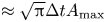. As a result, the steady flow can be approximated as

(2.15)\begin{equation} \left\langle V_{\theta}\right\rangle_t\approx{-}\sqrt{\rm \pi}\frac{\Delta t}{t_p}\frac{f}{\nu}J_fA_{\rm{max}}. \end{equation}

It can be shown that the steady flow is proportional to $\Delta t/t_p$, which means the larger burst frequency or the longer burst duration would lead to larger steady flow shear and assist in the building of ITB. In order to calculate the radial shear of the poloidal rotation, (2.13) and its radial derivative are written respectively as

(2.16)\begin{gather} \frac{\partial V_{\theta}}{\partial t}={-}\frac{\nu}{a}V_{\theta}-\frac{f}{a}J_r, \end{gather}

(2.17)\begin{gather} \frac{\partial V^{\prime}_{\theta}}{\partial t}={-}\frac{\nu}{a}V^{\prime}_{\theta}-\left(\frac{\nu}{a}\right)^{\prime}V_{\theta}-\frac{f}{a}J^{\prime}_r-\left(\frac{f}{a}\right)^{\prime}J_r, \end{gather}

where the prime represents derivative in the radial direction. The flow shear $V^{\prime }_{\theta }$ can be obtained by solving (2.16) and (2.17) simultaneously. Here we only consider the radial variation of $\epsilon$ in the coefficients $a$, $\nu$ and $f$; the equilibrium related parameters such as $q$, $\nu _{ii}$ and $n_i$ are assumed to be constant. Since the leading-order term for $\epsilon \ll 1$ in $a$ is $1.63q^2/\sqrt {\epsilon }$, we have $a^{\prime }/a \approx 3/2r$, $\nu ^{\prime }/\nu =1/2r$ and $f^{\prime }/f=2/r$. The steady flow shear can be estimated by the same method given previously, for $r=r_s$, vanishing of the left-hand side of (2.17) gives

(2.18)\begin{equation} \left\langle V^{\prime}_{\theta}\right\rangle_t\approx{-}\frac{5\sqrt{\rm \pi}}{2r_s}\frac{\Delta t}{t_p}\frac{f}{\nu}J_fA_{\rm{max}}. \end{equation}

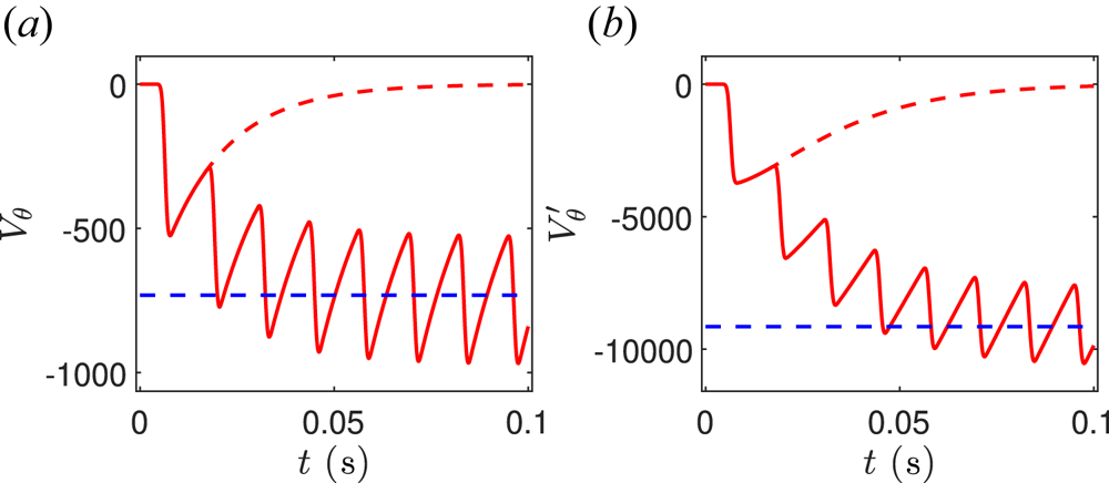
Selecting a set of typical tokamak parameters such as $R_0=2\,{\rm m}$, $r_s/R_0=0.1$, $\nu =5\,{\rm s}^{-1}$ and $fJ_f=2.0\times 10^9\,{\rm m}\,{\rm s}^{-2}$, the numerical solution of (2.16) and (2.17) is displayed in the red line in figure 2(a,b) and the dashed blue line is the analytical steady solution of (2.15) and (2.18), respectively. The poloidal rotation driven by a single burst of (2.7a) is also displayed as a dashed red line, and is eventually damped without a steady flow. Note that similar results have been obtained in figure 4 of Pinches et al. (Reference Pinches, Günter and Peeters2001).

Figure 2.

(a) Numerical solution (solid red line) of (2.16), where the dashed blue line is the analytical solution of (2.15). (b) Numerical solution (solid red line) of (2.17), where the dashed blue line is the analytical solution of (2.18) and the dashed red line is the poloidal rotation driven by a single burst of (2.7a).

Substituting (2.12) into (2.18) gives an analytical expression to estimate the absolute value of the steady flow shear induced by fishbone bursts,

(2.19)\begin{equation} \left\langle \left|V^{\prime}_{\theta}\right| \right\rangle_t\approx\frac{5\sqrt{\rm \pi}}{8.8}\frac{\epsilon^{3/2}}{q^2}\frac{\varOmega_{\rm{ep}}}{\nu_{ii}}\frac{v^2_A}{v^2_{\rm{ep}}}\frac{\Delta t}{t_p}Z\beta_{\rm{max}}A_{\rm{max}}, \end{equation}

where $v_A\equiv B_0/\sqrt {\mu _0n_im_i}$ is the Alfvén velocity, $v_{\rm {ep}}\equiv \sqrt {T_{\rm {ep}}/m_{\rm {ep}}}$ is the EP thermal velocity, $\varOmega _{\rm {ep}}\equiv q_{\rm {ep}}B_0/m_{\rm {ep}}$ is the EP gyrofrequency. This quantitative formula can be further simplified when $D$ is small enough, $D\ll A_{\rm {max}}Z\beta _{\rm {max}}$. By using the relations given by (2.5)–(2.7a,b), the burst width can be approximated as $\Delta t\approx \sqrt {2/(\varGamma A_{\rm {max}}Z\beta _{\rm {max}})}$, because most of the time $A\ll A_{\rm {max}}$, the $AZ\beta _{\rm {max}}$ term in the integrand of (2.6) can be neglected; hence, the integral is solved analytically, $t_p\approx 2\sqrt {2A_{\rm {max}}Z\beta _{\rm {max}}/\varGamma }/D$. As a result, we obtain $\Delta t/t_p\approx D/(2A_{\rm {max}}Z\beta _{\rm {max}})$ and

(2.20)\begin{equation} \left\langle \left|V^{\prime}_{\theta}\right| \right\rangle_t\approx\frac{5\sqrt{\rm \pi}}{17.6}\frac{\epsilon^{3/2}}{q^2}\frac{\varOmega_{\rm{ep}}}{\nu_{ii}}\frac{v^2_A}{v^2_{\rm{ep}}}D, \end{equation}

which means that the steady flow shear grows linearly with $D$ increasing, and it is independent of other parameters of $Z,\beta _{\rm {crit}},\beta _{\rm {max}},\varGamma$. This analytical expression is broken as $D\rightarrow A_{\rm {max}}Z\beta _{\rm {max}}$, since $\Delta t\rightarrow \infty$ as shown in (2.7b). In fact, when $\Delta t>t_p$, the solution of $A$ behaves like oscillation rather than burst; thus, the form of exponential in (2.7a) is incorrect. However, the numerical solution in § 3 still shows the same trend that the steady flow shear only depends on $D$ linearly.

2.3. Ion transport model

The temporal evolution of ion temperature gradient mode (ITG) fluctuation level and ion pressure gradient can be described by a simple zero-dimensional model (Diamond et al. Reference Diamond, Lebedev, Newman, Carreras, Hahm, Tang, Rewoldt and Avinash1997; Newman et al. Reference Newman, Carreras, Lopez-Bruna, Diamond and Lebedev1998),

(2.21)\begin{gather} \frac{\partial E}{\partial t}=\left(\gamma_0N-\alpha_1E-\alpha_2V^{\prime2}_E\right)E, \end{gather}

(2.22)\begin{gather} \frac{\partial N}{\partial t}=S-(D_n+D_aE)N, \end{gather}

where $E\equiv \left \langle (\tilde {n}/n)^2 \right \rangle ^{1/2}$ is the normalised turbulent fluctuation level and $N\equiv (a_0/P_i)(-{\rm d}P_i/{\rm d}r)$ is the ion pressure gradient normalised with the minor radius $a_0$. The parameter $\alpha _1$ is determined by the saturation level of the instability in the low-confinement regime and can be estimated by the empirical mix-length model (Diamond et al. Reference Diamond, Lebedev, Newman and Carreras1995), $\gamma _0/\alpha _1\sim \Delta _r/a_0$. The other parameter $\alpha _2$ is determined from the $E\times B$ shear flow suppression criterion (Biglari, Diamond & Terry Reference Biglari, Diamond and Terry1990; Zhang & Mahajan Reference Zhang and Mahajan1992), $\alpha _2=(\Delta _r/\Delta _{\theta })^2/\gamma _0$. Here, $\Delta _r$ and $\Delta _{\theta }$ are the turbulent radial and poloidal correlation length, respectively, and assumed to be the same order, $\Delta _r\approx \Delta _{\theta }$. Here $S$ is the source of thermal ions, and $D_n$ and $D_a$ are the neoclassical and turbulent transport coefficients, respectively. The $E \times B$ flow $V_E$ is determined by the radial ion force balance equation,

(2.23)\begin{equation} V_E=V_{\theta}-\frac{B_{\theta}}{B}V_{\varphi}-\frac{1}{eBn_i}\frac{{\rm d}P_i}{{\rm d}r}. \end{equation}

In this paper, we focus on the poloidal rotation induced by fishbone. Neglecting the toroidal rotation $V_{\varphi }$ and ion pressure gradient term in (2.23) leads to $V^{\prime }_E\approx V^{\prime }_{\theta }$. As a result, the predator–prey model and the ion transport model are coupled through the sheared poloidal flow term in (2.21).

There are two steady solutions for (2.21) and (2.22): (a) low-confinement solution $(E,N)=(E_L,N_L)$, when the flow shear $V^{\prime }_{\theta }\approx 0$, the saturation level of the turbulent fluctuation is $E_L=\gamma _0 N_L/\alpha _1$, and the steady transport satisfies $S=(D_n+D_aE_L)N_L$; and (b) high-confinement solution $(E,N)=(E_H,N_H)$, when the flow shear is larger than a critical value, the turbulent fluctuation is suppressed, $E_H\approx 0$, the transport is neoclassical, $N_H=S/D_n$. The critical value of flow shear is

(2.24)\begin{equation} \left|V^{\prime}_{\theta}\right|\geq V^{\prime}_{\theta,c}\equiv \gamma_0\sqrt{S/D_n}. \end{equation}