1. Introduction

The collection and compilation of an increasing number of field measurements in Antarctica is leading to a depiction of the spatial distribution of the long-term mean surface mass balance (Reference Vaughan, Bamber, Giovinetto, Russell and RVaughan and others, 1999; Reference Giovinetto and ZwallyGiovinetto and Zwally, 2000) which, although still questionable in various regions and respects (Reference Genthon and KrinnerGenthon and Krinner, 2001), is now probably largely realistic. The intra-annual variability, and in particular the seasonal cycle, of the Antarctic precipitation or surface accumulation (the latter equivalent to surface mass balance here) has been addressed in various ways (e.g. Reference BromwichBromwich, 1988) and more recently by meteorological and climate models (e.g. Reference Cullather, Bromwich and Van WoertCullather and others, 1998; Reference Genthon, Krinner and DéquéGenthon and others, 1998; Reference Genthon and KrinnerGenthon and Krinner, 1998) because direct observations on the field are both too sparse and generally insufficiently reliable for this purpose. For the evaluation of interannual variability, field records of precipitation as well as glaciological measurements such as snow pits, ice cores and stake networks may provide valuable data (e.g., as reported in Reference Rémy, Testut and LegrésyRémy and others, 2002). However, these are local evaluations, the spatial significance of which may be obscured by small-scale spatial variability and has not been comprehensively evaluated. Meteorological and climate models ignore subgrid spatial variability and provide estimates at the gridscale and more, that is, a few tens of km to a few hundred km for Antarctica at this time. A study of the modes of interannual variability of precipitation in the Antarctic region has recently been carried out on the basis of meteorological analyses and climate model results (Reference Genthon, Krinner and SacchettiniGenthon and others, 2003). Here, model results are further used to evaluate the space–time structure of this interannual variability.

Large-scale space–time statistics of precipitation are expected to contribute to assessing the spatial significance of, and extrapolating, local and regional measurements in the field. The space–time structure of accumulation is also needed to determine how exploitable satellite altimetry is for volumetric monitoring of the ice sheet (e.g. in relation to climate change). Reference Rémy, Testut and LegrésyRémy and others (2002) show that the large time-scale of relaxation of an ice sheet induces low-frequency responses to random fluctuations of snow accumulation. From broad estimates of the variability of accumulation, they report that the amplitude of the induced variance of ice elevation may be as high as 10 m on 30 year time-scales. The perturbation affects more particularly the coastal regions. Since air temperatures are higher and accumulation rates are substantially greater than in the interior, climate change has the potential to alter mass balance in the coastal areas more rapidly than inland (ISMASS Committee, 2004). The areas of strongest volumetric response to climate change are thus also those most exposed to noise induced by accumulation variability. It is essential that the characteristics of this noise be determined, and this requires large-scale information on precipitation/accumulation variability on interannual, decadal and longer time-scales. This requirement includes information on spatial covariability, which affects the dynamic response of the ice as well as the determination of the current mass balance of the ice sheet (Reference WinghamWingham, 2000).

Recent meteorological and climate models, although still prone to many kinds of defects and shortcomings, have been shown to reproduce the mean accumulation of Antarctica relatively well (Reference Genthon and KrinnerGenthon and Krinner, 2001). Meteorological analyses and the results from high-resolution atmospheric general circulation models are the a priori preferred model data for an analysis of variability, but the available series cover a few decades at best. This is too short a period to adequately sample variability beyond the interannual time-scale. Thus, here, results from coarser coupled ocean– atmosphere climate models are also used to evaluate the amplitude of interannual variability and tentatively relate it to the interdecadal time-scales. This is done in section 2. In section 3, the space–time structure of precipitation/accumulation from meteorological analyses and climate models over Antarctica is presented and discussed. In section 4, a coarse evaluation of the potential of mechanical post-depositional processes (wind erosion and blowing snow) to affect surface mass-balance statistics is made. A summary and conclusion is provided in section 5.

2. Interannual to Interdecadal Variability

Because they are constrained by observations in the atmosphere and/or at the sea-surface boundary conditions, meteorological analyses (or, in the case of precipitation or accumulation, short-term forecasts from meteorological analyses) and atmospheric general circulation models (AGCMs) may be expected to yield the most realistic information on variability. Coupled atmosphere–ocean general circulation models (AOGCMs) may be more biased since they have more degrees of freedom, but they can be run over long periods of time and thus provide samples for evaluation of variability at interdecadal and longer time-scales. Here, we use 240 year simulations by two AOGCMs, the HADCM3 model from the Hadley Center for Climate Prediction and Research, UK, and the ECHAM4/OPYC3 model from the Deutsches Klimarechenzentrum DKRZ, Germany, both at ∼300km horizontal resolution. These simulations are reference current climate runs with constant CO₂ and other atmospheric forcing. The data are described by, and available from, the Intergovernmental Panel on Climate Change (IPCC) Data Distribution Center (http://ipcc-ddc.cru.uea.ac.uk/).

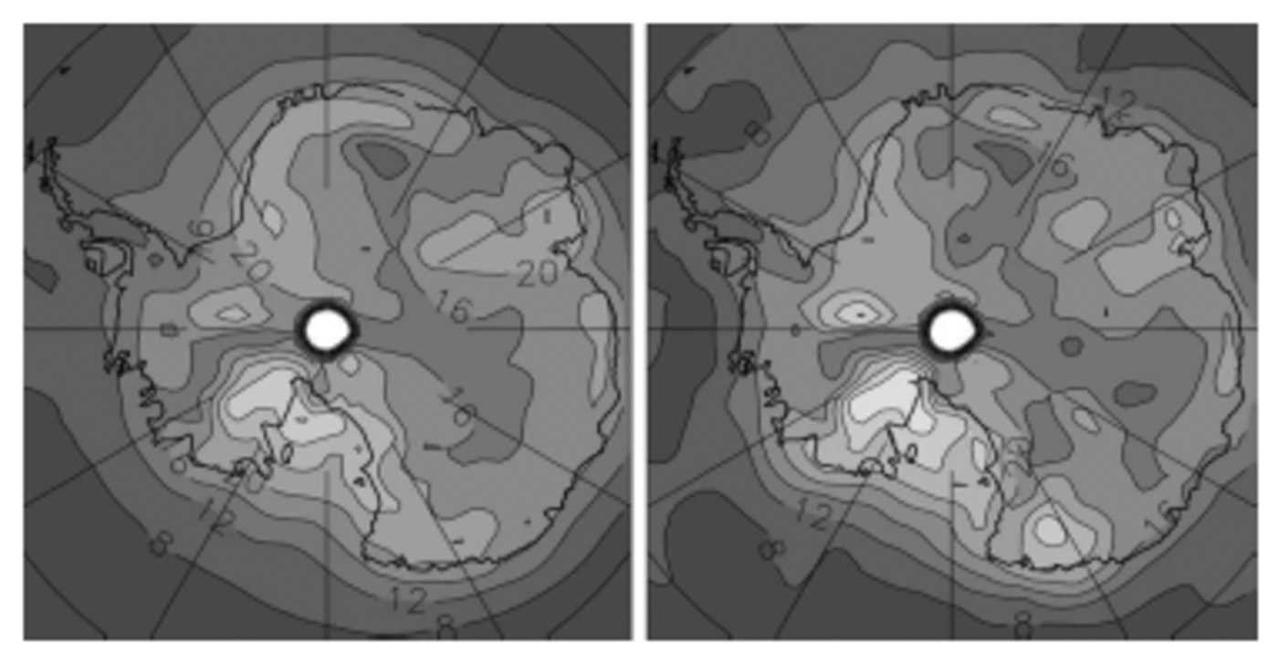
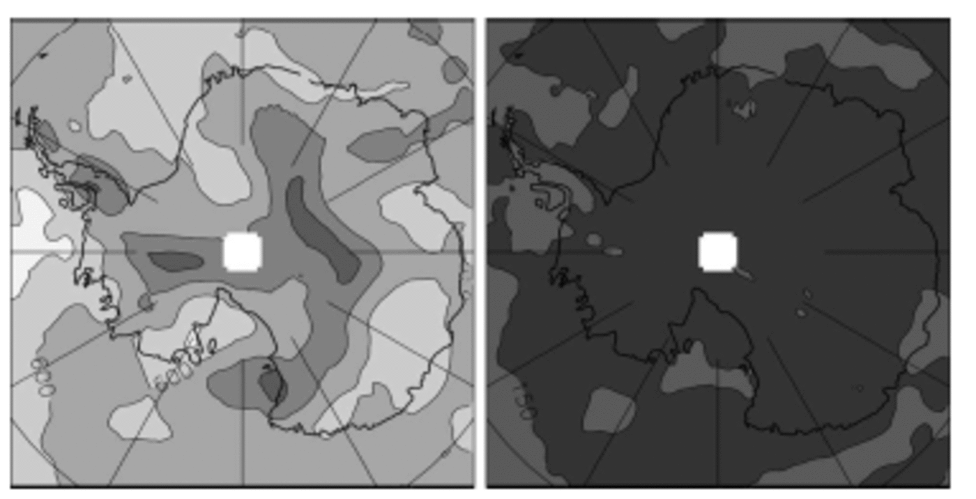
Figure 1 shows the relative standard deviation (SD) of precipitation from HADCM3 after the monthly time series of precipitation for each model gridbox have been averaged over consecutive intervals of 1 (interannual) and 10 (interdecadal) years. As expected, the amplitude of variability decreases as the time sampling/averaging increases, here in a way which is largely consistent with a ‘white’ random noise. This is demonstrated in Figure 1 by the fact that the maps of interannual and interdecadal relative SD are very similar if the latter is multiplied by 10^1/2.

Fig. 1.

Interannual (left) and interdecadal (right, multiplied by 10^1/2 = 3.16) relative standard deviation of precipitation, in %, for the 240 year HADCM3 AOGCM simulation. Contour interval: 4%. Lighter grey = larger values. Colour version available at http://lgge.obs.ujf-grenoble.fr/ ~christo/antvar/index.htm.

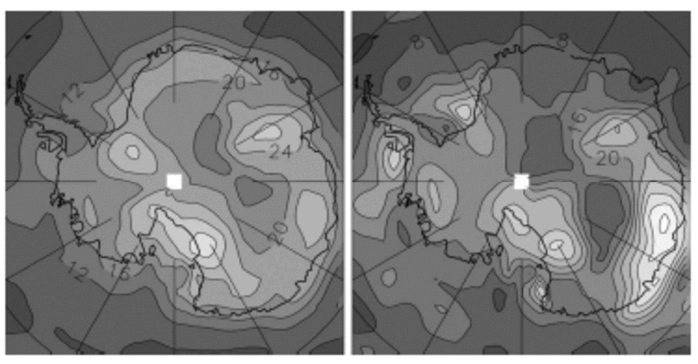
However, the variability of precipitation in the ECHAM4/OPYC3 AOGCM decreases less rapidly with time sampling/averaging than a white random noise would (Fig. 2; note that the interdecadal relative SD is multiplied by only 2, that is, <10^1/2), and is thus significantly ‘red’. The spatial distribution of the relative SD is also somewhat more sensitive to time-scale, i.e. a lesser decrease with time sampling in Wilkes Land than elsewhere, yet it remains broadly conserved over much of the ice sheet. Although an evaluation of the variability of precipitation at interannual time-scales may lead to a significant underestimation of the variability at longer time-scales, if white randomness is assumed, it is nonetheless likely to provide fairly reasonable evaluations of the space–time structure of this variability, even at long time-scales.

Fig. 2.

Interannual (left) and interdecadal (right, multiplied by 2) relative standard deviation of precipitation, in %, for the 240 year ECHAM4/OPYC3 AOGCM simulation. Contour interval: 4%. Lighter grey = larger values (colour version: see Fig. 1 caption).

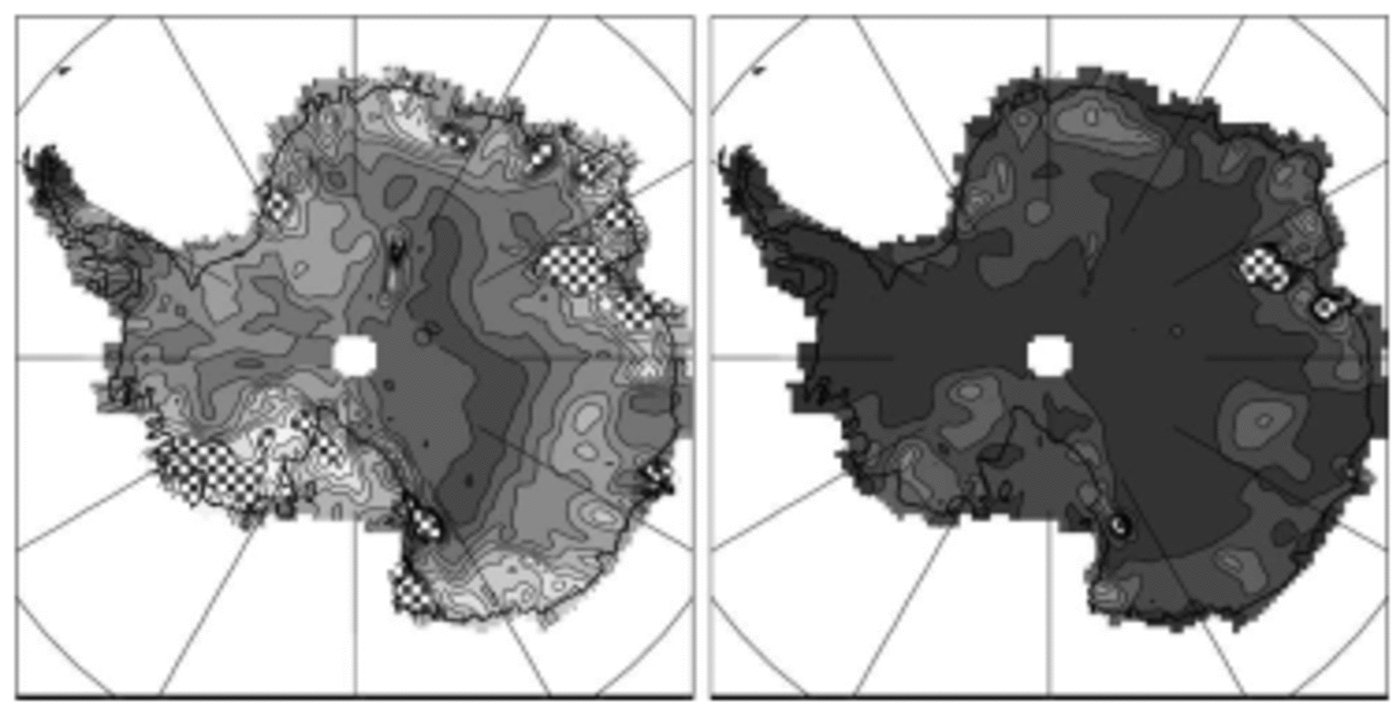
Evaporation from the two AOGCMs is not available, so we now turn to a 21 year simulation by the LMDZ high Antarctic resolution (∼100 km) AGCM (Reference Genthon, Krinner and CosmeGenthon and others, 2002) in order to evaluate the contribution of sublimation to surface mass-balance variability. Concerning sublimation, models significantly disagree with each other (Reference Genthon and KrinnerGenthon and Krinner, 2001), and the LMDZ model is not necessarily more reliable than others in this respect. We thus use this model here to illustrate, rather than quantify, that the contribution of sublimation to the variability of accumulation is probably limited. Figure 3 shows the interannual relative SD of precipitation from the LMDZ model, which largely agrees with the other models (Fig. 1 and 2). Figure 3 also shows the relative contribution of sublimation to the variability of the surface mass balance. This is quite low, mostly <5% on the ice sheet. Much of the absolute variability of accumulation originates from the variability of precipitation, with negligible contribution from sublimation. However, sublimation may enhance the relative variability of surface mass balance without significantly affecting the absolute variability, where it reduces accumulation to very low values, that is where much of the deposited precipitation sublimates. Again, models do not generally agree well with each other, and with observation-based estimates, to determine regions of high sublimation over precipitation ratio.

Fig. 3.

Interannual relative SD of precipitation (left), and relative contribution of evaporation to the surface mass-balance variability (right), in %, for the LMDZ AGCM. Contour interval: 4%. Lighter grey = larger values (colour version: see Fig. 1 caption).

Thus, to minimize uncertainties specific to a single model: (i) we average the absolute interannual SD of precipitation from four datasets, the two AOGCMs, the LMDZ AGCM and also the 15 year European Centre for Medium-RangeWeather Forecasts (ECMWF) ERA15 re-analysis-based precipitation (∼100km resolution; Reference Gibson, Kållberg, Uppala, Hernandez, Nomura and SerranoGibson and others, 1997; Reference Genthon and KrinnerGenthon and Krinner, 1998); (ii) we assume that the contribution of sublimation to the variability of the surface mass balance is weak and can be ignored; and (iii) we normalize by the Reference Vaughan, Bamber, Giovinetto, Russell and RVaughan and others (1999) observation-based estimate of surface mass balance, to obtain the mean relative SD. The result is shown in Figure 4, along with the inter-model SD as a measure of the degree of agreement between the four datasets used. The spots of high relative SD (stippled) are areas of low accumulation in the Reference Vaughan, Bamber, Giovinetto, Russell and RVaughan and others (1999) map and are not associated with particularly high variability of precipitation (see Fig. 1–3). These are typically areas of largest systematic disagreement with climate models (Reference Genthon and KrinnerGenthon and Krinner, 2001), possibly reflecting systematic deficiencies of the models (e.g. related to blowing snow (section 4)), or revealing shortcomings in the Reference Vaughan, Bamber, Giovinetto, Russell and RVaughan and others (1999) compilation and extrapolation of observations. While the possibility that some of these high values of relative variability are realistic should be kept in mind, in many respects they are of relatively limited consequence since they are geographically localized (but not so in Marie Byrd Land), and they are associated with low surface mass balance according to Reference Vaughan, Bamber, Giovinetto, Russell and RVaughan and others (1999).

Fig. 4.

Interannual relative SD of precipitation as averaged from ECHAM4/OPYC3, HADCM3, LMDZ and ERA15 precipitation and normalized to Reference Vaughan, Bamber, Giovinetto, Russell and RVaughan and others (1999) accumulation (left), and corresponding inter-model SD (right), in %. Contour interval: 4%. Lighter grey = larger values. Regions with values in excess of 40% are stippled (colour version: see Fig. 1 caption).

On average over the ice sheet, the mean relative variability is ∼20% if stippled spots in Figure 4 (left) are ignored (∼30% if they are taken into account). Compiling various sources of observation, Reference Rémy, Testut and LegrésyRémy and others (2002) report interannual variability of accumulation ranging from 15% to 45%, slightly above the model results reported here. However, to evaluate the impact of this variability on the significance of surface altimetry measurements, Reference Rémy, Testut and LegrésyRémy and others (2002) elect to use 10–15% of variability when averaged over 30 years. Thus, they assume that the variability has a red rather than white spectrum, possibly an overestimation on the basis of the HADAM3 AOGCM results, but not on the basis of those from the ECHAM4/OPYC3 model. Observations at various sites (Reference GoodwinGoodwin, 1991; Reference Mosley-Thompson, Paskievitch, Gow and ThompsonMosley-Thompson and others, 1999) confirm that 10–15% of relative SD on decadal and longer time-scales is not unreasonable. However, it should be kept in mind that field observations provide local measurements of accumulation. Estimates of time variability from such measurements mix the contribution of all spatial scales, including scales which models cannot account for since they are subgrid (i.e. less than ∼100 km for the finest models here). Thus, it is not unexpected that models provide somewhat smaller estimates of variability than observations. Actually, for various applications including the impact of short-term accumulation variability on long-term surface elevation changes, the scales resolved by models may be more appropriate than those over which local observations are relevant.

3. Spatial Radius of Decorrelation (RD)

The space–time structure of variability is evaluated through the radius of decorrelation (RD). RD is the horizontal distance across which two time series of precipitation may be expected to contain ‘significantly’ common variability, as indicated by their linear correlation. Here, this distance is assumed to be isotropic and is thus evaluated as the radius of a circle. This is not necessarily true everywhere as, for instance, correlations may be larger along main pathways of advection by the atmosphere, or lower across topographic ridges. Thus, the results and maps shown here may need refinement for specifically detailed applications. However, an isotropic measure provides a synthetic picture at the full scale of Antarctica. A linear correlation of 0.7 indicates that two series share about 50% of common variability. Thus, RD is calculated here as the radius of the circle within which the correlation between all available (depending on the model grid) time series is on average 0.7. This is admittedly somewhat arbitrary. Yet, the global-mean interannual RD from the various models used here ranges from ∼400 to ∼600 km, on average ∼500 km, and this agrees with other approaches to evaluating the spatial significance of observed precipitation time series at interannual time-scales (Reference RubelRubel, 1996).

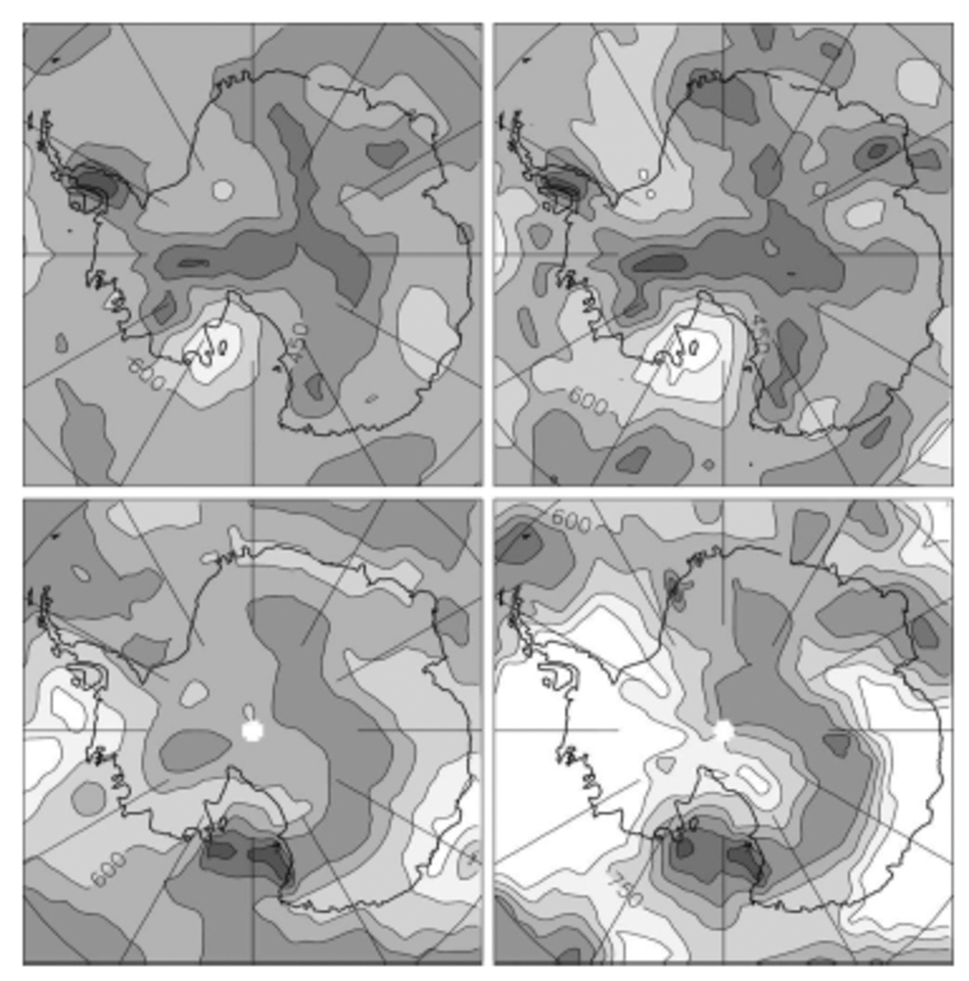
Figure 5 shows the distribution of RD over Antarctica for the HadCM3 and ECHAM4/OPYC3 AOGCMs, with the available monthly time series averaged over 1 year (interannual RD) or 10 year (interdecadal RD) intervals (any value of RD below mean model resolution, i.e. ∼300km here, should be considered of limited or no significance). As expected from results in section 2, the maps of RD are largely independent of time-scale for the first model, less so for the second one. Thus the interannual RD may be expected to reflect, or to somewhat underestimate, RD at the longer time-scales, the spatial patterns being largely conserved. Figure 6 shows the inter-model mean RD, as averaged from the individual interannual precipitation RD of ECHAM4/OPYC3, HADCM3, LMDZ and ERA15. The model-average values range spatially from <300km (close to the coarser-models resolution) to >700 km, with a mean radius of ∼500km and a mean correlation circle surface of ∼850 000km² on the ice sheet. Because the surface of the grounded ice sheet is ∼12 400 000km², this result indicates that there are at least ∼15 independent precipitation basins in Antarctica.

Fig. 5.

Radius of decorrelation (in km) of precipitation for the HADCM3 (upper plots) and ECHAM4/OPYC3 AOGCMs (lower plots), on interannual (left plots) and interdecadal (right plots) time-scales. Contour interval: 150 km. Lighter grey = larger values (colour version: see Fig. 1 caption).

Fig. 6.

Inter-model mean (left) and standard deviation (right) of the RD of precipitation from ECHAM4/OPYC3, HADCM3, LMDZ and ERA15, in km. Contour interval: 150 km. Lighter grey = larger values (colour version: see Fig. 1 caption).

The inter-model SD of RD is mostly <150km (Fig. 6). Thus, the model and analysis data agree relatively well with each other, in terms both of spatial pattern and of mean values. Interestingly, lower values appear to parallel the main ridges of the ice sheet although they do not exactly coincide with the ridges. Thus, although quite smooth, the interior topography may significantly affect the space–time structure of the precipitation. RDs are generally larger at or near the coasts than inland, probably reflecting the relatively large-scale influence of coastal and offshore frontal systems.

The results reported above are marginally affected when evaporation is taken into account to estimate the RD of accumulation. We are not aware of observations that allow even partial verification of these results. Correlating observed series of accumulation at interannual to interdecadal time-scales over distances of several hundred km implies that the contribution of the small (i.e. cm to hundreds of km) and larger scales to temporal variability can be sorted out. This is not generally the case, and in fact our results are meant to help in this respect. The ITASE (International Trans-Antarctic Scientific Expedition, http://www.ume.maine.edu/itase/toc.html) programme, a major international initiative to provide complete and high-resolution exploration of the surface of the ice sheet, could deliver essential data if not only the mean accumulation, but also its recent variability at time-scales down to interannual, is systematically evaluated along the traverses.

4. Wind Effects

The contribution of blowing/drifting snow to the surface mass balance of the Antarctic ice sheet (Reference BintanjaBintanja, 1998; Reference GalléeGallée, 1998), through both exporting and enhancing sublimation of airborne ice particles (here together summarized as wind effects), is still poorly known. It is currently not simulated by climate models. Therefore, data to properly estimate the interannual variability and space–time structure of accumulation including wind effects are (to our knowledge) not available. Because the processes associated with blowing snow are complex and highly non-linear, only a very coarse evaluation, based on surface winds, is given here. Figure 7 shows the interannual relative SD and the RD of the surface wind intensity from the LMDZ model. The interannual variability is low, mostly <5% except at the coasts and along the topographic ridges on the high plateau. This is probably because the surface wind is largely conditioned by slopes and gravity (katabatic winds) and, thus, has relatively high interannual constancy, except where it is also affected by synoptic disturbances (coasts) or where the slopes are minimal (ridges, domes). On the other hand, wind variability is relatively decorrelated in space: RD = ∼350km on average over the Antarctic ice sheet, suggesting >30 separate wind basins. Otherwise, the general spatial structure of the wind RD is rather similar to that of precipitation (Fig. 6), except for very low values of the former right at the coasts. Thus, if the space–time statistics of wind effects are reflected by surface wind, they may somewhat amplify those of precipitation alone but not modify the general spatial pattern, except in narrow coastal bands.

Fig. 7.

Interannual relative SD (left) and RD (right) of surface wind intensity in the LMDZ model. Contour interval: 4% (left) or 150 km (right). Lighter grey = larger values (colour version: see Fig. 1 caption).

Although there is no simple linear relation between surface wind intensity and snow erosion, transport and sublimation, the extra accumulation variability induced by wind effects is unlikely to be much larger than the mean wind effects themselves. Estimates from offline models (Bintanja, 1998) and from short-term regional climate model simulations (Reference GalléeGallée, 1998) suggest that, except very locally, wind effects do not erode >25% of the deposited snow. Thus, estimates of the space–time statistics of the surface mass balance from precipitation alone (Fig. 4 and 6) are possibly somewhat, but unlikely strongly, underestimated.

5. Discussion and Conclusion

We have provided estimates of the interannual to interdecadal variability and spatial correlations of the surface mass balance of Antarctica. In particular, we show maps of the relative standard deviation of precipitation which, on interannual time-scales, ranges from ∼5% in the remotest interior to ∼40% and possibly more closer to the coasts. We also find that this variability is spatially coherent at distances of ∼500km on average, less in the interior, and in excess of 700 km in various regions. We find that interannual statistics can be extrapolated to interdecadal time-scales as far as the spatial distribution is concerned, but that the amplitude of variability and spatial coherence may then be somewhat underestimated. These results are obtained from meteorological analyses and from climate models, at this time the only source of data with sufficient spatial and temporal coverage for such purpose. Our estimates should provide useful hints as to where field measurements are most critical and needed to build an exhaustive observation-based understanding of the surface mass balance of Antarctica (e.g. as part of the ongoing ITASE programme). Also, as new instruments will soon be or have been recently launched for an accurate monitoring of the ice-sheet surface elevation from space (e.g. ISMASS Committee, 2004), these estimations are essential for an appropriate interpretation of such altimetric measurements (Reference WinghamWingham, 2000; Reference Rémy, Testut and LegrésyRémy and others, 2002).

Conversely, real data are needed to verify and improve the model-based analysis presented here. While models physically account for the main process of accumulation, that is precipitation, they may not do so with unquestionable realism. Antarctic precipitation is the result of a mixture of processes. Some are common in other regions (e.g. frontal precipitation, at the coasts of the ice sheet), benefit from global model verification and adjustments, but are prone to deficiencies similar (and rather common) to those in other regions. Others, like clear-sky condensation, in association with subsidence of relatively moist air into the cold boundary layer, are more specific to the Antarctic Plateau and may not be well evaluated. Although evaporation/sublimation is also physically treated in the climate models, it is clear, by simply comparing the models with each other, that it is not consistently well reproduced. Other processes that contribute to the surface mass balance (e.g. blowing snow) are simply ignored. We have attempted to evaluate the uncertainties associated with inaccurately treated or missing processes in models, but they remain a substantial source of uncertainties. These may be reduced in the future through improvements to the models, but such improvements can be validated only if relevant real data are available. While an increasing number of field data are available to characterize the mean surface mass balance of Antarctica, it is essential that the variability is also addressed, in a much more extensive way than done so far.

It is very unlikely that field data will soon become sufficiently numerous for a complete observation-based evaluation of the Antarctic surface mass-balance space– time statistics. For this purpose, climate models (including those providing meteorological analyses) will remain a main source of information. Interestingly, while the physics of the models clearly needs improving, it appears that the spatial resolution that global models have now reached may be sufficient for major applications of the statistics. Obviously, higher-resolution models are needed, if only to sort out (and understand) the various spatial scales of temporal variability down to the scale of the field measurements, and thus for an optimal validation of the models. On the other hand, the results presented here suggest that scales less than ∼200km may not be necessary to evaluate the dynamic response of an ice sheet in response to the time variability of the surface mass balance. This is because, in the regions of higher accumulation, this variability is generally correlated at distances larger than the model resolution.