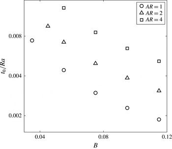
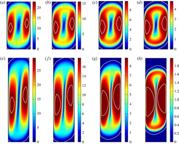
1. Introduction
We explore the hydrodynamic feasibility of a new type of heat transfer switch, able to reversibly govern the balance between conductive and convective heat transfer across a fluid filled cavity separating a hot and cold ambient. The key characteristic that we use here is that the activated fluid displays yield stress characteristics, whereas when not activated only viscous behaviour is observed. It is assumed that the change in the rheology happens quickly, is reversible and disappears once the fluid is deactivated.
Activating the fluid results in an increase in effective kinematic viscosity given by
 $$\begin{eqnarray}\displaystyle \hat{{\it\nu}}_{e}=\hat{{\it\nu}}+\frac{\hat{{\it\tau}}_{y}}{\hat{{\it\rho}}\hat{\dot{{\it\gamma}}}}, & & \displaystyle\end{eqnarray}$$
where
 $\hat{{\it\nu}}$
and
 $\hat{{\it\rho}}$
are the kinematic viscosity and density of the deactivated fluid and
 $\hat{{\it\tau}}_{y}$
is the yield stress due to the imposed activation. The rate of strain is denoted by
 $\hat{\dot{{\it\gamma}}}$
. An increase in the effective viscosity results in a decrease of effective Rayleigh number,
 $\mathit{Ra}_{e}$
, and weaker advection:
 $$\begin{eqnarray}\mathit{Ra}_{e}=\frac{{\hat{g}}\hat{{\it\beta}}{\rm\Delta}\hat{T}\hat{L}^{3}}{\hat{{\it\nu}}_{e}\hat{{\it\kappa}}}=\mathit{Ra}\frac{\hat{{\it\nu}}}{\hat{{\it\nu}}_{e}}.\end{eqnarray}$$
Here
 $\mathit{Ra}$
represents the nominal value of the Rayleigh number,
 ${\hat{g}}$
is the acceleration due to gravity,
 ${\rm\Delta}\hat{T}$
and
 $\hat{L}$
are the characteristic temperature difference and length scale of the domain,
 $\hat{{\it\beta}}$
and
 $\hat{{\it\kappa}}$
represent the coefficient of thermal expansion and thermal diffusivity of the fluid. In this paper we will denote dimensional quantities with the
 $\hat{\cdot }$
symbol and dimensionless quantities without.
At one extreme when the fluid is not activated,
 $\mathit{Ra}_{e}=\mathit{Ra}$
and heat transfer is similar to that of a Newtonian fluid, governed by a mix of conduction and advection. At the other extreme, when the activation is sufficiently strong, a high enough yield stress is developed such that the flow is suppressed everywhere:
 $\mathit{Ra}_{e}=0$
and heat transfer occurs only via conduction. The purpose of this work is to study the hydrodynamics of the convective flow and particularly the effect of the yield stress on transition characteristics between the conductive and convective limits.
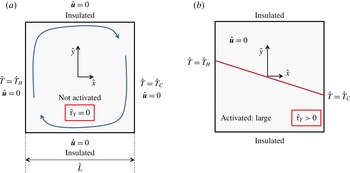
Square cavity filled with a smart viscoplastic fluid separates hot and cold walls: (a) deactivated state with no yield stress and convective internal flow; (b) sufficiently activated state with large yield stress, no fluid motion and conductive heat transfer only.

Natural convection of Newtonian fluids in a rectangular cavity has been studied extensively under a variety of boundary conditions (see e.g. Bejan Reference Bejan2004, chap. 5) for a review. In contrast, internal natural convection of viscoplastic fluids has been studied mostly within the last few decades. A number of studies derive analytical solutions for one-dimensional flows (Yang & Yeh Reference Yang and Yeh1965; Gershuni & Zhukhovitski Reference Gershuni and Zhukhovitski1973; Cherkasov Reference Cherkasov1979; Patel & Ingham Reference Patel and Ingham1994; Bayazitoglu, Paslay & Cernocky Reference Bayazitoglu, Paslay and Cernocky2007; Karimfazli & Frigaard Reference Karimfazli and Frigaard2013). Other more computational studies have focused on investigating the effect of the yield stress on steady-state heat-transfer characteristics; see Lyubimova (Reference Lyubimova1977), Vikhansky (Reference Vikhansky2009), Turan, Chakraborty & Poole (Reference Turan, Chakraborty and Poole2010) and Turan, Poole & Chakraborty (Reference Turan, Poole and Chakraborty2011). Finally, a few studies have considered flows for which a limiting value of the yield stress results in a static regime (e.g. Vikhansky Reference Vikhansky2010a ,Reference Vikhansky b ; Karimfazli & Frigaard Reference Karimfazli and Frigaard2013; Huilgol & Kefayati Reference Huilgol and Kefayati2015). It is these static regimes that have importance in the current study as being purely conductive.
There appears to be no study of the effect of a yield stress on the characteristics of a flow in transition between conductive and convective states, hence the focus of this paper. We thus make some idealizations and simplifications in dealing with rheology in order to investigate the problem at a more fundamental level. This allows us the use of analytical and numerical techniques and to draw conclusions that should be qualitatively applicable to a variety of different smart viscoplastic fluids. We use the simplest possible rheological model, the Bingham fluid, to describe the rheology of the activated smart fluid. Once deactivated the fluid is assumed to be Newtonian. This implies neglecting rheological processes happening on the activation timescale of the fluid. Our simplifying assumptions therefore amount to considering that the fluid remains isotropic and homogeneous with yield stress changing instantaneously under the application of a control (e.g. an electric field).
From a hydrodynamic perspective, the feasibility of the proposed idea depends not only on the existence of a static regime at sufficiently high yield stress, but also on both the stability of the static regime and on the transition times between conductive and convective flows. The maximum heat transfer across the cavity is determined by the steady-state Newtonian regime. The overall heat transfer, characterized by the mean Nusselt number
 $\overline{\mathit{Nu}}$
, varies with the aspect ratio,
 $h$
. This variation is more pronounced at higher values of Rayleigh number. Nonetheless, the global maximum is found at about
 $h=1$
(see Turan et al.
Reference Turan, Poole and Chakraborty2011 and the references therein). Hence, the convective heat transfer between two vertical plates at different temperatures can be enhanced by partitioning the space between the plates to smaller cells with
 $h\approx 1$
. We therefore focus our analysis on a square cavity; see figure 1.
Turan et al. (Reference Turan, Chakraborty and Poole2010, Reference Turan, Poole and Chakraborty2011) have utilized the regularized biviscosity model available in FLUENT to study the variation of heat transfer with the aspect ratio
 $h$
and other dimensionless groups. Huilgol & Kefayati (Reference Huilgol and Kefayati2015) recently studied the same problem in a square cavity using operator splitting methods with no regularization. Although the above-mentioned works use similar dimensionless formulations, we have chosen to use a different set of dimensionless parameters. Inevitably, this affects the role of certain dimensionless groups in the analysis. For completeness and to avoid confusion between parameter values in different formulations we briefly consider the steady-state regimes in appendix B.
There have been relatively few studies of the stability of naturally convecting viscoplastic fluids. Zhang, Vola & Frigaard (Reference Zhang, Vola and Frigaard2006) examined the Rayleigh–Bénard problem for a Bingham fluid using an energy method. They showed that for a finite yield stress this flow is linearly stable at all Rayleigh numbers (
 $\mathit{Ra}$
), is unconditionally energy stable for
 $\mathit{Ra}$
below the stability limit of the analogous Newtonian problem, and is conditionally stable otherwise. When stable, the kinetic energy of the perturbation decays to zero within a finite time. This finite stopping time behaviour is commonplace in studying the stability of the static state of yield stress fluids; the analysis originating with Glowinski and co-workers (Glowinski, Lions & Trémolières Reference Glowinski, Lions and Trémolières1981). Important from our perspective is that the stopping timescale is governed by the magnitude of the yield stress. Thus, we shall extend this analysis to the cavity flow studied here.
Other authors have studied the stability of convective viscoplastic flows from a more conventional linear and weakly nonlinear perspective. For example, Balmforth & Rust (Reference Balmforth and Rust2009) study the Rayleigh–Bénard problem in the limit of small Bingham number. Metivier and co-workers have extensively studied the Rayleigh–Bénard–Poiseuille flow along a plane channel (Métivier & Nouar Reference Métivier and Nouar2008, Reference Métivier and Nouar2009; Métivier, Nouar & Brancher Reference Métivier, Nouar and Brancher2010; Métivier & Magnin Reference Métivier and Magnin2011). Although interesting, these approaches are less relevant for flow control. Finally, a number of authors have recently studied the onset of natural convection experimentally using solutions of Carbopol (e.g. Darbouli et al. Reference Darbouli, Métivier, Piau, Magnin and Abdelali2013; Davaille et al. Reference Davaille, Gueslin, Massmeyer and DiGiuseppe2013; Kebiche, Castelain & Burghelea Reference Kebiche, Castelain and Burghelea2014).
An outline of our paper is as follows. The problem is formulated in § 2 and the computational method is also outlined. In § 3 we demonstrate that for a sufficiently large yield stress the steady state is motionless. Variational and numerical techniques are used to estimate the limits of yielding. In § 3.2 we extend the approach of Zhang et al. (Reference Zhang, Vola and Frigaard2006) to our configuration. Where the analysis differs is that the base conductive Newtonian state is linearly unstable at all
 $\mathit{Ra}$
. Thus, we have to first consider sufficiently large
 $B$
, in order to ensure a static steady state. We also extend the analysis of Joseph (Reference Joseph1965) to provide bounds on the
 $\mathit{Ra}$
that ensure the unconditional stability of the static regime (i.e. assuming sufficiently large
 $B$
). The transition between Newtonian and viscoplastic steady states is studied in § 4, giving estimates for the different timescales. In § 5 we explore the effects of varying the Prandtl number. Finally, the paper concludes in § 6 by considering the relative dimensional parameters required for application of this methodology. We point out also some areas where, although the methodology works, improvements could be made.
2. Problem set-up
2.1. Formulation
We consider a fluid-filled square cavity of width
 $\hat{L}$
with differentially heated side walls, maintained at temperatures
 $\hat{T}_{H}$
and
 $\hat{T}_{C}$
, with temperature difference
 ${\rm\Delta}\hat{T}=\hat{T}_{H}-\hat{T}_{C}>0$
; see figure 1. We consider the fluid to be a smart viscoplastic fluid and are concerned only with simple situations in which the fluid is either uniformly activated, or not activated at all. Assuming the response time of the fluid is much faster than that of other hydrodynamic timescales, we make the simple assumption that the fluid may be switched (rheologically) between a yield stress fluid and a purely viscous fluid, instantaneously: when activated the fluid is assumed to behave rheologically as a Bingham fluid, with yield stress
 $\hat{{\it\tau}}_{y}$
and plastic viscosity
 $\hat{{\it\mu}}$
, and as a Newtonian fluid otherwise (i.e.
 $\hat{{\it\tau}}_{y}=0$
). For simplicity we ignore possible changes in
 $\hat{{\it\mu}}$
.
Flow is promoted by buoyancy forces resulting from the temperature gradient between the two vertical walls. This is governed by the momentum, the continuity and the energy equations. Assuming the Boussinesq approximation, these equations are expressed in dimensionless form as
 $$\begin{eqnarray}\displaystyle & \displaystyle \frac{\mathit{Ra}}{\mathit{Pr}}\;\frac{\partial u_{i}}{\partial t}+\frac{\mathit{Ra}}{\mathit{Pr}}\;u_{j}\frac{\partial u_{i}}{\partial x_{j}}=-\frac{\partial p}{\partial x_{i}}+\frac{\partial {\it\tau}_{ij}}{\partial x_{j}}+T{\it\delta}_{i2}, & \displaystyle\end{eqnarray}$$
 $$\begin{eqnarray}\displaystyle & \displaystyle \frac{\partial u_{i}}{\partial x_{i}}=0, & \displaystyle\end{eqnarray}$$
 $$\begin{eqnarray}\displaystyle & \displaystyle \mathit{Ra}\frac{\partial T}{\partial t}+\mathit{Ra}\;u_{i}\frac{\partial T}{\partial x_{i}}=\frac{\partial ^{2}T}{\partial x_{i}\partial x_{i}}, & \displaystyle\end{eqnarray}$$
 $$\begin{eqnarray}\left.\begin{array}{@{}cc@{}}\displaystyle {\it\tau}_{ij}=\left(1+\frac{B}{\dot{{\it\gamma}}}\right)\dot{{\it\gamma}}_{ij} & \text{iff }{\it\tau}>B\\ \dot{{\it\gamma}}=0 & \text{iff }{\it\tau}\leqslant B\end{array}\right\}\end{eqnarray}$$
where
 $$\begin{eqnarray}{\it\tau}=\sqrt{\frac{1}{2}{\it\tau}_{ij}{\it\tau}_{ij}},\quad \dot{{\it\gamma}}=\sqrt{\frac{1}{2}\dot{{\it\gamma}}_{ij}\dot{{\it\gamma}}_{ij}},\quad \dot{{\it\gamma}}_{ij}=\frac{\partial u_{i}}{\partial x_{j}}+\frac{\partial u_{j}}{\partial x_{i}}.\end{eqnarray}$$
Boundary conditions at the side walls are
 $$\begin{eqnarray}\displaystyle & \displaystyle u_{i}(\pm 1/2,y)=0, & \displaystyle\end{eqnarray}$$
 $$\begin{eqnarray}\displaystyle & \displaystyle T(\pm 1/2,y)=\mp 1/2 & \displaystyle\end{eqnarray}$$
 $y=\pm 1/2$
 $$\begin{eqnarray}\displaystyle & \displaystyle u_{i}(x,\pm 1/2)=0, & \displaystyle\end{eqnarray}$$
 $$\begin{eqnarray}\displaystyle & \displaystyle \frac{\partial T}{\partial y}(x,\pm 1/2)=0. & \displaystyle\end{eqnarray}$$
All lengths have been scaled with
 $\hat{L}$
, stresses with
 $\hat{{\it\tau}}^{\ast }=\hat{{\it\rho}}_{0}{\hat{g}}\hat{{\it\beta}}{\rm\Delta}\hat{T}\hat{L}$
and velocity with a velocity scale
 $\hat{V}^{\ast }$
that balances viscous and buoyancy forces:
 $\hat{V}^{\ast }=\hat{{\it\tau}}^{\ast }\hat{L}/\hat{{\it\mu}}$
. The density
 $\hat{{\it\rho}}_{0}$
is evaluated at a reference temperature
 $T_{0}=(\hat{T}_{C}+\hat{T}_{H})/2$
. Thus, dimensionless variables are
 $$\begin{eqnarray}\displaystyle \left.\begin{array}{@{}c@{}}\displaystyle x_{i}=\frac{\hat{x_{i}}}{\hat{L}},\quad T=\frac{\hat{T}-\hat{T}_{0}}{\hat{T}_{H}-\hat{T}_{C}},\quad u_{i}=\frac{\hat{{\it\nu}}\,\hat{u_{i}}}{{\hat{g}}\hat{{\it\beta}}{\rm\Delta}\hat{T}\hat{L}^{2}},\\ \displaystyle P=\frac{\hat{P}}{\hat{{\it\rho}}_{0}{\hat{g}}\hat{{\it\beta}}{\rm\Delta}\hat{T}\hat{L}},\quad t=\frac{{\hat{g}}\hat{{\it\beta}}{\rm\Delta}\hat{T}\hat{L}\hat{t}}{\hat{{\it\nu}}},\quad {\it\tau}_{ij}=\frac{\hat{{\it\tau}}_{ij}}{\hat{{\it\rho}}_{0}{\hat{g}}\hat{{\it\beta}}{\rm\Delta}\hat{T}\hat{L}}.\end{array}\right\} & & \displaystyle\end{eqnarray}$$
The dimensionless groups governing this problem are the Rayleigh number,
 $\mathit{Ra}$
(alternatively the Grashof number,
 $\mathit{Gr}$
), Prandtl number,
 $\mathit{Pr}$
, the aspect ratio and a Bingham number (sometimes called yield number or Oldroyd number),
 $B$
:
 $$\begin{eqnarray}\mathit{Ra}=\frac{{\hat{g}}\hat{{\it\beta}}{\rm\Delta}\hat{T}\hat{L}^{3}}{\hat{{\it\nu}}\hat{{\it\kappa}}}=\mathit{Gr}\,\mathit{Pr},\quad \mathit{Pr}=\frac{\hat{{\it\nu}}}{\hat{{\it\kappa}}},\quad B=\frac{\hat{{\it\tau}}_{y}}{\hat{{\it\rho}}_{0}{\hat{g}}\hat{{\it\beta}}{\rm\Delta}\hat{T}\hat{L}}.\end{eqnarray}$$
In terms of heat transfer, note that the conductive limit of this problem is simply
 $T=-x$
and we measure the effectiveness of heat transfer across the cavity via the Nusselt number,
 $\mathit{Nu}_{\pm }$
, computed from the solution along each sidewall as:
 $$\begin{eqnarray}\mathit{Nu}_{\pm }=-\frac{\partial T}{\partial x}(\pm 1/2,y).\end{eqnarray}$$
To give a single measure of heat transfer, we will average the Nusselt number over both sidewalls (
 $\overline{\mathit{Nu}}$
) and/or consider the maximum (
 $\mathit{Nu}_{\mathit{max}}$
). Denoting
 ${\it\theta}$
by
 $T=-x+{\it\theta}$
, we can see that
 $$\begin{eqnarray}\mathit{Nu}_{\pm }=1-\frac{\partial {\it\theta}}{\partial x}(\pm 1/2,y).\end{eqnarray}$$
Hence,
 $\overline{\mathit{Nu}}-1$
represents the average convective contribution to heat transfer, induced by buoyancy and computed from
 ${\it\theta}$
.
2.2. Computational method
The governing equations (2.1)–(2.3) with corresponding boundary conditions are solved using an augmented Lagrangian algorithm combined with a finite volume/staggered grid space discretization. The numerical strategy employed here is very similar to that in Vinay, Wachs & Agassant (Reference Vinay, Wachs and Agassant2005), except that in this work the momentum and energy equations are two-way coupled by the buoyancy term and the problem is posed in a planar geometry instead of an axisymmetric one.
At the mathematical level, adopting the constitutive equation of a Bingham fluid gives rise to two specific properties: (i) the stress field is undetermined when the stain-rate field is zero; and (ii) the equation is non-differentiable at the yield point. Two classical families of numerical methods have been suggested to circumvent these issues. The first is the well-known regularization method, which approximates the true yield stress law with a continuous function with bounded effective viscosity. This transforms the problem into a generalized Newtonian problem in which the material is treated as highly viscous in regions where it is supposed not to yield. At the computational level, classical solution methods for shear-thinning/shear-thickening fluid flows are used. Although practical, this technique raises issues in terms of the determination of the yield surface and also prevents one from properly simulating finite time decay of the kinetic energy, a property that is deemed to be essential in our study. This defect is simply because generalized Newtonian (i.e. purely viscous) materials do not return to rest in finite time, even if their viscosity is very high. The second method relies on the use of Lagrange multiplier and decomposition–coordination algorithm and is referred to in the literature as an augmented Lagrangian algorithm. It has been shown that, when combined with a fully implicit backward Euler time discretization, this algorithm computes return to rest in finite time in an accurate way (in the sense that at rest the strain-rate field is computationally zero everywhere in the flow domain). This is because the original form of the Bingham constitutive equation is considered. For an extended discussion on regularization techniques and the augmented Lagrangian algorithm, the interested reader is referred to Frigaard & Nouar (Reference Frigaard and Nouar2005) and Glowinski & Wachs (Reference Glowinski and Wachs2011), respectively.
The coupling between the momentum and energy equations via the buoyancy term is accounted for in a weak way, which implies that at each time step the temperature field of the previous time is used to compute
 $T{\it\delta}_{i2}$
in (2.1). For both the momentum and energy equations, the diffusion terms (viscous and plastic stress, and conduction respectively) are discretized first-order fully implicitly in time and second order in space, with a centred scheme. The advection terms are treated first-order explicitly in time and discretized in space with a second-order total variation diminishing scheme. Overall, the solution algorithm is first-order accurate in time. The explicit treatment of the advection term in the momentum equation does not prevent return to rest in a finite time, since as the fluid becomes close to rest the advection term becomes negligible and the flow is of Stokes type. A more detailed presentation of the numerical algorithm is presented in appendix A.
All simulations are performed with PeliGRIFF, a code that has been developed for numerical computation of two phase flows (e.g. particles, drops or bubbles suspended in Newtonian or yield stress fluids); see Rahmani & Wachs (Reference Rahmani and Wachs2014) for more details.
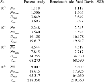
To verify the accuracy of our computational code, we have first compared against the Newtonian benchmark results of de Vahl Davis (Reference de Vahl Davis1983), who give average and maximal Nusselt numbers as well as the maximal velocity components, for
 $\mathit{Pr}=0.71$
. The results agree well with the benchmark data; see table 1. Examples of the Newtonian solution are given later in figures 15(a–c) and 16(a–c).
Comparison with the Newtonian benchmark computed by de Vahl Davis (Reference de Vahl Davis1983), at
 $\mathit{Pr}=0.71$
.

A similar comparison is made by Turan et al. (Reference Turan, Chakraborty and Poole2010), who have computed the flow of a Bingham fluid in a heated cavity. Thus, we also benchmark our results against those of Turan et al. (Reference Turan, Chakraborty and Poole2010) (for their parameters
 $\mathit{Bn}=0.5$
,
 $\mathit{Ra}=10^{4}$
and
 $\mathit{Pr}=7$
), over a range of uniform mesh sizes; see table 2. Note in this comparison that the dimensionless parameters in our study are defined differently to those of Turan et al. (Reference Turan, Chakraborty and Poole2010), but related by a simple algebraic transformation. The agreement is again satisfactory. Indeed Turan et al. (Reference Turan, Chakraborty and Poole2010) use a form of Richardson extrapolation to achieve higher accuracy at lower mesh resolution, whereas it appears that our computations show better mesh convergence (at least for the parameters used in this case).
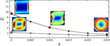
Effect of
 $\mathit{Ra}$
,
 $B$
and
 $\mathit{Pr}$
on
 $\overline{\mathit{Nu}}$
. Empty and filled markers represent
 $\mathit{Ra}=10^{4}$
and
 $10^{6}$
, respectively. Results are presented at
 $\mathit{Pr}=1$
(▫),
 $\mathit{Pr}=10$
(◃) and
 $\mathit{Pr}=100$
(▹). Note that at each
 $\mathit{Ra}$
different symbols overlap and are thus not discernible. The insets are colourmaps of
 $|\boldsymbol{u}|$
scaled such that for each inset
 $\max (|\boldsymbol{u}|)=1$
. White curves represent the yield surfaces. Red circular symbols (○) mark the points for which the colourmap of velocity is provided.

Comparison with Turan et al. (Reference Turan, Chakraborty and Poole2010), table 2, for
 $\mathit{Bn}=({\it\tau}_{y}/{\it\mu})\sqrt{L/(g{\it\beta}{\rm\Delta}T)}=0.5$
,
 $\mathit{Ra}=10^{4}$
,
 $\mathit{Pr}=7$
. The mesh sizes are
 $\text{M}2=40\times 40$
,
 $\text{M}3=80\times 80$
,
 $\text{M}4=160\times 160$
.

Third, we tried to reproduce the results presented by Vola, Boscardin & Latché (Reference Vola, Boscardin and Latché2003) but were unable to do so. We believe that this difficulty is mainly a problem with interpreting the dimensional and dimensionless parameters used by Vola et al. (Reference Vola, Boscardin and Latché2003), which are incompletely specified.
2.3. Overview of the steady regime
Before proceeding with our study, we outline the main characteristics of the steady-state flow. This has been studied extensively e.g. by Turan et al. (Reference Turan, Chakraborty and Poole2010). We present an overview of steady regimes and clarify the variation of features of steady regimes with
 $\mathit{Ra}$
,
 $\mathit{Pr}$
and
 $B$
. Figure 2 illustrates the variation in steady state
 $\overline{\mathit{Nu}}$
at
 $\mathit{Ra}=10^{4},10^{6}$
for a wide range of
 $B$
, computed for three values of
 $\mathit{Pr}=1,~10,~100$
. At a critical
 $B=B_{cr}$
(studied below in § 3) the flows become static. Values of
 $B<B_{cr}$
have been chosen for figure 2 so that the steady states are convective.
As
 $B$
increases we observe a monotone decrease in heat transfer, captured by
 $\overline{Nu}$
. When
 $B<B_{cr}$
, buoyant stresses are only partly balanced by the yield stress. What remains of the buoyant stresses drives the flow and, depending on the value of other dimensionless parameters, is balanced by advection or diffusion of momentum. As
 $B$
is increased from zero to the critical limit,
 $\mathit{Ra}_{e}$
decreases. A larger fraction of the buoyancy stresses is balanced by the yield stress, advective heat transfer becomes weaker and
 $\overline{\mathit{Nu}}$
decreases.
A few colourmaps of the velocity magnitude are inset into figure 2 to illustrate the different characteristic regimes. As
 $\mathit{Ra}$
increases, heat transfer due to advection dominates diffusive heat transfer. This results in a noticeable deviation of the temperature field from the purely conductive regime and formation of boundary layers on the vertical cavity walls, enhancing heat transfer. As
 $B$
increases we observe growing regions of unyielded fluid, which suppresses advective heat transfer. A more detailed illustration of the flow features at different
 $\mathit{Ra}$
and
 $B$
is provided for reference in appendix B.
The most obvious feature noticeable in figure 2 is a relative insensitivity of
 $\overline{\mathit{Nu}}$
to
 $\mathit{Pr}$
. Note that only
 $\mathit{Pr}\geqslant 1$
is considered, as is very common for yield stress fluids. This insensitivity may be explained as follows. Assuming that advection and diffusion of thermal energy are balanced and using continuity, we find that the characteristic dimensionless velocity in direction
 $i$
,
 $U_{i}$
, scales as
 $$\begin{eqnarray}U_{i}\sim \frac{{\it\Theta}l_{i}}{\mathit{Ra}\min (l_{i})^{2}},\end{eqnarray}$$
where
 $l_{i}$
is the characteristic dimensionless length scale of gradients in the
 $x_{i}$
direction. Here
 ${\it\Theta}$
is a measure of the deviation of the dimensionless temperature field from the (linear) conductive regime. Using this characteristic velocity, diffusive and advective terms in the vertical momentum balance scale as follows:
 $$\begin{eqnarray}\displaystyle & \displaystyle \frac{\partial ^{2}u_{2}}{\partial x_{i}\partial x_{i}}\sim \frac{U_{2}}{\min (l_{i})^{2}}=\frac{{\it\Theta}l_{2}}{\mathit{Ra}\,\min (l_{i})^{4}} & \displaystyle\end{eqnarray}$$
 $$\begin{eqnarray}\displaystyle & \displaystyle \frac{\mathit{Ra}}{\mathit{Pr}}u_{j}\frac{\partial u_{2}}{\partial x_{j}}\sim \frac{\mathit{Ra}\,U_{2}^{2}}{\mathit{Pr}\,l_{2}}=\frac{{\it\Theta}^{2}l_{2}}{\mathit{Ra}\,\mathit{Pr}\,\min (l_{i})^{4}}. & \displaystyle\end{eqnarray}$$
 ${\it\Theta}$
and
 $l_{i}$
vary with
 $\mathit{Ra}$
and
 $B$
, it can be observed that for all values of
 $\mathit{Ra}$
the ratio between diffusive and advective momentum transfer is
 $\mathit{Pr}/{\it\Theta}$
. Here
 ${\it\Theta}$
is generally small, particularly at low
 $\mathit{Ra}_{e}$
, and decreases as
 $\mathit{Ra}_{e}\rightarrow \infty$
.
Therefore, when
 $\mathit{Pr}/{\it\Theta}\gg 1$
, advection of momentum is negligible in comparison with the diffusion of momentum. Thus, viscous diffusion together with the yield stress balance buoyancy. Assuming this dominance of viscous diffusion over advection of momentum, all of the terms involving
 $\mathit{Pr}$
in the governing equations (2.1)–(2.3) are small, except the time derivatives. This explains why the effect of
 $\mathit{Pr}\geqslant 1$
on steady-state characteristics appears negligible.
3. The conductive limit
We now consider the motionless limit of the steady flow solution, i.e.
 $\boldsymbol{u}=0$
, that we expect to exist if the yield stress is large enough. The temperature evolves over a timescale
 $t\sim \mathit{Ra}$
, to attain a steady state:
 $$\begin{eqnarray}\frac{\partial T}{\partial x_{i}\partial x_{i}}=0,\end{eqnarray}$$
with solution
 $T=-x$
satisfying the boundary conditions. This temperature field provides a steady buoyancy force:
 $$\begin{eqnarray}0=-\frac{\partial p}{\partial x_{i}}+\frac{\partial {\it\tau}_{ij}}{\partial x_{j}}-x{\it\delta}_{i2}.\end{eqnarray}$$
We observe that (3.2) governs the statically admissible stress fields possible with the conductive buoyancy force. If there is an admissible stress field with
 ${\it\tau}\leqslant B$
, then a static solution is possible. Note that the statically admissible stress fields are governed only by the domain geometry and boundary conditions, being completely independent of
 $\mathit{Ra}$
and
 $\mathit{Pr}$
. The smallest value
 $B$
for which there is a static solution is the critical Bingham number, say
 $B_{cr}$
, which is therefore also independent of
 $\mathit{Ra}$
and
 $\mathit{Pr}$
.
This may indeed be intuitive since when the velocity is zero everywhere in the domain, the temperature profile and the buoyancy forces are independent of the rates at which momentum and heat diffuse. Yielding starts when buoyancy forces dominate yield stress. Thus, a comparison of the two magnitudes, represented in the Bingham number
 $B$
, is natural in determining the start of yielding. It is the actual distribution of buoyancy forces that determine the value of
 $B_{cr}$
. This argument is quite general: the shape of the domain will influence the conductive temperature distribution and the computation of admissible stress fields. However,
 $B_{cr}$
will remain independent of
 $\mathit{Ra}$
and
 $\mathit{Pr}$
.
3.1. Critical Bingham number
The conductive limit is itself a steady-state solution of (2.1)–(2.9). Analysis of the steady-state problem provides an alternative way to define the critical Bingham number, by examining changes in the steady state as
 $B$
is increased. We write again
 $T={\it\theta}-x$
, so that
 ${\it\theta}$
denotes the non-conductive part of the temperature field. Starting with the energy and momentum equations, we set the time derivatives to zero. On multiplying the energy equation by
 ${\it\theta}$
and integrating over the domain we get
 $$\begin{eqnarray}-\mathit{Ra}\langle u_{1}{\it\theta}\rangle +\left\langle \frac{\partial {\it\theta}}{\partial x_{i}}\frac{\partial {\it\theta}}{\partial x_{i}}\right\rangle =0,\end{eqnarray}$$
where
 $$\begin{eqnarray}\langle \,f\rangle =\int _{{\it\Omega}}f\,\text{d}x.\end{eqnarray}$$
From the Cauchy–Schwarz inequality
 $$\begin{eqnarray}\langle u_{1}{\it\theta}\rangle \leqslant \Vert u_{1}\Vert \,\Vert {\it\theta}\Vert ,\end{eqnarray}$$
and using the Poincaré inequality we have
 $$\begin{eqnarray}\tilde{C}_{p}\Vert {\it\theta}\Vert ^{2}\leqslant \left\langle \frac{\partial {\it\theta}}{\partial x_{i}}\frac{\partial {\it\theta}}{\partial x_{i}}\right\rangle ,\end{eqnarray}$$
where for a square cavity we have
 $\tilde{C}_{p}=4{\rm\pi}^{2}$
. In this paper
 $\Vert \cdot \Vert$
will denote the
 $L^{2}$
norm. The above two inequalities together with (3.3) yield
 $$\begin{eqnarray}\tilde{C}_{p}\Vert {\it\theta}\Vert \leqslant \mathit{Ra}\Vert u_{1}\Vert .\end{eqnarray}$$
Similarly, multiplying the differential form of momentum equation by
 $u_{i}$
and integrating over the domain, we have
 $$\begin{eqnarray}\langle \dot{{\it\gamma}}^{2}\rangle +B\langle \dot{{\it\gamma}}\rangle -\langle u_{2}({\it\theta}-x)\rangle =0.\end{eqnarray}$$
Assuming that
 $\langle \dot{{\it\gamma}}\rangle >0$
, on using (3.7) and the Cauchy–Schwarz inequality we find
 $$\begin{eqnarray}0\leqslant \langle \dot{{\it\gamma}}^{2}\rangle =-B\langle \dot{{\it\gamma}}\rangle +\langle u_{2}({\it\theta}-x)\rangle 0\leqslant -\langle \dot{{\it\gamma}}\rangle \left[B-\frac{Ra}{\tilde{C}_{p}}\frac{\Vert u_{1}\Vert \,\Vert u_{2}\Vert }{\langle \dot{{\it\gamma}}\rangle }+\frac{\langle u_{2}x\rangle }{\langle \dot{{\it\gamma}}\rangle }\right].\end{eqnarray}$$
Owing to the boundary conditions, unless
 $\boldsymbol{u}=0$
, the velocity
 $\boldsymbol{u}$
does not represent a rigid–body motion. For such
 $\boldsymbol{u}\neq 0$
, it is shown by Temam & Strang (Reference Temam and Strang1980) that there exists a constant
 $C_{TS}>0$
such that
 $$\begin{eqnarray}C_{TS}\Vert \boldsymbol{u}\Vert \leqslant \langle \dot{{\it\gamma}}\rangle .\end{eqnarray}$$
Thus, the last term in (3.9) is bounded above, i.e.
 $$\begin{eqnarray}-\frac{\langle u_{2}x\rangle }{\langle \dot{{\it\gamma}}\rangle }\leqslant \frac{\Vert u_{2}\Vert \,\Vert x\Vert }{\langle \dot{{\it\gamma}}\rangle }\leqslant \frac{\Vert x\Vert }{C_{TS}}.\end{eqnarray}$$
It follows that the second term in (3.9) is also bounded as follows:
 $$\begin{eqnarray}\frac{\mathit{Ra}}{\tilde{C}_{p}}\frac{\Vert u_{2}\Vert \,\Vert u_{1}\Vert }{\langle \dot{{\it\gamma}}\rangle }\leqslant \frac{\mathit{Ra}}{\tilde{C}_{p}C_{TS}}\Vert \boldsymbol{u}\Vert .\end{eqnarray}$$
Let us assume that
 $\Vert \boldsymbol{u}\Vert$
is bounded above for all
 $B$
,
 $\mathit{Pr}$
and
 $\mathit{Ra}$
of interest, as is anyway expected physically. Then we may take
 $B$
sufficiently large that the right-hand side of (3.9) is strictly negative. Thus, the assumption that
 $\langle \dot{{\it\gamma}}\rangle >0$
is contradicted and it follows that
 $\boldsymbol{u}=0$
.
This establishes that, provided
 $\Vert \boldsymbol{u}\Vert$
is bounded (or indeed grows slower than linear in
 $B$
), there exists a
 $B$
above which
 $\boldsymbol{u}=0$
. Of course normally, as we have seen, we would expect that
 $\Vert \boldsymbol{u}\Vert$
decreases with
 $B$
. Suppose therefore that
 $B_{cr}$
is the smallest
 $B$
for which
 $\boldsymbol{u}=0$
for all
 $B>B_{cr}$
, and let us assume that
 $\Vert \boldsymbol{u}\Vert$
varies continuously with
 $B$
, with say
 $\Vert \boldsymbol{u}\Vert \sim |B_{cr}-B|^{{\it\delta}}$
as
 $B\rightarrow B_{cr}^{-}$
for some
 ${\it\delta}>0$
. It follows that the second term of (3.9) approaches zero faster than the third term, by a factor of
 $|B_{cr}-B|^{{\it\delta}}$
. Thus, as
 $B\rightarrow B_{cr}^{-}$
the inequality (3.9) is dominated by
 $$\begin{eqnarray}0\leqslant \langle \dot{{\it\gamma}}^{2}\rangle \lesssim -\langle \dot{{\it\gamma}}\rangle \left[B+\frac{\langle u_{2}x\rangle }{\langle \dot{{\it\gamma}}\rangle }\right].\end{eqnarray}$$
Now let
 $\mathscr{V}_{0}$
be the test space of divergence-free velocity fields with components in
 $H_{0}^{1}([-1/2,1/2]\times [-1/2,1/2])$
, then we have that
 $$\begin{eqnarray}-\frac{\langle u_{2}x\rangle }{\langle \dot{{\it\gamma}}(\boldsymbol{u})\rangle }\leqslant \sup _{\boldsymbol{v}\in \mathscr{V}_{0},\boldsymbol{v}\not =0}\left\{-\frac{\langle v_{2}x\rangle }{\langle \dot{{\it\gamma}}(\boldsymbol{v})\rangle }\right\}.\end{eqnarray}$$
If we define
 $B_{cr}$
in the following way:
 $$\begin{eqnarray}B_{cr}=\sup _{\boldsymbol{v}\in \mathscr{V}_{0},\boldsymbol{v}\not =0}\left\{-\frac{\langle v_{2}x\rangle }{\langle \dot{{\it\gamma}}(\boldsymbol{v})\rangle }\right\},\end{eqnarray}$$
then under the assumption that
 $\Vert \boldsymbol{u}\Vert \rightarrow 0$
continuously as
 $B\rightarrow B_{cr}^{-}$
, we have that
 $\boldsymbol{u}=0$
if
 $B\geqslant B_{cr}$
.
Let us observe that
 $B_{cr}$
defined by (3.15) is strictly an upper estimate for the critical Bingham number, derived from general functional properties. In order for the bound to be sharp it is necessary for the solution
 $\boldsymbol{u}$
to be a maximizer of (3.15). To examine this, it is helpful to consider the variational form of the steady-state problem. The steady-state solution is equivalent to finding the (admissible) pair
 $({\it\theta},\boldsymbol{u})$
that minimizes
 $$\begin{eqnarray}\displaystyle & \displaystyle \mathscr{K}({\it\varphi},\boldsymbol{v})=\frac{1}{2}\left\langle \frac{\partial {\it\varphi}}{\partial x_{i}}\frac{\partial {\it\varphi}}{\partial x_{i}}\right\rangle -Ra\langle v_{1}{\it\varphi}\rangle , & \displaystyle\end{eqnarray}$$
 $$\begin{eqnarray}\displaystyle & \displaystyle \mathscr{J}({\it\varphi},\boldsymbol{v})={\textstyle \frac{1}{2}}\langle \dot{{\it\gamma}}(\boldsymbol{v})^{2}\rangle +B\langle \dot{{\it\gamma}}(\boldsymbol{v})\rangle -\langle v_{2}({\it\varphi}-x)\rangle , & \displaystyle\end{eqnarray}$$
 $\Vert \boldsymbol{u}\Vert \sim |B_{cr}-B|^{{\it\delta}}$
as
 $B\rightarrow B_{cr}^{-}$
, from the first of these we can see that
 $\Vert {\it\theta}\Vert \sim |B_{cr}-B|^{{\it\delta}}$
as
 $B\rightarrow B_{cr}^{-}$
, e.g. following (3.7), or noting that
 $u_{2}$
provides the data for the
 ${\it\varphi}$
minimization. Therefore close to
 $B_{cr}$
we see that
 $$\begin{eqnarray}\mathscr{J}({\it\varphi},\boldsymbol{v})\sim O(|B_{cr}-B|^{2{\it\delta}})+B\langle \dot{{\it\gamma}}(\boldsymbol{v})\rangle +O(|B_{cr}-B|^{2{\it\delta}})+\langle v_{2}x\rangle ,\end{eqnarray}$$
with the leading-order terms of order
 $|B_{cr}-B|^{{\it\delta}}$
. We see that the minimizer of the leading-order problem is indeed a maximizer of (3.15), which leads us to believe that
 $B_{cr}$
defined by (3.15) is sharp. The above arguments need however to be made fully rigorous.
The computational results suggest that close to the critical limit, the fluid is yielded only in a very narrow ring of diameter of approximately one and width
 ${\it\varepsilon}$
. This suggests that the optimization problem (3.15) can be evaluated analytically for a square cavity. A function with the same approximate profile as the solution is the following:
 $$\begin{eqnarray}v_{{\it\theta}}=\left\{\begin{array}{@{}ll@{}}\displaystyle -r{\it\omega},\quad & \displaystyle r\leqslant \frac{1}{2}-{\it\varepsilon},\\ \displaystyle -\left(\frac{1}{2}-{\it\varepsilon}\right){\it\omega}\frac{1/2-r}{{\it\varepsilon}},\quad & \displaystyle \frac{1}{2}-{\it\varepsilon}\leqslant r\leqslant \frac{1}{2},\end{array}\right.\end{eqnarray}$$
with
 $v_{r}=0$
. Here
 $(r,{\it\theta})$
represent polar coordinates located at the centre of the square cavity:
 ${\it\omega}$
is the angular velocity of the unyielded region at the centre of the square. Evaluating (3.15) using the above profile gives
 $B_{cr}=1/32$
as
 ${\it\varepsilon}\rightarrow 0$
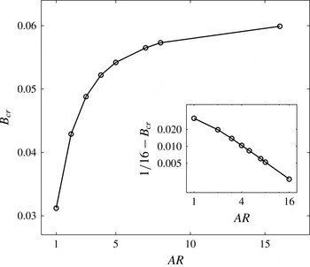
. The circular shape of the plug in a square cavity is exceptional in the configuration of plugs close to yielding (see appendix C). The symmetry of the square allows rigid–body rotation of a properly circular plug. However, for sufficiently larger (or smaller) values of the aspect ratio, we find four moving plug regions that are in rigid–body motion.
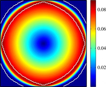
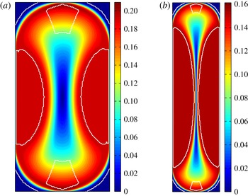
We can also estimate the value of critical Bingham number using our numerical solutions. Indeed a key point in using the augmented Lagrangian approach is that the method resolves zero strain rates, whereas a regularization method such as in Turan et al. (Reference Turan, Chakraborty and Poole2010, Reference Turan, Poole and Chakraborty2011) is not suitable for studying these limits. Figure 3 illustrates the velocity field and plug boundaries at Bingham numbers just smaller than
 $B_{cr}$
. The streamlines in the plug are circular, although the yield surfaces are not quite circular for the Bingham number presented here. To estimate
 $B_{cr}$
numerically we evaluated the steady-state solution at a number of different
 $B$
values close to
 $B_{cr}$
and computed the value of
 $\Vert \boldsymbol{u}\Vert$
. Then, for the three values of
 $B$
closest to stopping, we used a linear fit to find
 $B_{cr}$
by extrapolation. The numerical results found in this way compare well with the analytical results.
To summarize, analysis of the steady flows reveals that for sufficiently large
 $B$
the steady velocity solution
 $\boldsymbol{u}=0$
. The analysis allows a rigorous definition of the critical
 $B_{cr}$
, in terms of an optimization problem (3.15). As with our physical intuition,
 $B_{cr}$
depends only on the domain considered and steady conductive problem, but not on other parameters. Furthermore the actual solution minimizes (3.15) and this gives us a number of different ways of estimating
 $B_{cr}$
. Using these we find
 $B_{cr}=1/32$
for the square cavity. Different aspect ratios are considered in appendix C.
Colourmap of
 $\mathit{Ra}\Vert \boldsymbol{u}\Vert$
as
 $B\rightarrow B_{cr}^{-}$
, at
 $B=0.0311$
,
 $\mathit{Ra}=10^{5}$
,
 $\mathit{Pr}=1$
. The white curves represent yield surfaces.

3.2. Stability of the static regime
To summarize the previous results, we have seen that for sufficiently large yield stress
 $B>B_{cr}$
the steady-state solution is the static regime. In the context of our smart fluid application, if we apply a sufficiently strong activation signal (i.e. such that
 $B>B_{cr}$
), the static state is found. The question we now answer is whether or not the conductive static state is stable.
We assume throughout that
 $B>B_{cr}$
. The steady state is static and purely conductive. Thus, the temperature is given by
 $T=-x$
. The steady velocity is zero, but the stresses within the fluid need not be zero. Indeed, any combination of pressure
 $P$
and residual deviatoric stresses
 ${\it\tau}_{b,ij}$
is admissible if it satisfies the Stokes system:
 $$\begin{eqnarray}0=-\frac{\partial P}{\partial x_{i}}+\frac{\partial {\it\tau}_{b,ij}}{\partial x_{j}}-x{\it\delta}_{i2}.\end{eqnarray}$$
As we consider static regimes, we clearly also require that the residual stresses
 ${\it\tau}_{b,ij}$
satisfy
 $$\begin{eqnarray}{\it\tau}_{b}=\sqrt{{\textstyle \frac{1}{2}}{\it\tau}_{b,ij}{\it\tau}_{b,ij}}<B.\end{eqnarray}$$
Also, by the above reasoning we may assume that
 $\Vert {\it\tau}_{b}\Vert _{\infty }<B<\infty$
, where
 $\Vert {\it\tau}_{b}\Vert _{\infty }$
denotes the
 $L^{\infty }({\it\Omega})$
norm of
 ${\it\tau}_{b}$
, i.e. the supremum norm. Finally, as discussed by Zhang et al. (Reference Zhang, Vola and Frigaard2006), the static base state is linearly stable. This follows since a shear stress disturbance of a finite magnitude (at least
 $B-{\it\tau}_{b}$
) is needed to yield the fluid anywhere and initiate a flow.
We consider a perturbed solution
 $(u_{i},{\it\tau}_{b,ij}+{\it\tau}_{ij},P+p,T+{\it\theta})$
, that satisfies (2.1)–(2.3), as does the steady state
 $(0,{\it\tau}_{b,ij},P,T)$
. Subtracting the steady-state equations from the perturbed equations yields the perturbation equations:
 $$\begin{eqnarray}\displaystyle & \displaystyle \frac{\mathit{Ra}}{\mathit{Pr}}\;\frac{\partial u_{i}}{\partial t}+\frac{\mathit{Ra}}{\mathit{Pr}}\;u_{j}\frac{\partial u_{i}}{\partial x_{j}}=-\frac{\partial p}{\partial x_{i}}+\frac{\partial {\it\tau}_{ij}}{\partial x_{j}}+{\it\theta}{\it\delta}_{i2}, & \displaystyle\end{eqnarray}$$
 $$\begin{eqnarray}\displaystyle & \displaystyle \frac{\partial u_{i}}{\partial x_{i}}=0, & \displaystyle\end{eqnarray}$$
 $$\begin{eqnarray}\displaystyle & \displaystyle \mathit{Ra}\frac{\partial {\it\theta}}{\partial t}+\mathit{Ra}\;u_{i}\frac{\partial {\it\theta}}{\partial x_{i}}-\mathit{Ra}\,u_{1}=\frac{\partial {\it\theta}}{\partial x_{i}\partial x_{i}}. & \displaystyle\end{eqnarray}$$
The perturbation satisfies the boundary conditions:
 $$\begin{eqnarray}\displaystyle \left.\begin{array}{@{}l@{}}\displaystyle u_{i}={\it\theta}=0,\quad x=x_{1}=\pm 1/2,\quad y=x_{2}\in (-1/2,1/2),\\ \displaystyle u_{i}=\frac{\partial {\it\theta}}{\partial x_{2}}=0,\quad y=x_{2}=\pm 1/2,\quad x=x_{1}\in (-1/2,1/2).\end{array}\right\} & & \displaystyle\end{eqnarray}$$
We multiply (3.21) by
 $u_{i}$
, (3.23) by
 ${\it\theta}$
and integrate over the cavity
 ${\it\Omega}$
:
 $(x,y)\in (-1/2,1/2)\times (-1/2,1/2)$
, thus deriving the energy equations
 $$\begin{eqnarray}\displaystyle & \displaystyle \mathit{Ra}\frac{\text{d}K}{\text{d}t}=\mathit{Ra}\langle {\it\theta}u_{1}\rangle -\langle |\boldsymbol{{\rm\nabla}}{\it\theta}|^{2}\rangle & \displaystyle\end{eqnarray}$$
 $$\begin{eqnarray}\displaystyle & \displaystyle \frac{\mathit{Ra}}{\mathit{Pr}}\frac{\text{d}H}{\text{d}t}=-\langle \dot{{\it\gamma}}^{2}\rangle -B\langle \dot{{\it\gamma}}\rangle +\langle {\it\tau}_{bij}\dot{{\it\gamma}}_{ij}\rangle +\langle u_{2}{\it\theta}\rangle , & \displaystyle\end{eqnarray}$$
 $H$
and
 $K$
represent the kinetic and internal energy of the perturbation
 $$\begin{eqnarray}H={\textstyle \frac{1}{2}}\langle \boldsymbol{u}^{2}\rangle ,\quad K={\textstyle \frac{1}{2}}\langle {\it\theta}^{2}\rangle .\end{eqnarray}$$
The energy equations govern the flow stability. Unlike for purely viscous fluids, where linear stability analysis is often effective, for yield stress fluids the energy method is one of the few methods that allows effective analysis of the stability of (static) steady flows.
The proofs of the theorems discussed below in this section are provided in appendix D. Simplistically, we utilize a few basic functional inequalities to relate the rate of production and dissipation of kinetic and thermal energies to their magnitude. This allows us to deduce some general features of development of the disturbance energy. Usage of such inequalities results in the introduction of certain domain-dependent constants to the analysis, as follows. Based on the Poincaré and Korn inequalities, there exist positive constants
 $C_{p}$
and
 $\tilde{C}_{p}$
such that
 $$\begin{eqnarray}\displaystyle & \displaystyle C_{p}\langle \boldsymbol{u}^{2}\rangle \leqslant \langle |\boldsymbol{{\rm\nabla}}\boldsymbol{u}|^{2}\rangle =\langle \dot{{\it\gamma}}^{2}\rangle & \displaystyle\end{eqnarray}$$
 $$\begin{eqnarray}\displaystyle & \displaystyle \tilde{C}_{p}\langle {\it\theta}^{2}\rangle \leqslant \langle |\boldsymbol{{\rm\nabla}}{\it\theta}|^{2}\rangle . & \displaystyle\end{eqnarray}$$
 $\boldsymbol{u}\neq 0$
, there exists a constant
 $C_{TS}$
such that
 $$\begin{eqnarray}C_{TS}\Vert \boldsymbol{u}\Vert \leqslant \langle \dot{{\it\gamma}}\rangle\end{eqnarray}$$
see Temam & Strang (Reference Temam and Strang1980). Note that these constants have already been used in studying the steady problem.
3.2.1. Conditional stability
Here we investigate how the maximum energy of a stable disturbance changes with different dimensionless groups of the problem. The limits presented here show qualitatively the effect of the yield stress on stability of the static regime.
Theorem 1. Let
 $E=H+\mathit{Pr}\,K$
be the total energy of the perturbation and assume that the base state is unyielded. There exist positive constants
 ${\it\alpha}$
,
 ${\it\alpha}_{u}$
,
 ${\it\beta}$
and
 $C_{TS}$
such that
 $$\begin{eqnarray}E(0)<\frac{\mathit{Pr}}{2}\left(\frac{(B-\Vert {\it\tau}_{b}\Vert _{\infty })C_{TS}}{\mathit{Ra}+1}\right)^{2}\end{eqnarray}$$
implies:
-
(1) exponential decay of total energy,
 $E(t)<E(0)\exp (-{\it\alpha}t)$
;
-
(2) finite time decay of
$\Vert \boldsymbol{u}\Vert$
, (3.32)where
$$\begin{eqnarray}\Vert \boldsymbol{u}\Vert (t)\leqslant \left(\Vert u\Vert (0)+\frac{{\it\beta}}{{\it\alpha}_{u}}\right)\exp (-{\it\alpha}_{u}t)-\frac{{\it\beta}}{{\it\alpha}_{u}}\quad 0\leqslant t<t_{0},\end{eqnarray}$$
$t_{0}$
is the time when the right-hand side of the above inequality equals zero and
$\Vert \boldsymbol{u}\Vert =0$
for
$t\geqslant t_{0}$
;
-
(3) exponential decay of
$\Vert {\it\theta}\Vert$
, (3.33)
$$\begin{eqnarray}\Vert {\it\theta}\Vert (t)\leqslant \sqrt{\frac{2}{\mathit{Pr}}E(t)}\leqslant \frac{(B-\Vert {\it\tau}_{b}\Vert _{\infty })C_{TS}}{\mathit{Ra}+1}\exp \left(-\frac{{\it\alpha}}{2}\;t\right).\end{eqnarray}$$



Here
 $$\begin{eqnarray}{\it\alpha}=2\min (C_{P},\tilde{C}_{P}\mathit{Pr}),\quad {\it\alpha}_{u}=\frac{C_{P}\,\mathit{Pr}}{\mathit{Ra}}\quad \text{and}\quad {\it\beta}=\frac{(B-\Vert {\it\tau}_{b}\Vert _{\infty })C_{TS}\,\mathit{Pr}}{\mathit{Ra}+1}.\end{eqnarray}$$
Notes.
-
(1) In inequality (3.31), setting
$B-\Vert {\it\tau}_{b}\Vert _{\infty }=0$
we find a trivial limit: disturbances of zero energy are stable. This is due to the fact that in deriving the above theorem, energy dissipation due to diffusion of heat and momentum is neglected. The energy limit presented in inequality (3.31) is the result of assuming that energy dissipation due to the yield stress is sufficient to balance the energy production due to buoyancy forces and thermal energy production due to advection of the background temperature field.It can be observed in inequality (3.31) that the maximum energy of stable disturbances increases with
$B$
and
$\mathit{Pr}$
and decreases with
$\mathit{Ra}$
. This is intuitive as energy dissipation increases with
$B$
and transfer of thermal energy from the background state to the disturbance field increases with
$\mathit{Ra}$
. Also, increasing
$\mathit{Pr}$
enhances dissipation of kinetic energy. -
(2) When
${\it\alpha}_{u}\Vert \boldsymbol{u}\Vert (0)/{\it\beta}\ll 1$
, we can find an asymptotic estimate for
$t_{0}$
(3.35)indicating that in this limit stopping time is linearly proportional to the inverse of the effective Bingham number,
$$\begin{eqnarray}t_{0}\approx \frac{\Vert \boldsymbol{u}\Vert (0)}{{\it\beta}}\end{eqnarray}$$
$B-\Vert {\it\tau}_{b}\Vert _{\infty }$
and linear proportional to the initial disturbance and (effectively) the Grashof number. The criterion
${\it\alpha}_{u}\Vert \boldsymbol{u}\Vert (0)/{\it\beta}\ll 1$
amounts to
$\Vert \boldsymbol{u}\Vert (0)/(B-\Vert {\it\tau}_{b}\Vert _{\infty })$
being sufficiently small, which is (dimensionally) a measure of the initial ratio of viscous stress to yield stress.
-
(3) Since we always have
$\Vert {\it\tau}_{b}\Vert _{\infty }<B_{cr}$
for the residual stress of the static steady state, the above results can be stated more cleanly by substituting
$\Vert {\it\tau}_{b}\Vert _{\infty }$
by
$B_{cr}$
. This has the advantage that
$B_{cr}$
is known whereas the residual stresses are indeterminate. However, as remarked it is the effective Bingham number
$B-\Vert {\it\tau}_{b}\Vert _{\infty }$
that acts to stabilize, so using
$B_{cr}$
leads to an overly conservative estimate of decay. Having said this, a number of aspects of the above analysis could be sharpened. However, the intention has been to illustrate the form of decay as the energy method is anyway conservative. -
(4) Similar bounds could be derived for other two-dimensional bounded domains
${\it\Omega}$
with static steady states. The main difference will be a slightly different conductive temperature distribution, so that
$\Vert \boldsymbol{{\rm\nabla}}T\Vert _{\infty }$
will appear in the above, and the constants
$C_{P}$
,
$\tilde{C}_{P}$
and
$C_{TS}$
will depend on the shape of
${\it\Omega}$
. In moving to three-dimensional domains the theory leading to
$C_{TS}$
is different, resulting in a bound in
$L^{3/2}({\it\Omega})$
; see Temam & Strang (Reference Temam and Strang1980). It is then unclear whether the finite time kinetic energy decay can be proven. This point is discussed in Zhang et al. (Reference Zhang, Vola and Frigaard2006).





3.2.2. Unconditional stability
In the previous theorem, decay of the perturbation energy is conditional on the size of the initial perturbation energy
 $E(0)$
, although the size of allowable initial energy increases with
 $(B-\Vert {\it\tau}_{b}\Vert _{\infty })^{2}$
. We now show that, for sufficiently small
 $\mathit{Ra}$
the decay is unconditional, i.e.
 $K(t)\rightarrow 0$
and
 $H(t)\rightarrow 0$
as
 $t\rightarrow \infty$
for a disturbance of arbitrary magnitude. Again we suppose that
 $(0,{\it\tau}_{b,ij},P,T)$
is an admissible solution to (2.1)–(2.3), for
 $B>B_{cr}$
, and that
 ${\it\tau}_{b}\in L^{\infty }({\it\Omega})$
. We work with
 $\Vert {\it\theta}\Vert =\sqrt{2K}$
,
 $\Vert \boldsymbol{u}\Vert =\sqrt{2H}$
and the following energy functional (no longer having the same physical meaning):
 $$\begin{eqnarray}\tilde{E}=\frac{\mathit{Ra}}{\mathit{Pr}}\,\Vert \boldsymbol{u}\Vert +\sqrt{\frac{C_{p}\mathit{ Ra }}{\tilde{C}_{P}}}\Vert {\it\theta}\Vert .\end{eqnarray}$$
Theorem 2. Assuming that the base state is unyielded and provided that
 $$\begin{eqnarray}\mathit{Ra}\leqslant C_{p}\tilde{C}_{P},\end{eqnarray}$$
the velocity, temperature and energy functional (
 $\tilde{E}$
) satisfy the following bounds, for positive constants
 $t_{0}$
and
 ${\it\Gamma}$
, defined below.
-
(1) Finite time decay of
$\Vert \boldsymbol{u}\Vert (t)$
(3.38)where
$$\begin{eqnarray}\displaystyle \hspace{-12.0pt}\Vert \boldsymbol{u}\Vert (t) & {\leqslant} & \displaystyle \left(\!\Vert \boldsymbol{u}\Vert (0)+\frac{C_{TS}(B-{\it\tau}_{b})}{C_{P}}+\sqrt{\frac{\tilde{C}_{P}}{C_{P}\,\mathit{Ra}}}\;\frac{\mathit{Pr}}{{\it\Gamma}\mathit{Ra}-C_{P}\,\mathit{Pr}}\tilde{E}(0)\!\right)\!\exp \left(\!-\frac{C_{P}\,\mathit{Pr}}{\mathit{Ra}}t\!\right)\quad \nonumber\\ \displaystyle & & \displaystyle -\,\sqrt{\frac{\tilde{C}_{P}}{C_{P}\,\mathit{Ra}}}\;\frac{\mathit{Pr}\,\tilde{E}(0)}{{\it\Gamma}\mathit{Ra}-C_{P}\,\mathit{Pr}}\exp (-{\it\Gamma}\,t)-\frac{C_{TS}(B-\Vert {\it\tau}_{b}\Vert _{\infty })}{C_{P}}\quad \text{if}~t\leqslant t_{0},\end{eqnarray}$$
$t_{0}$
is the time when the right-hand side of the above inequality equals zero and
$\Vert \boldsymbol{u}\Vert (t)=0$
for
$t\geqslant t_{0}$
.
-
(2) Exponential decay of
$\Vert {\it\theta}\Vert (t)$
: (3.39)
$$\begin{eqnarray}\left.\begin{array}{@{}cc@{}}\Vert {\it\theta}\Vert (t)\leqslant \sqrt{{\displaystyle \frac{\tilde{C}_{P}}{C_{P}\,\mathit{Ra}}}}\tilde{E}(0)\exp (-{\it\Gamma}t) & \text{if}~t\leqslant t_{0}\\ \Vert {\it\theta}\Vert (t)\leqslant \Vert {\it\theta}\Vert (t_{0})\exp \left(-{\displaystyle \frac{\tilde{C}_{P}}{\mathit{Ra}}}(t-t_{0})\right) & \text{if}~t\geqslant t_{0}.\end{array}\right\}\end{eqnarray}$$
-
(3) Exponential decay of
$\tilde{E}(t)$
for
$t\leqslant t_{0}$
: (3.40)where the value of
$$\begin{eqnarray}\tilde{E}(t)\leqslant (\tilde{E}(0)+\tilde{E}^{\ast }(0))\exp (-{\it\Gamma}t)-\tilde{E}^{\ast },\end{eqnarray}$$
$\tilde{E}^{\ast }$
and
${\it\Gamma}$
depends on the sign of (3.41)
$$\begin{eqnarray}\displaystyle & {\it\Phi}=\left(1-\mathit{Pr}{\displaystyle \frac{C_{p}}{\tilde{C}_{P}}}\right) & \displaystyle\end{eqnarray}$$
(3.42)
$$\begin{eqnarray}\displaystyle & \tilde{E}^{\ast }=\left\{\begin{array}{@{}ll@{}}\displaystyle \frac{C_{TS}\mathit{Ra}\,(B-\Vert {\it\tau}_{b}\Vert _{\infty })}{\mathit{Pr}\left(C_{P}-\sqrt{C_{P}\,\mathit{Ra }/\tilde{C}_{P}}\right)},\quad & {\it\Phi}\leqslant 0,\\ \displaystyle \frac{C_{TS}\mathit{Ra}(B-\Vert {\it\tau}_{b}\Vert _{\infty })}{\tilde{C}_{P}-\sqrt{\tilde{C}_{P}\mathit{ Ra }/C_{P}}},\quad & {\it\Phi}\geqslant 0.\end{array}\right. & \displaystyle\end{eqnarray}$$
(3.43)
$$\begin{eqnarray}\displaystyle & {\it\Gamma}=\left\{\begin{array}{@{}ll@{}}\mathit{Pr}\displaystyle \sqrt{\frac{C_{P}}{\mathit{Ra}\tilde{C}_{P}}}\left(\sqrt{\frac{C_{P}\tilde{C}_{P}}{\mathit{Ra}}}-1\right)\quad & {\it\Phi}\leqslant 0,\\ \displaystyle \sqrt{\frac{\tilde{C}_{P}}{\mathit{Ra}C_{P}}}\left(\sqrt{\frac{C_{p}\tilde{C}_{P}}{\mathit{Ra}}}-1\right)\quad & {\it\Phi}\geqslant 0.\end{array}\right. & \displaystyle\end{eqnarray}$$


Notes.
-
(1) Observe that
$t_{0}$
is a conservative estimate of stopping time. Mainly, it proves that there exists a finite time limit beyond which the fluid is static everywhere in the domain. -
(2) The sign of parameter
${\it\Phi}$
given by (3.41) determines the decay rate of total disturbance energy. Here
${\it\Phi}$
represents the relative strength of diffusion of momentum and heat. If
${\it\Phi}>0$
kinetic energy dissipates faster and decay rate of the total energy is dominated by that of the internal energy and vice versa. -
(3) It is not surprising that the unconditional energy stability limit for
$\mathit{Ra}$
is independent of Bingham number and is in fact the same as its Newtonian counterpart; see Joseph (Reference Joseph1965). It can be inferred from inequality (3.26) that the dissipation rate of disturbance energy due to the yield stress, i.e. the second term on the right-hand side, grows linearly with strain rate. However, the production of kinetic energy due to buoyancy is proportional with velocity multiplied by
${\it\theta}$
. Thus, for arbitrarily large values of disturbance energy, dissipation due to the yield stress cannot balance the energy production by buoyancy (this can be seen more clearly in the proof provided in appendix D). The unconditional stability limit is thus not altered explicitly by the yield stress. The yield stress changes the unconditional stability by introducing static base states that are impossible if the fluid had no yield stress. -
(4) The unconditional stability criterion gives an estimate of the limit where diffusive dissipation of energy is sufficient to suppress production of energy due to buoyancy and advective transfer of energy from the background state to the disturbance field.


4. Viscoplastic fluids in transition between conductive and convective limits
Here we focus on the effect of the yield stress on the flow when in transition between different steady states. Effective performance of a heat transfer switch, based on rapid actuation of a control via varying the yield stress of a smart viscoplastic fluid (
 $B_{0}\mapsto B_{1}$
), will clearly depend on the hydrodynamic timescales of this transition. We consider three representative scenarios.
-
(1) Onset of natural convection from a conductive state:
$B_{0}>B_{cr}\mapsto B_{1}\leqslant B_{cr}$
(actuation turned off); see § 4.1. -
(2) Complete suppression of natural convection:
$B_{0}=0\mapsto B_{1}>B_{cr}$
(strong actuation turned on); see § 4.2. -
(3) Partial suppression of natural convection:
$B_{0}=0\mapsto B_{1}<B_{cr}$
(weak actuation turned on); see § 4.3.



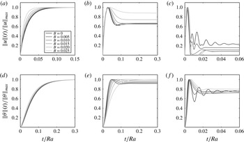
Development of
 $\Vert \boldsymbol{u}\Vert$
and
 $\Vert {\it\theta}\Vert$
after the reduction of yield stress to
 $B=B_{1}<B_{cr}$
at
 $t=0$
: (a,d)
 $\mathit{Ra}=10^{2}$
; (b,e)
 $10^{4}$
; (c,f)
 $10^{6}$
.

4.1. Onset of natural convection from a conductive state
In the first case, at
 $t=0$
yield stress is reduced from
 $B_{0}>B_{cr}$
to a value less than the critical limit,
 $B_{1}<B_{cr}$
. This causes a transition from the purely conductive to a convective state. Transition of
 $\Vert \boldsymbol{u}\Vert (t)$
and
 $\Vert {\it\theta}\Vert (t)$
from the static state to the steady convective state is illustrated in figure 4. Recall that the final steady-state solutions are illustrated in appendix B. Considering the Newtonian case (
 $B=0$
), we see that for small values of Rayleigh number,
 $\Vert \boldsymbol{u}\Vert$
and
 $\Vert {\it\theta}\Vert$
increase monotonically to their steady-state value. For moderate values of Rayleigh number the norms increase sharply to a maximum value before slowly decreasing to the steady state. At large values of Rayleigh number, the solution is oscillatory in time but still converges to a steady state. As the Rayleigh number increases the ratio of the initial maximum to the steady-state value increases, i.e. the relative amplitude of the oscillation about the steady state is magnified.
At any given
 $\mathit{Ra}$
, introduction of a yield stress results in an increase of effective viscosity. When the smart fluid is not activated, there is no yield stress and the nominal
 $\mathit{Ra}$
and effective
 $\mathit{Ra}$
(
 $\mathit{Ra}_{e}$
) are the same. As
 $B$
is increased to the critical value, effective viscosity increases,
 $\mathit{Ra}_{e}$
decreases gradually and as
 $B$
approaches the critical limit we have
 $$\begin{eqnarray}\lim _{B\rightarrow B_{cr}^{-}}\mathit{Ra}_{e}=0.\end{eqnarray}$$
At low to moderate
 $\mathit{Ra}$
, stronger viscous dissipation results in damping of the oscillations observed in
 $\Vert \boldsymbol{u}\Vert$
and slower convergence of
 $\Vert T\Vert$
to the steady state (see e.g. figure 4,
 $\mathit{Ra}=10^{2}$
and
 $\mathit{Ra}=10^{4}$
).
At high
 $\mathit{Ra}$
, the magnitude of the oscillations in
 $\Vert \boldsymbol{u}\Vert$
and
 $\Vert {\it\theta}\Vert$
is decreased due to improved (effective) viscous dissipation. Interestingly, this results in faster convergence to the steady state as smaller oscillations are completely smoothed out. Another interesting observation is the presence of an intermediate static state at sufficiently high
 $B$
and
 $\mathit{Ra}$
(see e.g. figure 4
c). This can be explained considering the total kinetic energy of the flow:
 $$\begin{eqnarray}\frac{\mathit{Ra}}{\mathit{Pr}}\frac{\partial H}{\partial t}=-B\langle \dot{{\it\gamma}}\rangle -\langle \dot{{\it\gamma}}^{2}\rangle +\langle u_{2}T\rangle .\end{eqnarray}$$
On increasing
 $\mathit{Ra}$
, oscillations in velocity norm of the Newtonian regime become increasingly stronger. Since introduction of a yield stress is equivalent to decreasing
 $\mathit{Ra}_{e}$
, it decreases the magnitude of velocity norm at the maximum by increasing the effective viscosity and thus enhancing energy dissipation. It also decreases the magnitude of the norm at the minimum. Notice in (4.2) that the effect of plastic dissipation is more dominant at lower
 $\langle \dot{{\it\gamma}}\rangle$
. Therefore, at sufficiently high
 $B$
, kinetic energy dissipation becomes strong enough to decelerate the flow to the point of complete stoppage. The temperature field then develops conductively until the fluid yields again and flow restarts.
Regardless of the value of
 $\mathit{Ra}$
and
 $B$
, we see that the steady state is achieved by
 $t\approx 0.2Ra$
. In general these timescales will depend on
 $\mathit{Pr}$
, which is set to one here. Effect of
 $\mathit{Pr}$
on timescales is discussed in § 5.
4.2. Complete suppression of natural convection
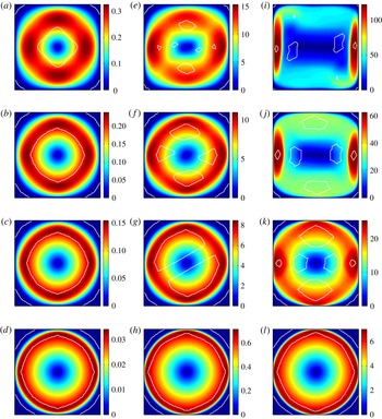
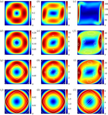
Figure 5 presents some snapshots of the velocity field and plug regions during this transition. In a square cavity the shape, position and size of the plugs all seem to depend on both
 $\mathit{Ra}$
and
 $B$
. The commonality is the presence of a rotating central plug separated by a thin yielded layer from the static unyielded regions at the corners of the cavity shortly before complete stoppage. As the stopping process unfolds the unyielded regions grow progressively larger, the central region forms and eventually the central plug touches the static layer surrounding it and the flow stops. An interesting feature is that the final non-zero velocity fields are representative of the optimal velocity fields defining
 $B_{cr}$
. This is reminiscent of a linear viscous decay where higher frequency modes decay faster leaving a dominant mode at long times.
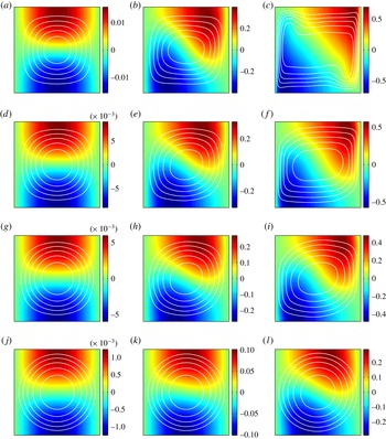
Colourmaps of
 $\mathit{Ra}\Vert \boldsymbol{u}\Vert$
at intermediate stages in the transition from the steady Newtonian flow to a completely static state, due to the introduction of a large yield stress
 $B=0.075$
at
 $t=0$
: (a)
 $Ra=10^{2}$
,
 $t=0.1$
; (b)
 $Ra=10^{2}$
,
 $t=0.25$
; (c)
 $Ra=10^{2}$
,
 $t=0.40$
; (d)
 $Ra=10^{2}$
,
 $t=0.65$
; (e)
 $Ra=10^{4}$
,
 $t=4$
; (f)
 $Ra=10^{4}$
,
 $t=10$
; (g)
 $Ra=10^{4}$
,
 $t=14$
; (h)
 $Ra=10^{4}$
,
 $t=28$
; (i)
 $t=27$
; (j)
 $Ra=10^{6}$
,
 $t=57$
; (k)
 $Ra=10^{6}$
,
 $t=87$
; (l)
 $Ra=10^{6}$
,
 $t=117$
. White curves represent the yield surfaces;
 $\mathit{Pr}=1$
.

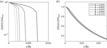
Figure 6 illustrates the development of velocity and temperature norms due to introduction of a yield stress
 $B_{1}>B_{cr}$
at
 $t=0$
. The flow is initially in the steady Newtonian convective state (
 $B_{0}=0$
) and at
 $t=0$
the yield stress
 $B_{1}$
is switched on. In accordance with the analysis presented in § 3.2.1, the kinetic energy decays to zero within a finite time. As predicted by the theoretical results, the decline is more rapid for larger
 $B$
. The decay of
 $\Vert {\it\theta}\Vert (t)$
experiences a brief period where convection is still active, followed by a longer period of pure exponential decay (conductive regime) as the linear temperature profile is approached.
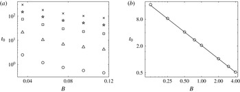
Figure 7(a) illustrates the variation of stopping time with
 $\mathit{Ra}$
and
 $B$
. The stopping time decreases with increasing
 $B$
and decreasing
 $\mathit{Ra}$
. Once the flow has stopped completely, the internal energy decays exponentially and thus contributes the longer timescale of the system.
The plastic dissipation rate of kinetic energy is linearly proportional with
 $B$
. It is therefore expected that the stopping time decreases with increasing Bingham number. In § 3.2.1 we showed that for sufficiently large
 $B$
the stopping time is proportional to
 $B^{-1}$
(note that here
 $\Vert {\it\tau}_{b}\Vert _{\infty }=0$
), as verified in figure 7(b).
The variation of stopping time with
 $\mathit{Ra}$
is best understood with reference to the initial Newtonian state. Before the introduction of the yield stress at
 $t=0$
, the flow is steady and the fluid is Newtonian (
 $B=0$
), so that we have the following balance
 $$\begin{eqnarray}0=-\langle \dot{{\it\gamma}}^{2}\rangle +\langle u_{2}T\rangle ,\end{eqnarray}$$
between viscous dissipation and buoyancy, respectively. For
 $t>0$
the yield stress is increased to
 $B>0$
and the kinetic energy of the flow satisfies (4.2). As the flow is convecting, we may expect that the rate of plastic dissipation (
 $B\langle \dot{{\it\gamma}}\rangle$
) is non-zero. Thus, the balance of (4.3) is broken and the kinetic energy decays.
Development of (a)
 $\Vert \boldsymbol{u}\Vert$
and (b)
 $\Vert {\it\theta}\Vert$
after the introduction of
 $B_{1}>B_{cr}$
at
 $t=0$
at
 $\mathit{Ra}=10^{4}$
. Decay trends are quite similar at lower and higher
 $\mathit{Ra}$
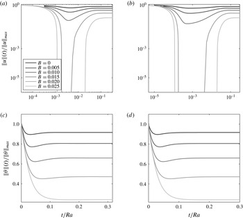
. The main differences being (1) the magnitude of
 $t_{0}$
which determines the extent of effect of advection and (2) the conductive time scale.

(a) Variation of stopping time with Bingham number at
 $\mathit{Ra}=10^{2}$
(○),
 $\mathit{Ra}=10^{3}$
(▵),
 $\mathit{Ra}=10^{4}$
(▫),
 $\mathit{Ra}=10^{5}$
(✩) and
 $\mathit{Ra}=10^{6}$
(
 $\times$
). (b) Stopping time versus
 $B$
at
 $\mathit{Ra}=10^{4}$
. The symbols represent the computed values and the solid line is a fitted curve:
 $t_{0}=2.06/B$
. Here
 $\mathit{Pr}=1$
.

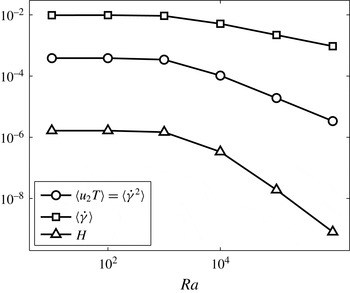
Variation with
 $\mathit{Ra}$
of the kinetic energy and other contributing terms in the energy balance at
 $t=0$
(
 $B=0$
,
 $\mathit{Pr}=1$
).

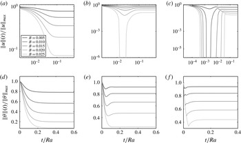
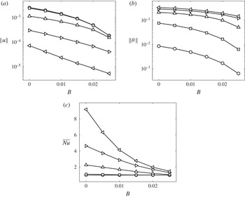
Deceleration of Newtonian convective field by introduction of
 $B<B_{cr}$
to a steady convective viscoplastic field, with
 $\mathit{Pr}=1$
: (a,d)
 $\mathit{Ra}=10^{2}$
; (b,e)
 $\mathit{Ra}=10^{4}$
; (c,f)
 $\mathit{Ra}=10^{6}$
.

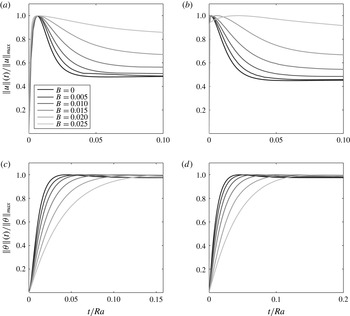
Effect of
 $\mathit{Pr}$
on transition from pure conduction to steady convection in a square cavity at
 $\mathit{Ra}=10^{4}$
: (a,c)
 $\mathit{Pr}=10$
; (b,d)
 $\mathit{Pr}=100$
.

For the initial steady state figure 8 evaluates the functionals
 $\langle u_{2}T\rangle$
,
 $\langle \dot{{\it\gamma}}\rangle$
and
 $H$
. We see that at low to moderate values of
 $\mathit{Ra}$
, both the kinetic energy and plastic dissipation change negligibly with
 $\mathit{Ra}$
. The rate of change of kinetic energy is inversely proportional to
 $\mathit{Gr}=\mathit{Ra}/\mathit{Pr}$
. Since
 $\mathit{Pr}$
is constant here, the stopping time increases almost linearly with
 $\mathit{Ra}$
. At higher values of
 $\mathit{Ra}$
however, the initial kinetic energy decreases faster than the plastic dissipation. Thus, the increase in stopping time with
 $\mathit{Ra}$
is less than linear. It is also interesting to remark that although for larger
 $\mathit{Ra}$
the maximum velocity increases, the kinetic energy decreases with Rayleigh number. This is due to the formation of a boundary layer close to the side walls, outside of which velocity gradients are relatively small.
4.3. Partial suppression of natural convection
Figure 9 shows examples where a yield stress
 $B_{1}<B_{cr}$
is introduced at
 $t=0$
to a steady Newtonian regime. The result is the deceleration of the flow to a new steady state with smaller maximum velocity, weaker convection and thus lower Nusselt number than the initial state. Thus, instead of a simple on–off control of natural convection in principle we should be able to control to any
 $\overline{\mathit{Nu}}$
between the conductive and initial Newtonian state.
Note however that transition between the two steady states is not necessarily monotonic. For smaller values of Rayleigh number (see for example figure 9, with
 $\mathit{Ra}=10^{2}$
), the norms decay monotonically to the steady value. However, for larger values of Rayleigh number, the norms initially decay relatively sharply to a minimum less than the steady value. Relative strength of plastic dissipation of kinetic energy at
 $t=0$
increases with increasing
 $B$
and
 $\mathit{Ra}$
(see (4.2) and figure 8). Thus, the relative value of the minima decreases with increasing Bingham and Rayleigh numbers. For sufficiently large Rayleigh and Bingham numbers, the minimum of the kinetic energy reaches zero: for an intermediate time interval the fluid becomes static everywhere in the domain; see e.g. figure 9(b,c). The norms then increase more slowly to the steady limit.
Once the fluid becomes unyielded everywhere, heat transfer is purely conductive and static state is temporarily sustained. While the temperature field approaches the linear distribution buoyancy stresses are balanced by the plastic stresses, see (2.1). However, the Bingham number is not high enough to balance the buoyancy force in the conductive limit (
 $B<B_{cr}$
). Therefore, as the temperature field approaches the conductive limit, it yields the fluid and the flow restarts, resulting in the increase of kinetic energy from zero up to the new steady-state value.
5. Effect of Prandtl number
Having established the main principles of this method at
 $\mathit{Pr}=1$
, we now consider the effects of varying Prandtl number on the transition between Newtonian and viscoplastic steady states.
It was discussed in § 2.3 that advection of momentum is negligible in comparison with diffusion of momentum for the range of
 $\mathit{Pr}$
considered here (
 $1\leqslant \mathit{Pr}\leqslant 100$
). The changes in steady regime with
 $\mathit{Pr}$
are therefore not noticeable. Since the Prandtl number represents the relative strength of viscous to thermal diffusion rates, we expect this parameter to principally affect the relative behaviour of
 $\Vert \boldsymbol{u}\Vert$
and
 $\Vert {\it\theta}\Vert$
in transition.
The development of the steady Newtonian convection from a static state is illustrated in figures 10 and 11 at different values of
 $\mathit{Pr}$
, i.e. deactivating. The effect of
 $\mathit{Pr}$
is more pronounced on
 $\Vert \boldsymbol{u}\Vert$
than on
 $\Vert {\it\theta}\Vert$
. We can think of
 $\mathit{Pr}$
as the ratio of the response timescale of temperature and velocity fields, both to external forcing; i.e. the larger the Prandtl number, the faster velocity field adapts to the buoyancy forces caused by an imposed temperature field, and vice versa. However, as the velocity and temperature are fully coupled via buoyancy, variation of the transition timescales with
 $\mathit{Pr}$
deviates from the linear trend otherwise expected. Nonetheless, we see the faster initial response of velocity with increasing
 $\mathit{Pr}$
; i.e. the increasingly sharp initial jump in
 $\Vert \boldsymbol{u}\Vert$
. The quick development of the velocity field advances heat transfer by advection.
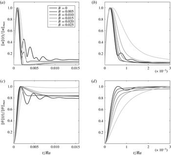
Also, note in figure 10 that the oscillations in velocity and temperature norm at high
 $\mathit{Ra}$
decline at higher
 $\mathit{Pr}$
. Lower values of
 $\mathit{Pr}$
allow the coupling of the partial time derivatives of momentum and heat equations. When the
 $\mathit{Pr}$
is too large, the left-hand side of momentum equation diminishes too quickly and development of the flow is dominated by the transition of temperature field. With weaker oscillation, the intermediate static state (previously observed in figure 4) disappears.
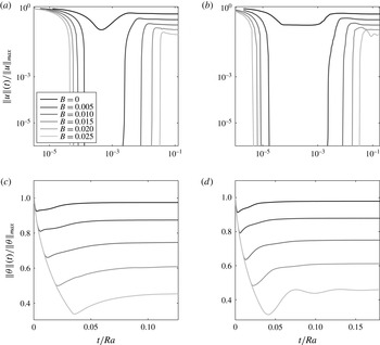
Effect of
 $\mathit{Pr}$
on transition from pure conduction to steady convection in a square cavity at
 $\mathit{Ra}=10^{6}$
: (a,c)
 $\mathit{Pr}=10$
; (b,d)
 $\mathit{Pr}=100$
.

Figures 12 and 13 explore the effect of introducing a subcritical yield stress (
 $B<B_{cr}$
) to the Newtonian steady convective flow
 $t=0$
. The effects are quite marked. At sufficiently low
 $\mathit{Pr}$
the velocity approaches the new steady state smoothly with no over-shoot. Increasing
 $B$
, we see an increasingly rapid initial evolution. This results in the temporary arrest of the flow (as discussed earlier), followed by a conductive restart. At larger
 $\mathit{Pr}$
the flow stops more quickly, but the restart time is controlled by conduction and hence is unaffected; e.g. compare figure 12(b,c). Note that we have already seen that at low to moderate
 $\mathit{Ra}$
the steady states are not affected greatly by
 $\mathit{Pr}$
and thus the initial (Newtonian) energy balance for these simulations is similar. On introducing the positive yield stress into the transient problem at a given
 $\mathit{Ra}$
, the only difference that depends on
 $\mathit{Pr}$
is in the response time of the kinetic energy (or
 $\Vert \boldsymbol{u}\Vert$
), scaling with
 $1/\mathit{Pr}$
. This explains the decrease in timescale of the initial transient with increasing
 $\mathit{Pr}$
.
Effects of introduction of subcritical yield stress (
 $B<B_{cr}$
) on the steady convective Newtonian flow at
 $\mathit{Ra}=10^{4}$
: (a,c)
 $\mathit{Pr}=10$
; (b,d)
 $\mathit{Pr}=100$
. For
 $\mathit{Pr}=1$
see figure 9(b,e).

Effects of introduction of a subcritical yield stress (
 $B<B_{cr}$
) on the steady convective Newtonian flow at
 $\mathit{Ra}=10^{6}$
: (a,c)
 $\mathit{Pr}=10$
; (b,d)
 $\mathit{Pr}=100$
. For
 $\mathit{Pr}=1$
see figure 9(c,f).

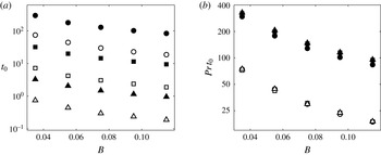
Introduction of a large yield stress
 $B>B_{cr}$
results in stopping of the flow field within a finite time. Transition trends are qualitatively similar to those presented previously in figure 5. The computed stopping times
 $t_{0}$
, at different
 $\mathit{Pr}$
, are presented in figure 14. As discussed earlier, from the energy equation (3.25), we have that the rate of change of kinetic energy is proportional to
 $\mathit{Pr}$
, i.e. increasing viscosity improves the diffusion of momentum. Also, for the initial condition and Bingham numbers considered here rate of change of kinetic energy is considerably faster than that of internal energy. Therefore, the temperature field that causes kinetic energy production, through the buoyancy term in (4.2), can be treated as a constant during the stopping process. Stopping time is thus inversely proportional to
 $\mathit{Pr}$
(see figure 14
b).
Variation of computed stopping time
 $t_{0}$
with Bingham number
 $B>B_{cr}$
for
 $\mathit{Pr}=1$
(○),
 $\mathit{Pr}=10$
(▵) and
 $\mathit{Pr}=100$
(▫). Empty and filled markers represent
 $\mathit{Ra}=10^{4}$
and
 $\mathit{Ra}=10^{6}$
, respectively.

6. Summary
In this paper we have introduced the idea of a novel regulation of heat transfer across a cavity, by using a controllable yield stress in order to suppress the advective component of heat transfer. Using this method we may expect to vary the averaged Nusselt number by a factor of 7–10, in moving from fully conductive to convective regimes. We have used both analytical and computational methodologies to study the feasibility of the flow control.
On the theoretical side, we have demonstrated that above a given critical limit,
 $B=B_{cr}$
, the steady solution to the coupled Navier–Stokes and energy equations is static and purely conductive. It is only for
 $B<B_{cr}$
that steady advective motion can be found. The critical value
 $B_{cr}$
depends upon the domain geometry, but is independent of the other dimensionless problem parameters (
 $\mathit{Ra}$
and
 $\mathit{Pr}$
). The parameter
 $B$
represents the balance of yield stress to buoyancy stress, so it is intuitive that this balance controls the occurrence of static states. Our results give a clear definition of this limit, establishing the theoretical basis on which advection can be suppressed.
As an aside, Huilgol & Kefayati (Reference Huilgol and Kefayati2015) also consider the critical Bingham number (denoted
 $\mathit{Bn}$
) in a square cavity and examine its variation with
 $\mathit{Ra}$
and
 $\mathit{Pr}$
. Their parameter
 $\mathit{Bn}$
is given by
 $$\begin{eqnarray}\mathit{Bn}=\frac{\sqrt{2}\hat{{\it\tau}}_{y}\hat{L}}{\hat{{\it\mu}}\sqrt{{\hat{g}}\hat{L}\hat{{\it\beta}}{\rm\Delta}\hat{T}}}=B\sqrt{2\frac{\mathit{Ra }}{\mathit{Pr}}}.\end{eqnarray}$$
They observe a variation of
 $\mathit{Bn}$
with both
 $\mathit{Ra}$
and
 $\mathit{Pr}$
, suggesting an empirical relationship between the three dimensionless parameters (
 $\mathit{Bn}=0.152\mathit{Ra}^{0.37}\mathit{Pr}^{-0.39}$
). This expression does not capture the physical correlations correctly; i.e. since
 $B_{cr}$
is independent of
 $\mathit{Ra}$
and
 $\mathit{Pr}$
,
 $\mathit{Bn}_{cr}\sim \mathit{Ra}^{0.5}\mathit{Pr}^{-0.5}$
. The deviation of their numerical results from the exact value of
 $\mathit{Bn}$
is most noticeable at
 $\mathit{Ra}=10^{3}$
, where they overestimate
 $\mathit{Bn}$
by more than 100 %.
Second, we have examined the stability of the conductive steady states found for
 $B>B_{cr}$
, showing that the transients should decay to zero, either for sufficiently small initial conditions, or for sufficiently small Rayleigh number
 $\mathit{Ra}$
. We also demonstrate that when the static conductive steady state is stable, the kinetic energy decays to zero in a finite time. We provide an analytical expression estimating the stopping time
 $t_{0}$
.
The tools that we use to study the flow stability are drawn from functional analysis and the various constants (such as
 $C_{P}$
,
 $\tilde{C}_{P}$
and
 $C_{TS}$
) are order one, positive and depend only on the domain shape and dimension. Although we have concentrated on rectangular cavities for simplicity, this analytical framework can easily be extended to cavities of other shapes and we may expect a similar qualitative behaviour. In generalizing, the various bounds, the critical
 $B$
and decay rates will naturally depend on the domain shape and also on the gradient of the steady conductive state.
We have also used computational simulations to resolve the Navier–Stokes and energy equations for different yield stresses
 $B$
, and for imposed changes in
 $B$
. This has helped illustrate the processes of stopping and starting the flow, as well as providing more concrete estimates of the timescales and examples of flow transitions. Furthermore, computations have been used to evaluate
 $B_{cr}$
for different aspect ratio cavities (appendix B). Further computations have explored the effects of varying
 $\mathit{Pr}$
.
In terms of controlling the transients, we have simply implemented step changes in
 $B$
and allowed the system to respond. We may consider the system of coupled energy equations (kinetic and internal) to be effectively a first-order system. Hence, on imposing step changes, we should not be surprised to find noticeable transient overshoots in
 $\Vert \boldsymbol{u}\Vert (t)$
,
 $\Vert {\it\theta}\Vert (t)$
and
 $\overline{\mathit{Nu}}(t)$
in attaining each new steady state. These overshoots increase with
 $\mathit{Ra}$
and are a consequence of the simple open-loop control. We expect that a more sophisticated control would be able to significantly reduce this feature. In total, the theoretical and computational results establish that this methodology is hydrodynamically feasible for the control of heat transfer.
In presenting the idea we have assumed a rheology for which the yield stress can be varied rapidly. It has been our intention to not focus on any specific fluid type, but instead on the dynamics. Having said this, the type of effect required may be achieved with electro-rheological or magneto-rheological (ER/MR) fluids, which have very rapid response times. Of course, we acknowledge that the rheological descriptions we have used are quite simplistic in dealing with smart viscoplastic fluids of this nature. Nevertheless, we now examine some typical physical parameters.
The carrier fluid in ER/MR fluids is most commonly a silicone oil (de Vicente, Klingenberg & Hidalgo-Alvarez Reference de Vicente, Klingenberg and Hidalgo-Alvarez2011; Sheng & Wen Reference Sheng and Wen2012). Fluid properties vary by smart fluid design, but typical values are
 $$\begin{eqnarray}\left.\begin{array}{@{}c@{}}{\it\mu}\approx 10^{-2}~\text{Pa}~\text{s},\quad {\it\rho}\approx 10^{3}~\text{kg}~\text{m}^{-3},\quad c_{P}\approx 1.5\times 10^{3}~\text{J}~\text{kg}^{-1}~\text{K}^{-1},\\ k\approx 0.15~\text{W}~\text{m}^{-1}~\text{K}^{-1},\quad {\it\beta}\approx 10^{-3}~\text{K}^{-1}.\end{array}\right\}\end{eqnarray}$$
If we take a square cavity of side
 $\hat{L}=1.5$
cm and impose a temperature difference
 ${\rm\Delta}\hat{T}=35$
K the Rayleigh number would be
 $\mathit{Ra}\approx 10^{6}$
. The velocity responds rapidly, on a timescale
 $\propto \mathit{Ra}/\mathit{Pr}$
, but this still waits for the thermal response that occurs on a timescale of the order of
 $0.2\mathit{Ra}$
. In this case this is less than
 $400$
s. The shortest hydrodynamic timescale is that of stopping. At
 $B=0.055$
the dimensionless stopping time is approximately two time units. This is equivalent to about 4 ms, which is fast and close to the typical rheological response times of smart fluid. The yield stress required to change the Bingham number by
 ${\rm\Delta}B=0.1$
in this configuration is about 0.5 Pa. To vary the Bingham number from zero to a value
 $B=1$
, it suffices to activate the fluid to achieve a yield stress of 5 Pa. Typical timescales for pure conduction are
 ${\sim}10^{3}~\text{s}$
for geometries such as that discussed above, so we see that advection is needed to accelerate startup. Equally, in waiting to see whether flows have really stopped, relatively long conductive times are needed.
Note that the yield stresses are relatively modest in examples such as that above. The key balance is buoyancy to yield stress, and the buoyancy force is relatively limited. This puts this particular application of smart yield stress fluids in a different category than many other applications, where high performance requires that large yield stresses are developed very quickly (ER/MR clutches, valves, active damping, etc.). Here it is likely to be more important to be able to control the yield stress effectively over a range of
 ${\sim}100~\text{Pa}$
. Larger yield stresses do of course shorten the stopping time, but in any case if the stopping time becomes comparable with the rheological activation timescale of the fluid, then the assumption made of instantaneous switching of
 $B$
becomes questionable. The main restriction in application of this methodology is probably the relatively long thermal response time for the onset of advection: switching off the advective field is much more rapid than retrieving the steady convective regime. Essentially, it is easier to control the momentum transfer than the heat transfer.
Acknowledgements
We gratefully acknowledge financial support of the Natural Sciences and Engineering Research Council of Canada. I. K. acknowledges the support of the University of British Columbia via a 4YF graduate fellowship. I. F. acknowledges the financial support of LABEX iMUST (ANR-10-LABX-0064) of Université de Lyon, within the program ‘Investissements d’Avenir’ (ANR-11-IDEX-0007) operated by the French National Research Agency (ANR). This research was enabled in part by support provided by WestGrid (http://www.westgrid.ca) and Compute Canada/Calcul Canada (http://www.computecanada.ca). We thank the reviewers for their helpful comments.
Appendix A. Computational method
The set of aforementioned governing equations and corresponding boundary conditions is solved using an augmented Lagrangian algorithm combined with a finite volume/staggered grid space discretization. We have used a uniform mesh of size
 $100\times 100$
for all simulations. The numerical strategy employed here is very similar to that in Vinay et al. (Reference Vinay, Wachs and Agassant2005), except that in this work the momentum and energy equations are two-way coupled by the buoyancy term and the problem is posed in a planar geometry instead of an axisymmetric one.
The principle of the augmented Lagrangian algorithm is to recast the whole fluid flow problem into a minimization problem of a functional. In practice, we introduce an additional strain-rate tensorial field
 $d$
representing the true deformation undergone by the material. The solution of the problem is calculated as a saddle-point
 $(u,p,d,{\it\lambda})$
of the minimization problem with a Uzawa-like algorithm. Here
 ${\it\lambda}$
is an additional Lagrange multiplier tensorial field that enforces
 $d$
to equal
 $D(u)$
, i.e. it relaxes the constraint
 $d-D(u)=0$
as
 $p$
relaxes the constraint
 $(\partial u_{i}^{n+1,k+1}/\partial x_{i})=0$
. It can be interpreted at the physical level as a plastic stress. The original functional is augmented by adding an additional quadratic term
 $0.5r|d-D(u)|^{2}$
to speed up the convergence rate of the Uzawa algorithm, where
 $r$
stands for the augmentation parameter (once again, for a detailed presentation of the construction of augmented Lagrangian algorithm, see Vinay et al. (Reference Vinay, Wachs and Agassant2005) or Glowinski & Wachs (Reference Glowinski and Wachs2011) and the references therein). Assuming that
 ${\it\Omega}$
denotes the flow domain and omitting the boundary conditions for the sake of conciseness, the complete solution algorithm hence reads as follows.
-
(1) Time loop
$t^{n+1}=t^{n}+{\rm\Delta}t$
,
$n\geqslant 0$
.-
(i) Initialization of:
$u^{n+1,0}=u^{n}$
and
${\it\lambda}^{n+1,0}={\it\lambda}^{n}$
. -
(ii) Solve the viscoplastic Navier–Stokes problem with the following augmented Lagrangian algorithm:
$k\geqslant 0$
.-
(1) Solve the following Navier–Stokes problem: find
$u^{n+1,k+1}$
and
$p^{n+1,k+1}$
such that (A 1)
$$\begin{eqnarray}\displaystyle & \displaystyle Gr\frac{u^{n+1,k+1}-u^{n}}{{\rm\Delta}t}+\frac{\partial p^{n+1,k+1}}{\partial x_{i}}-(2+r)D(u^{n+1,k+1}) & \displaystyle \nonumber\\ \displaystyle & \displaystyle \quad =-Gr\;u_{j}^{n}\frac{\partial u_{i}^{n}}{\partial x_{j}}+B({\it\lambda}^{n+1,k}-rd^{n+1,k})+T^{n}{\it\delta}_{i2} & \displaystyle\end{eqnarray}$$
(A 2)
$$\begin{eqnarray}\displaystyle & \displaystyle \frac{\partial u_{i}^{n+1,k+1}}{\partial x_{i}}=0. & \displaystyle\end{eqnarray}$$
-
(2) Update
$d^{n+1,k+1}$
by (A 3)
$$\begin{eqnarray}\hspace{-12.0pt}d^{k+1,n+1}=\left\{\begin{array}{@{}l@{}}0\quad \text{if }|{\it\lambda}^{n+1,k}+rD(u^{n+1,k+1})|<B\quad \\ \displaystyle \frac{1}{r}\left(\!1-\frac{B}{|{\it\lambda}^{n+1,k}+rD(u^{k+1,n+1})|}\right)\!({\it\lambda}^{n+1,k}+rD(u^{n+1,k+1}))\quad \text{if not }\quad \end{array}\right.\end{eqnarray}$$
-
(3) Update the Lagrange multiplier
${\it\lambda}^{n+1,k+1}$
(A 4)
$$\begin{eqnarray}{\it\lambda}^{n+1,k+1}={\it\lambda}^{n+1,k}+r(D(u^{n+1,k+1})-d^{n+1,k+1}).\end{eqnarray}$$
-
(4) Convergence if
(A 5)
$$\begin{eqnarray}\displaystyle & \displaystyle D(u,p)^{k+1}=\max _{{\it\Omega}}|u^{n+1,k+1}-u^{n+1,k}|+\max _{{\it\Omega}}|p^{n+1,k+1}-p^{n+1,k}|\leqslant {\it\epsilon}_{1} & \displaystyle \nonumber\\ \displaystyle & & \displaystyle\end{eqnarray}$$
(A 6)
$$\begin{eqnarray}\displaystyle & \displaystyle {\rm\Delta}D^{k+1}=\max _{{\it\Omega}}|D(u^{n+1,k+1})-d^{n+1,k+1}|\leqslant {\it\epsilon}_{2}. & \displaystyle\end{eqnarray}$$
-
-
(iii) Set:
$u^{n+1}=u^{n+1,k+1}$
,
$p^{n+1}=p^{n+1,k+1}$
and
${\it\lambda}^{n+1}={\it\lambda}^{n+1,k+1}$
-
(iv) Solve the energy equation: find
$T^{n+1}$
such that (A 7)
$$\begin{eqnarray}\mathit{Ra}\frac{T^{n+1}-T^{n}}{{\rm\Delta}t}-\frac{\partial T^{n+1}}{\partial x_{i}\partial x_{i}}=-\mathit{Ra}\;u_{i}^{n+1}\frac{\partial T^{n}}{\partial x_{i}}.\end{eqnarray}$$
-
-
(2) END.


Appendix B. Features of the steady convective state
It was established in § 2.3 that features of the steady-state regimes vary negligibly with
 $\mathit{Pr}$
. For this reason, results are presented at
 $\mathit{Pr}=1$
here. Steady regimes at higher values of
 $\mathit{Pr}$
are expected to be quite similar to those presented here.
For
 $B=0$
and
 $\mathit{Ra}\in [10^{2},10^{6}]$
we initialize our computations from the conductive temperature and static fluid and integrate forward, until a steady state is achieved. For
 $B>0$
we use the corresponding steady Newtonian convective solution as initial condition, again evolving forward until a steady state is achieved. Figures 15 and 16 illustrate the steady-state speed and temperature (
 ${\it\theta}=T+x$
) fields in a square cavity, computed at different values of
 $\mathit{Ra}$
and
 $B$
for
 $\mathit{Pr}=1$
.
Colourmaps of
 $\mathit{Ra}\Vert u\Vert$
and the yield surface (white solid lines) at different
 $\mathit{Ra}$
and
 $B$
: (a,d,g,j)
 $\mathit{Ra}=10^{2}$
; (b,e,h,k)
 $\mathit{Ra}=10^{4}$
; (c,f,i,l)
 $\mathit{Ra}=10^{6}$
; (a–c)
 $B=0$
; (d–f)
 $B=0.010$
; (g–i)
 $B=0.015$
; (j–l)
 $B=0.025$
.

Colourmaps of
 ${\it\theta}$
and superimposed streamlines (white solid lines) at different
 $\mathit{Ra}$
and
 $B$
: (a,d,g,j)
 $\mathit{Ra}=10^{2}$
; (b,e,h,k)
 $\mathit{Ra}=10^{4}$
; (c,f,i,l)
 $\mathit{Ra}=10^{6}$
; (a–c)
 $B=0$
; (d–f)
 $B=0.010$
; (g–i)
 $B=0.015$
; (j–l)
 $B=0.025$
.

At
 $B=0$
(Newtonian) as
 $\mathit{Ra}$
is increased the flows become progressively asymmetrical with sharp boundary layers at the walls. Increasing
 $\mathit{Ra}$
represents the dominance of advective effects over conductive effects in the boundary layers that form. Variation of the
 $L^{2}$
norm of
 $\boldsymbol{u}$
and
 ${\it\theta}$
and the average Nusselt number are summarized in figure 17, for varying
 $B$
. The magnitude of both
 $\boldsymbol{u}$
and
 ${\it\theta}$
is reduced as
 $B$
is increased. This is not surprising as increasing
 $B$
results in an increase of the effective viscosity.
Also note that in figure 17(a) the magnitude of
 $\boldsymbol{u}$
decreases with increasing
 $\mathit{Ra}_{e}$
. As the yield stress is increased from zero toward the critical limit, the effective Rayleigh number
 $\mathit{Ra}_{e}$
varies from the Newtonian value (
 $\mathit{Ra}$
) to zero at
 $B\geqslant B_{cr}$
.
For
 $B\lessapprox B_{cr}$
, we may assume
 $\mathit{Ra}_{e}$
to be relatively small, there are no boundary layers and it is reasonable to assume:
 $$\begin{eqnarray}l_{1}\approx l_{2}=1.\end{eqnarray}$$
As
 $B$
decreases, the effective
 $\mathit{Ra}_{e}$
attains moderate values. In this range we see that
 $\Vert {\it\theta}\Vert$
increases almost linearly with
 $\mathit{Ra}$
(figure 17
b) while
 $\Vert \boldsymbol{u}\Vert$
remains constant; see (2.14) and figure 17(a). Finally, as
 $\mathit{Ra}_{e}$
increases towards
 $\mathit{Ra}$
for insignificant
 $B$
,
 $\Vert {\it\theta}\Vert$
approaches a maximum value as boundary layers form on the vertical walls. Hence, we find
 $$\begin{eqnarray}l_{1}\ll l_{2}=1.\end{eqnarray}$$
It can be inferred from the works of Gill (Reference Gill1966) and Karimfazli & Frigaard (Reference Karimfazli and Frigaard2013) that at high
 $\mathit{Ra}_{e}$
, it is conservative to assume
 $$\begin{eqnarray}l_{1}\propto \mathit{Ra}_{e}^{-1/4}\propto \mathit{Ra}^{-1/4}.\end{eqnarray}$$
Therefore,
 $U_{2}$
decreases with increasing
 $\mathit{Ra}$
at a rate slower than
 $\mathit{Ra}^{-1}$
. This may seem to be in contradiction with the results of Turan et al. (Reference Turan, Chakraborty and Poole2010), where velocity increases with
 $\mathit{Ra}$
. However, this apparent discrepancy is due to different definitions of the dimensionless variables: the results are in fact consistent.
Variation of
 $\Vert \boldsymbol{u}\Vert$
,
 $\Vert {\it\theta}\Vert$
and
 $\mathit{Nu}$
with
 $B$
at
 $\mathit{Ra}=10^{2}$
(○),
 $\mathit{Ra}=10^{3}$
(▫),
 $\mathit{Ra}=10^{4}$
(▵),
 $\mathit{Ra}=10^{5}$
(▹) and
 $\mathit{Ra}=10^{6}$
(◃).

Appendix C. Effect of the aspect ratio
Here we briefly consider the variation of critical Bingham number with aspect ratio and comment on how transient characteristics change. Turan et al. (Reference Turan, Poole and Chakraborty2011) have studied the variation of steady state characteristics of the flow with aspect ratio. Vikhansky (Reference Vikhansky2010a
) has investigated the variation of critical Bingham number with
 $AR$
numerically using a regularized model. Regularized models can only give estimates of plug boundaries and are less reliable as yield stress approaches the critical limit. Table 3 compares our results, calculated using augmented Lagrangian method as described in § 2.2, against the computed estimates of Vikhansky (Reference Vikhansky2010a
). The relative difference of the values is
 ${<}5\,\%$
at all
 $AR$
.
Figure 19 illustrates the velocity field and plug boundaries at Bingham numbers just smaller than
 $B_{cr}$
. Figure 19(a,b) show (near-)semicircular regions at each end, where the fluid is close to rigid motion, separated by a central region where the flow is approximately uniaxial. As
 $AR\rightarrow \infty$
the two end regions remain of
 $O(1)$
as the central region grows and approaches the limiting one-dimensional flow. At this limit, two plugs with opposite velocities separate the yielded layers on the vertical walls and around the symmetry line and
 $B_{cr}=1/16$
. Further, from the development of flow geometry with
 $AR$
we can deduce that the convergence of
 $1/16-B_{cr}$
to zero as
 $AR\rightarrow \infty$
is no faster than
 $AR^{-1}$
.
Variation of
 $B_{cr}$
with aspect ratio of the cavity.

Colourmaps of
 $\mathit{Ra}\Vert \boldsymbol{u}\Vert$
in cavities of different aspect ratio as
 $B\rightarrow B_{cr}^{-}$
,
 $\mathit{Ra}=10^{5}$
,
 $\mathit{Pr}=1$
. The white curves represent yield surfaces: (a)
 $AR=2$
,
 $B=0.0427$
; (b)
 $AR=4$
,
 $B=0.052$
.

Considering transitions, introduction of a non-zero yield stress will have the same qualitative results: transition to a new steady state with lower kinetic energy and
 $\overline{Nu}$
. Depending on
 $\mathit{Ra}$
and
 $B$
this transition may or may not be monotonic. If the introduced yield stress is larger than the critical value, the new steady state will be conductive (
 $\overline{Nu}=1$
).
Critical Bingham number at different aspect ratios. Exact values at
 $AR=1$
and
 $AR\rightarrow \infty$
are
 $0.03125$
and
 $0.0625$
, respectively.

For fixed
 $\mathit{Ra}$
and
 $\mathit{Pr}$
, the kinetic energy is expected to increase with the cavity aspect ratio
 $AR$
. It is therefore expected that the stopping time,
 $t_{0}$
, will increase with the aspect ratio and this is confirmed in figure 20 where the computed
 $t_{0}$
are shown. Figure 21 presents snapshots of the speed contours and yield surfaces as time evolves, when
 $B>B_{cr}$
is introduced. The size of the unyielded regions both in the corners and in the counter-current central region increases in time. The plug regions in the corners grow and merge together, stopping flow completely in the ends. The flow stops everywhere when the moving and static plugs touch. Note that the dissipation rate is zero in the unyielded end plug regions.
Variation of the stopping time
 $t_{0}$
with
 $B$
at different
 $AR$
. Other parameters:
 $\mathit{Ra}=10^{4}$
,
 $\mathit{Pr}=1$
.

Colourmaps of
 $\mathit{Ra}\Vert u\Vert$
at intermediate stages in transition from the steady Newtonian field to a completely static state due to introduction of
 $B=0.075$
at
 $t=0$
: (a)
 $t=8$
; (b)
 $t=18$
; (c)
 $t=28$
; (d)
 $t=38$
; (e)
 $t=18$
; (f)
 $t=38$
; (g)
 $t=58$
; (h)
 $t=78$
. White curves represent the yield surfaces. Other parameters:
 $\mathit{Ra}=10^{4}$
,
 $\mathit{Pr}=1$
,

Appendix D. Proofs
D.1. Proof of theorem 1
Let
 $E=H+Pr\,K$
be the total energy of the system. Combining (3.25) and (3.26) yields
 $$\begin{eqnarray}\frac{\mathit{Ra}}{\mathit{Pr}}\frac{\text{d}E}{\text{d}t}=-\langle \dot{{\it\gamma}}^{2}\rangle -B\langle \dot{{\it\gamma}}\rangle +\langle {\it\tau}_{b,ij}\dot{{\it\gamma}}_{ij}\rangle +\langle u_{2}{\it\theta}\rangle +\mathit{Ra}\langle {\it\theta}u_{1}\rangle -\langle |\boldsymbol{{\rm\nabla}}{\it\theta}|^{2}\rangle .\end{eqnarray}$$
Based on the Poincaré and Korn inequalities, there exist positive constants
 $C_{p}$
and
 $\tilde{C}_{p}$
such that
 $$\begin{eqnarray}\displaystyle & C_{p}\langle \boldsymbol{u}^{2}\rangle \leqslant \langle |\boldsymbol{{\rm\nabla}}\boldsymbol{u}|^{2}\rangle =\langle \dot{{\it\gamma}}^{2}\rangle & \displaystyle\end{eqnarray}$$
 $$\begin{eqnarray}\displaystyle & \tilde{C}_{p}\langle {\it\theta}^{2}\rangle \leqslant \langle |\boldsymbol{{\rm\nabla}}{\it\theta}|^{2}\rangle . & \displaystyle\end{eqnarray}$$
 $\boldsymbol{u}\neq 0$
, there exists a constant
 $C_{TS}$
such that
 $$\begin{eqnarray}C_{TS}\Vert \boldsymbol{u}\Vert \leqslant \langle \dot{{\it\gamma}}\rangle\end{eqnarray}$$
see Temam & Strang (Reference Temam and Strang1980). Using the Cauchy–Schwarz inequality:
 $$\begin{eqnarray}\left.\begin{array}{@{}c@{}}\langle u_{2}{\it\theta}\rangle \leqslant \Vert u_{2}\Vert \,\Vert {\it\theta}\Vert \leqslant \Vert \boldsymbol{u}\Vert \,\Vert {\it\theta}\Vert \\ \langle {\it\theta}u_{1}\rangle \leqslant \Vert {\it\theta}\Vert \,\Vert \boldsymbol{u}\Vert \end{array}\right\}\end{eqnarray}$$
and the Hölder inequality gives
 $$\begin{eqnarray}\langle {\it\tau}_{b,ij}\dot{{\it\gamma}}_{ij}\rangle \leqslant \Vert {\it\tau}_{b}\Vert _{\infty }\langle \dot{{\it\gamma}}\rangle .\end{eqnarray}$$
Combining the above inequalities and equation (D 1) yields
 $$\begin{eqnarray}\frac{\mathit{Ra}}{\mathit{Pr}}\frac{\text{d}E}{\text{d}t}\leqslant (\mathit{Ra}+1)\Vert {\it\theta}\Vert \;\Vert \boldsymbol{u}\Vert -(B-\Vert {\it\tau}_{b}\Vert _{\infty })\;C_{TS}\Vert \boldsymbol{u}\Vert -2\min \left(C_{P},\frac{\tilde{C}_{P}}{Pr}\right)E,\end{eqnarray}$$
for
 $t\geqslant 0$
. Therefore
 $$\begin{eqnarray}\frac{\mathit{Ra}}{\mathit{Pr}}\frac{\text{d}E}{\text{d}t}(0)\leqslant -{\it\alpha}E(0)\quad \text{if}~\Vert {\it\theta}\Vert (0)<\frac{(B-\Vert {\it\tau}_{b}\Vert _{\infty })C_{TS}}{\mathit{Ra}+1},\end{eqnarray}$$
where
 ${\it\alpha}=2\min (C_{P},\tilde{C}_{P}/\mathit{Pr})$
.
This implies that there exists
 ${\it\delta}>0$
such that
 $$\begin{eqnarray}E(t)<E(0)\quad \text{for}~0<t<{\it\delta}.\end{eqnarray}$$
Since
 $E=H+\mathit{Pr}\,K$
, we can infer
 $$\begin{eqnarray}\Vert {\it\theta}\Vert (t)\leqslant \sqrt{\frac{2}{\mathit{Pr}}E(t)}<\sqrt{\frac{2}{\mathit{Pr}}E(0)}.\end{eqnarray}$$
Thus, the assumption
 $$\begin{eqnarray}E(0)<\frac{\mathit{Pr}}{2}\left(\frac{(B-\Vert {\it\tau}_{b}\Vert _{\infty })C_{TS}}{\mathit{Ra}+1}\right)^{2}\end{eqnarray}$$
is sufficient to have
 $$\begin{eqnarray}\frac{\text{d}E}{\text{d}t}(t)<-{\it\alpha}E(t)\quad \text{for }0<t<{\it\delta}.\end{eqnarray}$$
We can now repeat the above argument, starting from
 $t={\it\delta}/2$
. Since all of the former conditions are met, we can enlarge the time interval in which the exponential decay of
 $E(t)$
holds by
 ${\it\delta}$
, thus expanding the internal to
 $t=3{\it\delta}/2$
. We can repeat this indefinitely to show that
 $$\begin{eqnarray}E(t)\leqslant E(0)\exp (-{\it\alpha}t)\quad \text{for}~t\geqslant 0.\end{eqnarray}$$
Combining the above inequality with (D 10) yields
 $$\begin{eqnarray}\Vert {\it\theta}\Vert (t)\leqslant \frac{(B-\Vert {\it\tau}_{b}\Vert _{\infty })C_{TS}}{\mathit{Ra}+1}\exp \left(-\frac{{\it\alpha}}{2}\;t\right)\quad \text{for}~t\geqslant 0.\end{eqnarray}$$
Using inequalities (D 2)–(D 6) and the above inequality together with (3.26) gives
 $$\begin{eqnarray}\frac{\text{d}\Vert \boldsymbol{u}\Vert }{\text{d}t}\leqslant -\frac{C_{p}\,\mathit{Pr}}{\mathit{Ra}}\Vert \boldsymbol{u}\Vert -\frac{(B-\Vert {\it\tau}_{b}\Vert _{\infty })C_{TS}\mathit{Pr}}{\mathit{Ra}+1}.\end{eqnarray}$$
If we denote
 $$\begin{eqnarray}{\it\beta}=\frac{(B-\Vert {\it\tau}_{b}\Vert _{\infty })C_{TS}\mathit{Pr}}{\mathit{Ra}+1}\quad \text{and}\quad {\it\alpha}_{u}=\frac{C_{p}\,\mathit{Pr}}{\mathit{Ra}},\end{eqnarray}$$
then (D 15) implies, via Gronwall’s lemma, that
 $$\begin{eqnarray}\Vert \boldsymbol{u}\Vert (t)\leqslant \left(\Vert \boldsymbol{u}\Vert (0)+\frac{{\it\beta}}{{\it\alpha}_{u}}\right)\exp (-{\it\alpha}_{u}t)-\frac{{\it\beta}}{{\it\alpha}_{u}}.\end{eqnarray}$$
Thus setting
 $$\begin{eqnarray}t_{0}=\frac{1}{{\it\alpha}_{u}}\ln \left(1+\frac{{\it\alpha}_{u}}{{\it\beta}}\Vert \boldsymbol{u}\Vert (0)\right)\end{eqnarray}$$
yields
 $\Vert \boldsymbol{u}\Vert (t)=0$
for
 $t\geqslant t_{0}$
, thus proving the finite time decay of velocity.
D.2. Proof of theorem 2
Using inequalities (D 3)–(D 5) the energy equations (3.25) and (3.26) give the following inequalities:
 $$\begin{eqnarray}\displaystyle & \displaystyle \mathit{Ra}\frac{\text{d}K}{\text{d}t}\leqslant 2\mathit{Ra}\sqrt{KH}-2\tilde{C}_{P}K & \displaystyle\end{eqnarray}$$
 $$\begin{eqnarray}\displaystyle & \displaystyle \frac{\mathit{Ra}}{\mathit{Pr}}\frac{\text{d}H}{\text{d}t}\leqslant -2C_{p}H-C_{TS}(B-\Vert {\it\tau}_{b}\Vert _{\infty })\sqrt{2H}+2\sqrt{KH}. & \displaystyle\end{eqnarray}$$
 $K>0$
and
 $H>0$
, we may divide the above two equations by
 $\Vert {\it\theta}\Vert$
and
 $\Vert \boldsymbol{u}\Vert$
, respectively, to give
 $$\begin{eqnarray}\displaystyle & \displaystyle \mathit{Ra}\frac{\text{d}\Vert {\it\theta}\Vert }{\text{d}t}\leqslant \mathit{Ra}\Vert \boldsymbol{u}\Vert -\tilde{C}_{P}\Vert {\it\theta}\Vert & \displaystyle\end{eqnarray}$$
 $$\begin{eqnarray}\displaystyle & \displaystyle \frac{\mathit{Ra}}{\mathit{Pr}}\frac{\text{d}\Vert \boldsymbol{u}\Vert }{\text{d}t}\leqslant -C_{P}\Vert \boldsymbol{u}\Vert -C_{TS}(B-\Vert {\it\tau}_{b}\Vert _{\infty })+\Vert {\it\theta}\Vert . & \displaystyle\end{eqnarray}$$
 $$\begin{eqnarray}\frac{\text{d}\tilde{E}}{\text{d}t}\leqslant \left(\sqrt{\frac{C_{P}\mathit{ Ra }}{\tilde{C}_{P}}}-C_{P}\right)\Vert \boldsymbol{u}\Vert +\left(1-\sqrt{\frac{C_{P}\tilde{C}_{P}}{\mathit{Ra}}}\right)\Vert {\it\theta}\Vert -C_{TS}(B-\Vert {\it\tau}_{b}\Vert _{\infty }),\end{eqnarray}$$
which implies that
 $$\begin{eqnarray}\frac{\text{d}}{\text{d}t}(\tilde{E}+\tilde{E}^{\ast })\leqslant -{\it\Gamma}(\tilde{E}+\tilde{E}^{\ast }),\end{eqnarray}$$
with
 $\tilde{E}^{\ast }$
and
 ${\it\Gamma}$
depending on the sign of
 ${\it\Phi}$
as defined in (3.42) and (3.43). Equation (D 24) implies that
 $$\begin{eqnarray}\tilde{E}(t)\leqslant \left(\tilde{E}(0)+\tilde{E}^{\ast }(0)\right)\exp (-{\it\Gamma}t)-\tilde{E}^{\ast }\end{eqnarray}$$
at least up until a time
 $t_{0}$
after which
 $\Vert \boldsymbol{u}\Vert (t)=0$
, and inequality (D 22) becomes invalid. Therefore, for the total energy to decay for
 $t<t_{0}$
we need
 ${\it\Gamma}>0$
, which is satisfied if
 $$\begin{eqnarray}\mathit{Ra}\leqslant C_{p}\tilde{C}_{P}.\end{eqnarray}$$
For
 $t<t_{0}$
, from our decay estimate for
 $\tilde{E}(t)$
we can bound
 $\Vert {\it\theta}\Vert (t)$
:
 $$\begin{eqnarray}\Vert {\it\theta}\Vert (t)\leqslant \sqrt{\frac{\tilde{C}_{P}}{C_{P}\,\mathit{Ra}}}\tilde{E}(0)\exp (-{\it\Gamma}\,t).\end{eqnarray}$$
Inserting this back into (D 22) and using Gronwall’s lemma we find
 $$\begin{eqnarray}\displaystyle \Vert \boldsymbol{u}\Vert (t) & {\leqslant} & \displaystyle \left(\Vert \boldsymbol{u}\Vert (0)+\frac{C_{TS}(B-\Vert {\it\tau}_{b}\Vert _{\infty })}{C_{P}}+\frac{\mathit{Pr}\,E(0)}{{\it\Gamma}\mathit{Ra}-C_{P}\,\Pr }\sqrt{\frac{\tilde{C}_{P}}{C_{P}\,\mathit{Ra}}}\right)\exp \left(-\frac{C_{P}\,\mathit{Pr}}{\mathit{Ra}}t\right)\nonumber\\ \displaystyle & & \displaystyle -\,\frac{\mathit{Pr}\,E(0)}{{\it\Gamma}\mathit{Ra}-C_{P}\,\mathit{Pr}}\sqrt{\frac{\tilde{C}_{P}}{C_{P}\,\mathit{Ra}}}\exp (-{\it\Gamma}\,t)-\frac{C_{TS}(B-\Vert {\it\tau}_{b}\Vert _{\infty })}{C_{P}}.\end{eqnarray}$$
Defining
 $t_{0}$
as the time when the right-hand side of the above inequality equals zero yields
 $$\begin{eqnarray}\Vert \boldsymbol{u}\Vert (t)=0\quad \text{for}~t\geqslant t_{0}.\end{eqnarray}$$
Once the velocity has decayed to zero everywhere, equation (3.25) can still be used to find an estimate for the decay rate of internal energy. Via Gronwall’s lemma this yields
 $$\begin{eqnarray}\Vert {\it\theta}\Vert (t)\leqslant \Vert {\it\theta}\Vert (t_{0})\exp \left(-\frac{\tilde{C}_{P}}{\mathit{Ra}}(t-t_{0})\right)\quad \text{for}~t\geqslant t_{0}.\end{eqnarray}$$