2.1. Floquet analysis of the gap-averaged equations

Given its periodic nature, the stability of the base flow, represented by a time-periodic modulation of the hydrostatic pressure, can be investigated via Floquet analysis. We, therefore, introduce the following Floquet ansatz (Kumar & Tuckerman Reference Kumar and Tuckerman1994):

(2.6a)\begin{gather} \boldsymbol{u}\left(x,y,z,t\right)={\rm e}^{\mu_F t}\sum_{n={-}\infty}^{+\infty}\tilde{\boldsymbol{u}}_n\left(x,y,z\right) {\rm e}^{\text{i}\left(n+\alpha/\varOmega\right) t}={\rm e}^{\mu_F t}\sum_{n={-}\infty}^{+\infty}\tilde{\boldsymbol{u}}_n\left(x,y,z\right) {\rm e}^{\text{i}\xi_n t}, \end{gather}

(2.6b)\begin{gather} p\left(x,z,t\right)={\rm e}^{\mu_F t}\sum_{n={-}\infty}^{+\infty}\tilde{p}_n\left(x,z\right) {\rm e}^{\text{i}\left(n+\alpha/\varOmega\right) t}={\rm e}^{\mu_F t}\sum_{n={-}\infty}^{+\infty}\tilde{p}_n\left(x,z\right) {\rm e}^{\text{i}\xi_n t}, \end{gather}

where $\mu _F$ is the real part of the non-dimensional Floquet exponent and represents the growth rate of the perturbation. We have rewritten $(n+\alpha /\varOmega )=\xi _n$ to better demonstrate the parametric nature of the oscillation frequency of the wave response. In the following, we will focus on the condition for marginal stability (boundaries of the Faraday tongues), which requires a growth rate $\mu _F=0$. In addition, values of $\alpha =0$ and $\varOmega /2$ correspond, respectively, to harmonic and subharmonic parametric resonances (Kumar & Tuckerman Reference Kumar and Tuckerman1994). This implies that $\xi _n$ is a parameter whose value is either $n$, for harmonics, or $n+1/2$, for subharmonics, with $n$ an integer $n=0,1,2,\ldots$ specific to each Fourier component in (2.6a)–(2.6b).

By substituting the ansatzes (2.6a)–(2.6b) in (2.4a–h), we find that each component of the Fourier series must satisfy

(2.7a,b)\begin{equation} \forall n: \quad\text{i}\xi_n \tilde{u}_n={-}\frac{\partial \tilde{p}_n}{\partial x}+\frac{\delta_{St}^2}{2} \frac{\partial^2 \tilde{u}_n}{\partial y^2},\quad \text{i}\xi_n \tilde{w}_n={-}\frac{\partial \tilde{p}_n}{\partial z}+\frac{\delta_{St}^2}{2} \frac{\partial^2 \tilde{w}_n}{\partial y^2}, \end{equation}

which, along with the no-slip condition at $y=\pm 1/2$, correspond to a two-dimensional pulsatile Poiseuille flow with solution

(2.8a–c)\begin{align} \tilde{u}_n=\frac{\text{i}}{\xi_n}\frac{\partial \tilde{p}_n}{\partial x}\, F_n\left(y\right),\quad \tilde{w}_n=\frac{\text{i}}{\xi_n}\frac{\partial \tilde{p}_n}{\partial z}\, F_n\left(y\right),\quad F_n\left(y\right)=\left(1-\frac{\cosh{\left(\left(1+\text{i}\right)y/\delta_n\right)}}{\cosh{\left(\left(1+\text{i}\right)/2\delta_n\right)}}\right), \end{align}

and where $\delta _n=\delta _{St}/\sqrt {\xi _n}$ is a rescaled Stokes boundary layer thickness specific to the $n$th Fourier component. The function $F_n(y)$ is displayed in figure 2(b), which depicts how a decrease in the value of $\delta _n$ starting from large values corresponds to a progressive transition from a fully developed flow profile to a plug flow connected to thin boundary layers.

Figure 2.

(a) Real and imaginary (Imag) parts of the complex auxiliary coefficient $\chi =\chi _r+\text {i}\chi _i$ versus twice the non-dimensional Stokes boundary layer thickness $\delta$. The horizontal black dotted line indicates the constant value $12$ given by the Darcy approximation. (b) Normalised profile $F(y)$ (Womersley profile) for different $\delta =b^{-1}\sqrt {2\nu /\xi \varOmega }$, whose values are specified by the filled circles in (a) with matching colours. The Poiseuille profile is also reported for completeness. In drawing these figures, we let the oscillation frequency of the wave, $\xi \varOmega$, be free to assume any value, but we recall that the parameter $\xi$ can only assume discrete values, and so do $\chi$ and $F(y)$.

The gap-averaged velocity along the $y$-direction satisfies a Darcy-like equation,

(2.9a,b)\begin{equation} \langle\tilde{\boldsymbol{u}}_n\rangle=\int_{{-}1/2}^{1/2}\tilde{\boldsymbol{u}}_n\,\text{d}y=\frac{\text{i}\beta_n}{\xi_n}\boldsymbol{\nabla} \tilde{p}_n,\quad \beta_n=1-\frac{2\delta_n}{1+\text{i}}\tanh{\frac{1+\text{i}}{2\delta_n}}. \end{equation}

To obtain a governing equation for the pressure $\tilde {p}_n$, we average the continuity equation and we impose the impermeability condition for the spanwise velocity, $v=0$ at $y=\pm 1/2$,

(2.10)\begin{equation} \frac{\partial \langle\tilde{u}_n\rangle}{\partial x}+\underbrace{\int_{{-}1/2}^{1/2}\frac{\partial \tilde{v}_n}{\partial y}\,\text{d} y}_{\tilde{v}_n\left(1/2\right)-\tilde{v}_n\left({-}1/2\right)=0}+\,\frac{\partial \langle\tilde{w}_n\rangle}{\partial z}=\boldsymbol{\nabla}\boldsymbol{\cdot}\langle\tilde{\boldsymbol{u}}_n\rangle=0. \end{equation}

Since $\langle \tilde {\boldsymbol {u}}_n\rangle =\text {i}(\beta _n/\xi _n) \boldsymbol {\nabla } \tilde {p}_n$, the pressure field $\tilde {p}_n$ must obey the Laplace equation

(2.11)\begin{equation} \nabla^2 \tilde{p}_n=\frac{\partial^2 \tilde{p}_n}{\partial x^2}+\frac{\partial^2 \tilde{p}_n}{\partial z^2}=0. \end{equation}

It is now useful to expand each Fourier component $\tilde {p}_n(x,z)$ in the infinite $x$-direction as $\sin {x}$ such that the $y$-average implies

(2.12a)\begin{gather} \tilde{p}_n\left(x,z\right)=\hat{p}_n\left(z\right) \sin{x}, \end{gather}

(2.12b)\begin{gather} \langle\tilde{u}_n\rangle={\frac{\text{i}\beta_n}{\xi_n} \hat{p}_n\cos{x}=\hat{u}_n\cos{x}},\quad \langle\tilde{w}_n\rangle={\frac{\text{i}\beta_n}{\xi_n} \frac{\partial \hat{p}_n}{\partial z}\sin{x}=\hat{w}_n\sin{x}.} \end{gather}

Replacing (2.12a) in (2.11) leads to

(2.13)\begin{equation} \left(\frac{\partial^2 }{\partial z^2}-1\right)\hat{p}_n=0, \end{equation}

which admits the solution form

(2.14)\begin{equation} \hat{p}_n=c_{1}\cosh{z}+c_{2}\sinh{z}. \end{equation}

The presence of a solid bottom imposes that $\hat {w}_n=0$ and, therefore, that $\partial \hat {p}_n/\partial z=0$, at a non-dimensional fluid depth $z=-hk$, hence giving

(2.15)\begin{equation} \hat{p}_n=c_{1}\left[\cosh{z}+\tanh{kh}\sinh{z}\right]. \end{equation}

Let us now invoke the kinematic boundary condition linearised around a flat static interface

(2.16)\begin{equation} \frac{\partial \eta}{\partial t} =w. \end{equation}

Note that the free surface elevation, $\eta '(x',y',t')$, has been rescaled by the forcing amplitude $a$, i.e. $\eta '/a=\eta$, and represents the projection of the bottom of the transverse concave meniscus on the $xz$-plane of figure 1(a).

Moreover, by recalling the Floquet ansatzes (2.6a)–(2.6b) (with $\mu _F=0$), here specified for the interface, we get an equation for each Fourier component $n$,

(2.17)\begin{equation} \eta=\sum_{n={-}\infty}^{+\infty}\tilde{\eta}_n {\rm e}^{\text{i}\xi_n t}. \end{equation}

Expanding $\tilde {\eta }_n$ in the $x$-direction as $\sin {x}$ and averaging in $y$, i.e. $\langle \tilde {\eta }_n\rangle =\hat {\eta }_n$, leads to

(2.18)\begin{equation} \forall n : \quad \text{i}\xi_n\hat{\eta}_n=\hat{w}_n=\frac{\text{i}\beta_n}{\xi_n}\left.\frac{\partial \hat{p}_n}{\partial z}\right|_{z=0}=\frac{\text{i}\beta_n}{\xi_n} c_{1}\tanh{kh}\quad \longrightarrow\quad c_{1}=\frac{\xi_n^2}{\beta_n}\frac{\hat{\eta}_n}{\tanh{kh}}. \end{equation}

Lastly, we consider the dynamic equation (normal stress) linearised around a flat nominal interface and evaluated at $z'=0$,

(2.19)\begin{equation} -p'+\rho G\left(t'\right)\eta'+2\mu\frac{\partial w'}{\partial z'}-\gamma \left(\frac{\partial^2\eta'}{\partial x'^2}+\frac{\partial^2\eta'}{\partial y'^2}\right)=0, \end{equation}

with the term in brackets representing the first-order variation of the interface curvature. After turning to non-dimensional quantities using the scaling in (2.4a–h), (2.19) reads

(2.20)\begin{equation} -\varOmega^2p+gk\eta-\frac{\gamma}{\rho}k\frac{\partial ^2\eta}{\partial x^2}-\frac{\gamma}{\rho b^2} k \frac{\partial^2 \eta}{\partial y^2}=\frac{a\varOmega^2}{g}gk\eta\cos{t}, \end{equation}

where the viscous stress term has been neglected by analogy with Viola et al. (Reference Viola, Gallaire and Dollet2017), Li et al. (Reference Li, Li, Hen, Xie and Liao2018a) and Li et al. (Reference Li, Li and Liao2019). Indeed, dimensional analysis suggests that such a term scales as $\delta _{St}^2 k^2b^2$ (with $kb\ll 1$), which is therefore negligible compared with the others as soon as $\delta _{St}$ is of order $\sim O(1)$ or smaller.

The capillary force in the $x$-direction becomes important only at large enough wavenumbers, although the associated term can be retained in the analysis so as to retrieve the well-known dispersion relation (Saffman & Taylor Reference Saffman and Taylor1958; Chuoke, van Meurs & van der Poel Reference Chuoke, van Meurs and van der Poel1959; McLean & Saffman Reference McLean and Saffman1981; Park & Homsy Reference Park and Homsy1984; Schwartz Reference Schwartz1986; Afkhami & Renardy Reference Afkhami and Renardy2013; Li et al. Reference Li, Li and Liao2019). With the introduction of the Floquet ansatzes (2.6b)–(2.17) and by recalling the $x$-expansion of the interface and pressure as $\sin {x}$, the averaged normal stress equation becomes

(2.21)\begin{align} \forall n:\quad -\varOmega^2\hat{p}_n+\left(1+\frac{\gamma}{\rho g}k^2\right)gk\hat{\eta}_n-\frac{\gamma}{\rho b^2}k\int_{{-}1/2}^{1/2}\frac{\partial^2\tilde{\eta}_n}{\partial y^2}\,\text{d}y=\frac{a\varOmega^2}{2g}gk\left(\hat{\eta}_{n-1}+\hat{\eta}_{n+1}\right), \end{align}

where the decomposition $\cos {\varOmega t'}=({\rm e}^{\text {i} \varOmega t'}+{\rm e}^{-\text {i}\varOmega t'})/2=({\rm e}^{\text {i} t}+{\rm e}^{-\text {i} t})/2$ has also been used to decompose the right-hand side into the $(n-1)$th and $(n+1)$th harmonics.

2.1.1. Treatment of the integral contact line term

The treatment of the integral term hides several subtleties. Owing to the antisymmetry of the first derivative of the interface at the two sidewalls, this term can be rewritten as

(2.22)\begin{equation} \int_{{-}1/2}^{1/2}\frac{\partial^2\tilde{\eta}_n}{\partial y^2}\,\text{d}y=\left[\frac{\partial\tilde{\eta}_n}{\partial y}\right]_{y={-}1/2}^{y=1/2}=2\left.\frac{\partial\tilde{\eta}_n}{\partial y}\right|_{y=1/2}. \end{equation}

Linking the interface position $\tilde {\eta }_n(y)$ to the vertical velocity $\tilde {w}_n(y)$ given by (2.7a,b) through the kinematic equation (2.16), and then taking their $y$-derivative in $y=1/2$ to express ${\partial \tilde {\eta }_n}/{\partial y}|_{y=1/2}$ seems the natural choice. However, this means assuming that the contact line remains pinned during the motion as $\tilde {w}_n$ satisfies the no-slip wall condition at $y=\pm 1/2$. Although the scenario of a pinned contact line dynamics (Benjamin & Scott Reference Benjamin and Scott1979; Graham-Eagle Reference Graham-Eagle1983) is experimentally reproducible under controlled edge conditions (Henderson & Miles Reference Henderson and Miles1994; Bechhoefer et al. Reference Bechhoefer, Ego, Manneville and Johnson1995; Howell et al. Reference Howell, Buhrow, Heath, McKenna, Hwang and Schatz2000; Shao et al. Reference Shao, Gabbard, Bostwick and Saylor2021a,Reference Shao, Wilson, Saylor and Bostwickb; Wilson et al. Reference Wilson, Shao, Saylor and Bostwick2022), the most common experimental condition is that of a moving contact line (Benjamin & Ursell Reference Benjamin and Ursell1954; Henderson & Miles Reference Henderson and Miles1990; Batson, Zoueshtiagh & Narayanan Reference Batson, Zoueshtiagh and Narayanan2013; Li et al. Reference Li, Yu and Liao2015, Reference Li, Li and Liao2016, Reference Li, Li and Liao2019; Ward, Zoueshtiagh & Narayanan Reference Ward, Zoueshtiagh and Narayanan2019; Wilson et al. Reference Wilson, Shao, Saylor and Bostwick2022), which is not compatible with the no-slip condition satisfied by $\tilde {w}_n$. One natural option would be to relax this no-slip condition by introducing a small slip region in the vicinity of the contact line, within which the flow quickly adapts from a no-slip to a slip condition (Miles Reference Miles1990; Ting & Perlin Reference Ting and Perlin1995). Accounting for this slip region, where the fluid speed relative to the solid is proportional to the viscous stress through a spatially varying slip length, is hardly compatible with the presently proposed depth-averaged modelling.

However, following Li et al. (Reference Li, Li and Liao2019) and Hamraoui et al. (Reference Hamraoui, Thuresson, Nylander and Yaminsky2000), it is possible to get inspiration from the contact line literature and relate the slope $\partial \tilde {\eta }_n/\partial y|_{y=1/2}$ to the gap-averaged contact line velocity $\langle \tilde {w}_n\rangle$ in the averaged sense, drawing a phenomenological analogy with the contact line law referred to as the linear Hocking's model (Hocking Reference Hocking1987). To that purpose, the slope $\partial \tilde {\eta }_n/\partial y|_{y=1/2}$ is first related to the dynamic contact angle $\theta (t)$ through the geometrical relation

(2.23)\begin{equation} \left.\frac{\partial\eta'}{\partial y'}\right|_{y'=b/2}=\cot{\theta}. \end{equation}

Assuming the static interface to be flat means taking the static contact angle $\theta _s$ equal to ${\rm \pi} /2$. Linearisation of (2.23) around $\theta _s={\rm \pi} /2$ and substitution of the Floquet ansatz lead, in non-dimensional form, to

(2.24)\begin{equation} \forall n:\quad \left.\frac{\partial\tilde{\eta}_n}{\partial y}\right|_{y=1/2}={-}\frac{b}{a}\theta_n, \end{equation}

with $\theta _n$ representing a small angle variation around $\theta _s$ associated with the $n$th harmonic.

Defining $\langle Ca\rangle =(\mu /\gamma ) \langle w'\rangle$, we prescribe

(2.25)\begin{equation} \forall n:\quad \theta_n=\frac{M}{\gamma}a\varOmega \langle\tilde{w}_n\rangle=a\frac{M}{\gamma}\text{i}\left(\xi_n\varOmega\right)\hat{\eta}_n. \end{equation}

The friction coefficient $M$, sometimes referred to as mobility parameter $M$ (Xia & Steen Reference Xia and Steen2018), is here not interpreted in the framework of molecular kinetics theory (Voinov Reference Voinov1976; Hocking Reference Hocking1987; Blake Reference Blake1993, Reference Blake2006; Johansson & Hess Reference Johansson and Hess2018) but rather viewed as a constant phenomenological parameter that defines the energy dissipation rate per unit length of the contact line and, as in Li et al. (Reference Li, Li and Liao2019), we use the values proposed by Hamraoui et al. (Reference Hamraoui, Thuresson, Nylander and Yaminsky2000).

In Hocking's model (Hocking Reference Hocking1987), adopting a value of $M=0$ naturally means considering a contact line freely oscillating with a constant slope, while taking $M=+\infty$ simulates the case of a pinned contact line with fixed elevation. In contrast, in the present Hele-Shaw framework, the capillary number can only be defined in terms of averaged interface velocity, so one cannot distinguish the contact line motion from the averaged interface evolution. As a result, the averaged model overlooks the free-to-pinned transition described by Hocking (Reference Hocking1987) at large $M$, and somewhat paradoxically, the pinned regime cannot be described with this law.

2.1.2. Modified damping coefficient

Equations (2.15) and (2.18) are finally used to express the dynamic equation as a function of the non-dimensional averaged interface only,

(2.26) \begin{align} &-\frac{\left(\xi_n\varOmega\right)^2}{\beta_n} \hat{\eta}_n +\text{i}\left(\xi_n\varOmega\right)\frac{2M}{\rho b}k\tanh{kh}\hat{\eta}_n + \left(1+\varGamma\right)gk\tanh{kh}\,\hat{\eta}_n\nonumber\\ &\quad =\frac{gk\tanh{kh}}{2} f\left(\hat{\eta}_{n-1}+\hat{\eta}_{n+1}\right), \end{align}

with the auxiliary variables $f=a\varOmega ^2/g$ and $\varGamma =\gamma k^2/\rho g$, such that $(1+\varGamma )gk\tanh {kh}=\omega _0^2$, the well-known dispersion relation for capillary-gravity waves (Lamb Reference Lamb1993).

As in the present form, the interpretation of coefficient $\beta _n$ does not appear straightforward, it is useful to define the damping coefficients

(2.27a)\begin{equation} \sigma_n=\sigma_{BL}+\sigma_{CL},\quad \sigma_{BL}=\chi_n\frac{\nu}{b^2},\quad \sigma_{CL}=\frac{2M}{\rho b}k\tanh{kh}, \end{equation}

where $\chi _n$ is used to help rewriting ${1}/{\beta _n}=1-\text {i}({\delta _n^2}/{2})\chi _n$,

(2.27b)\begin{equation} \chi_n=\text{i}\frac{2}{\delta_n^2}\left(\frac{1-\beta_n}{\beta_n}\right)=12\left[\frac{\text{i}}{6\delta_n^2}\left( \frac{\dfrac{2\delta_n}{1+\text{i}}\tanh{\dfrac{1+\text{i}}{2\delta_n}}}{1-\dfrac{2\delta_n}{1+\text{i}}\tanh{\dfrac{1+\text{i}}{2\delta_n}}} \right)\right]. \end{equation}

These auxiliary definitions allow one to express (2.26) as

(2.28)\begin{equation} {-}\!\left(\xi_n\varOmega\right)^2 \hat{\eta}_n +\text{i}\left(\xi_n\varOmega\right)\sigma_n \hat{\eta}_n + \omega_0^2\hat{\eta}_n= \frac{\omega_0^2}{2\left(1+\varGamma\right)} f\left[\hat{\eta}_{n+1}+\hat{\eta}_{n-1}\right)], \end{equation}

or, equivalently,

(2.29)\begin{equation} \frac{2\left(1+\varGamma\right)}{\omega_0^2}\left[-\left(n\varOmega+\alpha\right)^2+\text{i}\left(n\varOmega+\alpha\right)\sigma_n+\omega_0^2\right]\hat{\eta}_n=f \left[\hat{\eta}_{n+1}+\hat{\eta}_{n-1}\right]. \end{equation}

Subscripts $BL$ and $CL$ in (2.27a) denote, respectively, the boundary layers and contact line contributions to the total damping coefficient $\sigma _n$.

2.1.3. Results

At the end of this mathematical derivation, a useful result is the modified damping coefficient $\sigma _n$. Since the boundary layer contribution, $\sigma _{BL}$ depends on the $n$th Fourier component, the overall damping, $\sigma _n$, is mode dependent and its value is different for each specific $n$th parametric resonant tongue considered. This starkly contrasts with the standard Darcy approximation, where $\sigma _{BL}$ is the same for each resonance and amounts to $12\nu /b^2$. In our model, the case of $\alpha =0$ with $n=0$ constitutes a peculiar case, as $\xi _n=\xi _0=0$ and $\delta _0\rightarrow +\infty$. In such a situation, $F_0(y)$ tends to the steady Poiseuille profile so that we take $\chi _0=12$.

Similarly to Kumar & Tuckerman (Reference Kumar and Tuckerman1994), (2.29) is rewritten as

(2.30)\begin{equation} A_n\hat{\eta}_n=f\left[\hat{\eta}_{n+1}+\hat{\eta}_{n-1}\right], \end{equation}

with

(2.31)\begin{equation} A_n=\frac{2\left(1+\varGamma\right)}{\omega_0^2}\left(-\left(n\varOmega+\alpha\right)^2+\text{i}\left(n\varOmega+\alpha\right)\sigma_n+\omega_0^2\right)=A_n^r+\text{i}A_n^i\in\mathbb{C}. \end{equation}

The non-dimensional amplitude of the external forcing, $f=a\varOmega ^2/g$ appears linearly, therefore (2.30) can be considered to be a generalised eigenvalue problem

(2.32)\begin{equation} \boldsymbol{A}\hat{\boldsymbol{\eta}}=f\boldsymbol{B}\hat{\boldsymbol{\eta}}, \end{equation}

with eigenvalues $f$ and eigenvectors whose components are the real and imaginary parts of $\hat {\eta }_n$ (see Kumar & Tuckerman (Reference Kumar and Tuckerman1994) for the structure of matrices $\boldsymbol {A}$ and $\boldsymbol {B}$).

For one frequency forcing we use a truncation number $N=10$, which produces $2(N+1)\times 2(N+1) = 22\times 22$ matrices. Eigenproblem (2.32) is then solved in MATLAB using the built-in function eigs and selecting several smallest, real positive values of $f$. For a fixed forcing frequency $\varOmega$ and wavenumber $k$, the eigenvalue with the smallest real part will define the instability threshold. Further details about the numerical convergence as the truncation number $N$ varies are given in Appendix A.

Figure 3 shows the results of this procedure for one of the configurations considered by Li et al. (Reference Li, Li and Liao2019) and neglecting the dissipation associated with the contact line motion, i.e. $M=0$. In each panel, associated with a fixed forcing frequency, the black regions correspond to the unstable Faraday tongues computed using $\sigma _{BL}=12\nu /b^2$ as given by Darcy's approximation, whereas the red regions are the unstable tongues computed with the modified $\sigma _{BL}=\chi _n\nu /b^2$. At a forcing frequency $4\ \text {Hz}$, the first subharmonic tongues computed using the two models essentially overlap. Yet, successive resonances display an increasing departure from Darcy's model due to the newly introduced complex coefficient $\sigma _n$. Particularly, the real part of $\chi _n$ is responsible for the higher onset acceleration, while the imaginary part is expected to act as a detuning term, which shifts the resonant wavenumbers $k$.

Figure 3.

Faraday tongues computed via Floquet analysis at different fixed driving frequencies (reported above each panel). Black regions correspond to the unstable Faraday tongues computed using $\sigma _{BL}=12\nu /b^2$ as in the standard Darcy approximation, whereas red regions are the unstable tongues computed with the present modified $\sigma _{BL}=\chi _n\nu /b^2$. For this example, we consider ethanol 99.7 % (see table 1) in a Hele-Shaw cell of gap size $b=2\ \text{mm}$ filled to a depth $h=60\ \text{mm}$. Here $f$ denotes the non-dimensional forcing acceleration, $f=a\varOmega ^2/g$, with dimensional forcing amplitude $a$ and angular frequency $\varOmega$. For plotting, we define a small scale-separation parameter $\epsilon = kb/2{\rm \pi}$ and arbitrarily set its maximum acceptable value to 0.2. Contact line dissipation is not included, i.e. $M=\sigma _{CL}=0$. The tongues are labelled as follows: SH, subharmonic; H, harmonic.

2.2. Asymptotic approximations

The main result of this analysis consists of the derivation of the modified damping coefficient $\sigma _n=\sigma _{n,r}+\text {i}\sigma _{n,i}$ associated with each parametric resonance. Aiming at better elucidating how this modified complex damping influences the stability properties of the system, we would like to derive in this section an asymptotic approximation, valid in the limit of small forcing amplitudes, damping and detuning, of the first subharmonic (SH1) and harmonic (H1) Faraday tongues.

Unfortunately, the dependence of $\sigma _n$ on the parametric resonance considered and, more specifically, on the $n$th Fourier component, does not allow one to directly convert the governing equations (2.28), expressed in a discrete frequency domain, back into the continuous temporal domain. By keeping this in mind, we can still imagine fixing the value of $\sigma _n$ to that corresponding to the parametric resonance of interest, e.g. $\sigma _0$ (with $n=0$ and $\xi _0\varOmega =\varOmega /2$) for SH1 or $\sigma _1$ (with $n=1$ and $\xi _1\varOmega =\varOmega$) for H1. By considering then that for the SH1 and H1 tongues, the system responds in time as $\exp (\text {i}\varOmega t/2)$ and $\exp (\text {i}\varOmega t )$, respectively, we can recast, for these two specific cases, (2.28) into a damped Mathieu equation (Benjamin & Ursell Reference Benjamin and Ursell1954; Kumar & Tuckerman Reference Kumar and Tuckerman1994; Müller et al. Reference Müller, Wittmer, Wagner, Albers and Knorr1997)

(2.33)\begin{equation} \frac{\partial^2 \hat{\eta}}{\partial t'^2}+\hat{\sigma}_{n}\frac{\partial \hat{\eta}}{\partial t'}+\omega_0^2\left(1-\frac{f}{1+\varGamma}\cos{\varOmega t'}\right)\hat{\eta}=0, \end{equation}

with either $\hat {\sigma }_{n}=\sigma _0$ (SH1) or $\hat {\sigma }_n=\sigma _1$ (H1) and where one can recognise that $-(\xi _n\varOmega )^2\hat {\eta }\leftrightarrow \partial ^2\hat {\eta }/\partial t'^2$ and $\text {i}(\xi _n\varOmega )\hat {\eta }\leftrightarrow \partial \hat {\eta }/\partial t'$. Asymptotic approximations can be then computed by expanding asymptotically the interface as $\hat {\eta }=\hat {\eta }_0+\epsilon \hat {\eta }_1+\epsilon ^2\hat {\eta }_2+\cdots$, with $\epsilon$ a small parameter $\ll 1$.

2.2.1. First subharmonic tongue

As anticipated above, when looking at the first or fundamental subharmonic tongue (SH1), one should take $\hat {\sigma }_n\rightarrow \sigma _{0}$ (with $\xi _{0}\varOmega =\varOmega /2$), which is assumed small of order $\epsilon$. The forcing amplitude $f$ is also assumed of order $\epsilon$. Furthermore, a small detuning $\sim \epsilon$, such that $\varOmega =2\omega _0+\epsilon \lambda$, is also considered, and, in the spirit of the multiple time scale analysis, a slow time scale $\tau '=\epsilon t'$ (Nayfeh Reference Nayfeh2008) is introduced. At leading order, the solution reads $\hat {\eta }_0=A{(\tau ')}{\rm e}^{\text {i}\omega _0 t'}+{\rm c.c.}$, with ${\rm c.c.}$ denoting the complex conjugate part. At the second order in $\epsilon$, the imposition of a solvability condition necessary to avoid secular terms prescribes the amplitude $B{(\tau ')}=A{(\tau ')}{\rm e}^{-\text {i}\lambda {\tau '}/2}$ to obey the following amplitude equation:

(2.34)\begin{equation} \frac{{\rm d} B}{{\rm d} {\tau'}}={-}\frac{\sigma_{0}}{2}B-\text{i}\frac{\lambda}{2}B-\text{i}\frac{\omega_0}{4\left(1+\varGamma\right)}f \bar{B}. \end{equation}

Turning to polar coordinates, i.e. $B=|B|{\rm e}^{\text {i}\varPhi }$, keeping in mind that $\sigma _{0}=\sigma _{0,r}+\text {i}\sigma _{0,i}$ and looking for stationary solutions with $|B|\ne 0$ (we skip the straightforward mathematical steps), one ends up with the following approximation for the marginal stability boundaries associated with the first subharmonic Faraday tongue:

(2.35)\begin{equation} \left(\frac{\varOmega+\sigma_{0,i}}{2\omega_0}-1\right)={\pm}\frac{1}{4\left(1+\varGamma\right)}\sqrt{f^2-\frac{4\sigma_{0,r}^2\left(1+\varGamma\right)^2}{\omega_0^2}}, \end{equation}

whose onset acceleration value, $\min {f_{1_{SH}}}$, for a fixed driving frequency $\varOmega /2{\rm \pi}$, amounts to

(2.36)\begin{equation} \min{f_{SH1}} = 2\sigma_{0,r}\sqrt{\frac{1+\varGamma}{gk\tanh{kh}}}\approx 2\sigma_{0,r}\sqrt{\frac{1}{g}\left(\frac{1}{k}+\frac{\gamma}{\rho g}k \right)}. \end{equation}

Note that the final approximation on the right-hand side of (2.36) only holds if $kh\gg 1$, so that $\tanh {kh}\approx 1$ (deep-water regime). Given that $\chi _{0,r}>12$ and $\chi _{0,i}>0$ always, the asymptotic approximation (2.36), in its range of validity, suggests that Darcy's model underestimates the subharmonic stability threshold. Moreover, from (2.35), the critical wavenumber $k$, associated with $\min {f_{SH1}}$, would correspond to that prescribed by the Darcy approximation but at an effective forcing frequency $\varOmega +\sigma _{0,i}=2 \omega _0$ instead of at $\varOmega =2\omega _0$. This explains why the modified tongues appear to be shifted towards higher wavenumbers. These observations are clearly visible in figure 4.

Figure 4.

First subharmonic and harmonic Faraday tongues at a driving frequency $1/T=18\ \text{Hz}$ (where $T$ is the forcing period) for the same configuration of figure 3. Black and red regions show unstable tongues computed via Floquet analysis by using, respectively, $\sigma _{BL}=12\nu /b^2$ and the modified $\sigma _{BL}=\chi _1\nu /b^2$ from the present model. Dashed and solid light-blue lines correspond to the asymptotic approximations according to (2.35)–(2.38).

2.2.2. First harmonic tongue

By analogy with § 2.2.1, an analytical approximation of the first harmonic tongue (H1) can be provided. In the same spirit of Rajchenbach & Clamond (Reference Rajchenbach and Clamond2015), we adapt the asymptotic scaling such that $f$ is still of order $\epsilon$, but ${\tau '=\epsilon ^2 t'}$, $\hat {\sigma }_n=\sigma _1\sim \epsilon ^2$ (with $\xi _{1}\varOmega =\varOmega$) and $\varOmega =\omega _0+\epsilon ^2\lambda$. Pursuing the expansion up to $\epsilon ^2$-order, with $\hat {\eta }_0=A{(\tau ')}{\rm e}^{\text {i}\omega _0 t'}+{\rm c.c.}$ and $B{(\tau ')}=A{(\tau ')}{\rm e}^{-\text {i}\lambda {\tau '}}$, will provide the amplitude equation

(2.37)\begin{equation} \frac{{\rm d} B}{{\rm d} {\tau'}}={-}\frac{\sigma_{1}}{2}B-\text{i}\lambda B-\text{i}\frac{\omega_0}{8\left(1+\varGamma\right)^2}f^2 \bar{B}+\text{i}\frac{\omega_0}{12\left(1+\varGamma\right)^2}f^2 B. \end{equation}

The approximation for the marginal stability boundaries derived from (2.37) takes the form

(2.38)\begin{equation} \left(\frac{\varOmega+\sigma_{1,i}/2}{\omega_0}-1\right)=\frac{f^2}{12\left(1+\varGamma\right)^2}\pm\frac{1}{8\left(1+\varGamma\right)^2}\sqrt{f^4-\left(\frac{4\sigma_{1,r}\left(1+\varGamma\right)^2}{\omega_0}\right)^2} \end{equation}

with a minimum onset acceleration, $\min {f_{1_{H}}}$

(2.39)\begin{equation} \min{f_H} = 2\sqrt{\sigma_{1,r}}\left(\frac{\left(1+\varGamma\right)^3}{gk\tanh{kh}}\right)^{1/4}\approx 2\sqrt{\sigma_{1,r}}\frac{1}{g^{1/4}}\left(\frac{1}{k^{1/3}}+\frac{\gamma}{\rho g}k^{5/3}\right)^{3/4}, \end{equation}

and where, as before, the final approximation on the right-hand side is only valid in the deep-water regime. Similarly to the subharmonic case, the critical wavenumber $k$ corresponds to that prescribed by the Darcy approximation but at an effective forcing frequency $\varOmega +\sigma _{1,i}/2=\omega _0$ instead of at $\varOmega =\omega _0$ and the onset acceleration is larger than that predicted from the Darcy approximation (as $\chi _{1,r}>12$).

2.3. Comparison with experiments by Li et al. (Reference Li, Li and Liao2019)

Results presented so far were produced by assuming the absence of contact line dissipation, i.e. coefficient $M$ was set to $M=0$ so that $\sigma _{CL}=0$. In this section, we reintroduce such a dissipative contribution and we compare our theoretical predictions with a set of experimental measurements reported by Li et al. (Reference Li, Li and Liao2019), using the values they have proposed for $M$. This comparison, shown in figure 5, is outlined in terms of non-dimensional minimum onset acceleration, $\min {f}=\min {f_{SH1}}$, versus driving frequency. These authors performed experiments in two different Hele-Shaw cells of length $l=300\ \text{mm}$, fluid depth $h=60\ \text{mm}$ and gap size $b=2\ \text{mm}$ or $b=5\ \text{mm}$. Two fluids, whose properties are reported in table 1, were used: ethanol 99.7 % and ethanol 50 %. The empty squares in figure 5 are computed via Floquet stability analysis (2.32) using the Darcy approximation for $\sigma _{BL}=12\nu /b^2$ and correspond to the theoretical prediction by Li et al. (Reference Li, Li and Liao2019), while the coloured triangles are computed using the present theory, with the corrected $\sigma _{BL}=\chi _n\nu /b^2$. Although the trend is approximately the same, the Darcy approximation underestimates the onset acceleration with respect to the present model, which overall compares better with the experimental measurements (black-filled circles). Some disagreement still exists, especially at smaller cell gaps, i.e. $b=2\ \text{mm}$, where surface tension effects are even more prominent. This is likely attributable to an imperfect phenomenological contact line model (Bongarzone, Viola & Gallaire Reference Bongarzone, Viola and Gallaire2021; Bongarzone et al. Reference Bongarzone, Viola, Camarri and Gallaire2022b), whose definition falls beyond the scope of this work. Yet, this comparison shows how the modifications introduced by the present model contribute to closing the gap between theoretical Faraday onset estimates and these experiments.

Figure 5.

Subharmonic instability onset, $\min {f}$, versus driving frequency, $1/T$ (where $T$ is the forcing period). Comparison between theoretical data (empty squares, standard Darcy model, $\sigma _{BL}=12\nu /b^2$; coloured triangles, present model, $\sigma _{BL}=\chi _n\nu /b^2$) and experimental measurements (Exp.) by Li et al. (Reference Li, Li and Liao2019). The values of the mobility parameter $M$ here employed are reported in the figure.

Table 1.

Characteristic fluid parameters for the three ethanol–water mixtures considered in this study. Data for the pure ethanol and ethanol–water mixture (50 %) are taken from Li et al. (Reference Li, Li and Liao2019). The value of the friction parameter $M$ for ethanol 70 % is fitted from the experimental measurements reported in § 4, but lies well within the range of values used by Li et al. (Reference Li, Li and Liao2019) and agrees with the linear trend displayed in figure 5 of Hamraoui et al. (Reference Hamraoui, Thuresson, Nylander and Yaminsky2000).

3.1. Floquet analysis and asymptotic approximation

The results from this procedure are reported in figure 6, where, as in figure 3, the black regions correspond to the unstable tongues obtained according to the standard gap-averaged Darcy model, while the red ones are computed using the present theory with the corrected gap-averaged $\sigma _{BL}=\chi _n\nu /b^2$. The regions with the lowest thresholds in each panel are subharmonic tongues associated with modes from $m=1$ to $14$. In figure 6(a), no contact line model is included, i.e. $M=0$, whereas in figure 6(b) a mobility parameter $M=0.0485$ is accounted for. Figure 6(b) shows how the additional contact line dissipation, introduced by $\sigma _{CL}\propto m$ (see (2.27a)), dictates the linear-like trend followed by the minimum onset acceleration at larger azimuthal wavenumbers. The use of this specific value for $M$ will be clarified in the next section when comparing the theory with dedicated experiments, but a thorough sensitivity analysis to variations of $M$ is carried out in Appendix B.

Figure 6.

Faraday tongues computed via Floquet analysis (2.32) at different fixed azimuthal wavenumber $m$ and varying the driving frequency, $\varOmega /2/{\rm \pi}$. Black regions correspond to the unstable Faraday tongues computed using $\sigma _{BL}=12\nu /b^2$, whereas red regions are the unstable tongues computed with the present modified $\sigma _{BL}=\chi _n\nu /b^2$. The fluid parameters used here correspond to those given in table 1 for ethanol 70 %. The gap size is set to $b=7\ \text {mm}$, the fluid depth to $h=65\ \text {mm}$ and the nominal radius to $R=44\ \text {mm}$. Contact line dissipation is included in (b) by accounting for a mobility coefficient $M=0.0485$. The regions with the lowest thresholds in each panel are subharmonic tongues associated with modes from $m=1$ to $14$.

In general, the present model gives a higher instability threshold, consistent with the results reported in the previous section. However, the tongues are here shifted to the left.

The asymptotic approximation for the subharmonic onset acceleration, adapted to this case from (2.35) yields

(3.8)\begin{equation} f_{SH1} = 2 \sqrt{\left(1+\varGamma\right)\frac{\sigma_{0,r}^2}{\left(g/R\right)m\tanh{m h/R}}+4\left(1+\varGamma\right)^2\left(\frac{\varOmega+\sigma_{0,i}}{2\omega_0}-1\right)^2}, \end{equation}

with

(3.9)\begin{align} \min{f_{SH1}} = 2\sigma_{0,r}\frac{1+\varGamma}{\omega_0}=2\sigma_{0,r}\sqrt{\frac{1+\varGamma}{\left(g/R\right)m\tanh{m h/R}}}\approx 2\sigma_{0,r}\sqrt{\frac{R}{g}\left(\frac{1}{m}+\frac{\gamma}{\rho g R^2}m\right)}, \end{align}

helps us in rationalising the influence of the modified complex damping coefficient.

This apparent opposite correction is a natural consequence of the different representations: varying wavenumber at a fixed forcing frequency (as in figure 3) versus varying forcing frequency at a fixed wavenumber (figure 6). Such a behaviour is clarified by the asymptotic relation (3.8) and, particularly by the term $(({\varOmega +\sigma _{0,i}})/({2\omega _0})-1)$. In § 2, the analysis is based on a fixed forcing frequency, while the wavenumber $k$ and, hence, the natural frequency $\omega _0$, are free to vary. The first subharmonic Faraday tongue occurs when $\varOmega +\sigma _{0,i} \approx 2\omega _0$. Since $\varOmega$ is fixed and $\sigma _{0,i}>0$, $\varOmega +\sigma _{0,i}>\varOmega$ such that $\omega _0$ and therefore $k$ have to increase in order to satisfy the relation. On the other hand, if the wavenumber $m$ and, hence, $\omega _0$ are fixed as in this section, then $2\omega _0-\sigma _{0,i}<2\omega _0$ and the forcing frequency around which the subharmonic resonance is centred, decreases by a contribution $\sigma _{0,i}$, which introduces a frequency detuning responsible for the negative frequency shift displayed in figure 6.

4.1. Set-up

The experimental apparatus, shown in figure 7, consists of a Plexiglas annular container of height $100\ \text {mm}$, nominal radius $R=44\ \text {mm}$ and gap size $b=7\ \text {mm}$. The container is then filled to a depth $h=65\ \text {mm}$ with ethanol 70 % (see table 1 for the fluid properties). An air-conditioning system helps in maintaining the temperature of the room at around $22^{\circ }$. The container is mounted on a loudspeaker (VISATON TIW 360 $8\Omega$) placed on a flat table and connected to a wave generator (TEKTRONIX AFG 1022), whose output signal is amplified using a wideband amplifier (THURKBY THANDER WA301). The motion of the free surface is recorded with a digital camera (NIKON D850) coupled with a 60 mm f/2.8D lens and operated in slow-motion mode, allowing for an acquisition frequency of 120 frames per second. A light-emitting diode (LED) panel placed behind the apparatus provides back illumination of the fluid interface for better optimal contrast. The wave generator imposes a sinusoidal alternating voltage, $v=(\text {V}_{pp}/2)\cos {(\varOmega t')}$, with $\varOmega$ the angular frequency and $Vpp$ the full peak-to-peak voltage. The response of the loudspeaker to this input translates into a vertical harmonic motion of the container, $a\cos {(\varOmega t')}$, whose amplitude, $a\,[\text {mm}]$, is measured with a chromatic confocal displacement sensor (STI CCS PRIMA/CLS-MG20). This optical pen, which is placed around $2\ \text {cm}$ (within the admissible working range of $2.5\ \text {cm}$) above the container and points at the top flat surface of the outer container's wall, can detect the time-varying distance between the fixed sensor and the oscillating container's surface with a sampling rate of the order of kilohertz and a precision of $\pm 1\ \mathrm {\mu }\text {m}$. Thus, the pen can be used to obtain a very precise real-time value of $a$ as the voltage amplitude $Vpp$ and the frequency $\varOmega$ are adjusted.

Figure 7.

Photograph of the experimental set-up.

4.2. Identification of the accessible experimental range

Such a simple set-up, however, put some constraints on the explorable experimental frequency range.

1. (i) First, we must ensure that the loudspeaker's output translates into a vertical container's displacement following a sinusoidal time signal. To this end, the optical sensor is used to measure the container motion at different driving frequencies. These time signals are then fitted with a sinusoidal law. Figure 8 shows how, below a forcing frequency of $8\ \text {Hz}$, the loudspeaker's output begins to depart from a sinusoidal signal. This check imposes a first lower bound on the explorable frequency range.

2. (ii) In addition, as Faraday waves only appear above a threshold amplitude, it is convenient to measure a priori the maximal vertical displacement $a$ achievable. The loudspeaker response curve is reported in figure 8(b). A superposition of this curve with the predicted Faraday tongues immediately identifies the experimental frequency range within which the maximal achievable $a$ is larger than the predicted Faraday threshold so that standing waves are expected to emerge in our experiments. Assuming the herein proposed gap-averaged model (red regions) to give a good prediction of the actual instability onset, the experimental range explored in the next section is limited to approximately $\in [10.2,15.6]$ Hz.

Figure 8.

(a) Vertical container displacement $a$ versus time at different forcing frequencies. The black curves are the measured signal, while the green dash–dotted curves are sinusoidal fitting. Below a forcing frequency of 8 Hz, the loudspeaker's output begins to depart from a sinusoidal signal. (b) Subharmonic Faraday tongues computed by accounting for contact line dissipation with a mobility parameter $M=0.0485$. The light blue curve here superposed corresponds to the maximal vertical displacement $a$ achievable with our set-up. With this constraint, Faraday waves are expected to be observable only in the frequency range highlighted in blue.

4.3. Procedure

Given the constraints discussed in § 4.2, experiments have been carried out in a frequency range between 10.2 Hz and 15.6 Hz with a frequency step of 0.1 Hz. For each fixed forcing frequency, the Faraday threshold is determined as follows: the forcing amplitude $a$ is set to the maximal value achievable by the loudspeaker so as to trigger the emergence of the unstable Faraday wave quickly. The amplitude is then progressively decreased until the wave disappears and the surface becomes flat again.

More precisely, a first quick pass across the threshold is made to determine an estimate of the sought amplitude. A second pass is then made by starting again from the maximum amplitude and decreasing it. When we approach the value determined during the first pass, we perform finer amplitude decrements, and we wait several minutes between each amplitude change to ensure that the wave stably persists. We eventually identify two values: the last amplitude where the instabilities were present (see figure 9a) and the first one where the surface becomes flat again (see figure 9b). Two more runs following an identical procedure are then performed to verify previously found values. Lastly, an average between the smallest unstable amplitude and the largest stable one gives us the desired threshold.

Figure 9.

Free surface shape at a forcing frequency $1/T=11.7\ \text {Hz}$ (here $T$ is the forcing period) and corresponding to: (a) the lowest forcing amplitude value, $a=0.4693\ \text {mm}$, for which the $m=6$ standing wave is present (the figure shows a temporal snapshot); (b) the largest forcing amplitude value, $a=0.4158\ \text {mm}$, for which the surface becomes flat and stable again. Despite the small forcing amplitude variation, the change in amplitude is large enough to allow for a visual inspection of the instability threshold with sufficient accuracy.

Once the threshold amplitude value is found for the considered frequency, the output of the wave generator is switched off, the frequency is changed and the steps presented above are repeated for the new frequency. In this way, we always start from a stable configuration, limiting the possibility of nonlinear interaction between different modes.

For each forcing frequency, the two limiting amplitude values, identified as described above, are used to define the error bars reported in figure 10. Those error bars must also account for the optical pen's measurement error ($0.1\ \mathrm {\mu }\text {m}$), as well as the non-uniformity of the output signal. By looking at the measured average, minimum and maximum amplitude values in the temporal output signal, it is noteworthy that the average value typically deviates from the minimum and maximum by around $10\ \mathrm {\mu }\text {m}$. Consequently, we incorporate in the error bars this additional $10\ \mathrm {\mu }\text {m}$ of uncertainty in the value of $a$. The uncertainty in the frequency of the output signal is not included in the definition of the error bars, as it is tiny, of the order of $0.001\ \text {Hz}$.

Figure 10.

Experiments (empty circles) are compared with the theoretically predicted subharmonic Faraday threshold computed via Floquet analysis (2.32) for different fixed azimuthal wavenumber $m$ and according to the standard (black solid lines) and revised (red regions) gap-averaged models. The tongues are computed by including contact line dissipation with a value of $M$ equal to $0.0485$ as in figures 6(b) and 8. As explained in § 4.3, the vertical error bars indicate the amplitude range between the smallest measured forcing amplitude at which the instability was detected and the largest one at which the surface remains stable and flat. These two limiting values are successively corrected by accounting for the optical pen's measurement error and the non-uniformity of the output signal of the loudspeaker.

4.4. Instability onset and wave patterns

The experimentally detected threshold at each measured frequency is reported in figure 10 in terms of forcing acceleration $f$ and amplitude $a$. Once again, the black unstable regions are calculated according to the standard gap-averaged model with $\sigma _{BL}=12\nu /b^2$, whereas red regions are the unstable tongues computed using the modified damping $\sigma _{BL}=\chi _n\nu /b^2$. Both scenarios include contact line dissipation $\sigma _{CL}=(2M/\rho b)(m/R)\tanh {(mh/R)}$, with a value of $M$ equal to $0.0485$ for ethanol 70 %. Although, at first, this value has been selected in order to fit our experimental measurements, it is in perfect agreement with the linear relation linking $M$ to the liquid's surface tension reported in figure 5 of Hamraoui et al. (Reference Hamraoui, Thuresson, Nylander and Yaminsky2000) and used by Li et al. (Reference Li, Li and Liao2019) (see table 1).

As figure 10 strikingly shows, the present theoretical thresholds match well our experimental measurements. On the contrary, the poor description of the oscillating boundary layer in the classical Darcy model translates into a lack of viscous dissipation. The arbitrary choice of a higher fitting parameter $M$ value, e.g. $M\approx 0.09$ would increase contact line dissipation and compensate for the underestimated Stokes boundary layer one, hence bringing these predictions much closer to experiments; however, such a value would lie well beyond the typical values reported in the literature. Furthermore, the real damping coefficient $\sigma _{BL}=12\nu /b^2$ given by the Darcy theory does not account for the frequency detuning displayed by experiments. This frequency shift is instead well captured by the imaginary part of the new damping $\sigma _{BL}=\chi _n\nu /b^2$ (with $\chi _n=\chi _{n,r}+\text {i}\chi _{n,i}$).

Within the experimental frequency range considered, five different standing waves, corresponding to $m=5,6,7,8$ and 9, have emerged. The identification of the wavenumber $m$ has been performed by visual inspection of the free surface patterns reported in figure 11. Indeed, by looking at a time snapshot, it is possible to count the various wave peaks along the azimuthal direction.

Figure 11.

Snapshots of the wave patterns experimentally observed within the subharmonic Faraday tongues associated with the azimuthal wavenumbers $m=5,6,7,8$ and $9$. Here $T$ is the forcing period, which is approximately half the oscillation period of the wave response. These patterns appear for: ($m=5$) $1/T=10.6\ \text {Hz}$, $a=0.8\ \text {mm}$; ($m=6$) $1/T=11.6\ \text {Hz}$, $a=1.1\ \text {mm}$; ($m=7$) $1/T=12.7\ \text {Hz}$, $a=0.9\ \text {mm}$; ($m=8$), $1/T=13.7\ \text {Hz}$, $a=0.6\ \text {mm}$; ($m=9$) $1/T=14.8\ \text {Hz}$, $a=0.4\ \text {mm}$. These forcing amplitudes are the maximal achievable at their corresponding frequencies (see figure 8 for the associated operating points). The number of peaks is easily countable by visual inspection of two time-snapshots of the oscillating pattern extracted at $t=0,T$ and $T/2$. This provides a simple criterion for the identification of the resonant wavenumber $m$. See also supplementary movies 1–5 available at https://doi.org/10.1017/jfm.2023.986.

When looking at figure 10, it is worth commenting that on the left-hand sides of the marginal stability boundaries associated with modes $m=5$ and $6$ we still have a little discrepancy between experiments and the model. Particularly, the experimental thresholds are slightly lower than the predicted ones. A possible explanation can be given by noticing that our experimental protocol cannot detect subcritical bifurcations and hysteresis, while such behaviour has been predicted by Douady (Reference Douady1990).

As a side comment, one must keep in mind that the Hele-Shaw approximation remains good only if the wavelength, $2{\rm \pi} R/m$ does not become too small, i.e. comparable to the cell's gap, $b$. In other words, one must check that the ratio $m b/2{\rm \pi} R$ is of the order of the small separation-of-scale parameter, $\epsilon$. For the largest wavenumber observed in our experiments, $m=9$, the ratio $m b/2{\rm \pi} R$ amounts to 0.23, which is not exactly small. Yet, the Hele-Shaw approximation is seen to remain fairly good.

The frequency detuning of the Faraday tongues is one of the main results of the present modified gap-averaged analysis. Although experiments match well the predicted subharmonic tongues reported in figure 10, other concomitant effects, such as a non-flat out-of-plane capillary meniscus, can contribute to shifting the natural frequencies and, consequently, the Faraday tongues, towards lower values (Douady Reference Douady1990; Shao et al. Reference Shao, Wilson, Saylor and Bostwick2021b). The present Floquet analysis assumes the static interface to be flat, although figure 9(b) shows that the stable free surface is not flat, but rather curved in the vicinity of the wall, where the meniscus height is approximately 1.5 mm. Bongarzone et al. (Reference Bongarzone, Viola, Camarri and Gallaire2022b) highlighted how a curved static interface can lower the natural frequencies. Since this effect has been ignored in the theoretical modelling, it is important to quantify such a frequency correction in relation to the one captured by the modified complex damping coefficient. This point is carefully addressed in Appendix C, where we demonstrate how the influence of a static capillary meniscus does not significantly modify the natural frequencies of standing waves developing in the elongated (or azimuthal) direction.

4.5. Contact angle variation and thin film deposition

Before concluding, it is worth commenting on why the use of the dynamic contact angle model (2.25) is justifiable and seen to give good estimates of the Faraday thresholds.

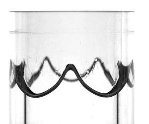
Existing laboratory experiments have revealed that liquid oscillations in Hele-Shaw cells constantly experience an up-and-down driving force with an apparent contact angle $\theta$ constantly changing (Jiang, Perlin & Schultz Reference Jiang, Perlin and Schultz2004). Our experiments are consistent with such evidence. In figure 12, we report seven snapshots, (figure 12a–g), covering one oscillation period, $T$, for the container motion. These snapshots illustrate a zoom of the dynamic meniscus profile and show how the macroscopic contact angle changes in time during the second half of the advancing cycle (figure 12a–e) and the first half of the receding cycle (figure 12f–j), hence highlighting the importance of the out-of-plane meniscus curvature variations. Thus, on the basis of our observations, it seemed appropriate to introduce a contact angle model in the theory to justify this associated additional dissipation, which would be neglected by assuming $M=0$. The model used in this study, and already implemented by Li et al. (Reference Li, Li and Liao2019), is very simple; it assumes the cosine of the dynamic contact angle to linearly depend on the capillary number $Ca$ (Hamraoui et al. Reference Hamraoui, Thuresson, Nylander and Yaminsky2000). Accounting for such a model is shown, both in Li et al. (Reference Li, Li and Liao2019) and in this study, to supplement the theoretical predictions by a sufficient extra dissipation suitable to match experimental measurements.

Figure 12.

Close up of the meniscus dynamics recorded at a driving frequency $1/11.6\ \text {Hz}$ and amplitude $a=1.2\ \text {mm}$ for $m=6$. (a–g) Seven snapshots covering one oscillation period, $T$, for the container motion are illustrated. These snapshots show how the meniscus profile and the macroscopic contact angle change in time during the second half of the advancing cycle and the first half of the receding cycle, hence highlighting the importance of the out-of-plane curvature or capillary effects. See also supplementary movie 6.

This dissipation eventually reduces to a simple damping coefficient $\sigma _{CL}$ as it is of linear nature. A unique constant value of the mobility parameter $M$ is sufficient to fit all our experimental measurements at once, suggesting that the meniscus dynamics is not significantly affected by the evolution of the wave in the azimuthal direction, i.e. by the wavenumber, and $M$ can be seen as an intrinsic property of the liquid–substrate interface.

Several studies have discussed the dependence of the system's dissipation on the substrate material (Huh & Scriven Reference Huh and Scriven1971; Dussan Reference Dussan1979; Cocciaro, Faetti & Festa Reference Cocciaro, Faetti and Festa1993; Ting & Perlin Reference Ting and Perlin1995; Eral, ’t Mannetje & Oh Reference Eral, ’t Mannetje and Oh2013; Viola, Brun & Gallaire Reference Viola, Brun and Gallaire2018; Viola & Gallaire Reference Viola and Gallaire2018; Xia & Steen Reference Xia and Steen2018). These authors, among others, have unveiled and rationalised interesting features such as solid-like friction induced by contact angle hysteresis. This strongly nonlinear contact line behaviour does not seem to be present in our experiments. This can be tentatively explained by looking at figure 13. These snapshots illustrate how the contact line constantly flows over a wetted substrate due to the presence of a stable thin film deposited and alimented at each oscillation cycle. This feature has also been recently described by Dollet, Lorenceau & Gallaire (Reference Dollet, Lorenceau and Gallaire2020), who showed that the relaxation dynamics of liquid oscillation in a U-shaped tube filled with ethanol, due to the presence of a similar thin film, obey an exponential law that can be well-fitted by introducing a simple linear damping, as done in this work.

Figure 13.

These three snapshots correspond to snapshots (b–d) of figure 12 and show, using a different light contrast, how the contact line constantly moves over a wetted substrate due to the presence of a stable thin film deposited and alimented at each cycle.