Firms play a critical role in determining the overall distribution of resources by deciding how to allocate these resources among their constituent business units. Some of these decisions, such as where to build a new plant or what product lines to invest in, can have important long-term consequences. Other decisions are short-run responses to local business cycle shocks. These decisions, particularly when firms are geographically dispersed, can significantly influence the geographic contours of business cycles. During the Great Depression, manufacturing employment was highly synchronized across regions (Rosenbloom and Sundstrom Reference Rosenbloom and Sundstrom1999). Yet markets in many ways were highly fragmented geographically because of, for example, legal limits on bank branching across state lines, raising the question of what drove the synchronization.
We empirically establish the critical role played by firms in generating spatial spillovers of local shocks during the Depression. To motivate our empirical strategy, take the following concrete example: the Alpha Portland Cement Company. One of its nine constituent establishments was located in La Salle, Illinois, about 100 miles from Chicago. In June 1932, Chicago experienced a terrible banking panic. During the week of 20 June alone, 26 Chicago banks failed, and 40 failed during the whole month, even while there was no similar spike in failures at the state or national level. This event would presumably have affected the Alpha establishment located in Illinois directly, for example, by reducing its customers’ access to credit. The question we address empirically is whether other establishments located in places as far away as Alabama and New York that made up the Alpha Portland Cement Company were also affected by this event through their connections to the Illinois establishment.Footnote 1
Consider a firm’s decision to allocate resources across its constituent establishments when facing a working capital constraint,Footnote 2 which limits the total wage bill of a firm to a fraction of total revenue. Revenue earned by different establishments may have different degrees of pledgeability as collateral for working capital loans. This assumption can be motivated by thinking of working capital more broadly as including trade credit extended to local wholesalers. In this way, establishments in a given region might be exposed to changes in the local availability of funding for their wholesalers. Holding fixed the total amount of financial resources available in the case of a binding working capital constraint, a firm’s geographically-dispersed network of establishments is valuable in that it allows the firm to exploit local shocks by transferring (financial) resources between establishments located in different regions.
With this theoretical motivation, we construct an establishment-level dataset of 25 industries from the Census of Manufactures taken in 1929, 1931, 1933, and 1935. These industries represent just under 20 percent of all manufacturing revenue at this time. We link the establishments to their parent firms. We focus on firm networks distributed across space that are part of the same industry, selling products that are (mainly) geographically differentiated.Footnote 3 As an example, the cement industry consists of firms operating geographically dispersed establishments that produce nearly identical physical products, yet these products are spatially differentiated due to high transportation costs.
We exploit the fact that during the Depression, the United States was, in effect, running an experiment on monetary independence. Like the Eurozone today, there were no barriers to trade between regions of the United States, and all regions of the United States used a common currency. Unlike the Eurozone today, which has centralized monetary policymaking at the European Central Bank, the regional Federal Reserve banks before the consolidation of monetary policymaking at the Board of Governors had a degree of autonomy in how they set monetary policy. This autonomy came not just in the form of the discount rate but also in the conditions required for banks to obtain a discount loan. As a consequence of this autonomy, not only did different Federal Reserve banks set different discount rates, with differences of over 200 basis points at certain times during the 1930s, but they also made dramatically different choices in, for example, what they considered good collateral. These differences in policy, which in many cases were ideologically driven, had major impacts on the supply of credit in a local area. To give a few examples, Richardson and Troost (Reference Richardson and Troost2009) show how policy differences between the St. Louis and Atlanta Federal Reserve banks led to dramatic differences in the number of bank failures across the state of Mississippi following the collapse of the bank Caldwell & Co. in November 1930. Jalil (Reference Jalil2014) finds that bank failures were lower in the Atlanta region along its whole border with other Federal Reserve regions in the first years of the Depression. Carlson, Mitchener, and Richardson (Reference Carlson, Mitchener and Richardson2011) highlight another example where the aggressive discount lending actions of the Atlanta Federal Reserve were essential to stopping a panic in Florida in 1929.
The trilemma (or “impossible trinity”) introduced by Robert Mundell and Marcus Fleming implies that, in an environment like the 1930s United States with free capital flows between regions and a single currency, regional interest rate differentials should be arbitraged away by capital or other resources flowing from low-return to high-return areas. The fact that these differentials were (apparently) not arbitraged away motivates our null hypothesis that resources did not flow in response to local shocks between establishments making up the same firm. The trilemma also motivates our level of geographic analysis at the Federal Reserve district level.
A long literature has shown that local monetary and credit shocks had effects on local economic conditions during the Great Depression, for example, Calomiris and Mason (Reference Calomiris and Mason2003); Ziebarth (Reference Ziebarth2013); Lee and Mezzanotti (Reference Lee and Mezzanotti2017); Amir-Ahmadi, Cortes, and Weidenmier (Reference Amir-Ahmadi, Cortes and Weidenmier2021). We extend that literature by showing that these local credit shocks do not just have local effects but also have spillovers on establishments connected through firm networks. Consistent with an interpretation of these credit shocks as relaxing the working capital constraint, an expansion in the supply of credit for a particular establishment has positive effects on employment at that establishment as well as all other establishments that make up the firm, wherever they are located. These results hold for a variety of measures of credit supply, including the regional discount rate, the amount of bills discounted by the regional Fed, and the amount of distressed loans. As an example of the effect size, a one standard deviation increase in the number of banks temporarily suspended in the regions to which an establishment is connected leads to a 7.6 percent decline in employment in our preferred specification.
Given the apparent flows of resources across regions in response to local credit supply shocks, a puzzle then is how the regional Federal Reserve banks were able to maintain a degree of independent monetary policy in the face of a common currency. Moreover, there are other ways that financial resources, in particular, can move between regions besides through networks of establishments. The most obvious other way is through the financial system. Relative to the present day, the 1930s United States banking system was fragmented geographically due to federal limits on between-state branching and, in some states, limits on within-state branching. This resulted in an overwhelming number of banks operating as unit banks seemingly restricted to raising and lending money locally. In reality, the smallest banks in the most far-flung locations had connections to the broader financial system through correspondent connections that allowed them to obtain funding from non-local sources and deploy excess funds outside their local area. As Richardson (Reference Richardson2007) shows, the correspondent network was a major source of instability during the 1930s. In addition, Mitchener and Richardson (Reference Mitchener and Richardson2019) highlight the effects of the pyramidal structure of financial reserves during the 1930s and the effects this structure had on financial instability. What this literature establishes, at a minimum, is that these networks were reallocating financial resources across space in response to local shocks.
Our theoretical framework assumes that a firm’s network of establishments can act as a substitute for the financial network, with firms having the ability to use their internal resources to substitute for breakdowns in the flow of external credit. This view is consistent with work on modern financial crises. For example, Matvos and Seru (Reference Matvos and Seru2014) estimate a structural model to account for how internal capital markets can act as a substitute for external ones. Santioni, Schiantarelli, and Strahan (Reference Santioni, Schiantarelli and Strahan2017) study the value of these networks for Italian firms during the recent Euro crisis, and Almeida, Kim, and Kim (Reference Almeida, Kim and Brian Kim2015) for Korean chaebol in the Asian financial crisis of 1997. In addition, our theoretical model treats each region’s financial system as disconnected from the system in any other region. In our empirical specification, we attempt to control for the possibility that the financial system is connected regionally. In this way, our results do not depend on the model’s assumption of a geographically fragmented financial system.
Besides relating to the literature on the Great Depression, our paper relates to the literature in corporate finance that studies the functioning of firms’ internal capital markets. Theory has identified the costs and benefits of these markets relative to external, arms-length capital markets for financing new projects. For example, Stein (Reference Stein1997) highlights that these markets allow firms to engage in winner-picking of particularly productive projects. Conversely, Scharfstein and Stein (Reference Scharfstein and Stein2000) emphasize the costs of potential rent seeking by managers of the various projects. An ample literature has attempted to empirically identify these costs and benefits (Shin and Stulz Reference Shin and Stulz1998; Lamont Reference Lamont1997; Rajan, Servaes, and Zingales Reference Rajan, Servaes and Zingales2000; Schoar Reference Schoar2002; Maksimovic and Phillips Reference Maksimovic and Phillips2002; Gomes and Livdan Reference Gomes and Livdan2004).Footnote 4
Finally, our paper relates to the recent literature on modern macroeconomic fluctuations that has emphasized the importance of large firms for understanding business cycle fluctuations. For example, Gabaix (Reference Gabaix2011) argues that when the distribution of firm size is fat-tailed, idiosyncratic shocks do not simply average out in the aggregate. A line of papers, including Di Giovanni, Levchenko, and Mejean (Reference Di Giovanni, Levchenko and Mejean2014, Reference Di Giovanni, Levchenko and Mejean2018), has explored this point. Other work, such as Carvalho and Grassi (Reference Carvalho and Grassi2019), has developed business cycle models that incorporate the firm size distribution in a meaningful way. Finally, research has identified ways in which big firms behave differently over the business cycle. For example, Crouzet and Mehrotra (Reference Crouzet and Mehrotra2020) find that large firms are less cyclically sensitive than the rest. They argue that this is not because of the financial strength of large firms, but rather the broad industry scope of these firms, a point similar to one made in Decker, D’Erasmo, and Boedo (Reference Decker, D’Erasmo and Moscoso Boedo2016). Our work makes a parallel point, emphasizing instead the geographic scope of large firms in a historical context.
HISTORICAL BACKGROUND
The formal model in the Online Appendix highlights that for resources to flow across space inside of firms, establishments must be dependent on local credit markets to a certain extent, and there must be differences across space in credit market conditions (in a sense we make precise). If funding of individual establishments within a firm is being done centrally through national credit markets, then local credit conditions should not matter. While we certainly accept that some part of the funding for the largest firms was done through national credit and equity markets, we argue in this section that local credit market conditions still mattered for these firms, by drawing on the history of firm finance and the role played by regional Federal Reserve banks during the Depression.
During this period, goods tended to be sold under the “cash discount open account system” (Willis and Steiner Reference Willis and Steiner1926, p. 214). In this system, a seller (in our case, the manufacturer) quotes terms of sale to a buyer (in our case, the wholesaler). These terms generally include a certain period in which full payment is required and another shorter period (usually 10 days) during which a specified cash discount (say 2 percent) is granted. These terms were usually standard within an industry, though across industries there was considerable variation based on characteristics of the industry, such as the seasonality of demand or perishability of goods. Wholesalers, when not offering cash as payment, would offer paper promising payment at some future date. Manufacturers, accepting that paper, could have it discounted to get cash immediately from a local bank. That paper, in turn, could be rediscounted by the regional Federal Reserve banks to provide cash to the bank itself through the discount window.Footnote 5 In this way, the regional Federal Reserve banks helped to provide credit to support the working capital needs of businesses.
The dominant banking theory of the time distinguished loans for commercial operations, which were eligible for support from Reserve banks through rediscounting, from loans for investment, which were not eligible. Commercial banks were only supposed to be involved in the former, while investment banks were only involved in the latter. Commercial banks often went so far as to conduct annual “clean ups” of their portfolios to show they were not involved in investment lending (White Reference White and Kasuya2003). For a loan to be considered commercial, it needed to either be “employed to acquire readily salable goods” or used “to further some definite stage of production, distribution or manufacture” (Willis and Steiner 1926, p. 152). A loan’s commercial purpose was critical for determining whether it was eligible or acceptable to be rediscounted by the Federal Reserve. While Reserve banks had “discretion in taking the steps necessary to satisfy itself as to eligibility” of a note (Willis and Steiner 1926, p. 178), the criteria for eligibility should “not [be] the character of the borrower’s business but the use of the proceeds of the particular instrument in question” (Willis and Steiner 1926, p. 219). This view emphasized the function (and term) of the paper as the key criterion for whether it was eligible.Footnote 6 For example, the paper of a utility to purchase coal would be eligible, and it should not matter the identity of the utility.
Even on this seemingly straightforward question of whether funds were being used for commercial as opposed to investment purposes, the policies of the Reserve banks allowed for virtually unlimited discretion in practice. Rather than tests based on financial statements for whether banks had used and would use the proceeds of a discount loan for commercial use, instead use was indicated simply by showing “a reasonable excess of quick assets over current liabilities” (Willis and Steiner 1926, p. 206). With the Banking Act of 1933 (also known as the Glass-Steagall Act), Congress ended the figment that discount lending had to be for commercial purposes and granted the Federal Reserve emergency authority to lend to member banks on any high-quality asset. It made this authority permanent with the Banking Act of 1935. At the same time, the Banking Act of 1933 required the Reserve banks to keep themselves apprised of whether loans were being used for improper (i.e., speculative) uses and to take this information into account when deciding whether or not to rediscount (Whitney Reference Whitney1934).
Beyond discretion on whether a discount loan was for the proper use, regional Federal Reserve banks could and did exercise discretion over the strictness of their lending standards. In a 1931 questionnaire, Atlanta and Boston admitted to varying their standards based on the individual circumstances of the borrowers (Whitney Reference Whitney1934). This was partially driven by the fact that the Board of Governors specifically ruled that paper could not be rediscounted “in any case where the ultimate payment of the note is dependent upon the success of the transaction giving rise to the note” (Willis and Steiner 1926, p. 218). In the view of Willis and Steiner (1926, p. 219), this ruling was inconsistent with a definition of eligible paper based solely on its function. As a practical matter, this inconsistency did not matter since the Reserve banks were under no obligation to rediscount all eligible paper. Reserve banks could refuse to rediscount paper on the grounds that the member banks had not conformed to the policies of the Federal Reserve (Whitney Reference Whitney1934). As Willis and Steiner (1926, p. 206) put it, “while some [Reserve banks] are strict, others have taken almost all eligible paper offered them.” One way in which Reserve banks controlled the volume of discount lending was by requiring additional or so-called marginal collateral. For example, through the summer of 1931, the St. Louis Federal Reserve required double collateral that consisted of the eligible paper required by law plus an equal amount of U.S. government securities. As Westerfield (Reference Westerfield1932, p. 48) stated, “in the requirement of additional collateral there [was] no uniformity among the Federal Reserve banks.”
While policies such as requiring marginal collateral seem like somewhat ad hoc ways to control the volume of discount lending, 8 of the 12 Reserve banks considered managing the volume directly through these tools a superior policy to indirectly managing the volume by setting discount rates (Whitney Reference Whitney1934). The Reserve banks felt that member banks did not often pass on changes in the discount rates to customers, and, for that reason, changes in the discount rate did not necessarily have the effects intended by the Reserve banks. This suggests that perhaps a better measure of the stance of monetary policy at the regional level during this period is the total volume of discount loans rather than the discount rate itself.
An important question for us specifically was how the Reserve banks treated paper involving a borrower that was part of a much larger firm, not necessarily headquartered in the region. Our model assumes, in effect, that the Federal Reserve did not treat establishments that were part of the same firm as necessarily identical. It is hard to get a clear answer on whether this was actually the case. For example, the Board “require[d] that the statement of a borrower who has closely affiliated or subsidiary corporations or firms shall be accompanied by separate statements of the latter, unless his own statement clearly indicates that the ‘note is both eligible from a legal standpoint and acceptable from a credit standpoint’” (Willis and Steiner 1926, p. 181). This seems to suggest the regional Feds needed to consider the firm as a whole and not the individual establishment itself. But the same policy of the Board “authorized the Reserve banks to waive the requirement until May 1, 1925, in any case where separate financial statements have not been issued prior thereto” (Willis and Steiner 1926, p. 181), which points in the other direction.
However the regional Reserve banks treated a borrower that was part of a larger firm, it was the case that if local banks were unwilling to accept the paper from a wholesaler for discount, manufacturers ended up being in effect lenders to their wholesalers. In this way, even manufacturers that were part of a larger firm were potentially sensitive to local credit conditions and the decisions made by the regional Federal Reserve banks. In this way, it was not so much the credit quality of the manufacturer that mattered but the quality of their wholesaler.
DATA
We use establishment-level data from the Census of Manufactures (CoM) covering 25 industries taken in 1929, 1931, 1933, and 1935. This data source provides a detailed picture of manufacturing establishments over the course of the first half of the Depression.Footnote 7 While originally collected for various purposes, we would argue that this sample of industries as a whole reflects the broad contours of the manufacturing sector during this period. The sample covers a sizable portion of manufacturing establishments (about 10 percent of the total), wage earners (about 18 percent), and revenue (about 20 percent), all non-trivial fractions.Footnote 8 It contains a variety of types of industries from high-tech ones of the day, such as aircraft and radios, to durable goods producers such as cement and steel, to non-durable good producers, such as ice cream and manufactured ice. Finally, Benguria, Vickers, and Ziebarth (Reference Benguria, Vickers and Ziebarth2020) conduct formal tests comparing the characteristics of industries in the sample to those not included. They find no statistically significant differences in the number of wage earners, revenue, wages, and revenue per worker. They also show that the sample is not tilted toward counties with relatively higher bank failure rates or larger declines in retail sales between 1929 and 1933.
While providing in many respects more detailed information than the modern CoM, this source does have a few important limitations that shape our empirical analysis. First, the CoM in these years lacks information on investment and the value of capital. These pieces of data are available in the modern CoM and the nineteenth-century ones. This limitation prevents us from focusing on these variables as much as the literature on the internal capital markets has. The second major data limitation of the CoM from this period is a dearth of any information on the financial position of the establishments or their parent firms. The CoM provides nothing about outstanding debt, when that debt matures, equity, or surplus held in reserve. This precludes us from examining whether our results differ based on the financial strength of the firms.
Because of these limitations, we will focus on quarterly establishment-level employment as our dependent variable. This is similar to the dependent variable in Giroud and Mueller (Reference Giroud and Mueller2019). The CoM asked for a breakdown of employees into wage and salary earners. As discussed in Vickers and Ziebarth (Reference Vickers, Ziebarth, Diebolt, Michael and London2018), this distinction between salary versus wage earners is similar to the modern CoM distinction between non-production and production workers. For the wage earner category, the CoM furthermore asked for this count at a monthly frequency. We aggregate these monthly counts to the quarter to smooth out some of the high-frequency fluctuations. We will also make use of the information provided on total wages paid over the whole year in weighting establishments within a firm.
Unlike the modern CoM, the Census Bureau at this time did not provide establishment or firm identifiers. This makes it nontrivial to link the same establishment or firm over time. It also makes it difficult to link the group of establishments that make up the same firm. Therefore, we construct establishment and firm links “by hand.” In the case of establishments, we mainly use the address of an establishment, which should remain fixed over time, and to break ties, we use the names of the establishment and its parent firm.Footnote 9 For firm identifiers, we use the name of the parent company listed on the schedules, supplemented with external sources on particular industries. As one small point, a firm is defined as having multiple establishments if, at any point in a year, it has more than one establishment in operation. This status could change from census to census if establishments within a firm open or close between years, but it is fixed within a particular year.
Given the limitations in the linking process, it is important to identify which types of linking errors could bias our results and in which direction. To look ahead, our main regressions will use quarterly variation in employment as the dependent variable and the economic conditions of the regions where other establishments making up the same firm are located as the key independent variable. So an error in linking an establishment within a particular year to its parent firm can potentially generate biases in the regressions. This means that changes in a firm’s name over time will not be problematic since we only need the name to be consistent within a year.Footnote 10 What is potentially problematic are common-sounding firm names that make it difficult for us to tell if two seemingly similar names are actually referring to the same firm. In these cases, the likely linking error is to “overgroup” establishments, creating overly large firms. Errors of this type would make it more difficult for us to identify the effects of firm network linkages since, by assumption, these links do not exist between establishments incorrectly grouped into a firm. To get a sense of the magnitude of the potential bias here, we conduct a placebo test, where we randomly assign establishments to firms and rerun the regressions. We then compare our estimated effect to the counterfactual distribution of estimates.
One limitation of the constructed firm identifiers is that they identify establishments comprising a firm located within a single industry. Because we do not have the whole universe of manufacturing establishments, we are not able to identify establishments owned by a particular firm that fall outside of the industries in our sample. For example, while we have information on establishments that do the final assembly of automobiles, we do not have information on all of the industries that produce inputs into the production of cars (though we have some, like tire producers). At this time, the Ford Motor Company was highly vertically integrated, even attempting to run its own rubber plantation in Brazil (Grandin Reference Grandin2010). All of these other far-flung establishments owned by Ford will not be in our sample. We do not think this lack of information on establishments outside of these industries is necessarily problematic. Even if all of our results focusing on the horizontal allocation of resources are merely reflections of vertical relationships within the firm, it is still the case that firm networks are important. It is just a different type of connection that matters. In any case, understanding the decision of how a firm allocates its resources in the presence of these vertical relationships is interesting in its own right and is something we leave for future work.
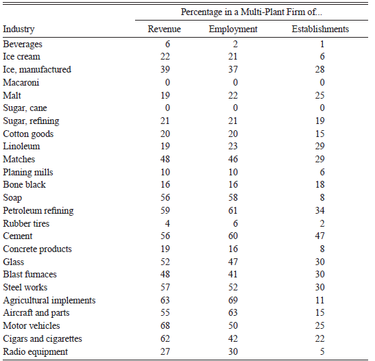
Table 1 reports the importance of multi-establishment firms across our set of industries, pooling all four years. There is considerable variation across the industries in the relative importance of this kind of establishment. The fraction ranges from 2 percent in macaroni to 68 percent in bone black. The range is even larger if we consider revenue or employment percentages that range from 2 percent in macaroni to almost 79 percent in blast furnaces. Finally, we note that, for all industries, this kind of establishment commands more than a proportional share of employment and revenue relative to its share of establishments. This suggests differences, at least in terms of the average size, between these two types of firms.
RELATIVE IMPORTANCE OF MULTI-PLANT ESTABLISHMENTS BY INDUSTRY

Notes: These numbers represent the percentages of industry totals in 1929 for multi-plant establishments. Multi-plant status is defined as whether a firm operates establishments in more than two Federal Reserve districts at any point in 1929.
Sources: The data are from the Census of Manufactures (Vickers and Ziebarth Reference Vickers, Ziebarth, Diebolt, Michael and London2018).
One final point to keep in mind is that the industries differ in their degree of aggregation and whether establishments produce multiple products. The Census Bureau at the time did not use a detailed hierarchical system like SIC codes to organize industries. Some of the industries, such as manufactured ice, macaroni, cement, sugar refining, malt, bone black, and cane sugar, are very narrowly defined and consistent over time, with establishments in these industries tending to make only one product with little product differentiation. On the other hand, the remaining industries are closer to 3-digit SIC codes, with many establishments producing a variety of products. For example, establishments in the agricultural implements industry made reapers, tractors, and thrashers, among other pieces of machinery. In fact, we created the radio industry ourselves by identifying establishments that manufactured radios from the broader industry of producers of electrical equipment. Given that we are not using these industry categories to define, for example, the set of competitors, the broadness of the categories is not particularly problematic. What is potentially problematic is that industry fixed effects will not truly control for what we want them to control for, such as industry-specific seasonal patterns.Footnote 11
Our empirical strategy will use geographic and temporal variation in local credit conditions to identify the effects of firm networks, similar to the work of Giroud and Mueller (Reference Giroud and Mueller2019). Although we have mapped establishments down to the county where they are located, we will work with data on economic conditions at the level of the Federal Reserve region. We choose to work at this geographic level for several reasons. First, there is a tradeoff between geographic detail and sampling frequency. Datasets at a higher frequency tend to be reported at larger geographic units, and we are interested in higher frequency effects of firm networks. Second, there is a risk in using too fine of a geographic unit if that unit does not truly reflect the full extent of an establishment’s product or credit market (though there is also a risk in the other direction of using too coarse of a geographic unit). Third, and most importantly, we think that the Federal Reserve district level is the most interesting level to work at from an economic perspective because of the implications of the trilemma for capital flows.
We consider the effects of several different measures of local credit conditions. First, we examine explicit measures of regional monetary policy, including the discount rate and the amount of bills discounted by the regional Reserve banks. We also examine the effects of measures of private credit indirectly affected by regional monetary policy. These include the quantity of distressed loans, the number of banks terminally and temporarily suspended, deposits in suspended banks, as well as loans in liquidation. All of these measures of private credit were collected from published annual reports of the Federal Reserve and only span the second quarter of 1933, just before the start of the bank holiday. We transform these variables by adding 1, then taking the log to handle the 0s, and finally multiply by minus 1 so that increases in these variables represent increases in the supply of credit.Footnote 12
EMPIRICAL STRATEGY
To measure the spillovers of local economic conditions within the firm, we construct, for each establishment, a measure that summarizes the local conditions of all the other establishments that make up a firm.
An important question in constructing this measure of other conditions is how to weight the local credit conditions at the other establishments that comprise a firm. Following Giroud and Mueller (Reference Giroud and Mueller2019), we construct an employment-weighted average of the economic conditions in regions where other establishments that are part of the same firm are located. This is defined as:

where  it is the local credit supply variable in establishment j’s own region in quarter t, and E
jt–1 is the employment in the previous quarter at establishment j, and the sum is over all establishments in firm f except for establishment i. We use lagged employment to eliminate a simultaneity issue that would arise if we used contemporaneous employment. As a consequence, we effectively drop observations from the first quarter of each year since the biennial nature of the census means we do not have a previous quarter for these establishments. We experiment with different weights to construct the other variable, including weighting by revenue and equally weighting establishments.
Our main specification will focus on the establishments that are part of a firm with operations in multiple geographies. It is the case that the other measure is well-defined even for firms with operations in a single geography. However, in these cases, the other measure will be exactly equal to its own measure. Because of this fact, establishments of this type would not help us identify spillovers, though they would help us identify the effects of the additional controls we include, like industry fixed effects, for example. Nevertheless, we drop these establishments in our main analyses and define a multi-plant (MP) establishment as one that is part of a firm operating in multiple Federal Reserve districts.Footnote 13
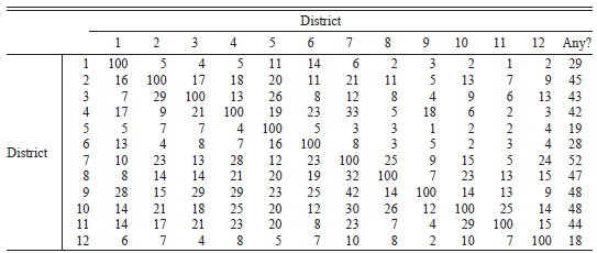
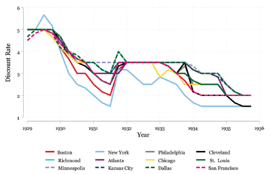
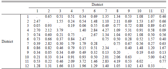
To identify the effect of the other variable, three things need to be true. First, establishments need to be connected across space through firm links. Table 2, which shows the share of establishments that have a within-firm link to an establishment in each of the Federal Reserve regions, demonstrates that these connections in 1929 were substantial.Footnote 14 Note that this matrix does not need to be, and is not, symmetric since the denominator in element (i, j), all establishments located in region i, is different from that of element (j, i), all establishments located in region j. These percentages range from 1 percent to 42 percent of employment. Moreover, the fact that the percentages across a row vary implies that there is also variation in where establishments in a given region have a connection. The last column shows the percentage of employment in a given region that has a connection to any other region. Second, for this strategy to work, it must be the case, as we highlighted earlier, that establishments in a given region are not all connected to the same set of other regions. Third, even with differences across establishments in terms of networks, if there are no differences across regions in terms of economic conditions, then there will be no variation in the other variable. For example, Figure 1 shows the variation for regional discount rates during this period. In the middle of 1931, there was a nearly 200 basis point difference between the largest and smallest discount rates set by the regional Federal Reserves. The New York Fed’s rate was lower than the highest rate by more than 100 basis points for more than a year, starting in early 1930. It is well known that bank failure rates varied enormously across space during the Depression.
CONNECTIONS BETWEEN FEDERAL RESERVE DISTRICTS

Notes: Entry (i, j) is the percentage of establishments located in Federal Reserve district i that are part of a firm with an establishment in Federal Reserve district j. We weight such a connection by the employment of establishments in Federal Reserve district i. Entries on the diagonal will have by construction a value of 100. Rows do not necessarily sum to 100 (even excluding the diagonal element) since an establishment could have connections to multiple Federal Reserve districts. The last column is the percentage of establishments with a connection to any other Federal Reserve district.
Sources: The data are from the Census of Manufactures (Vickers and Ziebarth Reference Vickers, Ziebarth, Diebolt, Michael and London2018).
DISCOUNT RATES BY FEDERAL RESERVE DISTRICT
Notes: This figure plots the average monthly discount rate by quarter across Federal Reserve districts. Not all lines are visible because of the fact that certain regional Federal Reserve Banks sometimes set identical discount rates.
Sources: These data are from the Board of Governors of the Federal Reserve System, Condition of the Federal Reserve Banks, various years.

Letting e it be log quarterly employmentFootnote 15 at establishment i and time t, we estimate the following regression on the set of MP establishments:

Our baseline specification includes fixed effects for county-industry-seasonal trends (County×Quarter×Ind) where Quarter is calendar quarter of the year. We also estimate specifications that add in one-by-one (1) establishment fixed effects; (2) firm fixed effects; and (3) firm revenue interacted with county and quarter. We cluster standard errors at the firm level.Footnote 16
A Placebo Test
In addition to standard errors based on asymptotic theory, we propose the following placebo test akin to a Fisher randomization test to quantify the extent of statistical uncertainty in our estimates. The basic idea of this type of test is to randomly permute treatment and control status and compare the generated density of treatment effects to the estimated one. In our case, we think of the firm network as the treatment, so we randomly permute establishments between firms. The upshot of this test is that it allows for conducting statistical inference without having to rely on asymptotic approximations in the form of the central limit theorem. We interpret the differences between the actual estimate and the distribution of simulated effects as a test of the joint hypothesis that firms are not randomly assembled and that firms do not reallocate resources. If our firm matching was no better than random, then the actual effects should not be much different than the effects based on literally randomly generated sets of firms. If firms did not reallocate resources, then again we would not expect the actual effect to differ from chance.Footnote 17
The test proceeds as follows. First, we randomly assign establishments to firms. Then we calculate the other conditions based on this random assignment and rerun the regression specifications with these randomly created firms. In particular, for a given year and industry, we take as fixed the number of firms and the number of establishments for each firm. Let the set of establishments be denoted by E and the set of firms F. Define the assignment rule f : E → F as the (surjective) function that assigns to each establishment its parent firm. We then draw a random permutation of the establishments σ and apply the rule f◦σ to randomly reassign establishments to firms, maintaining the same distribution of firm sizes within an industry.Footnote 18 With this artificially generated dataset, we rerun our main specifications and collect the point estimates of the own and other effects. We repeat this process 100 times and compare our actual estimate to the distribution of generated effects.
RESULTS
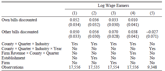
Table 3 shows the results using the quantity of bills discounted.Footnote 19 First, we find that the total volume of bills discounted in an establishment’s own region has a strong positive association with employment across most specifications. For example, Column (1) shows that a 10 percent increase in bills discounted is associated with about a 0.52 percent increase in employment in the baseline specification.Footnote 20 Another way to interpret this coefficient is that the standard deviation over the sample period (at the establishment-level) of the total volume of bills counted is 1.07, so a one standard deviation increase in this variable is associated with a just over 5 percent increase in employment. We do not ascribe a causal interpretation to this estimate. It could be that changes in monetary policy, as reflected in the quantity of bills discounted, are truly driving employment. It could also be that, in line with the Real Bills Doctrine, monetary policy is responding in a pro-cyclical manner to the changes in the demand for credit as proxied by employment. We simply include these estimates to provide a baseline for comparison to the magnitude of the other effects.
EFFECTS OF OWN AND OTHER BILLS DISCOUNTED

Notes: The sample is restricted to establishments that are part of a firm with establishments in multiple districts. These data are at a quarterly frequency at the Federal Reserve district. The base specification includes county by industry by calendar quarter fixed effects. This means we control for industry by county-specific seasonal trends. Standard errors are clustered at the firm-level. The own variable is the value of that variable in an establishment’s own district. The other variable is a weighted average of the variable over all other establishments making up a given firm. Weights are based on employment lagged by one quarter.
Sources: The data for the outcome variable are from the Census of Manufactures (Vickers and Ziebarth Reference Vickers, Ziebarth, Diebolt, Michael and London2018). The data on quantity of bills discounted is from the Board of Governors of the Federal Reserve System, Condition of the Federal Reserve Banks, various years.
Our main result is that the effects of the volume of discount lending by the regional Federal Reserve banks spill over through firms’ establishment networks. Column (1) shows that a 10 percent increase in the quantity of bills discounted in other areas where the establishment’s parent firm is located is associated with a statistically significant increase in employment of 0.5 percent, a non-trivial amount and similar in magnitude to the magnitude of the own effect. Another way to interpret the magnitude of the coefficient is that the effect of a standard deviation increase in the other variable would increase employment by 5.3 percent. These include firm fixed effects, establishment fixed effects, and controls for potential time- and region-varying effects of firm size. As shown in the last column, the result is somewhat sensitive to whether we include a full set of county by time by industry fixed effects.
As we show in the Online Appendix, the randomization tests will be valid under the assumption that networks are randomly constructed (in a certain sense that we make precise). To support this assumption, we now show that the distribution across regions of establishments having a link to region i is the same as the unconditional distribution of establishments across regions, excluding region i. This would provide compelling evidence that the networks were randomly constructed. We have to be careful about the multiple hypothesis problem in this case since we will be making 132 = 12 × 12 – 12 comparisons when a region is defined as a Federal Reserve district. At the 5 percent level, we would expect approximately 7 statistically significant differences even if locations were truly random.
Table 4 shows the distribution of (the absolute value of) t-statistics using the networks from 1929, pooling all industries. We find only mild evidence for non-random networks with about 20 statistically significant t-statistics, which is more than would be expected due to chance. However, the vast majority of differences are quite minor. This result provides support for interpreting the results of randomization tests as a test for the presence of spillovers.
t-STATISTICS COMPARING CONDITIONAL AND MARGINAL DISTRIBUTION OF LOCATIONS

Notes: Entry (i, j) is the absolute value of the t-statistic comparing the fraction of establishments in Federal Reserve district i among establishments with a connection to region j to the unconditional fraction of establishments in Federal Reserve district i. We do not compare region i to itself so diagonal elements are missing. In computing the t-statistic, we treat the unconditional fraction in a district as non-random.
Sources: The data are from the Census of Manufactures (Vickers and Ziebarth Reference Vickers, Ziebarth, Diebolt, Michael and London2018).
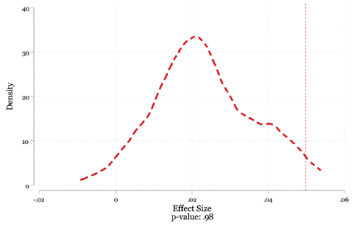
Figure 2 shows the results of the placebo test based on randomly generating firms and re-estimating the regression with total bills discounted. We plot the distribution of simulated other effects as well as the baseline estimate. We find that the actual effect is greater than 98 percent of all the simulated effects and more than 2 times larger than the mode. In the Online Appendix, we show that it is to be expected that the distribution of simulated effects will not be centered at 0.Footnote 21 We take these results as additional evidence of the presence of spillovers.
PLACEBO TEST OF EFFECTS OF OTHER DISCOUNT RATE
Notes: This figure compares the actual estimates from Column (1) in Table 3 denoted by the dashed line with estimates from using randomly generated firms. The distribution is based on 100 simulations. In each simulation, we randomly permute establishments between firms holding fixed the marginal distribution of the number of establishments per firm.
Sources: The data for the outcome variable are from the Census of Manufactures (Vickers and Ziebarth Reference Vickers, Ziebarth, Diebolt, Michael and London2018). The data on the discount rate is from the Board of Governors of the Federal Reserve System, Condition of the Federal Reserve Banks, various years.

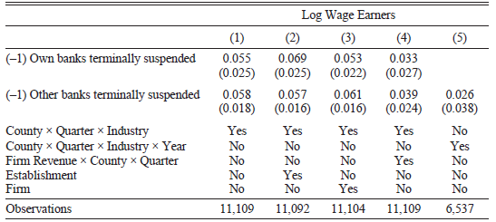
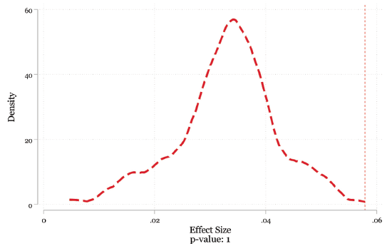
Finally, Table 5 reports the effects of the number of banks that were terminally suspended in the quarter, a (negative) measure of local private credit supply. Remember, we have multiplied these variables by –1 so increases can be interpreted as increases in local credit supply. We again find consistent evidence of positive spillovers. Based on Column (1), a 10 percent increase in the number of banks that were terminally suspended in an establishment’s other region decreases employment by 0.58 percent. A one standard deviation increase in this variable leads to a 7.6 percent decline in employment. The magnitude and statistical significance of these results are qualitatively similar across the different specifications, though the effect is smaller in the fully saturated model. Figure 3 shows the results of the placebo test for this credit supply variable. We find that the actual effect is greater in magnitude than all the simulated effects and nearly double in magnitude than the value of the mode.
EFFECTS OF OWN AND OTHER NUMBER OF BANKS TERMINALLY SUSPENDED

Notes: The sample is restricted to establishments that are part of a firm with establishments in multiple districts. These data are at a quarterly frequency at the Federal Reserve district. The base specification includes county by industry by calendar quarter fixed effects. This means we control for industry by county-specific seasonal trends. Standard errors are clustered at the firm-level. The own variable is the value of that variable in an establishment’s own district. The other variable is a weighted average of the variable over all other establishments making up a given firm. Weights are based on employment lagged by one quarter. The number of banks terminally suspended has been transformed by adding 1 and taking the log, and then multiplying by minus 1. An increase in this credit measure should be interpreted as a decrease in local (private) credit supply.
Sources: The data are from the Census of Manufactures (Vickers and Ziebarth Reference Vickers, Ziebarth, Diebolt, Michael and London2018).
PLACEBO TEST OF EFFECTS OF OTHER NUMBER OF BANKS TERMINALLY SUSPENDED
Notes: This figure compares the actual estimates from Column (1) in Table 5 denoted by the dashed line with estimates from using randomly generated firms. The distribution is based on 100 simulations. In each simulation, we randomly permute establishments between firms holding fixed the marginal distribution of the number of establishments per firm. Because this credit measure has been multiplied by minus 1, an increase in it should be interpreted as an increase in local (private) credit supply.
Sources: The data for the outcome variable are from the Census of Manufactures (Vickers and Ziebarth Reference Vickers, Ziebarth, Diebolt, Michael and London2018). The data on the number of banks terminally suspended are from Federal Deposit Insurance Corporation Data on Banks in the United States, 1920–1936 (ICPSR Study #7).

Taken together, these results provide clear evidence that local credit shocks, both public and private, spilled over inside the firm to establishments not even directly affected, and that might have been geographically quite far away. The existence of these geographic spillovers highlights the critical role played by firms in shaping the geography of the Great Depression. Consider again the example of the banking panic in Chicago in June 1932. Based on our results, not only would the establishments making up Alpha Portland Cement Company located in the Chicagoland area have been negatively affected by the panic, but also the Alpha Portland establishments located in Alabama, over 700 miles away. This spreading out of the effects of the local credit shock does not represent an amplification of the initial shock, but rather a form of risk sharing within a firm. In other words, establishments that are part of geographically dispersed firms are better off than if they were on their own. This is not due to differences in size or access to credit. Instead, the benefit of being part of such a firm is simply due to the presence of this network that allows firms to reallocate resources in response to local shocks without having to deal with the vagaries of external financial markets. For this reason, our results do not help to explain the depth of the Great Depression, but they do help to explain the regional comovement in economic activity.
CONCLUSION
Big firms matter, and they matter in particular for business cycle fluctuations. As one historical example, Hausman (Reference Hausman2016) argues that a shock impacting labor costs, driven by a unionization push at the Big Three automakers, caused the (quite severe) 1937 recession. We studied one dimension of bigness as defined by whether a firm owns multiple establishments and its impacts on the geography of the Depression. To identify the effects of these networks of establishments during the Depression, we collected an establishment-level dataset from the CoM and linked establishments to their parent firms. We found that local credit shocks spilled over between geographically separated establishments constituting the same firm.
Going forward, we see three avenues for future research. First, one salient feature of the Depression was its geographic synchronicity. The obvious, though not entirely satisfying, explanation for this synchronicity is the existence of aggregate shocks. Our results suggest a different explanation in which firm networks spread the effects of local shocks across space, generating the appearance of an aggregate shock. In ongoing work, we are developing an empirical framework that allows us to calculate how much spatial correlation there would have been if there had been no firm networks and how much of the spatial correlation can be attributed to an aggregate shock.
Second, future work is needed to understand the relationship between firm and financial networks. To return to our illustrative example, since many banks in Alabama have correspondents in Chicago, it is possible that the Chicago banking panics impacted the behavior of banks in Alabama. To the extent that this was happening, it could be that the spillover effects we identify are really due to financial rather than firm networks. We think our results would still be just as interesting if this were the explanation, as it would show how these financial networks have real effects, further strengthening the link between finance and the real economy during the Depression. Nevertheless, to fully address this concern would require overlaying these financial networks with these firm networks to separate the effects of each kind of network. In the other direction, our results suggest that perhaps the evidence for the role of financial networks is overstated, and instead, some of what appears to be financial interconnections is actually firm interconnections.
Finally, as we mentioned in the introduction, between the founding of the Federal Reserve System and the consolidation of monetary policymaking at the Board of Governors, the United States conducted an experiment on how much monetary independence is possible in the face of a common currency and no (apparent) capital controls across regions. Apparently, a fair amount of independence was possible, as reflected in large regional differences in discount rates. One explanation for why large gaps in the regional discount rates were able to persist is adjustment costs that prevent the reallocation of capital and economic resources in response to these interest rate differentials. The problem is that we have established in this paper that, in fact, firms did move resources between regions in response to local shocks, and it was not just firms moving resources. So we end up back with the same puzzle: How were the regional Reserve banks able to operate independently in the face of a common currency and relatively free capital flows?