1. Introduction
Oceanographic measurements have widely reported staircase-like structures with regions of nearly constant density in the vertical direction separated by interfaces with a sharp density gradient (Tait & Howe Reference Tait and Howe1968, Reference Tait and Howe1971; Schmitt et al. Reference Schmitt, Perkins, Boyd and Stalcup1987, Reference Schmitt, Ledwell, Montgomery, Polzin and Toole2005; Padman & Dillon Reference Padman and Dillon1989; Muench, Fernando & Stegen Reference Muench, Fernando and Stegen1990; Zodiatis & Gasparini Reference Zodiatis and Gasparini1996; Morell, Corredor & Merryfield Reference Morell, Corredor and Merryfield2006; Timmermans et al. Reference Timmermans, Toole, Krishfield and Winsor2008; Fer et al. Reference Fer, Nandi, Holbrook, Schmitt and Páramo2010; Spear & Thomson Reference Spear and Thomson2012). Such structures are typical of tropical and subtropical regions where warm salty water often overlies cold fresh water and have been ascribed to the presence of salt-finger convection. Indeed, staircases have been observed in the western tropical Atlantic (Schmitt et al. Reference Schmitt, Perkins, Boyd and Stalcup1987, Reference Schmitt, Ledwell, Montgomery, Polzin and Toole2005), Tyrrhenian Sea (Zodiatis & Gasparini Reference Zodiatis and Gasparini1996), and the Mediterranean outflow in the Northeast Atlantic (Tait & Howe Reference Tait and Howe1968, Reference Tait and Howe1971), where conditions for salt-finger convection prevail. These staircases are typically characterised by a large coherence length in the horizontal, much larger than the step height in the vertical. For example, the Caribbean-Sheets and Layers Transect (C-SALT) field programme showed that the well-mixed layers were 5–30 m thick and laterally coherent over scales of 200–400 km (Schmitt et al. Reference Schmitt, Perkins, Boyd and Stalcup1987). The presence of staircases also enhances the tracer mixing rate. For example, the North Atlantic Tracer Release Experiment (NATRE) (Schmitt et al. Reference Schmitt, Ledwell, Montgomery, Polzin and Toole2005) revealed a mixing rate in the western tropical Atlantic five times larger than that in the eastern subtropical Atlantic. Spontaneous formation of staircases has also been observed in idealised laboratory experiments (Linden Reference Linden1978; Krishnamurti Reference Krishnamurti2003, Reference Krishnamurti2009) and direct numerical simulations (DNS) (Piacsek & Toomre Reference Piacsek and Toomre1980; Radko Reference Radko2003, Reference Radko2005; Stellmach et al. Reference Stellmach, Traxler, Garaud, Brummell and Radko2011; Yang et al. Reference Yang, Chen, Verzicco and Lohse2020).
Understanding the origin of spontaneous staircase formation is important for parameterisation and accurate modelling of oceanographic processes. Various mechanisms for staircase formation have been proposed (Radko Reference Radko2013, § 8). The collective instability mechanism (Stern Reference Stern1969; Holyer Reference Holyer1981) identifies conditions for the formation of a staircase based on the instability of the salt-finger field to internal gravity waves, but requires a closure model for the Reynolds stress and the temperature and salinity fluxes based on laboratory measurement and ocean observation. The onset of staircase formation is also predicted by models with negative density diffusion (Phillips Reference Phillips1972; Posmentier Reference Posmentier1977). The related  $\gamma$-instability of Radko (Reference Radko2003) requires a parameterisation of the Nusselt number and the flux ratio but shows good agreement with 2-D and 3-D DNS of salt-finger convection (Radko Reference Radko2003; Stellmach et al. Reference Stellmach, Traxler, Garaud, Brummell and Radko2011). However, these predictions generally only focus on the onset of a large-scale instability suggesting the appearance of a staircase, but do not provide a detailed profile of the final staircase or its parameter dependence. In this connection the model of Balmforth, Llewellyn Smith & Young (Reference Balmforth, Llewellyn Smith and Young1998) is of particular interest. The model parametrises the coupling between buoyancy flux and local turbulent kinetic energy but succeeds in generating robust staircases. Nevertheless, the use of closure models employed in all these predictions results in uncertainty in the applicable parameter regime.
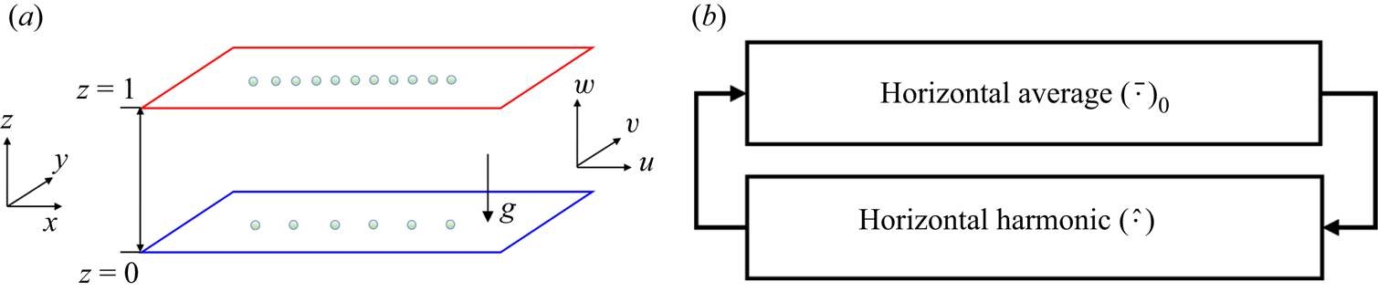
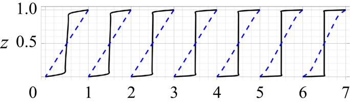
This work aims to discuss an alternative mechanism for spontaneous staircase formation from a bifurcation theory point of view (figure 1), focusing on the computation of strongly nonlinear staircase-like solutions and analysing their stability. Bifurcation analysis has been widely employed to provide insight into pattern formation in fluid dynamics (Crawford & Knobloch Reference Crawford and Knobloch1991). For example, a secondary bifurcation of steady convection rolls in Rayleigh–Bénard convection to tilted rolls was shown to be accompanied by the generation of large-scale shear (Howard & Krishnamurti Reference Howard and Krishnamurti1986; Rucklidge & Matthews Reference Rucklidge and Matthews1996), resembling both experimental observation (Krishnamurti & Howard Reference Krishnamurti and Howard1981) and DNS (Goluskin et al. Reference Goluskin, Johnston, Flierl and Spiegel2014). A sequence of local and global bifurcations of such tilted convection cells in magnetoconvection was shown to lead to a pulsating wave characterised by periodic reversals in the direction of the tilt and the accompanying large-scale shear (Matthews et al. Reference Matthews, Proctor, Rucklidge and Weiss1993; Proctor & Weiss Reference Proctor and Weiss1993; Proctor et al. Reference Proctor, Weiss, Brownjohn and Hurlburt1994; Rucklidge & Matthews Reference Rucklidge and Matthews1996). In the diffusive configuration in which cold fresh water overlies warm salty water, a similar analysis found stable travelling waves near onset (Knobloch et al. Reference Knobloch, Deane, Toomre and Moore1986) and provided insight into the transition to chaos (Knobloch, Proctor & Weiss Reference Knobloch, Proctor and Weiss1992). Such chaotic or even fully developed turbulent states generally visit neighbourhoods of (unstable) steady, periodic or travelling wave solutions, and these visits leave an imprint on the flow statistics; see, e.g. Kawahara & Kida (Reference Kawahara and Kida2001), van Veen, Kida & Kawahara (Reference van Veen, Kida and Kawahara2006) and the reviews by Kawahara, Uhlmann & van Veen (Reference Kawahara, Uhlmann and van Veen2012) and Graham & Floryan (Reference Graham and Floryan2021).
(a) The salt-finger convection set-up. The red colour indicates a hot plate while the blue colour suggests a cold plate. The number of circles on top and bottom plates suggests the salinity at the top is higher than at the bottom. (b) Nonlinear interaction within the single-mode equations (2.7): horizontal averages  $(\,\bar {\cdot }\,)_0$ influence the horizontal harmonics
 $(\,\hat {\cdot }\,)$ through (2.7a)–(2.7d), whereas the horizontal harmonics
 $(\,\hat {\cdot }\,)$ contribute to the horizontal averages
 $(\,\bar {\cdot }\,)_0$ through (2.7e)–(2.7g).

This work focuses on vertically confined salt-finger convection in order to understand the interior between two well-mixed layers. Although stress-free velocity boundary conditions are suitable for understanding oceanographic scenarios, no-slip boundary conditions are more relevant to laboratory experiments (Hage & Tilgner Reference Hage and Tilgner2010). A wide range of bifurcation analyses of related problems have been performed on vertically confined systems with different boundary conditions including Rayleigh–Bénard convection. In the salt-finger case the fluxes generated in a vertically confined system agree quantitatively with those obtained in a vertically periodic domain when normalised by the bulk conductive fluxes (Li & Yang Reference Li and Yang2022) despite the elimination of the elevator mode that is present in vertically periodic domains; see, e.g. Stern (Reference Stern1969), Holyer (Reference Holyer1984) and Radko (Reference Radko2013, § 2.1).
In order to facilitate bifurcation analysis, we focus here on the single-mode equations obtained from a severely truncated Fourier expansion in the horizontal. Such single-mode equations reduce the two (or three) spatial dimensions in the primitive equations to one vertical dimension, with the dependence on the horizontal direction parameterised by a single assumed horizontal wavenumber. Such a truncation may provide insight into salt-finger convection as the underlying flow structures are dominated by well-organised columnar structures; see, e.g. the visualisation of confined salt-finger convection by Yang, Verzicco & Lohse (Reference Yang, Verzicco and Lohse2016a, figure 7). This single-mode formulation also explicitly isolates and describes the interaction between horizontally averaged modes (corresponding to the staircase or large-scale shear) and the horizontal harmonics (corresponding to fingers), in the spirit of mean-field theory; see, e.g. Garaud (Reference Garaud2018, § 3.2.1). Moreover, the single-mode equations do not require any closure assumptions for the Reynolds stress and the temperature and salinity fluxes to parametrise the feedback between the fluctuations and horizontally averaged quantities, while preserving the nonlinear interaction between them; see figure 1(b).
Single-mode equations have been widely employed to provide insight into related problems. For example, single-mode solutions (also called ‘single- $\alpha$ mean-field theory’) for Rayleigh–Bénard convection with stress-free boundary conditions have been shown to reproduce the mean temperature profile expected at high Rayleigh numbers (Herring Reference Herring1963). For no-slip boundaries at high Prandtl numbers, the Nusselt number predicted from this framework is within 20 % of the experimental value and the root-mean-square velocity and temperature fluctuations also resemble the profiles seen in experimental measurements (Herring Reference Herring1964). Single-mode theory has since been extended to the time-dependent problem (Elder Reference Elder1969) and to more general planforms (e.g. hexagonal) (Gough, Spiegel & Toomre Reference Gough, Spiegel and Toomre1975; Toomre, Gough & Spiegel Reference Toomre, Gough and Spiegel1977), showing qualitative agreement with experimental results. The vertical vorticity mode was included within the single-mode equations with hexagon planform by Lopez & Murphy (Reference Lopez and Murphy1983), Murphy & Lopez (Reference Murphy and Lopez1984), Massaguer & Mercader (Reference Massaguer and Mercader1988), Massaguer, Mercader & Net (Reference Massaguer, Mercader and Net1990) and is excited beyond a secondary bifurcation of convection rolls. Such single-mode equations have also proved to provide insight into many other problems including rotating convection (Baker & Spiegel Reference Baker and Spiegel1975), plane Poiseuille flow (Zahn et al. Reference Zahn, Toomre, Spiegel and Gough1974) and double-diffusive convection (Gough & Toomre Reference Gough and Toomre1982; Paparella & Spiegel Reference Paparella and Spiegel1999; Paparella, Spiegel & Talon Reference Paparella, Spiegel and Talon2002). In particular, DNS of single-mode solutions of salt-finger convection show that fingers can tilt leading to the spontaneous formation of large-scale shear, which may be steady or oscillate, together with a staircase-like profile in the horizontally averaged salinity (Paparella Reference Paparella1997; Paparella & Spiegel Reference Paparella and Spiegel1999). Moreover, in certain asymptotic regimes single-mode solutions may be exact; see, e.g. the high wavenumber (tall and thin) limit of Rayleigh–Bénard convection (Blennerhassett & Bassom Reference Blennerhassett and Bassom1994), convection in a porous medium (Lewis, Rees & Bassom Reference Lewis, Rees and Bassom1997) or salt-finger convection (Proctor & Holyer Reference Proctor and Holyer1986). Such high wavenumber regimes are naturally achieved in convection with strong restraints such as rapid rotation (Julien & Knobloch Reference Julien and Knobloch1997) or strong magnetic field (Julien, Knobloch & Tobias Reference Julien, Knobloch and Tobias1999; Calkins et al. Reference Calkins, Julien, Tobias, Aurnou and Marti2016; Plumley et al. Reference Plumley, Calkins, Julien and Tobias2018) and the resulting exact single-mode equations have proved immensely useful for understanding these systems; see the review by Julien & Knobloch (Reference Julien and Knobloch2007).
This work performs bifurcation analysis of vertically confined salt-finger convection using single-mode equations. The resulting equations are solved for the vertical structure of the solutions as a function of the density ratio, the Prandtl number and the assumed horizontal wavenumber. We fix the diffusivity ratio and thermal Rayleigh number and focus almost exclusively on no-slip velocity boundary conditions. We found staircase-like solutions with one (S1), two (S2) and three (S3) steps in the mean salinity profile in the vertical direction, all of which bifurcate from the trivial solution. In each case salinity gradients are expelled from regions of closed streamlines, leading to a mixed layer. Secondary bifurcations of S1 lead to either tilted fingers (TF1) or travelling waves (TW1), both of which break the horizontal reflection symmetry via the spontaneous formation of large-scale shear. Secondary bifurcations of S2 and S3 lead to asymmetric solutions (A2 and A3) that spontaneously break midplane reflection symmetry.
The stability and accuracy of the single-mode solutions are further analysed with the assistance of 2-D DNS. Near onset, the one-layer solution S1 is stable and corresponds to maximum salinity transport among all known solutions, a fact that is consistent with the prediction of the ‘relative stability’ criterion (Malkus & Veronis Reference Malkus and Veronis1958). The associated Sherwood number (or salinity Nusselt number) near the high wavenumber onset is in excellent agreement with DNS in small horizontal domains. In large domains the DNS reveals a tendency to revert to the characteristic finger scale but the wavenumber of the final state exhibits a strong dependence on initial conditions (if the final state is steady) or the state may remain chaotic. The S2, S3, A2 and A3 solutions are all unstable within the explored parameter regimes, but may be imprinted on the statistics of the chaotic state. At lower density ratios, the S1, S2 and S3 salinity profiles all sharpen and the large-scale shear and tilt angle of the TF1 state increases. The TW1 solutions are also present in this regime, whereas low Prandtl numbers favour direction-reversing tilted fingers (RTF), a state in which the tilt direction and associated large-scale shear reverse periodically as in the pulsating wave.
The remainder of this paper is organised as follows. Section 2 describes the problem set-up and the formulation of the single-mode equations. The equations are solved using numerical continuation and their stability properties are established for Prandtl number  $Pr=7$ in § 3. The tilted finger and travelling wave states are analysed for
 $Pr=0.05$ in § 4. The paper concludes with a brief summary and discussion in § 5.
2. Single-mode equations for confined salt-finger convection
We consider a fluid between two infinitely long parallel plates separated by a distance  $h$. The temperature and salinity at these two plates are maintained at constant values with the top plate maintained at a higher temperature and salinity, as illustrated in figure 1(a). The equation of state
 $(\rho _*-\rho _{r*})/\rho _{r*}=-\alpha (T_*-T_{r*})+\beta (S_*-S_{r*})$ is linear, with constant expansion/contraction coefficients
 $\alpha$,
 $\beta$ and reference density, temperature and salinity
 $\rho _{r*}$,
 $T_{r*}$ and
 $S_{r*}$, respectively. The subscript
 $*$ denotes a dimensional variable. In the following we non-dimensionalise the temperature
 $T_*$ by the temperature difference between the top and bottom layer,
 $T=T_*/\Delta T$ (
 $\Delta T>0$), and likewise for the salinity
 $S_*$,
 $S=S_*/\Delta S$ (
 $\Delta S>0$). Spatial variables are non-dimensionalised by the height
 $h$ of the layer whereas time and velocity are non-dimensionalised using the thermal diffusion time
 $h^2/\kappa _T$ and the corresponding speed
 $\kappa _T/h$, respectively. Here
 $\kappa _T$ is the thermal diffusivity. We decompose the temperature and salinity into a linear base state and deviation,
 \begin{equation} T=z+{\tilde{T}},\quad S=z+{\tilde{S}}, \end{equation}
and introduce the velocity field  $\boldsymbol {u}:=(u,v,w)$ in Cartesian coordinates
 $(x,y,z)$ with
 $z$ in the upward vertical direction. Dropping the tildes and assuming the Boussinesq approximation the system is governed by
 $$\begin{gather} \partial_t\boldsymbol{u}+\boldsymbol{u}\boldsymbol{\cdot} \boldsymbol{\nabla}\boldsymbol{u}= Pr\nabla^2\boldsymbol{u}-\boldsymbol{\nabla} p+Pr Ra_T\left( T-R_\rho^{{-}1} S\right)\boldsymbol{e}_z, \end{gather}$$
 $$\begin{gather}\boldsymbol{\nabla}\boldsymbol{\cdot} \boldsymbol{u}=0, \end{gather}$$
 $$\begin{gather}\partial_t T+\boldsymbol{u}\boldsymbol{\cdot} \boldsymbol{\nabla}T+w= \nabla^2 T, \end{gather}$$
 $$\begin{gather}\partial_t S+\boldsymbol{u}\boldsymbol{\cdot} \boldsymbol{\nabla}S+w=\tau \nabla^2 S. \end{gather}$$
Here  $p$ is the dimensionless pressure
 $p=p_*h^2/\kappa _T^2 \rho _{r*}$ whereas
 $\boldsymbol {e}_z$ in (2.2a) is the unit vector in the vertical direction associated with buoyancy. The governing parameters include the Prandtl number, the diffusivity ratio, the density ratio and the thermal Rayleigh number defined by
 \begin{equation} Pr:=\frac{\nu}{\kappa_T},\quad \tau:=\frac{\kappa_S}{\kappa_T},\quad R_\rho:=\frac{\alpha \Delta T}{\beta \Delta S},\quad Ra_T:=\frac{ g \alpha \Delta T h^3}{\kappa_T\nu }, \end{equation}
where  $\nu$ is the viscosity and
 $\kappa _S$ is the salinity diffusivity.
We impose constant temperature and salinity as boundary conditions at the top and the bottom plates,
 $$\begin{gather} T(x,y,z=0,t)=T(x,y,z=1,t)=0, \end{gather}$$
 $$\begin{gather}S(x,y,z=0,t)=S(x,y,z=1,t)=0, \end{gather}$$
whereas for the velocity we adopt no-slip boundary conditions:
 \begin{equation} \boldsymbol{u}(x,y,z=0,t)=\boldsymbol{u}(x,y,z=1,t)=0.\end{equation}
Periodic boundary conditions in the horizontal are imposed on all variables.
We next formulate single-mode equations following the procedure in Herring (Reference Herring1963, Reference Herring1964), Gough et al. (Reference Gough, Spiegel and Toomre1975), Gough & Toomre (Reference Gough and Toomre1982), Paparella & Spiegel (Reference Paparella and Spiegel1999) and Paparella et al. (Reference Paparella, Spiegel and Talon2002). The single-mode ansatz is
 $$\begin{gather} S(x,y,z,t)=\bar{S}_0(z,t)+\hat{S}(z,t)\exp({\text{i}(k_x x+k_y y)})+{\rm c.c.}, \end{gather}$$
 $$\begin{gather}T(x,y,z,t)=\bar{T}_0(z,t)+\hat{T}(z,t)\exp({\text{i}(k_x x+k_y y)})+{\rm c.c.}, \end{gather}$$
 $$\begin{gather}\boldsymbol{u}(x,y,z,t)=\bar{U}_0(z,t)\boldsymbol{e}_x+\hat{\boldsymbol{u}}(z,t) \exp({\text{i}(k_x x+k_y y)})+{\rm c.c.}, \end{gather}$$
 $$\begin{gather}p(x,y,z,t)=\bar{P}_0(z,t)+\hat{p}(z,t)\exp({\text{i}(k_x x+k_y y)})+{\rm c.c.}, \end{gather}$$
where c.c. denotes the complex conjugate. Equation (2.6a) decomposes the departure of the salinity from the linear profile into a horizontally averaged quantity  $\bar {S}_0(z,t)$ and a single harmonic in the horizontal direction associated with the wavenumber pair
 $(k_x,k_y)$ and characterised by the complex amplitude
 $\hat {S}(z,t)$. The temperature is decomposed similarly. To allow for mean flow in the horizontal we decompose the velocity into a large-scale shear
 $\bar {U}_0(z,t)\boldsymbol {e}_x$ and a harmonic associated with the same wavenumber pair
 $(k_x,k_y)$ as in (2.6c), assuming that the large-scale shear
 $\bar {U}_0$ is generated in the
 $x$-direction. This is appropriate in a 2-D configuration, but in three dimensions the large-scale shear can be oriented in principle in any horizontal direction, a possibility that is left for future study. The horizontally averaged vertical velocity is zero based on the continuity equation (2.2b) and the boundary conditions
 $w(z=0)=w(z=1)=0$. The horizontally averaged quantities
 $(\,\bar {\cdot }\,)_0$ are real and the amplitudes of the horizontal harmonics
 $(\,\hat {\cdot }\,)$ are in general complex. Equations (2.6) assume a horizontal planform in the form of square or rectangular cells, an assumption that also includes 2-D rolls when
 $k_y=0$. Other planforms such as hexagons generate additional self-interaction terms in the single-mode equations (Gough et al. Reference Gough, Spiegel and Toomre1975) and we leave this extension to future work.
We now substitute (2.6) into the governing equations (2.2), dropping all harmonics beyond the first, and balance separately the horizontally averaged components and the harmonic components. We eliminate the horizontally averaged pressure via  $-\partial _z \bar {P}_0+PrRa_T(\bar {T}_0-R_\rho ^{-1}\bar {S}_0)=0$ and eliminate the harmonic component of the pressure using the continuity equation (2.2b). The resulting single-mode equations can then be expressed in terms of the vertical velocity
 $w$ and vertical vorticity
 $\zeta :=\partial _y u-\partial _x v$:
 $$\begin{gather} \partial_t\hat{\nabla}^2\hat{w}+\text{i}k_x\bar{U}_0\hat{\nabla}^2\hat{w}- \text{i}k_x\bar{U}_0''\hat{w}=Pr\hat{\nabla}^4\hat{w}+Pr\hat{\nabla}_\perp^2 Ra_T(\hat{T}-R_\rho^{{-}1} \hat{S}), \end{gather}$$
 $$\begin{gather}\partial_t \hat{\zeta}+\text{i}k_x \bar{U}_0 \hat{\zeta}+\text{i}k_y \bar{U}_0'\hat{w}= Pr\hat{\nabla}^2 \hat{\zeta}, \end{gather}$$
 $$\begin{gather}\partial_t\hat{T}+\text{i}k_x\bar{U}_0\hat{T}+\hat{w}\partial_z \bar{T}_0+\hat{w}= \hat{\nabla}^2\hat{T}, \end{gather}$$
 $$\begin{gather}\partial_t\hat{S}+\text{i}k_x\bar{U}_0\hat{S}+\hat{w}\partial_z \bar{S}_0+\hat{w}= \tau \hat{\nabla}^2\hat{S}, \end{gather}$$
 $$\begin{gather}\partial_t \bar{U}_0+\partial_z(\hat{w}^*\hat{u}+\hat{w}\hat{u}^*)= Pr\partial_z^2\bar{U}_0, \end{gather}$$
 $$\begin{gather}\partial_t \bar{T}_0+\partial_z(\hat{w}^*\hat{T}+\hat{w}\hat{T}^*)= \partial_z^2 \bar{T}_0, \end{gather}$$
 $$\begin{gather}\partial_t \bar{S}_0+\partial_z(\hat{w}^*\hat{S}+\hat{w}\hat{S}^*)= \tau \partial_z^2 \bar{S}_0, \end{gather}$$
 $$\begin{gather}\hat{u}=\frac{\text{i}k_x\partial_z \hat{w}}{k_x^2+k_y^2}-\frac{\text{i}k_y\hat{\zeta}}{k_x^2+k_y^2},\qquad\hat{v}=\frac{\text{i}k_y \partial_z \hat{w}}{k_x^2+k_y^2}+\frac{\text{i}k_x \hat{\zeta}}{k_x^2+k_y^2}, \end{gather}$$
where the superscript  $^*$ denotes a complex conjugate and
 $\hat {\nabla }^2:=\partial _z^2-k_x^2-k_y^2$,
 $\hat {\nabla}^2_\perp :=-k_x^2-k_y^2$,
 $\hat {\nabla }^4:=\partial _z^4-2(k_x^2+k_y^2)\partial _z^2+(k_x^2+k_y^2)^2$,
 $\bar {U}_0':=\partial _z \bar {U}_0$ and
 $\bar {U}_0'':=\partial _z^2 \bar {U}_0$. The corresponding boundary conditions for the salinity and temperature are:
 $$\begin{gather} \hat{S}(z=0,t)=\hat{S}(z=1,t)=\hat{T}(z=0,t)=\hat{T}(z=1,t) \end{gather}$$
 $$\begin{gather}=\bar{S}_0(z=0,t)=\bar{S}_0(z=1,t)=\bar{T}_0(z=0,t)=\bar{T}_0(z=1,t)=0, \end{gather}$$
whereas the no-slip boundary conditions in (2.5) correspond to
 $$\begin{gather} \hat{w}(z=0,t)=\hat{w}(z=1,t)=\partial_z\hat{w}(z=0,t)=\partial_z\hat{w}(z=1,t) \end{gather}$$
 $$\begin{gather}=\hat{\zeta}(z=0,t)=\hat{\zeta}(z=1,t)=\bar{U}_0(z=0,t)=\bar{U}_0(z=1,t)=0. \end{gather}$$
Equations (2.7a)–(2.7d) are the governing equation for the first harmonic in the presence of the large-scale fields  $\bar {U}_0$,
 $\bar {T}_0$ and
 $\bar {S}_0$. In particular, (2.7a) is the Orr–Sommerfeld equation modified by an additional buoyancy term, whereas (2.7b) is known as the Squire equation for the vertical vorticity (Schmid & Henningson Reference Schmid and Henningson2012). Note that the large-scale shear
 $\bar {U}_0$ is self-induced (i.e. a variable to be solved for) instead of an imposed background shear. Thus, the terms involving
 $\bar {U}_0$ in (2.7a)–(2.7d) are also nonlinear. The remaining equations (2.7e)–(2.7g) are the governing equations for the horizontally averaged quantities, distorted by the harmonic fluctuations. The resulting nonlinear interaction between horizontally averaged quantities and horizontal harmonics is summarised schematically in figure 1(b). Equation (2.7h) is used to obtain the horizontal velocity
 $\hat {u}$ from the
 $\hat {w}$ and
 $\hat {\zeta }$ required for the computation of the Reynolds stress in (2.7e).
Similar single-mode equations were previously used to study double-diffusive convection focusing on the diffusive regime (see e.g. Gough & Toomre Reference Gough and Toomre1982, (3.7)–(3.11)), but did not include the coupling to the large-scale shear  $\bar {U}_0$. A numerical simulation of the above single-mode equations in a 2-D configuration (i.e. with
 $k_y=0, \hat{v}=0$) and stress-free boundary conditions was employed to study double-diffusive convection in both the fingering regime (Paparella & Spiegel Reference Paparella and Spiegel1999) and the diffusive regime (Paparella et al. Reference Paparella, Spiegel and Talon2002).
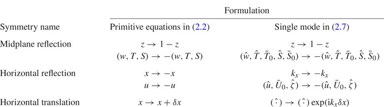
Here we focus on the bifurcation properties of the single-mode equations (2.7). These reflect the symmetries of the primitive equations (2.2), including midplane reflection, horizontal reflection and horizontal translation, as summarised in table 1. In the following, we use the numerical software pde2path (Uecker, Wetzel & Rademacher Reference Uecker, Wetzel and Rademacher2014; Uecker Reference Uecker2021a) to compute strongly nonlinear solutions of the above problem as a function of the system parameters and analyse their stability. The vertical direction is discretised using the Chebyshev collocation method with derivatives calculated using the Chebyshev differentiation matrix (Weideman & Reddy Reference Weideman and Reddy2000) implemented following Uecker (Reference Uecker2021b). The number of grid points used, including the boundary, ranges from  $N_z=65$ for results at
 $R_\rho =40$ to
 $N_z=257$ for results at
 $R_\rho =2$; our continuation in
 $R_\rho$ also uses
 $N_z=257$ grid points. The solutions are obtained by arclength continuation including prediction and Newton-correction steps from a given solution profile at a nearby parameter; see Uecker et al. (Reference Uecker, Wetzel and Rademacher2014, § 2.1) and Uecker (Reference Uecker2021a, § 3.1). The tolerance of the maximal absolute value of the residue at each vertical location (
 $L_\infty$ norm) is set to
 $10^{-6}$.

The presence of horizontal translation symmetry within the single-mode equations requires a phase condition whenever  $k_x\neq 0$ in order to fix the solution phase and obtain a unique solution. The implementation of this condition following Rademacher & Uecker (Reference Rademacher and Uecker2017) requires the predictor
 $\boldsymbol {\psi }(z,t)$ from a solution
 $\boldsymbol {\psi }_{{old}}(z,t)$ to be orthogonal to
 $\text {i}\boldsymbol {\psi }_{{old}}(z,t)$:
 \begin{equation} \int_{0}^1 \text{i}\boldsymbol{\psi}_{{old}}(z,t)[\boldsymbol{\psi}(z,t)-\boldsymbol{\psi}_{{old}}(z,t)]^* \,{\rm d}z=0,\end{equation}
where
 \begin{equation} \boldsymbol{\psi}(z,t):=[\hat{w}(z,t),\hat{\zeta}(z,t),\hat{T}(z,t),\hat{S}(z,t)]^{\text{T}}. \end{equation}
The horizontally averaged modes are not involved in setting the phase.
To compute a steady nonlinear wave travelling in the  $x$ direction with speed
 $c$ we write (2.7a)–(2.7d) in the comoving frame,
 $$\begin{gather} \partial_t\hat{\nabla}^2\hat{w}+\text{i}k_x\bar{U}_0\hat{\nabla}^2\hat{w}- \text{i}ck_x \hat{\nabla}^2 \hat{w}-\text{i}k_x\bar{U}_0''\hat{w}= Pr\hat{\nabla}^4\hat{w}+Pr\hat{\nabla}_\perp^2 Ra_T(\hat{T}-R_\rho^{{-}1}\hat{S}), \end{gather}$$
 $$\begin{gather}\partial_t \hat{\zeta}+\text{i}k_x \bar{U}_0 \hat{\zeta}-\text{i}ck_x\hat{\zeta}+\text{i}k_y \bar{U}_0'\hat{w}=Pr\hat{\nabla}^2 \hat{\zeta}, \end{gather}$$
 $$\begin{gather}\partial_t\hat{T}+\text{i}k_x\bar{U}_0\hat{T}-\text{i}ck_x\hat{T}+\hat{w}\partial_z \bar{T}_0+\hat{w}= \hat{\nabla}^2\hat{T}, \end{gather}$$
 $$\begin{gather}\partial_t\hat{S}+\text{i}k_x\bar{U}_0\hat{S}-\text{i}ck_x \hat{S}+\hat{w}\partial_z \bar{S}_0+\hat{w}=\tau \hat{\nabla}^2\hat{S}, \end{gather}$$
and set the time derivatives in these equations and in (2.7e)–(2.7g) to zero. With the phase condition (2.10) the resulting problem has a unique nonlinear eigenvalue  $c$ and associated solution profile. Both are updated at each step of the continuation procedure. Steady solutions have
 $c=0$, typically within the order of machine precision.
The stability of each solution is examined via the eigenvalues of the associated Jacobian matrix. The eigenvalue computation uses the eigs command in MATLAB to compute a subset of the eigenvalues. We compute 40 eigenvalues near 0 to identify bifurcation points and also compute 1 eigenvalue near 100 to help identify unstable eigenvalues; see the discussion in Uecker (Reference Uecker2021a, Remark 3.12(b)). For validation we reproduced the results for single-mode equations for Rayleigh–Bénard convection (Herring Reference Herring1963, Reference Herring1964; Toomre et al. Reference Toomre, Gough and Spiegel1977), as well as the high-wavenumber asymptotic single-mode equations for this problem (Bassom & Zhang Reference Bassom and Zhang1994, § 3) and for porous medium convection (Lewis et al. Reference Lewis, Rees and Bassom1997, § 3). Selected solution profiles and eigenvalues obtained from pde2path were also validated against the results obtained from the nonlinear boundary value problem (NLBVP) and eigenvalue problem (EVP) solvers in Dedalus (Burns et al. Reference Burns, Vasil, Oishi, Lecoanet and Brown2020), where the EVP solver is chosen to return the full set of eigenvalues. Finally, selected predictions from the bifurcation diagram and stability properties (figure 20a) were also validated against DNS (initial value problem solver) of the single-mode equations (2.7) using Dedalus (Burns et al. Reference Burns, Vasil, Oishi, Lecoanet and Brown2020).
We also performed 2-D DNS of the primitive equations (2.2) using Dedalus (Burns et al. Reference Burns, Vasil, Oishi, Lecoanet and Brown2020) to further analyse the accuracy and stability of the solutions obtained from the bifurcation analysis of the single-mode equations. We focus on 2-D domains with periodic boundary conditions in the horizontal and the no-slip boundary conditions (2.5) in the vertical direction. We use a Chebyshev spectral method in the vertical direction with  $N_z=128$ grid points with a Fourier spectral method in the horizontal direction with
 $N_x=128$ and a dealiasing scaling factor 3/2. To check the accuracy we doubled the number of grid points in both
 $x$ and
 $z$ directions for selected results and confirmed that the resulting Sherwood number
 $Sh$ in figure 18 (steady rolls resembling the S1 solution) does not change up to eight decimal places. Time is advanced using a third-order four-stage diagonal implicit Runge–Kutta (DIRK) scheme coupled with a four-stage explicit Runge–Kutta (ERK) scheme (RK443) (Ascher, Ruuth & Spiteri Reference Ascher, Ruuth and Spiteri1997, § 2.8). We mention that we do not expect the DNS results to coincide in all cases with the single-mode results. This is because the former include, in principle, all spatial harmonics of the fundamental wavenumber; it is precisely these that are omitted from the single-mode theory. We are interested in identifying parameter regimes in which the single-mode theory provides quantitatively accurate results as well as regimes in which it fails. In all cases, the horizontal domain is selected based on the wavenumber employed in constructing the single-mode solutions, as described in detail in the next section.
The single-mode equations are parametrised by the horizontal wavenumbers  $k_x$ and
 $k_y$, in addition to the physical parameters, and the main challenge of the approach is therefore the correct choice of these wavenumbers, cf. Toomre et al. (Reference Toomre, Gough and Spiegel1977). In fact, salt fingers have a reasonably well-defined horizontal scale
 $d$ that depends on both the thermal and salinity Rayleigh numbers, and hence on the density ratio, as seen in both 3-D DNS (Yang et al. Reference Yang, Verzicco and Lohse2016a) and in experiments (Hage & Tilgner Reference Hage and Tilgner2010). Our approach permits us to examine the properties of fingers of different widths through the choice of the wavenumber
 $k_x$. In the following, we find that if
 $k_x$ (and
 $k_y$) is close to the onset wavenumber the resulting single-mode solution represents an accurate description of the system, in the sense that DNS in a domain of width
 $L_x=2{\rm \pi} /k_x$ returns solutions with the same properties. However, wider fingers in DNS with
 $L_x=2{\rm \pi} /k_x$ generally break up into fingers with wavenumber
 $k_x\sim 2{\rm \pi} /d$. In the following we use the wavenumber
 $k_x$ as a proxy for the domain size and note when such states are in fact unstable to perturbations with a higher wavenumber, resulting in several fingers in the original
 $2{\rm \pi} /k_x$ domain; in single-mode theory such instabilities are of course excluded.
3. Single-mode solutions and stability at  $Pr=7$

We start with the results for  $Pr=7$, a Prandtl number value appropriate to oceanographic applications, and fix
 $\tau =0.01$, corresponding to the diffusivity ratio between salinity and temperature. The thermal Rayleigh number is fixed at
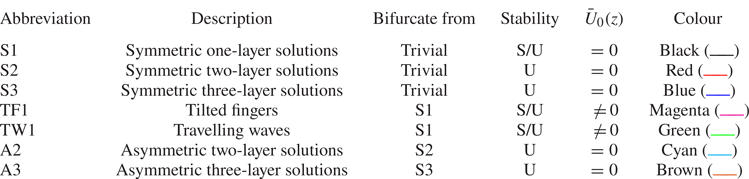
 $Ra_T=10^5$ for a direct comparison with DNS results (Yang et al. Reference Yang, van der Poel, Ostilla-Mónico, Sun, Verzicco, Grossmann and Lohse2015, Reference Yang, Verzicco and Lohse2016a). Table 2 provides a summary of the solutions, all of which are described in more detail in the following. All the solutions in the table are steady-state solutions, including the travelling waves (TW1) which are computed as steady states in a frame moving with the phase speed
 $c$ of the wave. This speed solves a nonlinear EVP. The bifurcation diagrams presented in this work (figures 2, 11, 14, 18 and 20) all show the time-averaged Sherwood number
 $Sh$ as a function of the horizontal domain size
 $L_x$ or equivalently the fundamental wavenumber
 $k_x=2{\rm \pi} /L_x$, where
 \begin{equation} Sh:=\langle \partial_z S |_{z=0} \rangle_{h,t}+1 \end{equation}
with  $\langle \,{\cdot }\, \rangle _{h,t}$ indicating average in both the horizontal direction and over time. Without confusion,
 $\langle \,{\cdot }\, \rangle _{h,t}$ is also referred to as a mean. In particular, for steady-state single-mode solutions, we obtain
 \begin{equation} Sh=\langle \partial_z \bar{S}_0 |_{z=0}\rangle_{t}+1=\partial_z\bar{S}_0|_{z=0}+1, \end{equation}
where  $\langle \,{\cdot }\, \rangle _t$ denotes time-averaging. We also use
 $\langle \,{\cdot }\, \rangle _h$ to denote averaging in the horizontal. For time-dependent solutions such as those obtained from DNS, these two types of averaging yield distinct results.
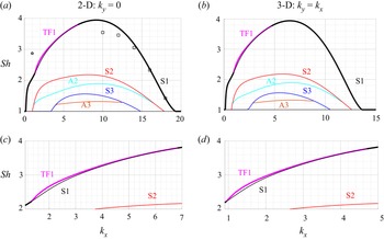
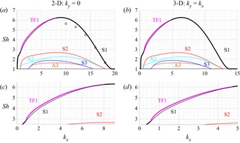
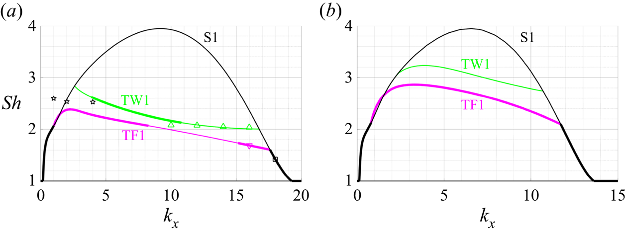
Bifurcation diagrams as a function of the fundamental wavenumber  $k_x$ from the single-mode equations (2.7) for (a) two dimensions,
 $k_y=0$, (b) three dimensions,
 $k_y=k_x$, and the parameters
 $R_\rho =40$,
 $Pr=7$,
 $\tau =0.01$ and
 $Ra_T=10^5$. The black squares show the
 $Sh$ of the steady state reached using 2-D DNS in domains of size
 $L_x=2{\rm \pi} /k_x$ (table 3); the black pentagram corresponds to DNS with
 $L_x=2{\rm \pi}$ displaying persistent chaotic behaviour. Panels (c) and (d) show enlarged views of the 2-D and 3-D results near the TF1 branch, respectively.

Summary of solution features, stability, induced large-scale shear  $\bar {U}_0(z)$ and line colour employed in the bifurcation diagrams (figures 2, 11, 14, 18 and 20). Symmetry is with respect to midplane reflection. Here S/U indicates both stable and unstable solutions exist along this solution branch and U indicates that only unstable solutions were found.

In the bifurcation diagrams reported in the following, we use thick lines to indicate stable solutions whereas thin lines represent unstable solutions. When the maximum amplitude of the large-scale shear mode  ${\text {max}}_{z}\,|\bar {U}_0(z)|$ along a branch is of the order of machine precision or smaller we report it as zero (table 2). In all other cases
 $\bar {U}_0(z)\neq 0$. When a large-scale shear is not generated,
 $\bar {U}_0=0$, the harmonic quantities
 $\hat {w}(z,t)$,
 $\tilde {u}(z,t):=-\text {i}\hat {u}(z,t)$,
 $\hat {S}(z,t)$ and
 $\hat {T}(z,t)$ are real for a suitably chosen phase. Here, the definition of
 $\tilde {u}(z,t)$ is motivated by the continuity equation
 $\text {i}k_x \hat {u}+\partial _z\hat {w}=0$ indicating that for a suitable choice of phase both
 $\tilde {u}(z,t)$ and
 $\hat {w}(z,t)$ may be simultaneously real-valued. This is the case whenever
 $\bar {U}_0=0$. However, for solutions associated with an induced large-scale shear (
 $\bar {U}_0\neq 0$) this is no longer so, and we denote the real and imaginary parts of the harmonic profile by
 ${\rm Re}[\,{\cdot }\,]$ and
 ${\rm Im}[\,{\cdot }\,]$, respectively. We refer to the base state in which all variables within the single-mode theory vanish as the trivial state. This state corresponds to
 $Sh=1$. Instabilities of this state generate the primary solution branches referred to as S1, S2 and S3. These branches are continued from their respective origin on the trivial branch, and their stability and secondary bifurcation points are examined. These give rise to the TF1, TW1, A2 and A3 solution branches which are also continued as detailed in table 2. Except for the results with stress-free velocity boundary conditions in § 3.2, all our results are computed for no-slip boundary conditions.
3.1. Solution profiles and comparison with DNS at $R_\rho =40$

We start from the dynamics near onset when  $R_\rho =40$, i.e. for
 $R_\rho \tau \sim O(1)$. This is the parameter regime close to the onset of the salt-finger instability, which occurs at
 $R_{\rho,{crit}}=1/\tau$ in vertically periodic domains (Radko Reference Radko2013, (2.4)) previously studied by Radko & Stern (Reference Radko and Stern1999, Reference Radko and Stern2000), Xie et al. (Reference Xie, Miquel, Julien and Knobloch2017) and Xie, Julien & Knobloch (Reference Xie, Julien and Knobloch2019). We focus on the bifurcation diagram as a function of
 $k_x$ measuring the finger width, and compare the results with DNS in domains of length
 $L_x=2{\rm \pi} /k_x$. This approach provides insight into the effects of the domain size on a system with a characteristic scale, here
 $d$, much as in Rayleigh–Bénard convection (van der Poel et al. Reference van der Poel, Stevens, Sugiyama and Lohse2012; Wagner & Shishkina Reference Wagner and Shishkina2013; Goluskin et al. Reference Goluskin, Johnston, Flierl and Spiegel2014).
Figure 2 shows the bifurcation diagram at  $R_\rho =40$ with no-slip boundary conditions. We consider both 2-D results with
 $k_y=0$ in figure 2(a) and 3-D results with
 $k_y=k_x$ in figure 2(b) indicating the same aspect ratio in the
 $x$ and
 $y$ horizontal directions. Here, the bifurcation diagram for the 3-D states with no large-scale flow
 $\bar {U}_0$ can be transformed into the diagram for the 2-D states upon defining an equivalent 2-D horizontal wavenumber
 \begin{equation} k_{x,2-D}=\sqrt{k_x^2+k_y^2}. \end{equation}
This is because the horizontal wavenumbers in the single-mode equations (2.7) for these states always appear in the combination  $k_x^2+k_y^2$. This is not the case when
 $\bar {U}_0\neq 0$ and in this case the TF1 states are indeed no longer identical as elaborated in figures 14 and 20.
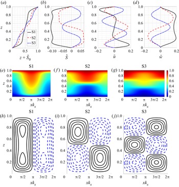
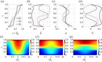
The solutions S1, S2 and S3 all bifurcate from the trivial solution. The S1, S2 and S3 solution profiles with  $k_x=8$,
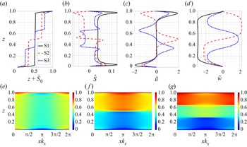
 $k_y=0$ are shown in figure 3. The horizontally averaged total salinity profiles
 $z+\bar {S}_0(z)$ in figure 3(a) show that these solutions are associated with one, two and three mixed layers, respectively, with reduced vertical gradient, resembling the staircase structures observed in field measurements (e.g. Schmitt et al. Reference Schmitt, Perkins, Boyd and Stalcup1987). Staircase-like solutions are also shown in some snapshots from 2-D DNS (Piacsek & Toomre Reference Piacsek and Toomre1980, figure 2) and reproduced by Zhang et al. (Reference Zhang, Wang, Lin, Zhu and Zeng2018, figure 3). Recent 3-D DNS results show the coexistence of multiple states with one, two or three mixed regions using different initial conditions (Yang et al. Reference Yang, Chen, Verzicco and Lohse2020, figure 2). In all three cases the mixed regions correspond to large values of the salinity amplitude
 $\hat {S}$ as shown in figure 3(b), as well as a large vertical velocity
 $\hat {w}$ as shown in figure 3(d). In contrast, the horizontal velocity in figure 3(c) peaks outside of the mixed region in each solution. See § 3.3 for further discussion.
Solution profiles from the single-mode equations (2.7) in the form of S1, S2 and S3 when  $k_x=8$,
 $k_y=0$,
 $R_\rho =40$,
 $Pr=7$,
 $\tau =0.01$ and
 $Ra_T=10^5$. The first row shows the profiles of (a)
 $z+\bar {S}_0$, (b)
 $\hat {S}$, (c)
 $\tilde {u}$ and (d)
 $\hat {w}$. The second row shows the reconstructed total salinity using (2.6a) and (2.1) for (e) S1, ( f) S2 and (g) S3 solutions. The third row shows isocontours of the streamfunction for (h) S1, (i) S2 and (j) S3 solutions.

The second row of figure 3 reconstructs the total salinity using (2.6a) and (2.1), whereas the third row of figure 3 shows the isocontours of the 2-D streamfunction computed as  $\psi (x,z)=\bar {\psi }_0(z)+\hat {\psi }(z){\rm e}^{\text {i}k_x x}+{\rm c.c.}$ with
 $\bar {\psi }_0(z)=-\int _0^z\bar {U}_0(\xi )\,{\rm d} \xi$ and
 $\hat {\psi }=\hat {w}/(\text {i}k_x)$. The isocontours are equispaced between
 $\pm$0.9 of the maximum value. The solid (black) line is used for positive (clockwise) streamlines whereas the dashed (blue) line indicates negative (counterclockwise) streamlines throughout this work. These results suggest that each mixed region is associated with one downward and one upward moving plume. As salinity tends to be homogenised in regions of closed steady streamlines (Rhines & Young Reference Rhines and Young1983) whereas salinity gradients are expelled from these regions, the resulting mean salinity exhibits an overall staircase-like profile.
Previous analysis of salt-finger convection in the spirit of single-mode solutions (Proctor & Holyer Reference Proctor and Holyer1986; Radko & Stern Reference Radko and Stern2000) also found the S1 type of solution, but S2 and S3 solutions were not found. This is likely because these studies (Proctor & Holyer Reference Proctor and Holyer1986; Radko & Stern Reference Radko and Stern2000) focused on the asymptotic behaviour close to the onset of instability but did not go beyond the first bifurcation point from the trivial solution.
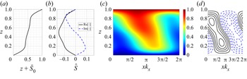
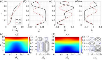
We also examined secondary bifurcations of the solutions S1, S2 and S3 in figure 2(a), focusing on the bifurcation points closest to their high wavenumber onset. The resulting secondary branches are of two types, corresponding to tilted fingers (TF1) and asymmetric layer spacing (A2 and A3). These states break the left–right reflection and the midplane reflection symmetry, respectively, as revealed by the corresponding solution profiles shown in figures 4 and 5. The mean salinity profile  $z+\bar {S}_0$ for TF1 in figure 4(a) is associated with two mixed regions near
 $z\in [0.2,0.4]$ and
 $z\in [0.6,0.8]$, whereas in the interior
 $z\in [0.4,0.6]$ the profile is close to linear. The corresponding profile of
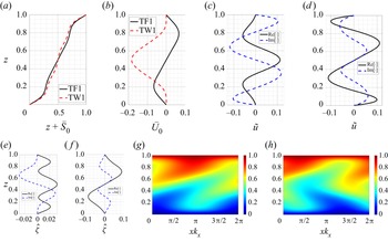
 $\hat {S}$ in figure 4(b) has both real and imaginary components with even and odd symmetry with respect to the midplane, respectively, indicating that the harmonics are no longer in phase in the vertical. The reconstructed total salinity shown in figure 4(c) reveals that the finger is now tilted; see also the streamfunction shown in figure 4(d). The tilted finger generates a non-zero large-scale shear with
 $\max _{{z}}\,\bar {U}_0(z)=3.16\times 10^{-4}$. The profile of the large-scale shear is shown farther below (figures 17a and 21b) for parameter values for which it is much stronger. A similar tilted finger state accompanied by large-scale shear was observed in earlier simulations of the single-mode equations (Paparella & Spiegel Reference Paparella and Spiegel1999) whereas observations of tilted fingers are reported in the NATRE (St. Laurent & Schmitt Reference St. Laurent and Schmitt1999, figure 3) and C-SALT field measurements (Kunze Reference Kunze1990, figure 1b) as well as in laboratory experiments on salt-finger convection; see, e.g. Taylor & Bucens (Reference Taylor and Bucens1989, figure 2) and Krishnamurti (Reference Krishnamurti2009, figure 2). Shear-associated tilting has also been widely reported in experiments on Rayleigh–Bénard convection (Krishnamurti & Howard Reference Krishnamurti and Howard1981) as well as in DNS of 2-D Rayleigh–Bénard convection (Goluskin et al. Reference Goluskin, Johnston, Flierl and Spiegel2014); see the review by Siggia (Reference Siggia1994).
Solution profiles of the TF1 state from the single-mode equations (2.7) with  $k_x=4$,
 $k_y=0$,
 $R_\rho =40$,
 $Pr=7$,
 $\tau =0.01$ and
 $Ra_T=10^5$. Panels (a) and (b) show the profiles of
 $z+\bar {S}_0$ and
 $\hat {S}$, respectively, whereas panels (c) and (d) show the reconstructed total salinity using (2.6a) and (2.1) and the isocontours of the streamfunction.

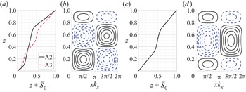
Solution profiles of the A2 and A3 states from the single-mode equations (2.7) with  $k_x=8$,
 $k_y=0$,
 $R_\rho =40$,
 $Pr=7$,
 $\tau =0.01$ and
 $Ra_T=10^5$. The first row shows the profiles of (a)
 $z+\bar {S}_0$, (b)
 $\hat {S}$, (c)
 $\tilde {u}$ and (d)
 $\hat {w}$. The second row shows the reconstructed total salinity using (2.6a) and (2.1) and the isocontours of the streamfunction for (e) A2 and ( f) A3.

The solution profiles in figures 5(a)–5(d) indicate that the A2 and A3 solutions spontaneously break the midplane reflection symmetry; states obtained via reflection in the midplane are therefore also solutions. In particular, the profile  $z+\bar {S}_0(z)$ no longer passes through
 $(1/2,1/2)$. However, the reconstructed total salinity profile and the isocontours of the streamfunction in figures 5(e) and 5( f) still resemble, qualitatively, the S2 and S3 profiles that distinguish these two asymmetric solutions. In particular, the A2 streamlines show two counter-rotating but unequal rolls in the vertical whereas the A3 solution exhibits three counter-rotating rolls, much as in the S2 and S3 states shown in figures 3(i) and 3(j). Solutions that are asymmetric with respect to midplane reflection have been seen in magnetoconvection with a depth-dependent magnetic diffusivity (Julien, Knobloch & Tobias Reference Julien, Knobloch and Tobias2000, figure 17) but are a consequence of forced symmetry breaking. Here, such asymmetric solutions originate from spontaneous symmetry breaking.
The stability of these solutions is indicated by thick (stable) and thin (unstable) lines in figure 2. The single-mode S1 solution is stable near both ends but loses stability to TF1 for intermediate wavenumbers  $k_x$. However, in either case the stable solution corresponds to the largest
 $Sh$ among all the solutions shown in the figure, a finding that is broadly consistent with the ‘relative stability’ criterion of Malkus & Veronis (Reference Malkus and Veronis1958). However, this is no longer so for smaller Prandtl numbers, as discussed in § 4.
The dynamics of unstable solutions are typically not easy to isolate and analyse without suitable initial conditions. Here, we use our single-mode solutions as initial conditions for 2-D DNS to provide additional insight into their stability. We set the horizontal domain size as  $L_x\in [2{\rm \pi} /18, 4{\rm \pi} ]$ and then use the single-mode solution profile at
 $k_x=2{\rm \pi} /L_x$,
 $k_y=0$, to construct a 2-D initial condition using the ansatz in (2.6). The final state after
 $t=3000$ for different
 $L_x$ and initial conditions based on S1, S2, S3 and TF1 solutions is summarised in table 3. For small horizontal domains (
 $L_x\leqslant 2{\rm \pi} /10$) the domain constrains the finger to be tall and thin and the DNS results with S1, S2 and S3 initial conditions all transition to a solution resembling the one-layer solution S1. This is consistent with the stability observation in the bifurcation diagram in figure 2. The DNS also provides the final
 $Sh$ numbers and these values are plotted using black squares in figure 2(a). The predicted
 $Sh$ from the single-mode solution is close to the DNS results, especially close to the high wavenumber onset of the S1 solution (
 $k_x=19.251$). The accuracy of the single-mode equations close to the high wavenumber onset is a consequence of the strong damping of modes with wavenumbers
 $k_x=2{\rm \pi} n/L_x$ (
 $n\in \mathbb {Z}$ and
 $n\geqslant 2$, e.g.
 $k_x=4{\rm \pi} /L_x$,
 $k_x=6{\rm \pi} /L_x$) that leaves only the trivial solution at these wavenumbers (see figure 2). As
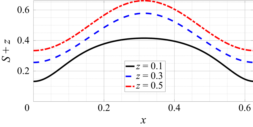
 $k_x$ decreases, the DNS results start to deviate from the single-mode predictions (figure 2a), a consequence of the departure of the horizontal salinity profile from the assumed sinusoidal form; see, e.g. the total salinity at
 $z=0.1$ in figure 6.
DNS results showing the total salinity  $z+S(x,z,t)$ across an S1 finger at
 $z=0.1$, 0.3 and 0.5 in a
 $L_x=2{\rm \pi} /10$ domain with parameters
 $R_\rho =40$,
 $Pr=7$,
 $\tau =0.01$ and
 $Ra_{T}=10^5$.

The flow structures from 2-D DNS simulations at  $t=3000$ in domains of size
 $L_x$ and initial condition (IC) constructed from S1, S2, S3 and TF1 solutions using the ansatz (2.6) with
 $k_x=2{\rm \pi} /L_x$,
 $k_y=0$. RTF indicates direction-reversing tilted fingers and C represents chaotic behaviour; ‘—’ indicates that a non-zero single-mode solution at
 $k_x=2{\rm \pi} /L_x$ is not present based on figure 2(a). The number
 $n\in \mathbb {Z}$ inside a bracket indicates that the final horizontal wavenumber reached by the solution is
 $k_x= 2{\rm \pi} n/L_x$,
 $n>1$, i.e. that the evolution results in a changed wavenumber.

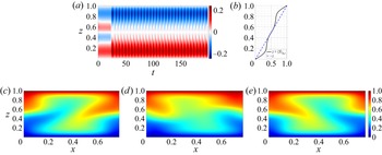
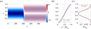
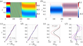
The final states in a domain of size  $L_x=2{\rm \pi} /8$ initialised by S2 and S3 show different flow structures. Figure 7 shows DNS results initialised with S2 and
 $L_x=2{\rm \pi} /8$. The horizontally averaged salinity deviation
 $\langle S\rangle _{h}(z,t)$ in figure 7(a) takes the requisite two-layer form for short times but then begins to oscillate in time. After averaging over time and in the horizontal direction, the total salinity profile
 $z+\langle S\rangle _{h,t}$ in figure 7(b) shows two mixed regions, with a broad interior region that is close to a linear profile. In fact, this oscillation and the two associated mixed regions in the mean salinity profile persist to at least
 $t=30{,}000$ (not shown). This behaviour is similar to the TF1 single-mode solution as shown in figure 4(a). The mean salinity profile in figure 7(b) also resembles the mean temperature profile in Rayleigh–Bénard convection with induced large-scale shear (Goluskin et al. Reference Goluskin, Johnston, Flierl and Spiegel2014, figure 5b), where the temperature profile shows two mixed regions close to the boundary, and an interior that approaches a linear profile with increasing Rayleigh number. The three snapshots of the total salinity in figures 7(c)–7(e) reveal that this behaviour is associated with a new state, a direction-reversing tilted finger (RTF). Such behaviour is also observed within simulations of the single-mode equations (Paparella & Spiegel Reference Paparella and Spiegel1999) (termed a layering instability there) and is accompanied by an oscillating large-scale shear. The direction-reversing tilted finger state also resembles (at least phenomenologically) the ‘pulsating wave’ found by Proctor et al. (Reference Proctor, Weiss, Brownjohn and Hurlburt1994, figure 7) and Matthews et al. (Reference Matthews, Proctor, Rucklidge and Weiss1993, figure 5) in magnetoconvection as well as large-scale flow reversals observed in Rayleigh–Bénard convection (Sugiyama et al. Reference Sugiyama, Ni, Stevens, Chan, Zhou, Xi, Sun, Grossmann, Xia and Lohse2010; Chandra & Verma Reference Chandra and Verma2013; Winchester, Dallas & Howell Reference Winchester, Dallas and Howell2021). We have not explored the origin of this state but note that similar ‘pulsating waves’ in other systems originate from a sequence of local and global bifurcations of a tilted convection roll (Matthews et al. Reference Matthews, Proctor, Rucklidge and Weiss1993; Proctor et al. Reference Proctor, Weiss, Brownjohn and Hurlburt1994; Rucklidge & Matthews Reference Rucklidge and Matthews1996).
Two dimensional DNS showing (a) horizontally averaged salinity  $\langle S\rangle _{h}(z,t)$ and (b) time-averaged and horizontally averaged total salinity
 $z+\langle S\rangle _{h,t}$. The second row shows isocontours of the total salinity
 $z+S(x,z,t)$ at (c)
 $t=32$, (d)
 $t=35$ and (e)
 $t=38$. The horizontal domain size is
 $L_x=2{\rm \pi} /8$ with initial condition in the form of a S2 single-mode solution with
 $k_x=2{\rm \pi} /L_x=8$,
 $k_y=0$. The parameters are
 $R_\rho =40$,
 $Pr=7$,
 $\tau =0.01$ and
 $Ra_{T}=10^5$. See supplementary movie 1 available at https://doi.org/10.1017/jfm.2022.865.

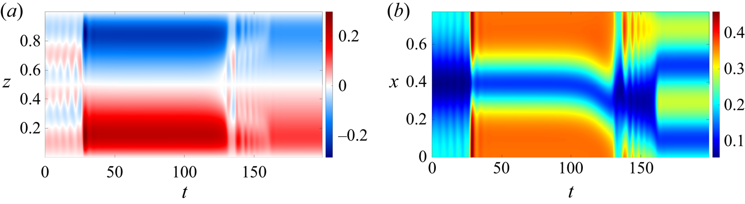
Figure 8 shows the DNS results with an S3 initial condition and  $L_x=2{\rm \pi} /8$ and displays the dynamics that are typically involved in transitioning to a higher wavenumber S1 solution. The profile of
 $\langle S\rangle _h$ in figure 8(a) initially shows a three-layer structure but starts to oscillate prior to a transition to the one-layer state S1 at
 $t\approx 30$. After
 $t\approx 160$, this one-layer solution transitions to another one-layer solution but with a smaller magnitude in
 $\langle S \rangle _{h}$. The total salinity near the lower boundary,
 $z=0.1$, is shown in figure 8(b) and further explains this transition scenario. The one-layer solution starts to tilt at
 $t\approx 110$ and begins to show oscillations at
 $t\approx 130$. Beyond
 $t\approx 160$, the horizontal wavenumber doubles leading to the S1 (2) state in table 3. Such a transition to a higher wavenumber S1 solution is also observed with horizontal domains
 $L_x\in [2{\rm \pi} /6, 2{\rm \pi} /2]$, albeit with different possibilities for the final wavenumber. Note that such transitions between different horizontal wavenumbers are not possible within the single-mode approach.
Two dimensional DNS results showing (a) the horizontally averaged salinity  $\langle S\rangle _h(z,t)$ and (b) the total salinity
 $z+S(x,z,t)$ at
 $z=0.1$. The horizontal domain size is based on
 $L_x=2{\rm \pi} /8$ with S3 single-mode initial condition with
 $k_x=2{\rm \pi} /L_x=8$ and
 $k_y=0$. The parameters are
 $R_\rho =40$,
 $Pr=7$,
 $\tau =0.01$ and
 $Ra_{T}=10^5$. See supplementary movie 2 available at https://doi.org/10.1017/jfm.2022.865.

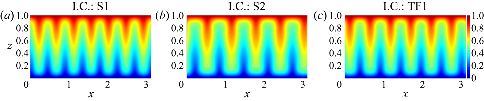
For  $L_x={\rm \pi}$, the final state shows different horizontal wavenumbers depending on the three different initial conditions S1, S2 and TF1 as indicated in table 3. The total salinity at
 $t=3000$ in these three final states is shown in figure 9. Although the horizontal domain size and the governing parameters are the same, different initial conditions lead to different final horizontal wavenumbers and the DNS results suggest that these persist up to at least
 $t=3000$. This observation suggests that for
 $L_x={\rm \pi}$ the three initial conditions S1, S2 and TF1 all lie in the basin of attraction of S1 solutions but associated with different and larger horizontal wavenumbers. This is, of course, a consequence of the preferred horizontal scale of the fingers. Note that the S3 solution does not exist for this domain size; see figure 2(a) and table 3. Rolls with different horizontal wavenumber obtained from different initial conditions are a familiar phenomenon in Rayleigh–Bénard convection (Wang et al. Reference Wang, Verzicco, Lohse and Shishkina2020) and in spanwise rotating plane Couette flow (Xia et al. Reference Xia, Shi, Cai, Wan and Chen2018; Yang & Xia Reference Yang and Xia2021).
Two dimensional DNS results for the total salinity  $z+S(x,z,t)$ at
 $t=3000$ in a horizontal domain of size
 $L_x={\rm \pi}$ initialised by (a) S1, (b) S2 and (c) TF1 single-mode solutions with
 $k_x=2{\rm \pi} /L_x=2$ and
 $k_y=0$.

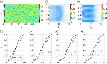
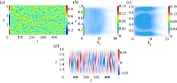
Solutions that do not reach a well-organised structure will be referred to as chaotic. Such behaviour is observed in large  $L_x$ domains. For example, single-mode S1 solutions with
 $k_x=1$ (
 $L_x=2{\rm \pi}$) and
 $k_x=0.5$ (
 $L_x=4{\rm \pi}$) are stable as shown in figure 2(a) but DNS initialised by these solutions ultimately exhibit chaotic behaviour. This is a consequence of the harmonics of the fundamental wavenumber
 $k_x$ included in the DNS. The total salinity in the midplane for
 $L_x=2{\rm \pi}$ is shown in figure 10(a), and displays chaotic behaviour with multiple downward and upward plumes in the horizontal. In order to further characterise the horizontal length scale, we computed
 $\langle |\mathcal {F}_x(S)|\rangle _t(z;k_x)$ and
 $\langle |\mathcal {F}_x(u)|\rangle _t(z;k_x)$, where
 $\mathcal {F}_x(\,{\cdot }\,)$ is the Fourier transform in the
 $x$-direction and
 $|\,{\cdot }\,|$ represents the modulus of the obtained complex Fourier coefficients. The results are shown in figures 10(b) and 10(c). The
 $k_x=0$ component of
 $\langle |\mathcal {F}_x(\,{\cdot }\,)|\rangle _t(z;k_x)$ is related to the amplitude of the horizontal mean
 $(\,\bar {\cdot }\,)_0$ whereas the
 $k_x\neq 0$ contributions to
 $\langle |\mathcal {F}_x(\,{\cdot }\,)|\rangle _t(z;k_x)$ are associated with the harmonic components
 $(\,\hat {\cdot }\, )$ in the single-mode ansatz (2.6). Figure 10(b) displays a peak at
 $k_x=0$ that corresponds to the deviation of the mean salinity from its linear profile. A second peak around
 $k_x\approx 9$ in figure 10(b) corresponds to a wavenumber that is close to that providing the largest
 $Sh$ in the S1 solution shown in figure 2(a). However, in the midplane, the peak wavenumber shifts to
 $k_x= 13$.
Two dimensional DNS results displaying (a) total salinity  $z+S(x,z,t)$ at
 $z=1/2$, (b)
 $\langle |\mathcal {F}_x(S)| \rangle _t(z;k_x)$, (c)
 $\langle |\mathcal {F}_x(u)| \rangle _t(z;k_x)$, (d)
 $z+\langle S\rangle _{h,t}(z)$, and snapshots of the horizontally averaged total salinity
 $z+\langle S\rangle _h(z,t)$ at (e)
 $t=416$, ( f)
 $t=437$ and (g)
 $t=478$. The horizontal domain size is
 $L_x=2{\rm \pi}$ initialised by a S1 solution with
 $k_x=2{\rm \pi} /L_x=1$,
 $k_y=0$. The governing parameters are
 $R_\rho =40$,
 $Pr=7$,
 $\tau =0.01$ and
 $Ra_T=10^5$.

The Fourier transform of the horizontal velocity enables us to isolate the role of the S1, S2 and S3 solutions. The plot of  $\langle |\mathcal {F}_x(u)| \rangle _t(z;k_x)$ in figure 10(c) reveals a stronger peak at
 $k_x=9$ but now at multiple locations dominated by regions near the boundaries, with a lower amplitude near
 $z=1/3$ and
 $2/3$, the peak region of the horizontal velocity
 $\tilde {u}$ in the three-layer solution S3 shown in figure 3(c). Note that the horizontal velocity in the S1 and S2 solutions almost vanishes at these locations as shown in figure 3(c). Furthermore,
 $\langle |\mathcal {F}_x(u)| \rangle _t(z;k_x)$ also shows a local peak at
 $k_x=1$ near the midplane resembling the horizontal velocity
 $\tilde {u}$ of the two-layer solution S2, whereas the horizontal velocity in the S1 and S3 single-mode solutions vanishes in the midplane as shown in figure 3(c). These observations suggest that the unstable S2 and S3 solutions both play a role in the chaotic behaviour and that their properties may manifest themselves in the statistics of the chaotic state, cf. Kawahara & Kida (Reference Kawahara and Kida2001) and the reviews by Kawahara et al. (Reference Kawahara, Uhlmann and van Veen2012) and Graham & Floryan (Reference Graham and Floryan2021).
In order to further quantify the role of unstable solutions, we plot in figures 10(e)–10(g) the horizontally averaged profiles at three different times for comparison with the horizontally averaged time-averaged state in figure 10(d). Although the salinity profile in the latter state does not show a significant staircase, the horizontally averaged salinity profiles at the two times shown in figures 10(e) and 10( f) do in fact show a tendency towards three and two steps, respectively, whereas the snapshot in figure 10(g) shows instead a salinity profile that temporarily breaks the midplane reflection symmetry. These results provide evidence that the chaotic state visits the neighbourhood of not only the unstable staircase-like solutions S2 and S3 but also of the asymmetric solution. The time-averaged  $Sh$ within
 $t\in [100,500]$ is
 $Sh\approx 2.8693$, a value lower than the maximum
 $Sh$ for S1 but higher than those for S2 and S3 at the suggested peak wavenumber
 $k_x=9$ as shown in figure 2(a), and suggests that these states may play a role in determining the time-averaged salinity transport in this chaotic state.
3.2. No-slip versus stress-free boundary conditions
Although no-slip boundary conditions are relevant for experiments (Hage & Tilgner Reference Hage and Tilgner2010), stress-free boundary conditions are more appropriate for oceanographic applications. Here we compare the bifurcation diagram in the no-slip case with the corresponding diagram with stress-free boundary conditions. For this purpose we replace the original no-slip boundary conditions in (2.5) by the stress-free boundary conditions
 $$\begin{gather} w(x,y,z=0,t)=w(x,y,z=1,t)=0, \end{gather}$$
 $$\begin{gather}\partial_z u(x,y,z=0,t)=\partial_z u(x,y,z=1,t)=0, \end{gather}$$
 $$\begin{gather}\partial_z v(x,y,z=0,t)=\partial_z v(x,y,z=1,t)=0. \end{gather}$$
Within the single-mode equations, the corresponding velocity boundary conditions in (2.9) are thus replaced as
 $$\begin{gather} \hat{w}(z=0,t)=\hat{w}(z=1,t)=\partial_{z}^2\hat{w}(z=0,t)=\partial_{z}^2\hat{w}(z=1,t) \end{gather}$$
 $$\begin{gather}=\partial_z\hat{\zeta}(z=0,t)=\partial_z\hat{\zeta}(z=1,t)=\partial_z\bar{U}_0(z=0,t)=\partial_z\bar{U}_0(z=1,t)=0. \end{gather}$$
Note that the governing equations with stress-free boundary conditions admit an additional Galilean symmetry: the large-scale shear can be shifted by an arbitrary constant,  $\bar {U}_0\rightarrow \bar {U}_0+C$. To obtain unique solutions we therefore impose the additional constraint
 $\int _{0}^{1}\bar {U}_0(z,t)\,{\rm d} z=0$ following the procedure in Uecker (Reference Uecker2021a, § 6.9).
Figure 11 shows the resulting bifurcation diagrams for comparison with figure 2. The diagrams are very similar: all of the previously discussed solution branches are still present. The main difference is that the stress-free boundary conditions typically lead to a larger  $Sh$ than the no-slip boundary conditions at the same horizontal wavenumber. This behaviour is also consistent with the observation by Yang, Verzicco & Lohse (Reference Yang, Verzicco and Lohse2016b), where 3-D DNS results indicate that the flow morphology is qualitatively similar but stress-free boundary conditions display a larger
 $Sh$. Figure 11(a) compares the single-mode results with the corresponding steady state
 $Sh$ reached using 2-D DNS in domains of size
 $L_x=2{\rm \pi} /k_x$ (black squares) showing good agreement provided the domain width
 $L_x$ is sufficiently narrow, i.e. for
 $k_x$ sufficiently close to the stress-free onset wavenumber
 $k_x=19.298$.
Bifurcation diagrams computed from the single-mode equations (2.7) with the same parameter values as in figure 2 but stress-free velocity boundary conditions at the top and bottom. The black squares show the corresponding steady state  $Sh$ reached using 2-D DNS in domains of size
 $L_x=2{\rm \pi} /k_x$. Panels (c) and (d) show enlarged views of the 2-D and 3-D results near the TF1 branch, respectively.

Figure 12 displays solution profiles and total salinity for the S1, S2 and S3 solutions at the same parameter values as in figure 3 but with stress-free instead of no-slip boundary conditions. Here, the horizontally averaged total salinity  $z+\bar {S}_0$ still displays the one-layer, two-layer and three-layer solution profiles in the vertical. The horizontal structure of these states is qualitatively similar to the no-slip results in figure 3. The main difference is that the horizontal velocity
 $\tilde {u}$ and the gradient of vertical velocity
 $\partial _z \hat {w}$ no longer vanish at the boundaries.
Solution profiles from the single-mode equations (2.7) in the same parameter regime as figure 3 but with stress-free velocity boundary conditions at the top and bottom. The first row shows the profiles of (a)  $z+\bar {S}_0$, (b)
 $\hat {S}$, (c)
 $\tilde {u}$ and (d)
 $\hat {w}$. The second row shows the reconstructed total salinity using (2.6a) and (2.1) for (e) S1, ( f) S2 and (g) S3 solutions.

Figure 13(a) displays the A2 and A3 solution profiles with stress-free boundary conditions. The A2 solution exhibits a similar profile as in the no-slip boundary condition case shown in figure 5(a), whereas the horizontally averaged salinity in A3 differs from that found with the no-slip boundary conditions. Figure 13(b) shows the isocontours of the streamfunction in A3, and shows two large and one small recirculation cell in the vertical direction, whereas figure 5( f) shows one large and two small cells in the vertical. Here, the A3 solution in the stress-free boundary condition case originates from a secondary bifurcation at  $k_x=13.665$ on the S3 branch, whereas there is another secondary bifurcation at
 $k_x=13.703$ (not shown in figure 11) that is closer to the high wavenumber onset of the S3 state
 $(k_x=15.573)$ and that preserves midplane reflection symmetry. The mean salinity of the state shown in figure 13(c) resembles the mean temperature profile in magnetoconvection (Julien et al. Reference Julien, Knobloch and Tobias2000, figure 7b), and the isocontours of the streamfunction in figure 13(d) show one large and two small closed streamlines that are similar to those in the A3 solution with no-slip boundary conditions in figure 5( f). The fact that this additional secondary bifurcation appears closer to the high wavenumber onset of S3 than the bifurcation to the A3 branch likely contributes to the difference in the solution profiles of the A3 state with stress-free and no-slip boundary conditions.
Solution profiles on the secondary branches computed from the single-mode equations (2.7) in the same parameter regime as figure 5 but with stress-free velocity boundary conditions at the top and bottom. Panel (a) shows the profiles of  $z+\bar {S}_0$ of the A2 and A3 solutions, whereas panel (b) displays the isocontours of the streamfunction of the A3 solution. Panels (c) and (d) show
 $z+\bar {S}_0$ and the isocontours of the streamfunction for a steady solution preserving midplane reflection symmetry generated in a secondary bifurcation of the S3 solution.

3.3. Dependence on density ratio
Oceanographic conditions display a wide range of density ratios, and this subsection therefore explores the dependence of our results on the density ratio. In particular, the staircases observed in oceanographic observations, laboratory measurements and DNS are typically associated with the parameter regime  $R_\rho \sim O(1)$ (Schmitt et al. Reference Schmitt, Perkins, Boyd and Stalcup1987; Krishnamurti Reference Krishnamurti2003, Reference Krishnamurti2009; Radko Reference Radko2003) that is far away from the onset of the salt-finger instability
 $R_{\rho,{crit}}=1/\tau$ with
 $\tau =0.01$.
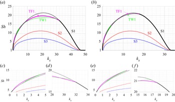
Figure 14 shows the bifurcation diagram with density ratio  $R_\rho =2$ and no-slip boundary conditions for (a) 2-D results with
 $k_y=0$ and (b) 3-D results with
 $k_y=k_x$. Here, we focus on the S1, S2, S3 and TF1 solution branches, as well as a new travelling wave (TW1) solution branch that does not exist when
 $R_\rho =40$. Note that in this case non-trivial solutions exist over a wider range of horizontal wavenumbers than for
 $R_\rho =40$ (figure 2), suggesting that the finger width depends not only on
 $Ra_T$ but also on the density ratio
 $R_\rho$. Here, the
 $Sh$ of the S1, S2 and S3 solutions in the 2-D and 3-D configurations are still the same after converting the results by rescaling the horizontal wavenumber according to (3.3). However, the stability of the S1 solutions is now different and the secondary bifurcation points on S1 that lead to TF1 and TW1 also differ. This can be seen in the enlarged views of regions close to the appearance of TF1 and TW1 in figures 14(c)–14( f). Specifically, the bifurcation points leading to the TF1 and TW1 branches in two dimensions are closer to the high wavenumber onset
 $k_x=46.884$ of the S1 solution than in three dimensions, suggesting that the 2-D configuration forms tilted fingers or travelling wave solutions more readily. This is consistent with the suggestion that large-scale shear is generated more easily in a 2-D configuration than in a 3-D configuration (Goluskin et al. Reference Goluskin, Johnston, Flierl and Spiegel2014).
Bifurcation diagrams as a function of the wavenumber  $k_x$ from the single-mode equations (2.7) with (a) two dimensions,
 $k_y=0$ and (b) three dimensions,
 $k_y=k_x$. The governing parameters are
 $R_\rho =2$,
 $Pr=7$,
 $\tau =0.01$, and
 $Ra_T=10^5$. Panels (c–d) are enlarged views of the 2-D results in panel (a) and panels (e–f) are enlarged views of the 3-D results in panel (b).

The S1, S2 and S3 solution branches at  $R_\rho =2$ in figure 14 exhibit much larger
 $Sh$ than those at
 $R_\rho =40$ in figure 2. This is expected as a lower density ratio indicates stronger destabilisation by the salinity gradient. Figure 15 shows profiles of the S1, S2 and S3 solutions at
 $R_\rho =2$ and
 $k_x=17.5$,
 $k_y=0$. Here, the mixed region in the horizontally averaged total salinity
 $z+\bar {S}_0(z)$ in figure 15(a) corresponds to almost constant salinity compared with the solution profile at
 $R_\rho =40$ in figure 3(a). Outside of this region, both the profile
 $z+\bar {S}_0(z)$ and the isocontours of total salinity in figures 15(e)–15(g) exhibit sharper interfaces than those at
 $R_\rho =40$ in figure 3. This is consistent with the observation of well-defined staircases in flow regimes with
 $R_\rho \sim O(1)$ in field measurements (Schmitt et al. Reference Schmitt, Perkins, Boyd and Stalcup1987) and laboratory experiments (Krishnamurti Reference Krishnamurti2003, Reference Krishnamurti2009) as well as in DNS (Radko Reference Radko2003). The vertical profiles of the salinity harmonic
 $\hat {S}$ in the S1, S2 and S3 states shown in figure 15(b) all show a local overshoot associated with the sharp interfaces. Both the horizontal velocity and the vertical velocity in figures 15(c)–15(d) show a larger magnitude compared with the
 $R_\rho =40$ results in figures 3(c)–3(d).
Solution profiles from the single-mode equations (2.7). The first row shows the profiles of (a)  $z+\bar {S}_0$, (b)
 $\hat {S}$, (c)
 $\tilde {u}$ and (d)
 $\hat {w}$. The second row shows the reconstructed total salinity using (2.6a) and (2.1) for (e) S1, ( f) S2 and (g) S3 solutions. The parameter values are
 $k_x=17.5$,
 $k_y=0$,
 $R_\rho =2$,
 $Pr=7$,
 $\tau =0.01$ and
 $Ra_T=10^5$.

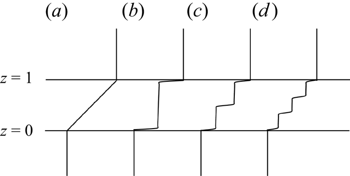
Figure 16 combines the mean salinity profiles of the S1, S2 and S3 single-mode solutions in figure 15(a) with constant salinity outside of the region  $z\in [0,1]$ on the assumption that each layer is well mixed. The figure shows that salt-finger convection can distort a linear mean salinity profile into a staircase-like profile in
 $z\in [0,1]$, particularly when
 $R_{\rho }$ is relatively small. Although other mechanisms may be involved in the ocean leading to layer formation, merger and migration, including the presence of a diffusive regime (cold fresh water on top of warm salty water) (Timmermans et al. Reference Timmermans, Toole, Krishfield and Winsor2008; Radko Reference Radko2016; Yang et al. Reference Yang, Verzicco, Lohse and Caulfield2022) or stratified shear flow (Oglethorpe, Caulfield & Woods Reference Oglethorpe, Caulfield and Woods2013; Lucas, Caulfield & Kerswell Reference Lucas, Caulfield and Kerswell2017; Taylor & Zhou Reference Taylor and Zhou2017; Lucas, Caulfield & Kerswell Reference Lucas, Caulfield and Kerswell2019), our work suggests that in horizontally extended domains shearing instabilities may disrupt the finger zones that form the S1, S2 and S3 profiles without destroying the associated staircase structure, leading to well-mixed layers of the type observed in the oceans.
Sketch of the mean total salinity profile  $z+\bar {S}_0(z)$ between two well-mixed regions, where the interior
 $z\in [0,1]$ is associated with (a) a linear base state, (b) S1 solution, (c) S2 solution and (d) S3 solution. The S1, S2 and S3 single-mode solutions are obtained from figure 15(a) associated with
 $k_x=17.5$,
 $k_y=0$,
 $R_\rho =2$,
 $Pr=7$,
 $\tau =0.01$ and
 $Ra_T=10^5$.

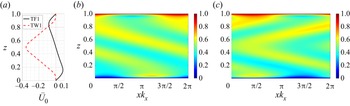
We now focus on the solutions TF1 and TW1 originating from secondary bifurcations of the S1 state. Figure 17(a) shows the associated large-scale shear  $\bar {U}_0(z)$ of TF1 and TW1. This shear is antisymmetric with respect to the midplane for TF1 but symmetric for TW1. Figure 17(b) shows the total salinity profile for a tilted finger with a larger tilt angle compared with the tilt at
 $R_\rho =40$ shown in figure 4(c). Figure 17(c) shows the total salinity of TW1 in the comoving frame, with structures that tilt in opposite directions above and below the midplane. This alternating tilt direction resembles the ‘wavy fingers’ tilted either left or right observed in experiments (Krishnamurti Reference Krishnamurti2003, figure 7), although whether such ‘wavy fingers’ travel depends on the boundary conditions in the horizontal.
Solution profiles from the single-mode equations (2.7) showing (a) the large-scale shear  $\bar {U}_0$ and the total salinity for (b) TF1 and (c) TW1. The governing parameters are
 $k_x=17.5$,
 $k_y=0$,
 $R_\rho =2$,
 $Pr=7$,
 $\tau =0.01$ and
 $Ra_T=10^5$.

The stability properties of these solutions are also indicated in figure 14 and are similar to those for high density ratios (figure 2). Here, the S1 solution is stable near the onset, but loses stability to tilted fingers. The solutions S2 and S3 are still unstable within all of the current parameter regime. The travelling wave appears to gain stability within a certain wavenumber regime close to the low wavenumber onset, as indicated in the enlarged views in figures 14(c) and 14(e). As the single-mode solutions are expected to be more accurate in the high wavenumber regime, cf. figure 2(a), we postpone a study of the dynamics of TF1 and TW1 to the lower Prandtl number considered in § 4 where these states form at higher wavenumbers.
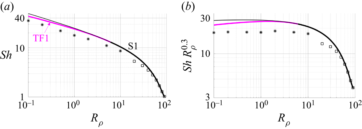
Figure 18 displays the dependence of the  $Sh$ on the density ratio
 $R_\rho$ for
 $\tau =0.01$ for 3-D results with
 $k_y=k_x$ based on the scaling law
 $$\begin{gather} k_x=k_y=R_\rho^{0.125}{\rm \pi}/(14.8211Ra_S^{{-}0.2428}), \end{gather}$$
 $$\begin{gather}Ra_S:=\frac{ g \beta\Delta S h^3}{\kappa_S\nu }=\frac{Ra_T}{R_\rho \tau}, \end{gather}$$
obtained through a least-squares fit of the finger width computed from 3-D DNS (Yang et al. Reference Yang, Verzicco and Lohse2016a, figure 13b). Here, we can see that the S1 solution remains stable near onset, and then bifurcates to stable tilted fingers (TF1) as  $R_\rho$ decreases. The figure also shows the
 $Sh$ from 3-D DNS data (Yang et al. Reference Yang, van der Poel, Ostilla-Mónico, Sun, Verzicco, Grossmann and Lohse2015, table 1) using black stars. We also perform 2-D DNS in domains of size
 $L_x=2{\rm \pi} /k_{x,2-D}=2{\rm \pi} /(\sqrt {2}k_x)$ with
 $k_x$ given by (3.6a). Note that our simulation results do not display a smooth transition to the
 $Sh$ from the 3-D results (Yang et al. Reference Yang, van der Poel, Ostilla-Mónico, Sun, Verzicco, Grossmann and Lohse2015), which is likely due to the intrinsic difference between 2-D and 3-D simulations and possibly different domain sizes. However, the
 $Sh$ obtained from the S1 single-mode solutions agree well with the DNS results near the high density ratio onset. At lower density ratios, the single-mode solution S1 and TF1 both overpredict the DNS results. This may be because both are steady-state solutions, whereas the DNS results exhibit time-dependent behaviour which likely reduces the time-averaged
 $Sh$ number.
(a) Bifurcation diagrams displaying  $Sh$ as a function of the density ratio
 $R_\rho$ from the single-mode equations (2.7) with wavenumbers
 $k_x$ and
 $k_y$ given by the scaling law (3.6a). The other parameters are
 $Pr=7$,
 $\tau =0.01$ and
 $Ra_T=10^5$. The black star
 $(*)$ is obtained from 3-D DNS (Yang et al. Reference Yang, van der Poel, Ostilla-Mónico, Sun, Verzicco, Grossmann and Lohse2015, table 1). The black square
 $(\square )$ is obtained from 2-D DNS results in a horizontal domain of size
 $L_x=2{\rm \pi} /k_{x,2-D}=2{\rm \pi} /(\sqrt {2}k_x)$ with
 $k_x$ given by (3.6a). (b) Plot of the results in (a) in compensated form to exhibit the scaling exponent.

We find that  $Sh\sim R_\rho ^{-0.30}$ for the single-mode solutions within the range
 $R_\rho \in [0.1,2]$ and fixed
 $Ra_T=10^5$ and
 $\tau =0.01$, indicating that for these values of
 $Ra_T$ and
 $\tau$,
 $Sh\sim Ra_S^{0.30}$ as a function of the salinity Rayleigh number defined in (3.6b). This result agrees well with the scaling law of the Nusselt number,
 $Nu\sim Ra_T^{0.30}(\ln Ra_T)^{0.20}$, obtained from single-mode solutions for Rayleigh–Bénard convection and wavenumber scaling as
 $k_x\sim Ra_T^{1/4}$ (Gough et al. Reference Gough, Spiegel and Toomre1975, p. 713). The scaling law in (3.6a) employed here with a fixed
 $R_\rho$ is also compatible with
 $k_x\sim Ra_T^{1/4}$ employed in Rayleigh–Bénard convection (Gough et al. Reference Gough, Spiegel and Toomre1975). Figure 18(b) displays the compensated Sherwood number
 $Sh\,R_\rho ^{0.30}$, showing that the S1 solutions from both the single-mode approach and DNS (Yang et al. Reference Yang, van der Poel, Ostilla-Mónico, Sun, Verzicco, Grossmann and Lohse2015) follow the same
 $Sh\sim R_\rho ^{-0.3}$ scaling law. Note that the DNS results for salt-finger convection in the asymptotic regime of high
 $Ra_S$ instead suggest
 $Sh\sim Ra_S^{1/3}$ (Yang et al. Reference Yang, van der Poel, Ostilla-Mónico, Sun, Verzicco, Grossmann and Lohse2015, figure 7a) whereas experimental results suggest
 $Sh\sim Ra_S^{4/9}$ (Hage & Tilgner Reference Hage and Tilgner2010, figure 8). The parameter regime considered here is within the regime
 $Ra_S\leqslant 10^8$, a value that may be insufficient to reliably establish the asymptotic scaling; see, e.g. Yang et al. (Reference Yang, van der Poel, Ostilla-Mónico, Sun, Verzicco, Grossmann and Lohse2015, figure 7a) and Yang et al. (Reference Yang, Verzicco and Lohse2016b, figure 3a). The TF1 solutions suggest the scaling law
 $Sh\sim R_\rho ^{-0.27}$ or
 $Sh\sim Ra_S^{0.27}$ for fixed
 $Ra_T$ and
 $\tau$. This is consistent with the observation in Rayleigh–Bénard convection that the formation of the large-scale shear decreases the scaling exponent
 $\eta$ of
 $Nu\sim Ra_T^{\eta }$; see, e.g. Goluskin et al. (Reference Goluskin, Johnston, Flierl and Spiegel2014, figure 4).
Figure 19 shows the corresponding mean salinity and temperature profiles at the same parameter values as those used for the 3-D DNS results in Yang et al. (Reference Yang, van der Poel, Ostilla-Mónico, Sun, Verzicco, Grossmann and Lohse2015, figure 2a). The solution profiles from the single-mode equations closely match the qualitative trend of the mean salinity and temperature profiles as a function of the density ratio in the DNS results (Yang et al. Reference Yang, van der Poel, Ostilla-Mónico, Sun, Verzicco, Grossmann and Lohse2015, figure 2a). In particular, both the single-mode and DNS results show that the mean salinity profile displays a mixed region in the layer interior, and that both show a small overshoot (a thin stably stratified region) near the top and bottom boundaries. The mean total temperature remains close to a linear profile, however, and shows a visible deviation from a linear profile only at  $R_\rho =0.1$, a fact also consistent with DNS observation (Yang et al. Reference Yang, van der Poel, Ostilla-Mónico, Sun, Verzicco, Grossmann and Lohse2015, figure 2a).
Solution profiles from the single-mode equations (2.7) displaying horizontally averaged total salinity (black solid lines) and horizontally averaged total temperature (blue dashed lines). Solution profiles are labeled by integers and correspond to  $R_\rho =10,5,2,1,0.5,0.2$ and
 $0.1$ from left to right. Other parameter values are
 $Pr=7$,
 $\tau =0.01$ and
 $Ra_T=10^5$, with
 $k_x=k_y$ given by the scaling law in (3.6a).

4. Tilted salt fingers and travelling waves at $Pr=0.05$

The bifurcation diagram for a low density ratio,  $R_\rho =2$, and
 $Pr=7$ displays a branch of steady tilted fingers (TF1) and a branch of travelling waves (TW1), both of which bifurcate from the symmetric one-layer solution S1 at intermediate wavenumbers. Here, we study these states in the low Prandtl number regime that pushes the bifurcations to TF1 and TW1 to higher wavenumbers and, hence, closer to the high wavenumber onset, where we expect the single-mode solutions to be accurate. Low Prandtl number salt-finger convection is of interest in astrophysical applications, where molecular weight gradients compete with thermal buoyancy but heat transport is dominated by photon diffusion (Garaud Reference Garaud2018). However, to keep the notation consistent with the previous sections, we continue to use the symbol
 $S$ to represent the higher molecular weight component and refer to it as salinity. The results presented here for
 $Pr=0.05$ parallel those for
 $Pr=7$ in § 3.1 in order to highlight the effect of a low Prandtl number.
Figure 20 shows the bifurcation diagram for the parameter values used in figure 2 but with  $Pr=0.05$. Here, we focus on the solution branches S1, TF1 and TW1; the S2 and S3 branches are omitted because neither their Sherwood number nor their overall stability changes when the Prandtl number changes from
 $Pr=7$ to
 $Pr=0.05$. Compared with the
 $Pr=7$ results in figure 2, we see that the
 $Sh$ associated with the S1 solution remains the same, but the bifurcation to TF1 (
 $k_x= 17.593$) now occurs much closer to the high wavenumber onset of the S1 solution (
 $k_x=19.251$). Moreover, the travelling wave branch TW1 that is present here does not appear at
 $R_\rho =40$,
 $Pr=7$ in figure 2. Evidently low Prandtl numbers favour spontaneous formation of large-scale shear, as found in DNS by Radko (Reference Radko2010, figures 1–2) and Garaud & Brummell (Reference Garaud and Brummell2015) as well as in a reduced model valid in the asymptotic limit of low
 $\tau$ and low
 $Pr$ (Xie et al. Reference Xie, Julien and Knobloch2019). A related phenomenon is found in Rayleigh–Bénard convection, where at low
 $Pr$ a steady convection roll becomes immediately unstable to a large-scale (zonal) mode (Winchester, Howell & Dallas Reference Winchester, Howell and Dallas2022).
Bifurcation diagrams as a function of the wavenumber  $k_x$ from the single-mode equations (2.7) in (a) two dimensions,
 $k_y=0$ and (b) three dimensions,
 $k_y=k_x$. Other parameters are
 $R_\rho =40$,
 $Pr=0.05$,
 $\tau =0.01$ and
 $Ra_T=10^5$. The markers correspond to the
 $Sh$ associated with steady states resembling S1 (
 $\square$), TF1 (
 $\triangledown$, magenta) and TW1 (
 $\triangle$, green) solutions from 2-D DNS in domains of size
 $L_x=2{\rm \pi} /k_x$ (table 4). The black pentagrams corresponding to the
 $Sh$ at
 $L_x=2{\rm \pi} /k_x$ (
 $k_x=1$, 2, 4) indicate chaotic behaviour.

A comparison between 2-D and 3-D results at  $Pr=0.05$ in figure 20 shows that the bifurcation point of TF1 and TW1 is closer to the high wavenumber onset of S1 in the 2-D configuration. The difference between the 2-D and 3-D configurations at
 $Pr=0.05$ in figure 20 is more evident than that at
 $Pr=7$ in figure 2, as is the case in Rayleigh–Bénard convection (van der Poel, Stevens & Lohse Reference van der Poel, Stevens and Lohse2013). Recalling that both TF1 and TW1 are associated with the formation of large-scale shear (see table 2, and figures 17a and 21b), this difference suggests that the 2-D configuration favours the formation of large-scale shear (cf. Garaud & Brummell Reference Garaud and Brummell2015).
Solution profiles from the single-mode equations (2.7) for the TF1 and TW1 solutions displaying (a)  $z+\bar {S}_0$, (b)
 $\bar {U}_0$ and the horizontal velocity
 $\tilde {u}$ for (c) TF1 and (d) TW1. The second row shows the vertical vorticity mode for (e) TF1 and ( f) TW1 and the total salinity for (g) TF1 and (h) TW1 using (2.6a) and (2.1). Other parameter values are
 $k_x=k_y=6.873$,
 $R_\rho =40$,
 $Pr=0.05$,
 $\tau =0.01$ and
 $Ra_T=10^5$.

Figure 21 shows the solution profiles in the TF1 and TW1 states. Here we choose a 3-D wavenumber  $k_y=k_x=6.873$ close to the wavenumber that maximises the
 $Sh$ in the S1 solution. Similar to the earlier observation of tilted fingers in figure 4, the mean total salinity profile
 $z+\bar {S}_0(z)$ of TF1 shows two mixed regions with a linear profile in the middle of the layer. In contrast, the TW1 shows instead a three-layer structure in
 $z+\bar {S}_0(z)$. Figure 21(b) displays the associated large-scale shear
 $\bar {U}_0(z)$, and exhibits a similar structure to that observed at
 $R_\rho =2$,
 $Pr=7$ in figure 17(a). Figures 21(c) and 21(d) display the vertical profile of the first harmonic of the horizontal velocity
 $\tilde {u}$ in the TF1 and TW1 states showing local peaks close to
 $z=1/3$,
 $1/2$ and
 $2/3$, in contrast to the corresponding S1 solution that displays peaks near the boundaries. These properties are, in turn, reflected in the staircase profile of the mean salinity shown in figure 21(a).
Furthermore, in three dimensions the TF1 and TW1 solutions are also associated with non-zero vertical vorticity as shown in figures 21(e) and 21( f). Here, the generation of the vertical vorticity originates from the large-scale horizontal shear  $\bar {U}_0$, which provides a source term for the vertical vorticity equation (2.7b). Vertical vorticity is also generated in bifurcations of steady convection rolls (resembling S1) in single-mode solutions of Rayleigh–Bénard convection on a hexagonal lattice (Lopez & Murphy Reference Lopez and Murphy1983; Murphy & Lopez Reference Murphy and Lopez1984; Massaguer & Mercader Reference Massaguer and Mercader1988; Massaguer et al. Reference Massaguer, Mercader and Net1990) with a source term provided by self-interaction on this lattice (e.g. Massaguer et al. Reference Massaguer, Mercader and Net1990, (2.2b)). As the current single-mode formulation is limited to roll or square planforms, this source term is not present. Instead, it is the associated large-scale shear
 $\bar {U}_0$ that provides the source term for vertical vorticity, a possibility not included in the previous work (Lopez & Murphy Reference Lopez and Murphy1983; Murphy & Lopez Reference Murphy and Lopez1984; Massaguer & Mercader Reference Massaguer and Mercader1988; Massaguer et al. Reference Massaguer, Mercader and Net1990).
The isocontours of total salinity of TF1 and TW1 are shown in figures 21(g) and 21(h). These panels show qualitative similarity with the TF1 and TW1 shown in figures 17(b) and 17(c), where the TF1 solution is tilted in one direction, whereas the TW1 is tilted in opposite directions above and below the midplane. However, the TF1 and TW1 at  $R_\rho =2$,
 $Pr=7$ in figure 17 show a relatively well-mixed region in the interior,
 $z\approx 1/2$, compared with the TF1 and TW1 at the higher density ratio
 $R_\rho =40$ but small Prandtl number,
 $Pr=0.05$, shown in figure 21.
The stability of these solutions is indicated in figure 20 by thick (stable) and thin (unstable) lines. In 2-D TF1 is stable near the onset of this branch, but becomes unstable at an intermediate wavenumber. The travelling wave is instead unstable near the onset, but then gains stability over an interval of intermediate wavenumbers before losing it again, cf. the TW1 branch at  $R_\rho =2$ and
 $Pr=7$ in figure 14. In three dimensions the TF1 branch is always stable, as in the high Prandtl number regime, cf. figures 2 and 14, whereas the TW1 branch is always unstable, cf. figure 20(b).
We next compare these results with those from 2-D DNS following our analysis of the  $Pr=7$ results in table 3. The domain length
 $L_x$ in the horizontal is taken from
 $[2{\rm \pi} /18, 4{\rm \pi} ]$ and the initial conditions are, respectively, constructed using the S1, TF1 and TW1 single-mode solutions with
 $k_x=2{\rm \pi} /L_x$ and
 $k_y=0$. In this
 $L_x$ interval single-mode theory predicts that S1, TF1 or TW1 may be stable. In table 4 we record the state reached in each case at
 $t=3000$. We find that the DNS returns S1 or TF1 depending on initial conditions but also supports direction-reversing tilted fingers (RTF) and chaotic states (C). In particular, with horizontal domain
 $L_x=2{\rm \pi} /18$, the final state exhibits S1 behaviour consistent with the single-mode prediction and the
 $Sh$ from DNS overlaps with the prediction from single-mode equations as shown in figure 20(a). For
 $L_x=2{\rm \pi} /16$, the final state in table 4 shows TF1, which is the only stable solution in single-mode theory at
 $k_x=16$. The corresponding
 $Sh$ at
 $L_x=2{\rm \pi} /16$ from DNS also overlaps with the TF1 single-mode solution as shown in figure 20(a).
In order to demonstrate the fidelity of the single-mode TW1 solutions near the high wavenumber onset, figure 22 compares one DNS run with  $L_x=2{\rm \pi} /14$ and a TW1 single-mode initial condition. The solution takes the form of a travelling wave up to
 $t\approx 400$, and consequently we compare the time average of this state over
 $t\in [100,300]$ with the corresponding single-mode results. Specifically, figure 22(a) shows the horizontally averaged horizontal velocity
 $\langle u\rangle _h(z,t)$ corresponding to the large-scale shear mode
 $\bar {U}_0(z,t)$ in the single-mode equations. Figures 22(b) and 22(c) demonstrate an essentially perfect agreement between the
 $z+\langle S\rangle _{h,t}$ and
 $\langle u\rangle _{h,t}$ profiles computed from the DNS in this time interval and their counterparts
 $z+\bar {S}_0$ and
 $\bar {U}_0$ computed from the TW1 branch of the single-mode solutions at
 $k_x=2{\rm \pi} /L_x=14$ and the same parameters. The
 $Sh$ also agrees with the single-mode prediction as indicated in figure 20(a). At
 $t\approx 400$, the TW1 state undergoes an abrupt transition to an oscillatory state with an antisymmetric mean shear profile suggesting that this state is a tilted finger state whose tilt direction reverses periodically in time, i.e. it is direction-reversing tilted finger (RTF). Similar behaviour was also found at
 $Pr=7$ with
 $L_x=2{\rm \pi} /8$ initialised by an S2 solution; see table 3 and figure 7. All RTF states in tables 3 and 4 were identified based on the direction-reversing behaviour of the associated large-scale shear
 $\langle u\rangle _h(z,t)$.
Two dimensional DNS of a travelling wave showing (a)  $\langle u\rangle _h(z,t)$, (b)
 $z+\langle S\rangle _{h,t}(z)$ and (c)
 $\langle u\rangle _{h,t}(z)$ averaged over
 $t\in [100,300]$ (black lines) for comparison with
 $z+\bar {S}_0$ and
 $\bar {U}_0$ from the single-mode TW1 branch (red dashed lines). The parameters are
 $R_\rho =40$,
 $Pr=0.05$,
 $\tau =0.01$ and
 $Ra_T=10^5$. The initial condition is a TW1 solution with
 $L_x=2{\rm \pi} /14$ for the DNS; the single-mode solutions are computed for
 $k_x=2{\rm \pi} /L_x=14$,
 $k_y=0$.

Direction-reversing tilted fingers are also observed as the final state in larger horizontal domains with  $L_x=2{\rm \pi} /12$,
 $2{\rm \pi} /10$ and
 $2{\rm \pi} /6$ as indicated in table 4. Figure 23 shows the DNS results with
 $L_x=2{\rm \pi} /10$ and initial condition S1. The total salinity
 $z+S$ at the midplane
 $z=1/2$ in figure 23(a) shows that the initial state is sinusoidal in space and steady, corresponding to the prescribed S1 solution. After
 $t\approx 80$, the S1 state transitions into a travelling wave and subsequently, at
 $t\approx 220$, into an RTF state. Figure 23(b) shows that
 $\langle u\rangle _h(z,t)=0$ at
 $t=0$ but then this quantity becomes non-zero and midplane-symmetric at the transition to the TW1 state with superposed periodic oscillations. Figures 23(c) and 23(d) present the horizontally averaged total salinity profiles, averaged over
 $t\in [80,180]$ and
 $t\in [280,380]$, respectively, corresponding to the travelling wave and the direction-reversing tilted fingers, and compared with
 $z+\bar {S}_0$ for the single-mode TW1 and TF1 solutions with
 $k_x=2{\rm \pi} /L_x$ and the same parameter values. Here, both the DNS results and the single-mode solutions show a modest three-layer staircase characteristic of the travelling wave state, whereas both show a two-layer staircase with a linear profile in the middle that is associated with direction-reversing tilted fingers in DNS and the tilted finger state of the single-mode equations.
Two dimensional DNS showing space–time plots of (a)  $z+S(x,z,t)$ at
 $z=1/2$ and (b)
 $\langle u\rangle _h(z,t)$. Panels (c,d) show the profiles of
 $z+\langle S\rangle _{h,t}(z)$ averaged over
 $t\in [80,180]$ for the travelling wave episode, and
 $t\in [280,380]$ for direction-reversing tilted fingers, and compared with
 $z+\bar {S}_0$ from the single-mode TW1 and TF1 solutions. Panel (e) shows
 $\langle u\rangle _{h,t}$ averaged over
 $t\in [80,180]$ and compared with
 $\bar {U}_0$ for the single-mode TW1 branch, whereas ( f) shows
 $\langle u\rangle _h(z,t)$ at
 $t=332$, 333 and 334 for comparison with
 $\bar {U}_0$ from the single-mode TF1 solution. The initial condition is the S1 solution with
 $L_x=2{\rm \pi} /10$, and other parameters are
 $R_\rho =40$,
 $Pr=0.05$,
 $\tau =0.01$ and
 $Ra_T=10^5$. The single-mode solutions are calculated for
 $k_x=2{\rm \pi} /L_x=10$,
 $k_y=0$. See supplementary movie 3 available at https://doi.org/10.1017/jfm.2022.865.

Figure 23(e) shows  $\langle u \rangle _{h,t}$ from the DNS averaged over
 $t\in [80,180]$ corresponding to the travelling wave, and compares it with
 $\bar {U}_0$ from the corresponding single-mode TW1 solution. Here, the large-scale shear from the single-mode theory overpredicts the amplitude compared with that observed in DNS. This is expected as figure 23(b) indicates that the state is, in fact, a modulated travelling wave with superposed oscillations in
 $\langle u \rangle _{h}$ in
 $t\in [80,180]$. Moreover, as shown previously in figures 2(a) and 20(a), the accuracy of the single-mode equation is expected to decrease with decreasing wavenumber (here
 $k_x=10$), a fact that may account for the difference in the solution profiles between DNS and single-mode theory. This difference in the large-scale shear may also contribute to the difference in the mean salinity profiles in figure 23(c) and the associated
 $Sh$ in figure 20(a). As the TF1 solution in the single-mode equation is steady, we compare the large-scale shear
 $\bar {U}_0$ with three different snapshots of
 $\langle u\rangle _h(z,t)$ at
 $t=332$, 333 and 334 in figure 23( f). The shape and magnitude of
 $\langle u\rangle _h$ at
 $t=333$ is close to a TF1 single-mode solution, but the maximum amplitude of the large-scale shear of RTF observed in 2-D DNS is larger than
 $\bar {U}_0$ from the TF1 single-mode solution.
For larger  $L_x$, the solution may transition to a double wavenumber RTF, see
 $L_x=2{\rm \pi} /6$ in table 4, and such a transition to a higher wavenumber flow structure was already described for
 $Pr=7$ as summarised in table 3 and figures 8 and 9. As the final state does not exhibit well-organised flow structures when
 $L_x\in [2{\rm \pi} /4, 4{\rm \pi} ]$ we refer to it as chaotic. Figure 24 presents (a) the total salinity at the midplane, (b) the Fourier-transformed salinity deviation
 $\langle |\mathcal {F}_x(S)|\rangle _t$ and (c) the Fourier-transformed horizontal velocity
 $\langle |\mathcal {F}_x(u)| \rangle _t$. Here, we select
 $L_x=2{\rm \pi}$ and the initial condition is the S1 solution, so the only difference between the results in figures 24 and 10 is the value of the Prandtl number. The total salinity at the midplane
 $z=1/2$ in figure 24(a) at
 $Pr=0.05$ does not show a very clear difference from figure 10(a) at
 $Pr=7$, whereas the Fourier spectrum of the salinity at
 $Pr=0.05$ in figure 24(b) is broader than the same quantity at
 $Pr=7$ in figure 10(b). The Fourier-transformed horizontal velocity in figure 24(c) shows a greater difference from the corresponding result at
 $Pr=7$ in figure 10(c), where the peaks near
 $z=1/3$ and
 $z=2/3$ and the peak at
 $z=1/2$ at
 $k_x\approx 1$ have magnitudes similar to those near the boundary. This suggests that both TF1 and TW1 are involved in the chaotic behaviour. Moreover,
 $\langle |\mathcal {F}_x(u)|\rangle _t$ shows a non-zero value at
 $k_x=0$ corresponding to the large-scale shear in figure 24(c), whereas the white region in
 $\langle |\mathcal {F}_x(u)|\rangle _t$ at
 $k_x=0$ in figure 10(c) for
 $Pr=7$ indicates a value close to zero. This is consistent with the fact that low Prandtl numbers favour the formation of large-scale shear. Indeed,
 $\langle u\rangle _h(z,t)$ in figure 24(d) reaches a maximum value of 0.065, whereas the same quantity has the maximum amplitude
 $5.37\times 10^{-4}$ when
 $Pr=7$.
Two dimensional DNS results showing (a) total salinity at  $z=1/2$, (b)
 $\langle |\mathcal {F}_x(S)| \rangle _t(z;k_x)$, (c)
 $\langle |\mathcal {F}_x(u)| \rangle _t(z;k_x)$ and (d)
 $\langle u\rangle _h(z,t)$. The horizontal domain size is
 $L_x=2{\rm \pi}$ initialised by the corresponding S1 solution. The parameters are
 $R_\rho =40$,
 $Pr=0.05$,
 $\tau =0.01$ and
 $Ra_T=10^5$.

The flow structures from 2-D DNS at  $t=3000$ in domains of different sizes
 $L_x$ and initial conditions (IC) constructed from the single-mode approximations to the S1, TF1 and TW1 states using the ansatz (2.6) with
 $k_x=2{\rm \pi} /L_x$,
 $k_y=0$. RTF indicates direction-reversing tilted fingers and C represents chaotic behaviour; ‘—’ indicates that a non-zero single-mode solution at
 $k_x=2{\rm \pi} /L_x$ is not present based on figure 20(a). The number
 $n\in \mathbb {Z}$ inside a bracket indicates the horizontal wavenumber
 $k_x=2{\rm \pi} n /L_x$ reached at
 $t=3000$ if different from the initial wavenumber
 $n=1$.

At other times, the large-scale shear  $\langle u\rangle _h(z,t)$ in figure 24(d) resembles the large-scale shear
 $\bar {U}(z)$ associated with either TF1 or TW1 in figure 21(b) based on the parity of
 $\langle u\rangle _h(z,t)$ with respect to
 $z=1/2$. The observed time series suggests that the solution visits the neighbourhoods of both the travelling waves and the tilted fingers in a chaotic manner. The mean
 $Sh$ associated with this state in domains of size
 $L_x={\rm \pi} /2$,
 ${\rm \pi}$ and
 $2{\rm \pi}$, and initialised using the S1 single-mode solution, are shown in figure 20(a), and fall within the range predicted by S1, TF1 and TW1 single-mode states. Note that for these relatively large domain sizes, transition to a higher wavenumber mode is also possible but cannot be predicted within the single-mode approach. The comparison in figure 20(a) supports the role of the (unstable) TF1 and TW1 solutions in determining the salinity transport in this chaotic state.
5. Conclusions and future work
We have performed a bifurcation analysis of vertically confined salt-finger convection using single-mode equations obtained from a severely truncated Fourier expansion in the horizontal. The resulting equations were solved for the vertical structure of the solutions as a function of the density ratio, the Prandtl number and the assumed horizontal wavenumber. We fixed the diffusivity ratio and thermal Rayleigh number and focused almost exclusively on the case of no-slip velocity boundary conditions. We computed strongly nonlinear staircase-like solutions having one (S1), two (S2) and three (S3) well-mixed mean salinity regions in the vertical direction. These bifurcate in successive bifurcations from the trivial solution. In each case, salinity gradients are expelled from regions of closed streamlines resembling the mechanism described by Rhines & Young (Reference Rhines and Young1983), leading to a well-mixed interior. Secondary bifurcations of S1 lead to tilted fingers (TF1) or travelling waves (TW1) both of which spontaneously break reflection symmetry in the horizontal owing to the spontaneous generation of large-scale shear. Secondary bifurcations from S2 and S3 lead to asymmetric solutions (A2 and A3) that spontaneously break symmetry with respect to the horizontal midplane.
The stability and relevance of the single-mode solutions we obtained were further analysed with the assistance of 2-D DNS. Near onset, the one-layer solution S1 is stable and corresponds to maximum salinity transport among the solutions, an observation consistent with the prediction from the ‘relative stability’ criterion (Malkus & Veronis Reference Malkus and Veronis1958). However, when a secondary bifurcation destabilises S1 the superseding stable states (TF1 or TW1) may result in reduced salinity transport as found in the low Prandtl number regime. The associated Sherwood number near the high wavenumber end of the S1 solution is in excellent agreement with DNS in small horizontal domains.
In larger domains DNS reveals that the final state reverts to a higher wavenumber S1 state closer to the natural finger scale or exhibits chaotic behaviour, a process that begins to set in once the domain size is comparable to approximately twice the finger scale. In general, the final state exhibits a strong dependence on initial conditions. The S2, S3, A2 and A3 solutions are all unstable within the parameter regime explored, although the chaotic solutions we found appear to visit neighbourhoods of these unstable solutions at different instants in time. With stress-free velocity boundary conditions the S1, S2, S3, TF1, A2 and A3 solutions persist but exhibit larger Sherwood numbers.
At lower density ratios, the S1, S2 and S3 solutions exhibit sharper staircase structures, whereas the TF1 solution displays stronger large-scale shear and tilt angle. In addition, S1 also bifurcates to the TW1 state, a bifurcation that is not present at high density ratio. The scaling of the S1 Sherwood number with the density ratio closely matches the DNS results within the currently explored parameter regime, whereas the corresponding change in the mean salinity and temperature profiles resembles that seen in DNS.
The dynamics of the secondary TF1 and TW1 states in the low Prandtl number regime also show excellent agreement with the 2-D DNS results in small domains, likely because they appear, in this regime, quite close to the high wavenumber onset of S1. These states are typically associated with two- and three-layer mean salinity profiles, respectively. The final state seen in low Prandtl number 2-D DNS is a prominent direction-reversing tilted finger (RTF) in which the tilt and the associated large-scale shear reverse with time in a manner that resembles the ‘pulsating wave’ state identified in magnetoconvection (Matthews et al. Reference Matthews, Proctor, Rucklidge and Weiss1993; Proctor et al. Reference Proctor, Weiss, Brownjohn and Hurlburt1994) as well as the large-scale flow reversals observed in Rayleigh–Bénard convection (Sugiyama et al. Reference Sugiyama, Ni, Stevens, Chan, Zhou, Xi, Sun, Grossmann, Xia and Lohse2010; Chandra & Verma Reference Chandra and Verma2013; Winchester et al. Reference Winchester, Dallas and Howell2021). In smaller domains the time-averaged salinity and shear profiles computed from 2-D DNS resemble the two-layer and three-layer mean salinity and shear profiles corresponding to RTF and TW1, respectively, whereas in larger domains such profiles are still evident but only episodically.
The bifurcation diagrams of single-mode solutions shown here also shed light on the difference between 2-D and 3-D configurations. Although the corresponding S1, S2, S3, A2 and A3 states in three dimensions can be obtained from the 2-D results by a simple wavenumber rescaling, this is no longer so for states associated with large-scale shear, i.e. TF1 and TW1. The resulting difference is most prominent at low density ratio or low Prandtl numbers. A comparison shows that the 2-D configuration favours the generation of large-scale shears, a fact consistent with DNS observations (Garaud & Brummell Reference Garaud and Brummell2015).
The bifurcation diagram presented here is far from complete. Whether other primary or secondary bifurcations possess the potential to provide stable staircase solutions is an interesting question for future exploration. The secondary Hopf and global bifurcations are also of interest because they provide additional insight into the origin of the direction-reversing tilted finger state and of chaotic salt-finger convection, respectively. Extension of the present framework to 3-D states with hexagonal coordination in the horizontal is also of interest, as is a study of the doubly or triply periodic configuration with periodic boundary conditions in the vertical as well as in the horizontal, a formulation that is likely to have greater relevance to oceanography. Finally, density staircases have also been widely observed in the diffusive regime of double-diffusive convection (cold fresh water on top of warm salty water) (Timmermans et al. Reference Timmermans, Toole, Krishfield and Winsor2008; Radko Reference Radko2016; Yang et al. Reference Yang, Verzicco, Lohse and Caulfield2022) as well as in stratified shear flow (Oglethorpe et al. Reference Oglethorpe, Caulfield and Woods2013; Taylor & Zhou Reference Taylor and Zhou2017; Lucas et al. Reference Lucas, Caulfield and Kerswell2017, Reference Lucas, Caulfield and Kerswell2019) and elsewhere. It is of interest to explore the applicability of the present bifurcation-theoretic approach to the study of staircase states in these flow regimes.
Supplementary movies
Supplementary movies are available at https://doi.org/10.1017/jfm.2022.865.
Funding
This work was supported by the National Science Foundation under Grant Nos. OCE 2023541 (C.L. and E.K.) and OCE-2023499 (K.J.).
Declaration of interests
The authors report no conflict of interest.