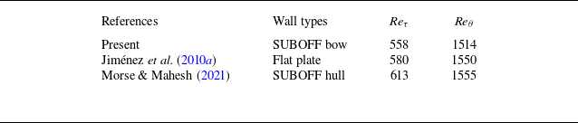
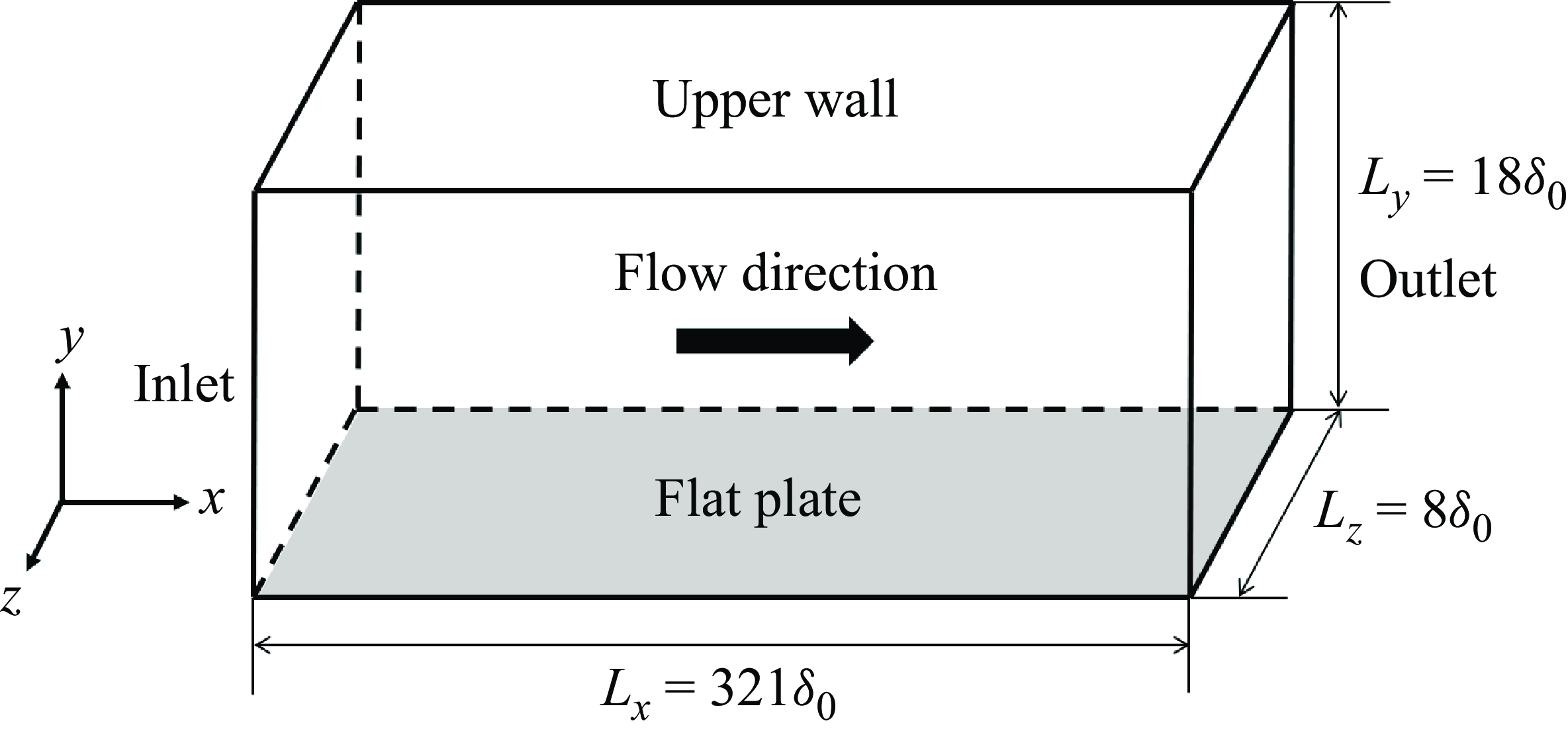
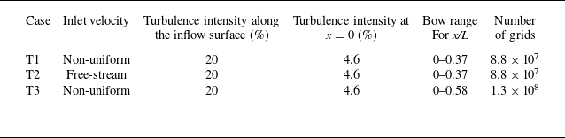
1. Introduction
The boundary layer flow over an axisymmetric body is of great significance in practical engineering applications. Underwater vehicles typically have a blunt axisymmetric body shape. Flow phenomena over an axisymmetric body are quite complicated at different sections, and are closely related to the hydrodynamic performances of vehicles, such as drag and noise. The evolutionary characteristics of flow along the straight section (Posa & Balaras Reference Posa and Balaras2016, Reference Posa and Balaras2020), the sail (Luo et al. Reference Luo, Sun, Zhang, Zhan and Cai2019; Liu et al. Reference Liu, Zhou, Zhu and Wang2021b ), the tail (Morse & Mahesh Reference Morse and Mahesh2021) and the wake (Jiménez et al. Reference Jiménez, Hultmark and Smits2010b , Reference Jiménez, Reynolds and Smits2010c ; Kumar & Mahesh Reference Kumar and Mahesh2018) were extensively investigated in previous studies. However, in the case of a bow with strong streamwise curvature, the focus has primarily been on the wall pressure fluctuation (WPF), with limited attention given to the boundary layer over the bow surface. In practice, interaction between the bow and the surrounding flow is the source of noise, leading to a reduction in the detection capability of sonar platforms and impeding the enhancement of the operating speed of underwater vehicles. Resolving this issue necessitates a comprehensive understanding of the flow characteristics within the bow boundary layer.
The boundary layer flow over an axisymmetric body was investigated by experimental and numerical methods. In the experimental studies, tests were performed in wind/water tunnels and deep lakes. The Submarine Technology Program Office (SUBOFF) model was proposed by the Defense Advanced Research Projects Agency (DARPA) as a benchmark model, which can be used to obtain the database for computational fluid dynamics (CFD) validation and other related flow field analyses of submarines. Huang & Liu (Reference Huang and Liu1994) conducted wind tunnel experiments by using the SUBOFF model with and without appendages, obtaining pressure and skin friction data along the hull. Trip wires were adopted at the middle of the bow to generate turbulence, and only field data in the thick boundary layer at the tail were obtained. In a wind tunnel, Jiménez et al. (Reference Jiménez, Hultmark and Smits2010b
, Reference Jiménez, Reynolds and Smits2010c
) measured the intermediate wake of SUBOFF. They found that, different from the Reynolds stress, there existed self-similarity for the mean velocity at all locations. In a high-speed water tunnel, Ladd (Reference Ladd1990) controlled the random Tollmien–Schlichting (T–S) waves by using a suction/blowing slot on an axisymmetric body. Miao et al. (Reference Miao, Li, Pang, Xiao and Jia2020) conducted water tunnel experiments with a cone-cylinder-hemisphere model and measured the WPF. Results showed that the WPF continued to increase as the free-stream velocity increased. Flow separation was more likely at positions where the shape changed abruptly. Recently, Liu et al. (Reference Liu, Pan and Liu2023b
, Reference Liu, Pan, Zhang and Liu2024) measured a transitional boundary layer around SUBOFF in a low-speed water tunnel. Wavelet transform analysis indicated that the intermittent behaviour of Reynolds shear stress existed mainly in the mid-to-high-frequency range. The quick amplification of small-scale motions led to the secondary streak instability. Moreover, Abarbanel et al. (Reference Abarbanel, Katz, Galib, Cembrola and Frison1994) conducted lake trials by using a buoyant axisymmetric vehicle at a Reynolds number of
 $\mathop {\textit{Re}}\nolimits _L\sim {10^8}$
, based on the free-stream velocity and the model length. Regions of laminar, transitional and turbulent flows were distinguished by nonlinear dynamics analysis. Spectra of WPF at different streamwise locations were measured. Wei et al. (Reference Wei, Yan, Liu, Liu, He and Sun2024) conducted lake trials to study the hydrodynamic characteristics of autonomous underwater vehicles. They found that the resistance generated by appendages significantly increased with the increase of inflow velocity.
In numerical investigations, for the flow over an axisymmetric body with a non-zero angle of attack, the vortical structures induced by the flow separation and the distributions of skin friction and pressure were investigated extensively (Yang & Lohner Reference Yang and Lohner2003; Gross et al. Reference Gross, Kremheller and Fasel2011, Reference Gross, Jagadeesh and Fasel2012; Abedi et al. Reference Abedi, Dehghan, Saeidinezhad and Manshadi2016). With a zero angle of attack, turbulence cannot be generated at a relatively low Reynolds number, and thus a trip wire or blowing was usually applied at the mid-bow to induce a rapid transition. Different numerical methods were applied, including Reynolds-averaged Navier–Stokes (RANS) equations (Kim et al. Reference Kim, Park, Van and Kim2003; Drouet et al. Reference Drouet, Reliquet, Bardin, Jacquin, Gentaz and Alessandrini2011; Lyu et al. Reference Lyu, Tang, Sun, Wu and Chen2014), detached eddy simulations (Alin et al. Reference Alin, Bensow, Fureby, Huuva and Svennberg2010; Lungu Reference Lungu2019) and large-eddy simulations (LES) (Posa & Balaras Reference Posa and Balaras2016; Kumar & Mahesh Reference Kumar and Mahesh2018; Shi et al. Reference Shi, Yang, Jin, He and Wang2019; Morse & Mahesh Reference Morse and Mahesh2021). In the streamline-normal coordinate system, Morse & Mahesh (Reference Morse and Mahesh2021) gave a new perspective on the analysis of the turbulent boundary layer (TBL) over the SUBOFF model. At the forebody of the model, the momentum equation in the streamline direction represents a balance of the streamwise advection, pressure gradient and viscous stress, while that in the normal direction represents a balance between the normal pressure gradient and centripetal acceleration. At the straight section, the evolution of the TBL was quite similar to that over a flat plate, owing to the small pressure gradient and large spanwise radius, which was also pointed out by Posa & Balaras (Reference Posa and Balaras2016, Reference Posa and Balaras2020). However, Kumar & Mahesh (Reference Kumar and Mahesh2018) found that, compared with a planar TBL, the axisymmetric TBL had higher skin friction and higher radial decay of turbulence away from the wall. At the stern, where the TBL was very thick, Morse & Mahesh (Reference Morse and Mahesh2021) found that the curvature and streamwise-pressure-gradient terms could not be ignored and appeared to balance the turbulent and viscous stresses. In the wake region, Kumar & Mahesh (Reference Kumar and Mahesh2018) pointed out that the turbulent intensities were not self-similar. Plasseraud, Kumar & Mahesh (Reference Plasseraud, Kumar and Mahesh2023) employed LES to compute the flow around a prolate spheroid with a non-zero angle of attack, exploring the influence of the trip on the boundary layer flow state. It was discovered that, although the trip accelerates the transition to turbulence, it does not induce a fully developed TBL as expected, even at a significant angle of attack of 20
 $^\circ$
. More recently, Morse & Mahesh (Reference Morse and Mahesh2023) further investigated the influence of trips based on the SUBOFF model. They found that when the size of the trip exceeds the thickness of the laminar boundary layer, the vortex shedding from the trip can initiate flow transition, resulting in a significant jump in the boundary layer thickness. The lasting impact of the trip is the change of boundary layer thickness caused by it, and as the TBL grows, the proportion of this change gradually decreases. Posa & Balaras (Reference Posa and Balaras2016, Reference Posa and Balaras2020) also observed a bimodal behaviour for the turbulent stresses in the wake, which was enhanced by the interaction of the boundary layer with the leading edge of the fins. However, in the above numerical studies, the flow characteristics of the front area of the bow were usually not discussed.
As a related problem, turbulent flow over a curved wall has been extensively investigated. El-Askary (Reference El-Askary2009) and Bentaleb, Lardeau & Leschziner (Reference Bentaleb, Lardeau and Leschziner2012) employed the LES method to investigate the effect of a convex curved wall on flow separation, reattachment and coherent structures. El-Askary (Reference El-Askary2009) found that in the region of adverse pressure gradient generated by the curved wall, vortices exhibit strong elongation and lift. Bentaleb et al. (Reference Bentaleb, Lardeau and Leschziner2012) observed that the separation process is highly unsteady in both time and space, and the turbulence exhibits non-local characteristics. Wu & Squires (Reference Wu and Squires1998) and Balin & Jansen (Reference Balin and Jansen2021) simulated the boundary layer flow on a convex wall using the LES method and direct numerical simulation (DNS) method, respectively. Wu & Squires (Reference Wu and Squires1998) found that, although the flow experiences a strong adverse pressure gradient along the rear surface, the intermittent separation occurring near the wall is not accompanied by the separation of the mean flow. Balin & Jansen (Reference Balin and Jansen2021) showed that the strong adverse pressure gradient causes the boundary layer to enter a re-laminarisation process, with near-wall turbulence significantly weakening and becoming intermittent, but the re-laminarisation is incomplete. Moser & Moin (Reference Moser and Moin1987) and Brethouwer (Reference Brethouwer2022) investigated the fully developed turbulent flow characteristics in curved channels through the DNS method. Moser & Moin (Reference Moser and Moin1987) found the presence of Taylor–Gortler vortices in low Reynolds number flows. Brethouwer (Reference Brethouwer2022) reported that, at higher Reynolds numbers, the flow undergoes local re-laminarisation near the convex wall under the strongest curvature conditions. On the concave side, large elongated vortices similar to Taylor–Gortler vortices are formed. In addition, Pargal et al. (Reference Pargal, Wu, Yuan and Moreau2022) and Caiazzo et al. (Reference Caiazzo, Pargal, Wu, Sanjosé, Yuan and Moreau2023) studied the TBL on the suction surface of airfoils. Pargal et al. (Reference Pargal, Wu, Yuan and Moreau2022) found that in regions with weaker pressure gradients or thicker boundary layers, the effects of wall curvature and adverse pressure gradient interact with each other. Caiazzo et al. (Reference Caiazzo, Pargal, Wu, Sanjosé, Yuan and Moreau2023) demonstrated that the presence of a strong adverse pressure gradient significantly enhances the intensity of low-frequency WPFs, shortens the downstream coherence of WPF in time and space and expands the spanwise coherence, but significantly reduces the convective velocity. In the present study, the bow of the SUBOFF model can be regarded as a convex wall with a strong favourable pressure gradient at the front part, while the flow transition should also be of concern under the effects of a favourable pressure gradient and incoming turbulent flow.
For the flow over a bow, features of the transition and flow separation, and shape design, have always been focused on. The optimisation design of bow shapes was explored by CFD analysis (Yazici Reference Yazici2020). The hydrodynamic features and the noise were both sensitive to the shape of the forebody. By comparing the hydrodynamic performances of different models, Moonesun et al. (Reference Moonesun, Korol, Nikrasov, Ursalov and Brajhko2016a
, Reference Moonesun, Mahdian, Korol, Dadkhah and Javadi2016b
) concluded that a blunt shape should be recommended rather than the sharp narrow one. Lauchle’s sound radiation theory was applied to calculate the noise caused by the flow over a bow (Li, Zhang & Shi Reference Li, Zhang and Shi1999; Yu, Lv & Wu Reference Yu, Lv and Wu2002; Lv, Jin-lin & Xiao-wei Reference Lv, Miao and Zhang2012). Accordingly, shapes of the forebody were designed to achieve the low noise condition. The profile of the optimised model was between the sharp and blunt ones, consistent with the conclusion of Blake (Reference Blake2017). Hong et al. (Reference Hong, Shin, Jeon and Kim2008) conducted wind tunnel experiments at a Reynolds number of
 ${\mathop {\textit{Re}}\nolimits } _s = 3{-}6 \times {10^5}$
, based on the free-stream velocity and the arc length. They found that the spectra of WPF in the transition region were scaled well by the outer variables due to the existence of large-scale Tollmien–Schlichting waves. In the transition region, Hong (Reference Hong2015) detected a slope of −8/3 in the log–log scale in the high-frequency region of the pressure spectra. Wind tunnel tests were also executed to investigate the characteristics of pressure spectra in the laminar separation region in Lee et al. (Reference Lee, Kim, Kwon and Lee2000). They found that, owing to the hemispherical nose, the laminar separation was produced and the induced WPF was 4–5 times larger than that in the transition region. The prediction of the boundary layer transition is also a key area of focus. The Granville method was used to find the position of transition, which was validated in numerous boundary layer calculations (Zhao, Shi & Du Reference Zhao, Shi and Du2008). Liu et al. (Reference Liu, Chu and Zhang2021a
) studied the natural transition over bows with different shapes by the eN method based on stability analysis. The eN method is a semi-empirical method related with linear flow stability theory, which is used to predict the natural transition location of the boundary layer flow. The results showed that, for a given bow shape, the transition location was sensitive to the change of Reynolds number at a relatively low speed. The SUBOFF model had distinct advantages in practical applications, due to the late transition and the relatively large diameter at the front of the bow. The effect of Reynolds number was then investigated by the eN method in Liu et al. (Reference Liu, Liu and Zhang2023a
), which was strongly nonlinear. For the forebody shapes adopted in their research, improved shapes were reported to have a later transition position than the SUBOFF bow at a certain Reynolds number, which gave inspiration to the transition delay. For the axisymmetric bow at an angle of incidence to the free-stream velocity, flow separation may occur, and the wall pressure and skin friction coefficients undergo significant changes, thereby significantly altering the hydrodynamic and noise characteristics of the bow. Based on the velocity profiles of Laser Doppler Velocimetry, the wall shear stress on a prolate spheroid exhibited three-dimensional (3-D) flow separation characteristics, which was different with the two-dimensional (2-D) flow separation (Chesnakas & Simpson Reference Chesnakas and Simpson1997). The local minimum wall shear stress was located further downstream. Pantelatos & Mathioulakis (Reference Pantelatos and Mathioulakis2004) conducted measurement experiments for static pressure, wall shear stress and velocity on blunt bows at different angles of attack, as well as flow visualisation. Due to the low Reynolds number, an axisymmetric flow phenomenon was observed. Lee & Jones (Reference Lee and Jones2020) conducted wall pressure measurements on blunt bodies with angles of attack at high Reynolds numbers. They found that the separation envelope is located in the plateau region in the circumferential distribution of the average pressure. Pattern tracking indicated that the trajectory of the maximum circumferential pressure gradient was similar to the separation trajectory, but was located further upstream of the body.
In summary, the previous experimental studies primarily focused on investigating wall pressure on the bow. For the numerical simulations, trip wires were applied at the bow to induce turbulence, and the main emphasis was usually directed towards analysing the flow at the straight section, the tail of the model and the wake, where capturing fine structures was relatively feasible. However, a comprehensive investigation into the statistical properties of the boundary layer over the bow is still lacking. Given that there is a pronounced streamwise curvature for the bow, understanding its impact on flow characteristics in comparison with flat-plate flow remains elusive. Furthermore, considering complex sea environments and aiming for more realistic simulations of practical situations, it becomes imperative to incorporate turbulent inflow. The influence of inflow turbulence intensity (ITI) continues to be an area yet unexplored.
In the present study, the wall-resolved LES is applied to simulate the flow over the bow of the axisymmetric SUBOFF model. We aim to answer the following questions. Firstly, what are the characteristics of the curved-edge boundary layer over the bow and its differences from the flat-plate boundary layer? Secondly, what are the influences of ITI? The free-stream Reynolds number is
 $\mathop {\textit{Re}}\nolimits _L = 1.1 \times {10^6}$
, the same as that in Kumar & Mahesh (Reference Kumar and Mahesh2018). To excite the generation of turbulence within the boundary layer, the isotropic turbulent inflow condition is considered. The statistical properties of the boundary layer over a blunt bow and the influences of geometric curvature and ITI on evolutionary features of TBL are examined in detail. The paper is organised as follows. The numerical method, the set-up for the simulation including the geometry of the computational domain, the boundary conditions and the grid resolution, generation method of turbulent inflow and an overview of the axisymmetric bow-profile coordinate system and related equations are introduced in § 2. Results of different cases are presented and discussed in §§ 3–6. Finally, conclusions are drawn in § 7.
2. Computational approaches
2.1. Numerical set-up
The present wall-resolved LES is performed by solving the spatially filtered Navier–Stokes (N–S) equations for incompressible Newtonian flow
 \begin{align} \left . \begin{array}{c} \dfrac {{\partial {{\tilde u}_i}}}{{\partial t}} + \dfrac {{\partial ( {{{\tilde u}_i}{{\tilde u}_j}} )}}{{\partial {x_j}}} = - \dfrac {{\partial \tilde p}}{{\partial {x_i}}} + \dfrac {1}{\textit{Re}}\dfrac {{{\partial ^2}{{\tilde u}_i}}}{{\partial {x_j}\partial {x_j}}} - \dfrac {{\partial {\tau _{\textit{ij}}}}}{{\partial {x_j}}},\\ \dfrac {{\partial {{\tilde u}_i}}}{{\partial {x_i}}} = 0, \end{array} \right \} \end{align}
where
 $u_i$
is the velocity,
 $p$
is the pressure and
 $\textit{Re} = {{{U_\infty }L} / \nu }$
is the Reynolds number, with
 $U_\infty$
denoting the free-stream velocity,
 $L$
the length of SUBOFF model and
 $\nu$
the kinematic viscosity. The summation convention is applied with
 $i,j=1,2,3$
. Note that (2.1) are solved based on the Cartesian coordinate system. The symbol
 $\widetilde { ( \boldsymbol{\cdot })}$
denotes the spatial filtering, and for the sake of simplicity, this symbol will not appear in subsequent parameters. The sub-grid stress
 $\tau _{\textit{ij}} = \widetilde {{u_i}{u_j}} - {\tilde u_i}{\tilde u_j}$
is parameterised by the wall-adapting local eddy-viscosity model (Nicoud & Ducros Reference Nicoud and Ducros1999). Based on the Pressure implicit with splitting of operators algorithm in OpenFOAM, the governing equations are solved using the finite-volume method. The backward scheme is adopted for time integration (Jasak Reference Jasak1996), i.e.
 \begin{equation} \frac {{\partial {u_i}}}{{\partial t}} = \frac {1}{{\Delta t}}\left ( {\frac {3}{2}{{\left . {{u_i}} \right |}_{t + 1}} - 2{{\left . {{u_i}} \right |}_t} + \frac {1}{2}{{\left . {{u_i}} \right |}_{t - 1}}} \right )\!. \end{equation}
Spatial derivatives are discretised by the second-order central-difference scheme. Note that for the discretisation of the convective term, the improved Total Variation Diminishing scheme is applied to eliminate numerical oscillations.
A 3-D axisymmetric domain is used for simulation of flow over a SUBOFF bow, as shown in figure 1(a). For convenience, three coordinate systems are used in the following. One is the Cartesian coordinate system (
 $x,y,z$
), or equivalently (
 $x_1, x_2, x_3$
). The second one is the cylindrical coordinate system (
 $x,r,\theta$
), representing the coordinates in the streamwise, radial and spanwise directions, respectively. The third one is the axisymmetric bow-profile coordinate system (
 $s,n,\theta$
), representing the arc/tangential, wall-normal and spanwise directions, respectively. The axisymmetric bow-profile coordinate system is orthogonal, thus the equations in (
 $s,n,\theta$
) can be simplified from a general curvilinear coordinate system. More details about the axisymmetric bow-profile coordinate system are introduced in § 2.3. The origin of the coordinate systems is located at the nose of the bow. The distance from the inlet to the nose of the bow is 3.6R, where R is the maximum radius of the bow. By plotting the normal lines from the bow surface with an equal height of 3.6R, the inlet surface can be obtained. Here, a 1/120-scale SUBOFF model with R = 0.0508 and R = 0.8712 m is used, which is the same as that in the experiment of Jimenez et al. (Reference Jiménez, Hultmark and Smits2010b
). The bow radius (r) can be expressed as follows (Groves, Huang & Chang Reference Groves, Huang and Chang1989):
 \begin{equation} r = \begin{cases} R\left \{ {\dfrac {{1.126395101x}}{{0.06096}}{{\left ( {\dfrac {{0.3x}}{{0.06096}} - 1} \right )}^4}} \right . \\{\text{ }} + 0.442874707{\left ( {\dfrac {x}{{0.06096}}} \right )^2}{\left ( {\dfrac {{0.3x}}{{0.06096}} - 1} \right )^3} \\{\text{ }} + {\left . {1 - \left ( {\dfrac {{1.2x}}{{0.06096}} + 1} \right ){{\left ( {\dfrac {{0.3x}}{{0.06096}} - 1} \right )}^4}} \right \}^{{1 / {2.1}}}},x \lt 0.2032{m} \\R,x \geqslant 0.2032{m}. \end{cases} \end{equation}
The relatively small domain may bring the confinement effect. Thus, to avoid it, spatially variant velocities are employed along the inflow surface, as plotted in figure 1(b), rather than a uniform free-stream velocity
 $U_{\infty }$
. The profiles are obtained from the LES of 2-D axisymmetric flow over the bow in a large domain. In this 2-D simulation, a uniform free-stream velocity
 $U_{\infty }$
is applied along the inflow surface, and the domain is two orders of magnitude larger than that of Kumar & Mahesh (Reference Kumar and Mahesh2018). Then the inflow condition is given as
 $U_x = {U_{x,2D}}$
,
 $U_y = {U_{r,2D}}\cos \theta$
and
 $U_z = {U_{r,2D}}\sin \theta$
. No-slip condition is applied at the bow surface and constant-pressure condition is used at the outlet.
Computational settings: (a) schematic of computational domain and boundary conditions; (b) mean velocity profiles along the inflow surface; (c) schematic of grid subdivision for the bow surface and the x–y plane.

To deal with the singularity of the cylindrical coordinate system when the radius tends to zero (O’Sullivan & Breuer Reference O’sullivan and Breuer1994), an O-block mesh (shown in figure 1
c) is constructed in the present simulations, instead of a rotationally symmetric one. Simulations of flow over the SUBOFF bow are preformed at a Reynolds number of
 $\textit{Re}{_L} = 1.1 \times {10^6}$
. The grid sizes at the bow surface satisfy
 $\Delta {s^ + } \lt 24$
and
 $r\Delta {\theta ^ + } \lt 12$
, and the first wall-normal grid resolution satisfies
 $\Delta n_w^ + \lt 1$
. In total 570–870 million grids are used. The computational time step is
 $\Delta t \times {{{U_\infty }} / L} = 2.7 \times {10^{ - 4}}$
, ensuring that the maximum local Courant number is less than 1. After reaching the statistically steady state, the data over fifteen flow-through-body times are then used to compute the statistics.
Details for the numerical validation can be found in Appendices A and B, and verification of the inlet/outlet computational settings can be found in Appendix C.
2.2. Generation of turbulent inflow
To induce flow transition in the boundary layer over the bow, a turbulent flow field is artificially pre-generated and serves as the inflow condition (figure 1 a). The Kraichnan technique (Saad et al. Reference Saad, Cline, Stoll and Sutherland2017) is adopted to generate the isotropic turbulent flow field, which is supposed to satisfy the von Karman–Pao spectrum (Bailly & Juve Reference Bailly and Juve1999), i.e.
 \begin{equation} E(\kappa ) = a \frac {{u_{\textit{rms}}^{\prime 2}}}{{{\kappa _e}}}\frac {{{{\left ( {\kappa /{\kappa _e}} \right )}^4}}}{{{{\left [ {1 + \left ( {\kappa /{\kappa _e}} \right )} \right ]}^{17/6}}}}\exp \! \left [ { - 2{{\left ( {\frac {\kappa }{{{\kappa _\eta }}}} \right )}^2}} \right ]\!,a \approx 1.453, \end{equation}
where
 $u'_{\textit{rms}}$
is the root mean square of the velocity fluctuation,
 $\kappa$
is the wavenumber,
 $\kappa _e$
is related to the integral length scale
 $L \approx {{0.747} / {{\kappa _e}}}$
and
 $\kappa _\eta$
is the corresponding wavenumber for the Kolmogorov scale. Note that the turbulence intensity
 $I=u'_{\textit{rms}}/U_{\infty }$
also serves as an input parameter in (2.4). Velocities are reconstructed based on the spectrum model
 \begin{equation} {\boldsymbol{u}}({\boldsymbol{x}}) = 2\sum \limits _{m = 1}^M {{q_m}} \cos \! \left ( {{\kappa _m}{{\widehat {\boldsymbol{k}}}_m} \boldsymbol{\cdot }{\boldsymbol{x}} + {\psi _m}} \right ){\widehat {{\sigma }}_m},{q_m} = \sqrt {E\left ( {{\kappa _m}} \right )\Delta \kappa }, \end{equation}
where
 $M$
is the mode number,
 $\kappa _m$
is the wavenumber,
 $\widehat {\boldsymbol{k}}_m$
is the unit direction vector related with
 $\kappa _m$
,
 $\boldsymbol{x}$
is the coordinate of discrete points,
 $\psi _m$
is the random phase angle and
 $\widehat {{\sigma }}_m$
is the unit direction vector used to compulsively satisfy the divergence-free condition in the entire flow field. As a result, the energy spectrum of the generated turbulent flow field agrees well with the theoretical expression (2.4), as shown in figure 2(a). The contours of streamwise velocity are displayed in figure 2(b). The Kraichnan method has been widely applied in generating the initial flow field (Chung, Mishra & Ihme Reference Chung, Mishra and Ihme2022; Chen et al. Reference Chen, Li, Wang, Hu and Xiao2024; Idelsohn, Gimenez & Onate Reference Idelsohn, Gimenez, Larreteguy, Nigro, Sívori and Oñate2024) and turbulent inflow (Markesteijn & Karabasov Reference Markesteijn and Karabasov2019; Markesteijn et al. Reference Markesteijn, Gryazev, Karabasov, Ayupov, Benderskiy and Lyubimov2020), where good agreements with experimental data can be found.
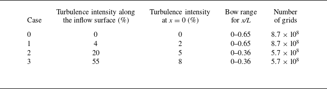
Computational parameters for different cases. Higher turbulence intensity level is given to achieve the target level at the x = 0 plane.

(a) Energy spectrum of synthetic turbulence and (b) streamwise velocity for the isotropic turbulent field by using Kraichnan’s technique.

Based on the generated isotropic velocity fluctuations, by adding the mean values in figure 1(b), Taylor’s frozen hypothesis is then utilised to transform the streamwise velocity into signals in the temporal direction. The generated flow data are then enforced as the turbulent inflow within the region
 $r \leqslant 1.4R$
. The Heaviside function (2.6) is adopted to transit from the turbulence region to the free-stream region at
 $r = 1.4R$
(Chang et al. Reference Chang, Hou, Merriman and Osher1996), i.e.
 \begin{equation} \phi = {H_{\alpha _d} }(d) = \left \{ \begin{array}{l} 1,d \gt \alpha _d ,\\[4pt]0,d \lt - \alpha _d ,\\[4pt]\dfrac {1}{2} \left(1 + \dfrac {d}{\alpha _d } + \dfrac {1}{\pi }\sin \left(\dfrac {{\pi d}}{\alpha _d }\right)\right)\,{\rm otherwise}, \end{array} \right . \end{equation}
where
 $d = r - 1.4R$
is the distance from the interface
 $r = 1.4R$
, and
 $\alpha _d$
is the width for the transition area. Here,
 $\alpha _d/R\approx 0.1$
is used. Then, the turbulence intensity is expressed as
 $I = {I_0}\phi$
at the inflow region, where
 $I_0$
is the prescribed ITI.
As seen in table 1, four cases with different inflow turbulent intensities ranging from 0 % to 55 % are simulated. Before encountering the bow (
 $x/L \lt 0$
), the flow can be regarded as homogeneous turbulence that decays exponentially downstream. By adjusting the turbulence intensity at the inflow surface, the turbulence intensities within
 $r/R=0.6{-}1.1$
at the
 $x = 0$
plane of 0 %, 2 %, 5 % and 8 % are chosen as cases 0–3, respectively, as listed in table 1. The previous studies showed that the incoming flow field of a navigating submarine in a real underwater environment is very complex, with measured turbulence intensities ranging from 0.03 % to 7 % (Osborn Reference Osborn1978; Reference Osborn1980; Witte et al. Reference Witte, Brattegard, Graf and Springer1997; Gargett Reference Gargett1999; Greene, Hendricks & Gregg Reference Greene, Hendricks and Gregg2015). Therefore, this study focuses on the flow around SUBOFF with incoming turbulence intensities ranging from 0 % to 8 % at x = 0. The turbulent integral length scale at the inflow in all cases is set to be 0.06R, which is within the range of integral scales under real sea conditions (Bouruet-Aubertot et al. Reference Bouruet-Aubertot, Cuypers, Ferron, Dausse, Ménage, Atmadipoera and Jaya2018). Moreover, for the flow to develop fully downstream, the bow length in cases 0 and 1 is larger than that in cases 2 and 3.
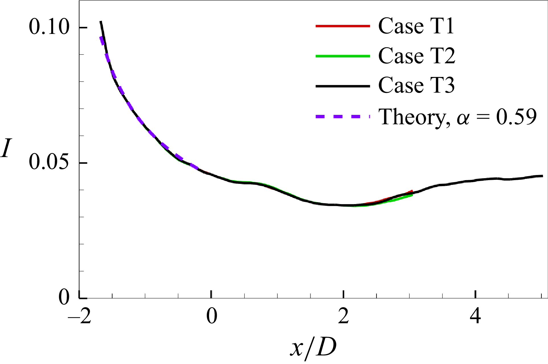
In figure 3(a), variations of the turbulence intensity in cases 1–3 with the streamwise position are plotted. In each case, the results at different radius positions (
 ${r / R} = 0{-}1.1$
) collapse well with the theoretical one, demonstrating the homogeneity of turbulence in the incoming flow region. According to the classical theory of isotropic turbulence (Saffman Reference Saffman1967), the turbulence intensity
 $I$
varies as
 $I \sim { ( {x - {x_{\textit{inlet}}}} )^{ - \alpha }}$
, where
 $x$
is the distance along the downstream evolution,
 $x_{\textit{inlet}}$
is the streamwise location of the inlet region and
 $\alpha$
is the attenuation factor. In cases 1–3, the factor
 $\alpha$
is within the scope given in Saffman (Reference Saffman1967). In figure 3(b), the pressure spectra in the incoming flow region are presented. Specifically, the scaling law
 ${\varPhi _{pp}} ( \omega ) \sim {\omega ^{{{ - 7} / 3}}}$
is observed in the mid-frequency region, which is a typical feature of homogeneous turbulence (Gotoh & Fukayama Reference Gotoh and Fukayama2001).
Characteristics of incoming turbulence evolution: (a) turbulence intensity at different radial positions; (b) pressure spectra at different streamwise positions, scaled by the outer scales. The non-dimensional spectra are represented by
 ${{{\varPhi _{pp}}D} /{( {p_{\textit{rms}}^{\prime 2}U} )}}$
versus
 ${\omega D} / U$
, where
 $D$
is the maximum diameter of the bow,
 $U$
is the local mean streamwise velocity,
 $ \omega$
is the angular frequency and
 $p'_{\textit{rms}}$
is the root mean square of the local pressure fluctuation.

2.3. Expressions in the axisymmetric bow-profile coordinate system
For facilitating analysis in the following sections, the axisymmetric bow-profile coordinate system (
 $s,n,\theta$
) is used. The velocity components
 ${u_i} ( {i = s,n,\theta } )$
are projected along the curvilinear coordinate lines. The N–S equations in the (
 $s,n,\theta$
) coordinates can be written as follows:
 \begin{align} & \frac {{\partial {u_i}}}{{\partial t}} + {u_i}\frac {{\partial {u_i}}}{{\partial {\xi _i}}} + {u_j}\frac {{\partial {u_i}}}{{\partial {\xi _j}}} + {u_k}\frac {{\partial {u_i}}}{{\partial {\xi _k}}} + {K_{\textit{ij}}}{u_i}{u_j} - {K_{\textit{ji}}}{u_j}{u_j} + {K_{\textit{ik}}}{u_i}{u_k} - {K_{\textit{ki}}}{u_k}{u_k}\nonumber \\& = - \frac {\partial }{{\partial {\xi _i}}}\left ( {\frac {p}{\rho }} \right ) + \nonumber \\& \nu \left \{ {{{\nabla} ^2}{u_i} + 2{K_{\textit{ij}}}\frac {{\partial {u_j}}}{{\partial {\xi _i}}} + 2{K_{\textit{ik}}}\frac {{\partial {u_k}}}{{\partial {\xi _i}}} - 2{K_{\textit{ji}}}\frac {{\partial {u_j}}}{{\partial {\xi _j}}} - 2{K_{\textit{ki}}}\frac {{\partial {u_k}}}{{\partial {\xi _k}}} + {\alpha _{\textit{ii}}}{u_i} + {\alpha _{\textit{ij}}}{u_j} + {\alpha _{\textit{ik}}}{u_k}} \right \}\nonumber \\& \frac {{\partial {u_i}}}{{\partial {\xi _i}}} + \frac {{\partial {u_j}}}{{\partial {\xi _j}}} + \frac {{\partial {u_k}}}{{\partial {\xi _k}}} + \left ( {{K_{\textit{ji}}} + {K_{\textit{ki}}}} \right ){u_i} + \left ( {{K_{\textit{ij}}} + {K_{\textit{kj}}}} \right ){u_j} + \left ( {{K_{\textit{ik}}} + {K_{\textit{jk}}}} \right ){u_k} = 0 , \end{align}
where
 $i,j,k=s,n,\theta$
and
 ${\partial / {\partial {\xi _s}}} = {\partial / { ( {{h_s}\partial s} )}}$
,
 ${\partial / {\partial {\xi _n}}} = {\partial / { ( {{h_n}\partial n} )}} = {\partial / {\partial n}}$
and
 ${\partial / {\partial {\xi _\theta }}} = {\partial / { ( {{h_\theta }\partial s} )}}$
. Here,
 $K_{\textit{ij}}$
and
 $\alpha _{\textit{ij}}$
are parameters related to the Lame coefficient
 $h_i$
(Richmond, Chen & Patel Reference Richmond, Chen and Patel1986) as follows:
 \begin{equation} {K_{\textit{ij}}} = \frac {1}{{{h_i}}}\frac {{\partial {h_i}}}{{\partial {\xi _j}}},{\alpha _{\textit{ij}}} = \frac {{\partial {K_{\textit{ij}}}}}{{\partial {\xi _i}}} - \frac {{\partial {K_{\textit{ji}}}}}{{\partial {\xi _j}}} - {K_{\textit{kj}}}\left ( {{K_{\textit{ki}}} + {K_{\textit{ji}}}} \right ) + {K_{\textit{ki}}}{K_{\textit{ij}}}. \end{equation}
Note that the repeated subscripts in (2.7) and (2.8) do not conduct the summation operation. More details can be found in Appendix D.
To understand the generation mechanism of skin friction, the dynamic decomposition of the skin friction coefficient
 $C_f$
can be derived by double integrations of the Reynolds-averaged form of (2.7). Here,
 $C_f$
is defined as
 ${C_f} = {{{\tau _w}} / { ( {0.5\rho U_\infty ^2} )}}$
, where
 $\tau _w$
is the local wall shear stress at the bow surface, and
 $U_{\infty }$
is the free-stream velocity, which is used at the inlet for LES of 2-D axisymmetric flow over the bow in a large domain, as mentioned in § 2.1. The dynamic decomposition of
 $C_f$
is expressed as follows:
 \begin{align} & {C_f} = \underbrace {\frac {2}{{{\textit{Re}_\delta }}}{{\left . {{U_s}} \right |}_{{\delta _{99}}}}\beta }_{{C_{\nu 1}}}\underbrace { - \frac {4}{\textit{Re}}\left ( {\beta - 1} \right )\int _0^1 {{U_s}{\rm d}n} }_{{C_{\nu 2}}}\underbrace { - 2\int _0^1 {\frac {r}{{{{\left . r \right |}_0}}}\overline {{{u'}_s}{{u'}_n}} {\rm d}n} }_{{C_R}} \nonumber\\& \underbrace { - 2 \! \int _0^1 \!\! {\left ( {1 - n} \right )\!\left (\! {{U_s}\frac {1}{h_s}\frac {{\partial {U_s}}}{{\partial s}} + {U_n}\frac {{\partial {U_s}}}{{\partial n}}} \! \right )\!{\rm d}n} }_{{C_{C1}}}\underbrace { - 2 \!\left ( {\beta - 1} \right ) \!\int _0^1 \!\! {\big ( {1 - {n^2}} \big ) \!\left ( \! {{U_s}\frac {1}{h_s}\frac {{\partial {U_s}}}{{\partial s}} + {U_n}\frac {{\partial {U_s}}}{{\partial n}}} \! \right ){\rm d}n} }_{{C_{C2}}}\nonumber\\& \underbrace { - 2\int _0^1 {\left ( {1 - n} \right )\frac {1}{h_s}\frac {{\partial P}}{{\partial s}}{\rm d}n} }_{{C_{P1}}}\underbrace { - 2\left ( {\beta - 1} \right )\int _0^1 {\big( {1 - {n^2}} \big)\frac {1}{h_s}\frac {{\partial P}}{{\partial s}}{\rm d}n} }_{{C_{P2}}}\nonumber\\& + \underbrace {2\int _0^1 {\left ( {1 - n} \right )\left ( {\frac {1}{{{\textit{Re}}}}{{\nabla} ^2}{U_s} - \frac {1}{{{\textit{Re}}}}\frac {{{\partial ^2}{U_s}}}{{\partial {n^2}}} + \frac {1}{h_s}\frac {{\partial \overline {{{u'}_s}{{u'}_s}} }}{{\partial s}}} \right ){\rm d}n} }_{{C_{D1}}}\nonumber\\& + \underbrace {2\left ( {\beta - 1} \right )\int _0^1 {\big( {1 - {n^2}} \big)\left ( {\frac {1}{{{\textit{Re}}}}{{\nabla} ^2}{U_s} - \frac {1}{{{\textit{Re}}}}\frac {{{\partial ^2}{U_s}}}{{\partial {n^2}}} + \frac {1}{h_s}\frac {{\partial \overline {{{u'}_s}{{u'}_s}} }}{{\partial s}}} \right ){\rm d}n} }_{{C_{D2}}} + {C_{f,\textit{geo}}}, \end{align}
where
 $U_i$
is the mean velocity,
 $u'_i$
is the velocity fluctuation,
 $P$
is the mean pressure,
 ${\mathop {\textit{Re}_\delta }\nolimits } = {{{U_\infty }{\delta _{99}}} / \nu }$
, with
 $\delta _{99}$
the nominal thickness of boundary layer on the bow surface, and
 $\beta = {{{{\left . r \right |}_{{\delta _{99}}}}} / {{{\left . r \right |}_0}}}$
denotes the ratio of the radius at the outer edge of the boundary layer to that of the bow surface. The symbol
 $\left . {} \right |_0$
represents the value at the wall (
 $n = 0$
) and
 $\overline { ( \boldsymbol{\cdot })}$
denotes the average operation. Moreover, the terms containing the geometric parameters
 $K_{\textit{ij}}$
as defined in (2.8) are collected in
 $C_{f,\textit{geo}}$
, i.e.
 \begin{align} & {C_{f,\textit{geo}}} = - 2\int _0^1 {\left ( {1 - n} \right ){K_{\textit{sn}}}{U_s}{U_n}{\rm d}n} \nonumber \\& - 2\left ( {\beta - 1} \right )\int _0^1 {\big( {1 - {n^2}} \big){K_{\textit{sn}}}{U_s}{U_n}{\rm d}n} \nonumber \\& - 2\int _0^1 {\left ( {1 - n} \right )\big [ {\left ( {2{K_{\textit{sn}}} + {K_{\theta n}}} \right )\overline {{{u'}_s}{{u'}_n}} + {K_{\theta s}}\overline {{{u'}_s}{{u'}_s}} - {K_{\theta s}}\overline {{{u'}_\theta }{{u'}_\theta }} } \big ]{\rm d}n} \nonumber \\& - 2\left ( {\beta - 1} \right )\int _0^1 {\big( {1 - {n^2}} \big)\big [ {\left ( {2{K_{\textit{sn}}} + {K_{\theta n}}} \right )\overline {{{u'}_s}{{u'}_n}} + {K_{\theta s}}\overline {{{u'}_s}{{u'}_s}} - {K_{\theta s}}\overline {{{u'}_\theta }{{u'}_\theta }} } \big ]{\rm d}n} \nonumber\\& + \frac {2}{{{\text{Re}}}}\int _0^1 {\left ( {1 - n} \right )\left ( {2{K_{\textit{sn}}}\frac {{\partial {U_n}}}{{\partial s}} + {\alpha _{\textit{nn}}}{U_s} + {\alpha _{\textit{sn}}}{U_n}} \right ){\rm d}n} \nonumber\\& + \frac {2}{{{\text{Re}}}}\left ( {\beta - 1} \right )\int _0^1 {\big( {1 - {n^2}} \big)\left ( {2{K_{\textit{sn}}}\frac {{\partial {U_n}}}{{\partial s}} + {\alpha _{\textit{nn}}}{U_s} + {\alpha _{\textit{sn}}}{U_n}} \right ){\rm d}n}. \end{align}
Details of the derivation can be found in Appendix E. This decomposition formulation is an extension of that developed by Xia et al. (Reference Xia, Huang, Xu and Cui2015), which is based on the Cartesian coordinate system. Note that this expression is different from the Fukagata-Iwamoto-Kasagi (FIK) formulation (Fukagata, Iwamoto & Kasagi Reference Fukagata, Iwamoto and Kasagi2002), which is obtained by triple integrations in the wall-normal direction, in order to relate
 $C_f$
to the mean streamwise velocity. Accordingly, the FIK method is appropriate for situations with constant flow rate, while the present formulation is more suitable for cases of a given external flow velocity (Xia et al. Reference Xia, Huang, Xu and Cui2015).
As dictated in (2.9), the skin friction coefficient in the (
 $s,n,\theta$
) system can be decomposed into six parts: contributions from the viscous term, the development of external flow velocity and the flow rate,
 $C_{\nu 1}$
and
 $C_{\nu 2}$
; contribution from the Reynolds shear stress,
 $C_R$
; contributions from the mean convection terms,
 $C_{C1}$
and
 $C_{C2}$
; contributions from the mean-pressure-gradient terms,
 $C_{P1}$
and
 $C_{P2}$
; contributions from the derivatives of other terms,
 $C_{D1}$
and
 $C_{D2}$
; contribution from the direct geometric influence related to parameters
 $K_{\textit{ij}}$
,
 $C_{f,\textit{geo}}$
. Specifically, for the TBL flow over a flat plate, in term
 $C_R$
the values of
 $r$
and
 ${{\left . r \right |}_0}$
are equal;
 $\beta =1$
and
 $C_{\nu 2}$
,
 $C_{C2}$
,
 $C_{P2}$
and
 $C_{D2}$
are equal to zero; the geometric parameters
 $K_{\textit{ij}}=0$
, and thus
 $C_{f,\textit{geo}}$
is equal to zero. The detailed analysis of the contribution terms in (2.9) will be presented in § 5.
For the budget analysis in the curvilinear coordinate system, Richmond et al. (Reference Richmond, Chen and Patel1986) derived a general form of the Reynolds stress transport equations. However, their equations cannot express the impact of geometric curvature on energy transfer in the different budget terms. To separate the geometric and non-geometric influences, the Reynolds stress transport equations are derived from another perspective. Details of the derivation can be found in Appendix F. In a general curvilinear coordinate system, the Reynolds stress transport equations are expressed as follows:
 \begin{equation} \begin{array}{l} \underbrace {\frac {{\partial \big ( {\overline {{{u}^\prime_i}{{u}^\prime_{\!j}}} } \big )}}{{\partial t}} + {\boldsymbol{U}} \boldsymbol{\cdot }\boldsymbol{\nabla }\big ( {\overline {{{u^\prime}_{\!i}}{{u}^\prime_{\!j}}} } \big )}_{Convection,non - geo}\\= \underbrace { - \overline {{{u}^\prime_{\!j}}{\boldsymbol{u'}}} \boldsymbol{\cdot }\boldsymbol{\nabla }{U_i} - \overline {{{u}^\prime_{\!i}}{\boldsymbol{u'}} \boldsymbol{\cdot }} \boldsymbol{\nabla }{U_{\!j}}}_{P,non - geo}\underbrace { - \overline {{\boldsymbol{u'}} \boldsymbol{\cdot }\boldsymbol{\nabla }\left ( {{{u}^\prime_{\!i}}{{u}^\prime_{\!j}}} \right )} }_{DT,non - geo}\underbrace { - \left [ {{{\boldsymbol{e}}_i} \boldsymbol{\cdot }\frac {{\boldsymbol{\nabla }\big ( {\overline {p'{{u}^\prime_{\!j}}} } \big )}}{\rho }{\textrm { + }}{{\boldsymbol{e}}_{\!j}} \boldsymbol{\cdot }\frac {{\boldsymbol{\nabla }\big ( {\overline {p'{{u}^\prime_{\!i}}} } \big )}}{\rho }} \right ]}_{DP}\\+ \underbrace {\left [ {{{\boldsymbol{e}}_i} \boldsymbol{\cdot }\overline {p'\frac {{\boldsymbol{\nabla }{{u}^\prime_{\!j}}}}{\rho }} + {{\boldsymbol{e}}_{\!j}} \boldsymbol{\cdot }\overline {p'\frac {{\boldsymbol{\nabla }{{u}^\prime_{\!i}}}}{\rho }} } \right ]}_\varPhi + \underbrace {\nu \Delta \big ( {\overline {{{u}^\prime_{\!i}}{{u}^\prime_{\!j}}} } \big )}_{D\nu ,non - geo}\underbrace { - 2\nu \overline {\boldsymbol{\nabla }{{u}^\prime_{\!i}} \boldsymbol{\cdot }\boldsymbol{\nabla }{{u}^\prime_{\!j}}} }_{\varepsilon ,non - geo} + {R_{\textit{geo}}}, \end{array} \end{equation}
where
 ${\boldsymbol{u}} = {\boldsymbol{U}} + {\boldsymbol{u'}}$
is the velocity vector,
 $\boldsymbol{U}$
is the mean velocity vector,
 $\boldsymbol{u'}$
is the velocity fluctuation vector,
 $p'$
is the pressure fluctuation and
 ${\boldsymbol{e}}_i$
is the unit vector in the ith direction. Also,
 $P$
is the production term,
 $DT$
is the turbulent transport term,
 $DP$
is the pressure transport term,
 $\varPhi$
is the pressure-strain or redistribution term,
 $D\nu$
is the viscous diffusion term and
 $\varepsilon$
is the dissipation term. The terms with the symbol
 $non - geo$
do not include the geometric effects, while the geometric terms are represented by
 $R_{\textit{geo}}$
, i.e.
 \begin{equation} \begin{array}{l} {R_{\textit{geo}}} = \underbrace {\overline {{{u}^\prime_{\!j}}{\boldsymbol{U}} \boldsymbol{\cdot }\boldsymbol{\nabla }{{\boldsymbol{e}}_i} \boldsymbol{\cdot }{\boldsymbol{u'}}} + \overline {{{u}^\prime_{\!i}}{\boldsymbol{U}} \boldsymbol{\cdot }\boldsymbol{\nabla }{{\boldsymbol{e}}_{\!j}} \boldsymbol{\cdot }{\boldsymbol{u'}}} }_{Convection,geo}\\[4pt] + \underbrace {\overline {{{u}^\prime_{\!j}}{\boldsymbol{u'}} \boldsymbol{\cdot }\boldsymbol{\nabla }{{\boldsymbol{e}}_i} \boldsymbol{\cdot }{\boldsymbol{U}}} + \overline {{{u}^\prime_{\!i}}{\boldsymbol{u'}} \boldsymbol{\cdot }\boldsymbol{\nabla }{{\boldsymbol{e}}_{\!j}} \boldsymbol{\cdot }{\boldsymbol{U}}} }_{P,geo}\\[4pt] + \underbrace {\overline {{{u}^\prime_{\!j}}{\boldsymbol{u'}} \boldsymbol{\cdot }\boldsymbol{\nabla }{{\boldsymbol{e}}_i} \boldsymbol{\cdot }{\boldsymbol{u'}}} + \overline {{{u}^\prime_{\!i}}{\boldsymbol{u'}} \boldsymbol{\cdot }\boldsymbol{\nabla }{{\boldsymbol{e}}_{\!j}} \boldsymbol{\cdot }{\boldsymbol{u'}}} }_{DT,geo}\\[4pt] \underbrace { - \overline {\nu {{u}^\prime_{\!j}}\Delta {{u}^\prime_{\!i}}} + \nu \overline {{{u}^\prime_{\!j}}\Delta {\boldsymbol{u'}} \boldsymbol{\cdot }{{\boldsymbol{e}}_i}} - \overline {\nu {{u}^\prime_{\!i}}\Delta {{u}^\prime_{\!j}}} + \nu \overline {{{u}^\prime_{\!i}}\Delta {\boldsymbol{u'}} \boldsymbol{\cdot }{{\boldsymbol{e}}_{\!j}}} }_{D\nu + \varepsilon ,geo}. \end{array} \end{equation}
The gradient of base vectors appears in
 $R_{\textit{geo}}$
, indicating the direct impact of geometric curvature on the flow evolution. Note that the geometric terms of the redistribution term and the pressure transport term are opposite, and the resulting impact is exactly offset. (2.11) has been thoroughly validated in the Cartesian, cylindrical and spherical coordinate systems. In the Cartesian coordinate system, the gradient of base vectors disappears, so
 $R_{\textit{geo}}$
is equal to zero. Detailed results of the budget analysis will be presented in § 6.
3. Flow field and turbulent statistics
The mean wall pressure coefficient
 $C_p$
of case 2 is plotted in figure 4, which is defined as
 ${C_p} = {{ ( {p - {p_\infty }} )} / { ( {0.5\rho U_\infty ^2} )}}$
(
 $p_\infty$
is the reference pressure taken near the inflow). Basically, the bow surface can be divided into two parts. One is the favourable-pressure-gradient (FPG) region, in which the pressure drops rapidly downstream within a range of
 ${x / L} = 0{-}0.03$
or
 ${s / L} = 0{-}0.05$
. The other is the weak-pressure-gradient (WPG) region. In the WPG region, adverse and favourable pressure gradients alternate, being much weaker than that in the FPG region. The flow features of these two regions will be discussed and compared in detail. If not stated specifically, the following results are assumed to be from case 2. Velocities are non-dimensionalised by
 $U_\infty$
, and pressure is non-dimensionalised by
 ${\rho U_\infty ^2} / 2$
. The superscript ‘+’ represents that the quantities are non-dimensionalised by the wall viscous unit.
Distribution of the mean wall pressure coefficient of case 2 in the FPG region and the WPG region. The red line represents the mean wall pressure coefficient, and the black line represents the local radius of the bow.

In figure 5(a,b), contours of instantaneous velocities and pressure are presented in the streamwise–radial (
 $x {-} r$
) plane. The strong turbulence from the inflow decays gradually along the streamwise direction in the upstream region (
 $x \lt 0$
). As the flow encounters the bow (
 $x \gt 0$
), a radial outward velocity
 ${U_r} \gt 0$
is formed. Using the Q-criterion (Hunt, Wray & Moin Reference Hunt, Wray and Moin1988), where
 $Q=-0.5({{\partial {u_i}}}/{{\partial {x_j}}})({{\partial {u_j}}}/{{\partial {x_i}}})$
, visualisation of the instantaneous near-wall vortical structures is plotted in figure 5(c). Patterns of vortices in the FPG and WPG regions are quite different. In the FPG region, the vortices from the incoming flow directly collide with the front of the bow, and then form the structures that are mainly stretched along the arc direction due to flow acceleration. These stretched structures can be observed more clearly at the zone between the FPG and WPG regions. In the WPG region, turbulence arises in the boundary layer, and the hairpin vortical structures are generated. Figure 6 also displays the instantaneous flow fields in the TBL around the bow. It can be seen that with the growth of the TBL thickness, the vortical structures evolve and gradually lift up. In the WPG region, low- and high-speed streaks are formed, and small-scale pressure fluctuation is observed over the surface.
Contours of instantaneous flow fields in case 2: (a) streamwise velocity and radial velocity; (b) spanwise velocity and pressure coefficient; (c) vortical structures, coloured by tangential velocity.

Instantaneous flow fields in the TBL over the bow surface: (a) vortical structures identified by Q-criterion; (b) WPF; (c) the low- and high-speed streaks in the
 ${n^ + } \approx 11$
surface; (d) velocity cross-sections at different streamwise positions; (e) TBL along the bow profile. (a,d,e) are coloured by the tangential velocity; (b) is coloured by WPF; (c) is coloured by the tangential velocity fluctuation. Only half of the streamwise length (x/L
 $\lt$
0.18) is plotted.

The surfaces parallel to the bow wall are extracted at
 ${n^ + } \approx 20$
and
 ${n^ + } \approx 100$
, which are estimated by the friction velocity
 $u_\tau$
at the location
 ${s / L} = 0.32$
, as shown in figure 7. An enlarged view of the WPG region is presented in figure 7(e–h). In the FPG region, disturbance from the inflow is suppressed significantly by the strong FPG. The flow structures are produced mainly by the incoming flow, and thus the characteristic sizes of both the pressure and tangential velocity fluctuations are similar to those in the inflow, which are significantly larger than those in the WPG region. The pressure fluctuation structures are stretched along the spanwise direction in the WPG region, as seen in figure 7(a,b). The streaky structures are observed at
 ${n^ + } \approx 20$
in the buffer layer (figure 7
c), while such structures are not apparent at
 ${n^ + } \approx 100$
in the logarithmic layer (figure 7
d). Specifically, the average spacing between the neighbouring low-speed streaks is approximately
 $\Delta {d^ + } \approx 120$
in the
 $n^ +\approx 20$
surface at s/L = 0.32, which is slightly larger than
 $\Delta {d^ + } \approx 100$
observed in turbulent flow over a flat plate (Smith et al. Reference Smith and Metzler1983; Rajaee, Karlsson & Sirovich Reference Rajaee, Karlsson and Sirovich1995; Lagraa, Labraga & Mazouz Reference Lagraa, Labraga and Mazouz2004).
Contours of pressure fluctuation (a,b,e,f) and velocity streaks (c,d,g,h). Panels (e–h) are the enlarged views of (a–d) marked by the square: (a,c,e,g)
 ${n^ + } \approx 20$
; (b,d,f,h)
 ${n^ + } \approx 100$
.

Spectra of streamwise velocity fluctuation (a,b), pressure fluctuation (c,d) and Reynolds shear stress (e,f) at different positions over the bow: (a,c,e)
 ${s / L} = 0.03$
; (b,d,f)
 ${s / L} = 0.32$
. Colour contours represent the present data of case 2 and solid lines represent the turbulent channel flow data at
 $\textit{Re}{_\tau } = 360$
.

To further quantitatively provide the distribution of fluctuations at different scales, the spanwise pre-multiplied spectra of streamwise velocity fluctuation, pressure fluctuation and Reynolds shear stress are shown in figure 8. Two typical streamwise locations are selected: one is at
 ${s / L} = 0.03$
in the FPG region, and the local friction Reynolds number is
 $\textit{Re}_\tau = {{{u_\tau }{\delta _{99}}} / \nu } = 35$
, where
 $\delta _{99}$
is the nominal thickness of the boundary layer; the other is at
 ${s / L} = 0.32$
in the WPG region, where
 $\textit{Re}_\tau = 300$
. The turbulent channel flow data at
 $\textit{Re}_\tau = 360$
are also plotted, which are comparable to the spectra at
 ${s / L} = 0.32$
. In the FPG region, there is apparently energy scattered outside the boundary layer, while nearly all the energy is distributed within the boundary layer in the WPG region. The spanwise characteristic scales for velocity and pressure fluctuations are approximately 2500 viscosity units in the FPG region, which are an order of magnitude higher than those in the WPG region. Moreover, as shown in figure 8(e), different from the traditional channel flow, there exist two peaks in the FPG region for the spectrum of Reynolds shear stress. The negative peak indicates the negative Reynolds shear stress within the boundary layer, while the positive peak appears beyond the boundary layer, which reflects a typical feature of the bow flow.
Boundary layer statistics for different cases: (a) nominal thickness; (b) shape factor; (c) momentum-thickness Reynolds number; (d) friction Reynolds number. In (a,c,d), brown dashed line: flat-plate theory 1, i.e. (A2) in Appendix A; blue dashed line: flat-plate theory 2, i.e. (A3) in Appendix A. In (b), black dashed line represents the streamwise pressure gradient
 $\text{d}{C_p}/\text{d}x$
, and its values correspond to the left
 $y$
-axis.

Figure 9 shows the evolution of the nominal thickness
 $\delta _{99}$
, the shape factor
 $H$
, the momentum-thickness Reynolds number
 $\textit{Re}{_\theta }$
and the friction Reynolds number
 $\textit{Re}_\tau $
along the bow surface. The theoretical results for the zero-pressure-gradient turbulent boundary layer (ZPGTBL) are also included for comparison. As shown in figure 9(a,c,d),
 $\delta _{99}$
,
 $\textit{Re}_\theta $
and
 $\textit{Re}_\tau $
increase monotonically along the bow surface for all the cases. However, in figure 9(b), the variation trend of
 $H$
is affected remarkably by both the pressure gradient and the boundary layer flow state. The streamwise pressure gradient
 $\text{d}{C_p}/\text{d}x$
for case 0 is included to show its relationship to the shape factor. When the ITI is relatively low, i.e. cases 0 and 1, the flow state remains laminar until downstream locations, and the variation of
 $H$
is mainly influenced by the streamwise pressure gradient; it roughly correlates with the pressure gradient (
 $\text{d}{C_p}/\text{d}x$
), i.e.
 $H$
increases (decreases) as
 $\text{d}{C_p}/\text{d}x$
increases (decreases). It should be mentioned that, owing to the effect of streamwise curvature of the bow surface, the variation trend of
 $H$
is different from that of a flat-plate boundary layer, where
 $H$
correlates with the pressure coefficient (
 $C_p$
) (Spalart & Watmuff Reference Spalart and Watmuff1993). When the ITI is high, i.e. cases 2 and 3, the development of the flow state plays a major role, and thus
 $H$
decreases monotonically downstream.
The ITI has a significant impact on the evolution of the boundary layer along the bow surface. For cases 0–2, the higher the turbulence intensity of the inflow, the earlier the turbulence occurs in the boundary layer. Therefore, with the increase of ITI,
 $\delta _{99}$
,
 $\textit{Re}_\theta $
and
 $\textit{Re}_\tau $
increase monotonically, and the shape factor decreases monotonically. According to the small difference between case 2 and case 3 in the FPG region, as seen in figure 9, larger ITI will not cause the location of turbulence to advance to the FPG region further. The large inflow disturbance does not excite the turbulence to arise in the boundary layer, owing to the stabilising effect of the strong FPG in the FPG region (Finnicum & Hanratty Reference Finnicum and Hanratty1988; Balin & Jansen Reference Balin and Jansen2021). That is why the tripping devices are not placed close to the stagnation point
 $x = 0$
, both in the previous simulations and experiments (Jiménez et al. Reference Jiménez, Hultmark and Smits2010b
, Reference Jiménez, Reynolds and Smits2010c
; Erm, Jones & Henbest Reference Erm, Jones and Henbest2012; Posa & Balaras Reference Posa and Balaras2016; Saeidinezhad, Dehghan & Dehghan Manshadi Reference Saeidinezhad, Dehghan and Dehghan Manshadi2020; Morse & Mahesh Reference Morse and Mahesh2023).
The profiles of mean tangential velocity at different streamwise locations are plotted in figure 10. The locations are at
 ${s / L} = 0.006$
, 0.01 and 0.03 in the FPG region, and
 ${s / L} = 0.09$
, 0.21 and 0.32 in the WPG region. In the FPG region, the profiles collapse well for the different cases, due to the fact that there is no turbulence arising in this region. The acceleration of flow causes the upward shift of velocity profiles. In the WPG region, the log layer is observed first in case 3, which has the largest ITI. With the development of TBL, the velocity profiles in cases 2 and 3 converge gradually as the turbulence becomes fully developed. Considering the later occurrence of turbulence in cases 0 and 1, the log layer does not appear before
 ${s / L} = 0.32$
.
Mean tangential velocity profiles at different streamwise locations in (a,b,c) the FPG region and (d,e,f) the WPG region. The inset shows the locations for different points: p1 (
 ${s / L} = 0.006$
), p2 (
 ${s / L} = 0.01$
), p3 (
 ${s / L} = 0.03$
), p4 (
 ${s / L} = 0.09$
), p5 (
 ${s / L} = 0.21$
), p6 (
 ${s / L} = 0.32$
); the dashed red line represents the bow profile.

Figure 11 shows the profiles of velocity fluctuations and Reynolds shear stress at different streamwise locations for case 2. In the FPG region, the velocity fluctuations decrease downstream along the bow due to the FPG. In the WPG region, the pressure gradient is relatively small, and the velocity fluctuations increase along the streamwise direction within the boundary layer, but the opposite trend is observed outside the boundary layer. The amplitude of Reynolds shear stress is relatively small in the FPG region, and increases continuously in the WPG region. In addition, in the FPG region and the early WPG region, the positive value of Reynolds shear stress occurs at the outer region or beyond the boundary layer, which can be also found in figure 8(e).
Profiles of (a) the root mean square (r.m.s.) of tangential velocity fluctuation, (b) r.m.s. of normal velocity fluctuation, (c) r.m.s. of spanwise velocity fluctuation and (d) Reynolds shear stress at different streamwise locations for case 2.

4. Wall pressure fluctuation
Wall pressure fluctuation over the bow surface in cases 1, 2 and 3 is shown in figure 12. The disturbance from the incoming flow produces the pressure fluctuation over the bow surface, and it decays rapidly due to the strong FPG in the FPG region. In case 1, the WPF decreases to almost zero due to small ITI, and thus the turbulence generation only occurs in the posterior area of the WPG region, where a turbulent spot can be recognised in figure 12(a). In cases 2 and 3, the WPF after the FPG region is still large enough, leading to the turbulence generation in the boundary layer. The characteristic scale of the pressure fluctuation in the FPG region is much larger than that in the WPG region, which can be also observed in figure 7.
Contours of WPF over the bow surface in different cases: (a) case 1; (b) case 2; (c) case 3. Supplementary movie 1 is available online.

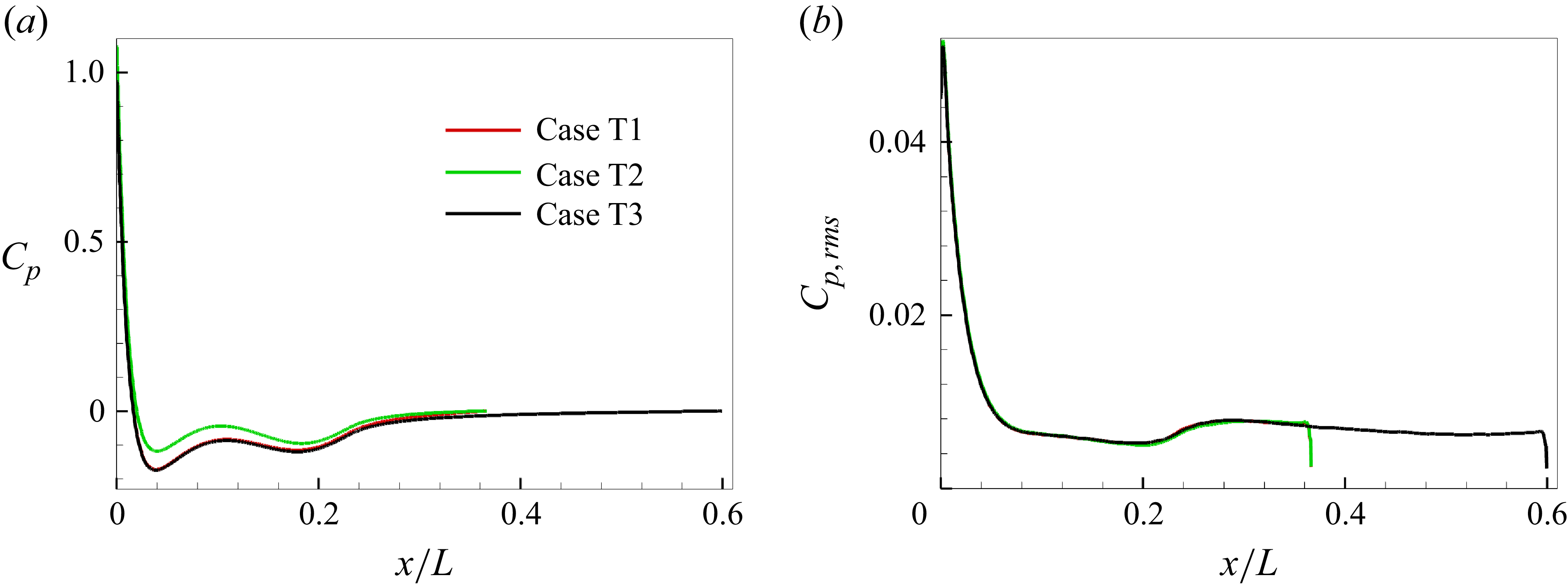
The mean pressure coefficient
 $C_p$
is plotted in figure 13(a), where the previous experiment (Huang & Liu Reference Huang and Liu1994) and numerical simulation (Gross, Kremheller & Fasel Reference Gross, Kremheller and Fasel2011) are included for comparison. The results collapse well and show a good agreement. Note that the experiment of Huang & Liu (Reference Huang and Liu1994) was conducted at
 ${{\mathop {\textit{Re}}\nolimits } _L} = 1.2 \times {10^7}$
, and the Reynolds number of flow simulation in Gross et al. (Reference Gross, Kremheller and Fasel2011) is
 ${{\mathop {\textit{Re}}\nolimits } _L} = 1.4 \times {10^7}$
. The mean pressure coefficient is not affected by the ITI and the Reynolds number. The radius of streamwise curvature
 $R_{\textit{cur}v\textit{e}}$
is also plotted, appearing to roughly correlate with
 $C_p$
, both of which increase in the regions of
 $x/L=0.04{-}0.11$
and
 $x/L=0.18{-}0.23$
, and decrease in the region of
 $x/L=0.11{-}0.18$
. Therefore, the mean pressure coefficient is mainly related to the geometric curvature if there is no trip wire at the wall. Root-mean-square values of WPF are presented in figure 13(b) for cases 0–3. Higher ITI leads to larger pressure fluctuation. In the FPG region, the WPF falls rapidly, and the value becomes nearly zero in case 1. For cases 2 and 3, the changing trend of pressure fluctuation is sensitive to several aspects. Firstly, an important factor is the ITI, as mentioned above. Secondly, the pressure fluctuation changes with the pressure gradient. The adverse pressure gradient causes the fluctuation to increase along the bow. In other words, the pressure fluctuation is affected by the geometric curvature of the bow. Finally, approaching to turbulent equilibrium state will also affect the distribution of the pressure fluctuations. In the rear position of the WPG region, the flow is close to a fully developed turbulent state, resulting in collapse of the curves for cases 2 and 3.
Mean value (a) and r.m.s. (b) of pressure coefficient over the bow surface. The dashed red line represents the radius of streamwise curvature of the bow.

Figure 14 shows the spectra of WPF for different inflow turbulence intensities and different streamwise locations. Three scaling schemes are applied to characterise the spectra to show the differences between the FPG and WPG regions. Note that, for case 1, turbulence in the boundary layer occurs after
 ${x / L} = 0.37$
, and thus the WPF signals in the WPG region are selected at the turbulence generation region, different from cases 2 and 3. The scaling methods of WPF spectra with outer/inner variables have been used in previous studies, such as the pressure spectrum scaling in turbulent flow over a flat plate (Kim Reference Kim1989; Farabee & Casarella Reference Farabee and Casarella1991; Hu et al. Reference Hu, Morfey and Sandham2006), a rough wall (Blake Reference Blake2017), an axisymmetric body (Hong et al. Reference Hong, Shin, Jeon and Kim2008; Hong Reference Hong2015) and other curved walls (Goody & Simpson Reference Goody and Simpson2000; Lee & Sung Reference Lee and Sung2001). Note that the outer-layer variable scaling scheme 2 in figure 14(c,d) shows some difference from the previous studies, due to the influence of ITI in the present study. As shown in figure 14(a,b), higher turbulence level leads to larger pressure fluctuation, causing the upward shift of spectra from case 1 to case 3. In the FPG region, the pressure spectra shift downward along the arc direction due to the suppression effect of the FPG. In the WPG region, turbulence arises, causing the growth of amplitude of the pressure spectra, especially in the high-frequency region.
In the high-frequency region, the scaling law
 ${\varPhi _{pp}} ( \omega ) \sim {\omega ^{ - 5}}$
is found in figure 14, which is the typical characteristic of ZPGTBL (Goody & Simpson Reference Goody and Simpson2000; Aupoix Reference Aupoix2015). In the FPG region, slight offset to the law is recognised owing to the strong pressure gradient. Since small-scale turbulence structures do not appear in the FPG region, as seen in figure 8, it is reasonable to scale the pressure spectra by the outer-layer variable scheme 1 in figure 14(a) (Hong et al. Reference Hong, Shin, Jeon and Kim2008). However, the collapse of spectra for cases 1–3 at different positions is not observed with this scaling scheme. Considering that both different inflow turbulent intensities and continuously changing the pressure gradient along the bow lead to variation of the pressure fluctuation, it is better to introduce the r.m.s. of WPF as the characteristic quantity (scheme 2), as shown in figure 14(c). This scaling scheme results in a more satisfactory collapse of the pressure spectra in the FPG region. In the WPG region, the low-frequency wall pressure spectra are scaled fairly well by the outer-layer variable schemes 1 and 2, although there is a considerable discrepancy for the high-frequency spectra. According to the previous experimental and numerical studies (Farabee & Casarella Reference Farabee and Casarella1991; Lee, Blake & Farabee Reference Lee, Blake and Farabee2005), the inner-layer variable is more appropriate to scale the spectra in the high-frequency region. Due to the small-scale structures, it is helpful to fit all the spectra in the WPG region for cases 1–3 by introducing the inner-layer variable, as seen in figure 14(f).
The WPF spectra over the bow surface scaled by different variables in (a,c,e) the FPG region (solid line:
 ${s / L} = 0.006$
, dash line:
 ${s / L} = 0.01$
, dash dot line:
 ${s / L} = 0.03$
) and (b,d,f) the WPG region (solid line:
 ${s / L} = 0.09$
for case 2 and 3,
 ${s / L} = 0.39$
for case 1; dash line:
 ${s / L} = 0.21$
for case 2 and 3,
 ${s / L} = 0.50$
for case 1; dash dot line:
 ${s / L} = 0.32$
for case 2 and 3,
 ${s / L} = 0.62$
for case 1). Different scaling schemes are applied: (a,b) the outer-layer variable scaling scheme 1, represented by
 ${{\varPhi _{pp}}} / {( {{\delta _{99}}{\rho ^2}{U^3}})}$
versus
 ${\omega {\delta _{99}}} / U$
; (c,d) the outer-layer variable scaling scheme 2, represented by
 ${{\varPhi _{pp}}U} / {( {{\delta _{99}}p\prime _{\textit{rms}}^2} )}$
versus
 ${\omega {\delta _{99}}} / U$
; (e, f) the inner-layer variable scaling, represented by
 ${{\varPhi _{pp}}} / {( {\nu {\rho ^2}u_\tau ^2})}$
versus
 ${\omega \nu } / {u_\tau ^2}$
, where
 $U$
is the mean tangential velocity at the edge of the boundary layer and
 $p{'_{\textit{rms}}}$
is the r.m.s. of WPF.

The spatial distributions of WPF spectra in cases 1 and 2 are presented in figures 15 and 16, respectively. Moreover, the spectra averaged along the circumferential direction are also presented in figure 17. For case 1, which has low ITI (figures 15 and 17
a), the WPF spectrum drops significantly in the FPG region at low frequency (St = 2.3). As the frequency becomes higher (St
 $\gt$
29.6), the WPF spectrum shows the same variation trend as the streamwise curvature radius in figure 13(a). At around x/L = 0.3, a peak of the WPF spectrum is observed at the low-frequency (St
 $\lt$
29.6) area and a valley exists as the frequency becomes higher (St
 $\gt$
29.6), which shows that the natural transition occurs in this region.
The WPF spectra over the bow surface at different frequencies for case 1. The non-dimensional frequency is denoted by the Strouhal number
 $St = {{fL} / U_\infty }$
, and the spectrum
 $\varPhi _{pp}$
is scaled by
 ${p\prime _{\textit{rms}}^2L} / {{U_\infty }}$
.

The WPF spectra over the bow surface at different frequencies for case 2. The frequency and spectrum are scaled by the same variables as in figure 15.

Variations of the WPF spectra along the streamwise direction at different frequencies for (a) case 1 and (b) case 2, which are obtained by averaging over the circumferential direction.

For case 2 (figures 16 and 17
b), the WPF spectra show a similarly changing trend in the FPG region. Owing to the turbulence generation in the WPG region, both the body shape and the ITI act together in the mid- and high-frequency regions (St = 18.2–293.7). The WPF spectrum is larger at the straight section (x/L
 $\gt$
0.23) in the mid-frequency region (St = 18.2–29.6), where the turbulence energy is higher. By comparing the variations of the WPF spectra in figure 17(b) and the radius of streamwise curvature of the bow in figure 13(a), when the frequency is much higher (St
 $\gt$
473.5), there is a strong peak caused by the body shape of the bow.
5. Skin friction
Instantaneous distributions of the skin friction fluctuation over the bow surface in cases 1–3 are presented in figure 18. The skin friction coefficient
 $C_f$
is defined as
 ${C_f} = {{{\tau _w}} / { ( {0.5\rho U_\infty ^2} )}}$
, where
 $\tau _w$
is the wall shear stress at the bow surface. The turbulence intensity in case 1 is relatively low, leading to the late generation of turbulence, and a turbulent spot during the transition process is observed, similar to that in Wu (Reference Wu2023). For the situation with higher inflow turbulence intensities in cases 2 and 3, the streaky structures arise at the front of the WPG region, showing evidence of turbulence generation. The length scale of velocity fluctuation in the FPG region is much larger than that in the WPG region, due to the impact of incoming flow.
Contours of skin friction fluctuation over the bow surface in different cases: (a) case 1; (b) case 2; (c) case 3. Supplementary movie 2 is available online.

The mean skin friction coefficient
 $C_{\!f}$
along the bow surface is presented in figure 19(a). Different from the pressure coefficient,
 $C_{\!f}$
is sensitive to the Reynolds number and the ITI, and no self-similarity can be observed in any of the cases. In the WPG region, higher turbulence intensity results in larger skin friction. The differences between case 0 and the other cases are
 ${C_{\!f,0}} = {C_{\!f,Casei}} - {C_{f,Case{\textrm {0}}}}$
, where i = 1, 2, 3, are given in figure 19(c). For case 1, the position of turbulence generation is approximately at
 ${x / L} = 0.37$
. After that, turbulence develops and
 $C_{f,0}$
grows continuously. For cases 2 and 3, in the FPG region, there exists very slight discrepancy with case 0, and thus
 $C_{f,0}$
is almost zero. Subsequently, thanks to the small adverse pressure gradient at the front part of the WPG region, turbulence arises immediately, and
 $C_{f,0}$
grows rapidly. At the straight section, the skin friction coefficients in cases 2 and 3 collapse as the turbulence equilibrium state is reached. Root-mean-square values of skin friction fluctuation
 $C^{\prime }_{f,\textit{rms}}$
are plotted in figure 19(b). It is seen that the higher the ITI, the larger the skin friction fluctuation along the bow surface. The skin friction fluctuation along the whole bow surface is zero in case 0. For case 1,
 $C^{\prime }_{f,\textit{rms}}$
decays continuously until the growth of turbulence fluctuation. For cases 2 and 3,
 $C^{\prime }_{f,\textit{rms}}$
decreases over the front of the bow. In the region with small adverse pressure gradient, the active disturbance leads to turbulence generation rapidly. At the straight section of the bow, the skin friction fluctuation in cases 2 and 3 is almost the same.
Mean value (a), r.m.s. (b) and net mean value (c) of skin friction coefficient over the bow surface.

Furthermore, based on the dynamic decomposition of
 $C_{\!f}$
in the curvilinear coordinates (
 $s,n,\theta$
), as dictated in (2.9), the generation mechanism of the skin friction can be clarified. According to our calculation of (2.9) by using the flow field data, the results show that the terms related to the geometric parameters
 $K_{\textit{ij}}$
are negligible, as well as
 $C_{\nu 2}$
and
 $C_{D2}$
, and that
 ${{\nabla} ^2}{U_s} \approx {{{\partial ^2}{U_s}} / {\partial {n^2}}}$
. Therefore, (2.9) can be simplified as
 \begin{equation} \begin{array}{l} {C_{\!f}} \approx \underbrace {\frac {2}{{{\textit{Re}}}}{{\left . {{U_s}} \right |}_{{\delta _{99}}}}\beta }_{{C_\nu }}\underbrace { - 2\int _0^1 {\frac {r}{{{{\left . r \right |}_0}}}\overline {{{u'}_{\!s}}{{u'}_{\!n}}} {\rm d}n} }_{{C_R}}\underbrace { - 2\int _0^1 {\left ( {1 - n} \right )\frac {1}{h_s}\frac {{\partial \overline {{{u'}_{\!s}}{{u'}_{\!s}}} }}{{\partial s}}{\rm d}n} }_{{C_D}}\\ \underbrace { - 2\int _0^1 {\left ( {1 - n} \right )\left ( {{U_s}\frac {1}{h_s}\frac {{\partial {U_s}}}{{\partial s}} + {U_n}\frac {{\partial {U_s}}}{{\partial n}}} \right ){\rm d}n} }_{{C_{C1}}}\\ \underbrace { - 2\left ( {\beta - 1} \right )\int _0^1 {\big( {1 - {n^2}} \big)\left ( {{U_s}\frac {1}{h_s}\frac {{\partial {U_s}}}{{\partial s}} + {U_n}\frac {{\partial {U_s}}}{{\partial n}}} \right ){\rm d}n} }_{{C_{C2}}}\\ \underbrace { - 2\int _0^1 {\left ( {1 - n} \right )\frac {1}{h_s}\frac {{\partial P}}{{\partial s}}{\rm d}n} }_{{C_{P1}}}\underbrace { - 2\left ( {\beta - 1} \right )\int _0^1 {\big( {1 - {n^2}} \big)\frac {1}{h_s}\frac {{\partial P}}{{\partial s}}{\rm d}n} }_{{C_{P2}}}. \end{array} \end{equation}
Note that the geometric effect is not explicitly reflected in the above equation. Instead, indirect influences of geometric curvature play a role by altering the mean flow field and modulating the turbulence development along the bow surface, which subsequently impacts the terms of (5.1).
Dynamic decomposition of the skin friction coefficient: (a) comparison with the value calculated by definition; (b–d) contribution ratios of different terms.

The skin friction coefficient
 $C_{f,d}$
calculated by (5.1) is compared with that obtained directly by its definition
 ${C_{\!f}} = {{ ( {{{\nu \partial {U_s}} / {\partial n}}} )} / { ( {0.5U_\infty ^2} )}}$
in figure 20(a), which shows a good agreement. Ratios of the terms in (5.1) to local mean skin friction coefficient are shown in figure 20(b–d). The variations of all the terms are sensitive to the streamwise curvature of the bow. In other words, the bluff body induces variations of the mean velocity and pressure gradient, which then contribute to the other terms. As a consequence of the flow acceleration in the FPG region, the mean tangential velocity of external flow
 $\left . {{U_s}} \right |_{{\delta _{99}}}$
grows rapidly along the arc direction from the stagnation point. Despite the decrease of the Reynolds number
 ${\mathop {\textit{Re}}\nolimits } = {{{U_\infty }{\delta _{99}}} / \nu }$
, the fast increase of
 $\left . {{U_s}} \right |_{{\delta _{99}}}$
causes the sustainable growth of
 $C_\nu$
, which cannot be ignored in the FPG region and the front part of the WPG region. The Reynolds shear stress term
 $C_R$
is nearly zero in the front part of the bow owing to the turbulence suppression effect. In the WPG region, turbulence grows gradually, and the ratio of
 $C_R$
keeps the value of approximately 40 % as the turbulence reaches its equilibrium state. Here,
 $C_D$
is relatively small over the whole bow surface, and is zero in the ZPGTBL flow. Its two growth zones correspond to the area of increasing curvature of the bow, which is also the region where the adverse pressure gradient exists (seen in figure 13
a). This reflects the influence of geometric shape on the development of Reynolds stress. The values of
 $C_{C1}$
,
 $C_{C2}$
,
 $C_{P1}$
and
 $C_{P2}$
also show a similarly changing trend. In figure 20(c), it can be seen that the mean convection and pressure-gradient terms,
 $C_{C1}$
and
 $C_{P1}$
, contribute to the local skin friction the most overall. The most obvious inflection point of
 $C_{C1}$
and
 $C_{P1}$
appears at the junction of the curved wall and the straight sections, at approximately
 ${x / L} = 0.23$
. Note that
 $C_{P1}$
reflects the influence of not only the pressure gradient, but also the boundary layer thickness. Therefore, considering their combined influences, the maximum value appears at
 ${x / L} = 0.23$
, rather than at the stagnation point intuitively, where the largest pressure gradient exists. In figure 20(d), it can be considered that
 ${C_{C2}} \approx 0.1{C_{C1}}$
and
 ${C_{P2}} \approx 0.1{C_{P1}}$
, owing to the fact that the boundary layer thickness is an order of magnitude smaller than the local radius of the bow. Nonetheless, the contribution of
 $C_{C2}$
and
 $C_{P2}$
to the skin friction cannot be ignored. It should be mentioned that the mean-pressure-gradient terms
 $C_{P1}$
and
 $C_{P2}$
also reflect the effect of the streamwise curvature, since the radius of streamwise curvature
 $R_{\textit{cur}v\textit{e}}$
plotted in figure 13(a) appears to roughly correlate with the mean pressure coefficient
 $C_{p}$
.
6. Budget analysis
For the budget analysis in the curvilinear coordinate system, the Reynolds stress transport equations are given in (2.11), including the production term
 $P$
, the turbulent transport term
 $DT$
, the pressure transport term
 $DP$
, the viscous diffusion term
 $D\nu$
, the pressure-strain or redistribution term
 $\varPhi$
, the dissipation term
 $\varepsilon$
and the geometric term
 $R_{\textit{geo}}$
as given by (2.12). In the curvilinear coordinate (
 $s,n,\theta$
) system, two streamwise locations are selected to present the budget analysis for case 2. One is at
 ${s / L} = 0.01$
in the FPG region, where the friction Reynolds number is
 $\textit{Re}_\tau = 20$
, and the other is at
 ${s / L} = 0.32$
in the WPG region with
 $\textit{Re}_\tau = 300$
. The budget terms for the tangential, normal and spanwise Reynolds normal stresses and Reynolds shear stress are shown in figure 21. Note that every term in figure 21 is the combination of geometric and non-geometric terms. In the rear position of the WPG region, the budget relationships for the different components are quite similar to those in a turbulent channel flow (Lee & Moser Reference Lee and Moser2018). For the areas beyond the boundary layer (
 ${n^ + } \gt 300$
), the budget terms fall to zero. On the contrary, the budget relationships in the FGP region exist not only within the boundary layer. The turbulent transport term, viscous diffusion term and dissipation term drop to zero beyond the boundary layer, while the other non-zero terms in (2.11) extend outward in the normal direction, much further away from the wall than the boundary layer thickness.
Budget terms in case 2: (a,c,e,g)
 ${s/ L} = 0.01$
; (b,d,f,h)
 ${s/ L} = 0.32$
. (a,b) Tangential, (c,d) normal and (e,f) spanwise components of Reynolds normal stresses; (g,h) Reynolds shear stress. The dash-dotted black lines represent locations of the outer edge of the boundary layer.

Budget terms for Reynolds shear stress at
 ${s / L} = 0.01$
in case 2, with summation of
 $DP$
and
 $\varPhi$
.

Key budget terms at different streamwise positions for case 2: (a,c,e,g) the production term; (b,d,f,h) the redistribution term. (a,b) Tangential, (c,d) normal and (e,f) spanwise components of Reynolds normal stresses; (g,h) Reynolds shear stress.

To clarify the differences between the FPG and WPG regions more clearly, the budget relationships in the FPG region are presented in more detail. As shown in figure 21(a) for
 $\overline {{{u'}_s}{{u'}_s}}$
, the pressure-strain term plays a major role in the budget. A negative production term is observed, which reflects the suppression effect on turbulence generation in this region. For the normal component (figure 21
c), only the influences of pressure fluctuation,
 $DP$
, and
 $\varPhi$
dominate within the boundary layer, while outside of the boundary layer a positive production term becomes the main term, which is zero throughout the boundary layer in turbulent channel flow. For the spanwise component (figure 21
e), a non-zero production term is balanced with
 $\varPhi$
, especially outside of the boundary layer. For the Reynolds shear stress (figure 21
g), due to the large pressure fluctuation caused by the disturbance from the incoming flow,
 $DP$
and
 $\varPhi$
are dominant across the entire region. Since the values of
 $DP$
and
 $\varPhi$
are nearly opposite, to show the distribution of the other terms, they are combined and are compared with the other terms in figure 22. It is seen that their summation balances with the production term in the FPG region. Similar to figure 21(a,e), the production term is negative, indicating the suppression effect on turbulence generation.
Since the production and redistribution terms are the key terms in the budget of the Reynolds stresses, they are plotted at different streamwise positions for case 2 in figure 23. Due to the suppression effect of FPG, the key terms drop rapidly in the FPG region. In the WPG region, the turbulence develops in the boundary layer. The same changing trends are observed as those of velocity fluctuations and Reynolds shear stress, as shown in figure 11.
Now the geometric effects are discussed according to (2.12). Due to the fact that the large streamwise curvature exists in the FPG region, the geometric effects are investigated only in this region. The geometric effects of the turbulent transport term and viscous term are small, compared with that of the production term. Therefore, only the geometric and non-geometric parts of the production term are considered, which are expressed as
 \begin{align} \begin{array}{l} \textit{For}\,\overline {{{u'}_s}{{u'}_s}} ,\left \{ \begin{array}{l} {P_{\textit{non}} - {\textit{geo}}} = - 2\overline {{{u'}_s}{{u'}_s}} \dfrac {1}{{{h_s}}}\dfrac {{\partial {U_s}}}{{\partial s}} - 2\overline {{{u'}_s}{{u'}_n}} \dfrac {{\partial {U_s}}}{{\partial n}},\\{P_{\textit{geo}}} = - 2\overline {{{u'}_s}{{u'}_s}} {K_{\textit{sn}}}{U_n}. \end{array} \right .\\[16pt]\textit{For}\,\overline {{{u'}_n}{{u'}_n}} ,\left \{ \begin{array}{l} {P_{\textit{non}} - {\textit{geo}}} = - 2\overline {{{u'}_s}{{u'}_n}} \dfrac {1}{{{h_s}}}\dfrac {{\partial {U_n}}}{{\partial s}} - 2\overline {{{u'}_n}{{u'}_n}} \dfrac {{\partial {U_n}}}{{\partial n}},\\{P_{\textit{geo}}} = 2\overline {{{u'}_s}{{u'}_n}} {K_{\textit{sn}}}{U_s}. \end{array} \right .\\[16pt]\textit{For}\,\overline {{{u'}_\theta }{{u'}_\theta }} ,\left \{ \begin{array}{l} {P_{\textit{non}} - {\textit{geo}}} = 0,\\{P_{\textit{geo}}} = - 2\overline {{{u'}_\theta }{{u'}_\theta }} \left ( {{K_{\theta s}}{U_s} + {K_{\theta n}}{U_n}} \right )\! .\end{array} \right .\\[12pt]\textit{For} - \overline {{{u'}_s}{{u'}_n}} ,\left \{ \begin{array}{l} {P_{\textit{non}} - {\textit{geo}}} = 2\overline {{{u'}_n}{{u'}_n}} \dfrac {{\partial {U_s}}}{{\partial n}} + \overline {{{u'}_s}{{u'}_s}} \dfrac {1}{{{h_s}}}\dfrac {{\partial {U_n}}}{{\partial s}} + \overline {{{u'}_s}{{u'}_n}} \left ( {\dfrac {1}{{{h_s}}}\dfrac {{\partial {U_s}}}{{\partial s}} + \dfrac {{\partial {U_n}}}{{\partial n}}} \right )\!,\\{P_{\textit{geo}}} = - \overline {{{u'}_s}{{u'}_s}} {K_{\textit{sn}}}{U_s} + \overline {{{u'}_s}{{u'}_n}} {K_{\textit{sn}}}{U_n}, \end{array} \right . \end{array} \end{align}
and are shown in figure 24 for different components of the Reynolds stresses. In the FPG region, the Reynolds shear stress is much smaller than the Reynolds normal stresses, and the terms with
 $- \overline {{{u'}_s}{{u'}_n}}$
in (6.1) can be ignored. Thus, as seen in figure 24, for the production term of
 $\overline {{{u'}_n}{{u'}_n}}$
, the non-geometric term is dominant and the geometric effect is negligible. Flow acceleration in the FPG region leads to significant
 ${\partial {U_s}} / {\partial s}$
, explaining the fact that the non-geometric term plays a major role for the production term of
 $\overline {{{u'}_s}{{u'}_s}}$
. For the production term of
 $\overline {{{u'}_\theta }{{u'}_\theta }}$
, the non-geometric term is zero, and the geometric effect contributes to the whole production term. For the production term of
 $- \overline {{{u'}_s}{{u'}_n}}$
, the geometric and non-geometric effects have similar magnitudes, as seen in figure 24(d).
Geometric (solid lines) and non-geometric (dashed lines) parts of the production term for case 2: (a) tangential, (b) normal and (c) spanwise components of Reynolds normal stresses; (d) Reynolds shear stress.

According to the above budget analysis, the paths of energy transfer in the FPG region are summarised in figure 25. The FPG suppresses the development of turbulence, and causes the decreases of absolute values of budget terms. As a result, the intensities of Reynolds normal stresses and Reynolds shear stress are decreased rapidly along the streamwise direction. Here,
 $P$
and
 $\varPhi$
play the dominant roles in the budget of Reynolds normal stresses outside of the boundary layer, while only
 $DP$
and
 $\varPhi$
are dominant for the Reynolds shear stress. The geometric effects are reflected in the production term, especially for the spanwise Reynolds normal stress and Reynolds shear stress.
Schematic of paths of energy transfer in the FPG region. Red arrows denote the changing of absolute values; black arrows denote the directions of paths of energy transfer; green arrows denote the dominant budget relationships.

7. Conclusions
Under the condition of turbulent inflow, simulation of flow over the bow of SUBOFF was performed using wall-resolved LES at a Reynolds number of
 ${{\mathop {{Re}}\nolimits } _L} = 1.1 \times {10^6}$
. Instead of applying trip wires as in the previous studies, where the flow over the bow region with large streamwise curvature was not of concern, cases with varying ITI were simulated in the present study to investigate the characteristics of the curved boundary layer over the bow. The results showed that the ITI has a significant impact on the flow development, and larger intensity causes turbulence to occur earlier and then leads to larger skin friction before attaining the turbulent equilibrium state. However, the location of transition cannot move upstream further in the FPG region as the ITI increases continuously, due to the strong FPG caused by large curvature. The phenomena in the FPG region differ from those of a flat plate. The FPG effectively suppresses turbulence generation, causing velocity and pressure fluctuations in the boundary layer to decrease quickly along the bow profile and concentrate mainly in the low-frequency range. The consistently maintained laminar state in the FPG region causes that the boundary layer statistics, such as the nominal thickness of boundary layer, momentum thickness and frictional Reynolds number and tangential velocity profiles, vary minimally across different ITI cases. Wall pressure has received widespread attention, and the present study showed that both the bow shape and ITI play a crucial role on its evolution. The bow shape forms the unique mean pressure distribution, which is not affected by ITI. Subsequently, the generated strong FPG near the stagnation point leads to the rapid declination of WPF along the bow profile. In the FPG region, the scales of WPF are much larger than those in the WPG region, resulting in wall pressure spectra being well scaled by the outer variables related to the intensity of WPF. In the high-frequency region, the WPF spectra show the same variation trend as the streamwise curvature of the bow, so a noticeable spectral peak appears at the mid part of the bow. In the FPG region, WPF is primarily generated by inflow disturbances, and thus larger ITI leads to larger pressure fluctuation. Conversely, in the WPG region, once a fully developed turbulent state is attained, WPF is not affected by ITI, so the WPF spectra are scaled well by the inner variables. Furthermore, dynamic decomposition of the skin friction showed that, due to the unique body shape of the bow, the mean convection and streamwise pressure gradient contribute the most to the local skin friction. This explains why the changing trend of skin friction is similar to that of the mean pressure. Budget analysis on the Reynolds stress transport equations in the curvilinear system indicated that the negative production terms for
 $\overline {{{u'}_{\!\theta} }{{u'}_{\!\theta} }}$
and
 $ - \overline {{{u'}_s}{{u'}_n}}$
are formed by the bow curvature, causing them to decrease rapidly in the FPG region, while the terms related to pressure fluctuation are dominant for Reynolds shear stress.
Supplementary movies
Supplementary movies are available at https://doi.org/10.1017/jfm.2025.10820.
Acknowledgements
The authors are thankful to the anonymous reviewers for their valuable comments and suggestions.
Funding
This work was supported by the National Natural Science Foundation of China under grant nos. 12425206, 12272206, 92252204 and 12388101.
Declaration of interests
The authors report no conflict of interest.
Appendix A. Validation case I: flow over the SUBOFF model with trips
The present algorithm is validated by simulation of the flow around the axisymmetric SUBOFF bow at zero angle of pitch and yaw. The Reynolds number is fixed at
 $\textit{Re}_L = {{{U_\infty }L} / \nu } = 1.1 \times {10^6}$
. The details for the computation settings are shown in figure 26. By applying a steady wall-normal velocity at the same location (x/R = 1.5) as that in Morse & Mahesh (Reference Morse and Mahesh2021), the flow is tripped so that turbulence arises quickly. To reduce the cost of computation, only a 1/25 circumferential segment of the SUBOFF bow is used here. Constant velocity is given along the inflow surface, and a no-slip condition is applied at the wall. Constant-pressure condition is used at the outlet. Periodic boundary condition is used for the two spanwise planes. The nominal grid sizes at the wall are set to
 $\Delta {s^ + } \approx 12$
,
 $\Delta n_w^ + \lt 1$
and
 $r\Delta {\theta ^ + } \approx 6$
, leading to a grid number of approximately 127 million.
Details of computation settings for simulation of the flow around the SUBOFF bow.

The mean pressure coefficient
 $C_p$
on the bow surface is compared with the previous numerical and experimental data in figure 27(a). Since a non-zero wall-normal velocity is applied at the position x/R = 1.5 (x/L = 0.087), a notable pressure interruption is observed here. The present
 $C_p$
agrees well with the reference data overall, despite small differences after blowing owing to the different blowing velocity. The present skin friction coefficient
 $C_{\!f}$
is compared with the previous data in figure 27(b). After transition, the present
 $C_{\!f}$
compares well with the reference data. Also, the theoretical
 $C_{\!f}$
for a flat-plate ZPGTBL (Schlichting & Kestin Reference Schlichting and Kestin1961) is shown here for comparison, which is expressed as
 \begin{equation} {C_{\!f}} = 0.0576{Re}_s^{ - 0.2} = 0.0576{\left [ {\frac {{{U_\infty }\left ( {s - {s_0}} \right )}}{\nu }} \right ]^{ - 0.2}}, \end{equation}
where
 $s_0$
is the origin, chosen at the location of wall blowing. Since the longitudinal curvature is relatively small, and the thickness of TBL is an order of magnitude smaller than the local radius of the bow, the theoretical
 $C_{\!f}$
is suitable to describe the development of the skin friction coefficient in the region after the trip wire.
Mean pressure (a) and friction (b) coefficients over the bow surface.

Figure 28 shows the evolution of the bow boundary layer in terms of the following parameters: the nominal thickness
 $\delta _{99}$
, the shape factor
 $H$
, the momentum-thickness Reynolds number
 $\textit{Re}_\theta $
and the friction Reynolds number
 $\textit{Re}_\tau $
. Notice that
 $H = {{{\delta ^*}} / \theta }$
, with
 $\delta ^*$
denoting the displacement thickness and
 $\theta$
the momentum thickness,
 $\textit{Re}_\theta = {{{U_\infty }\theta } / \nu }$
,
 $\textit{Re}_\tau = {{{u_\tau }{\delta _{99}}} / \nu }$
. Based on the hypothesis of a −1/7 power or log law for the tangential velocity profile, i.e.
 \begin{align} \frac {{{U_s}}}{{{u_\tau }}} = C{\left ( {\frac {{y{u_\tau }}}{\nu }} \right )^{{1 / 7}}},C = 8.74, \\[-29pt] \nonumber \end{align}
 \begin{align} \left \{ \begin{array}{l} \dfrac {{{U_s}}}{{{u_\tau }}} = \dfrac {1}{\kappa }\ln \dfrac {{y{u_\tau }}}{\nu } + B + \dfrac {{2\prod }}{\kappa }{\sin ^2}\left ( {\dfrac {\pi }{2}\dfrac {y}{\delta }} \right )\\[12pt]\kappa = 0.41,B{\textrm { = 5}}{\textrm {.0, }}\prod = 0.5 \end{array} \right ., \\[9pt] \nonumber \end{align}
two analytical solutions for a flat-plate ZPGTBL are also plotted in figure 28, and show reasonable agreements with the present numerical results of
 $\delta _{99}$
,
 $H$
,
 $\textit{Re}_\theta $
and
 $\textit{Re}_\tau $
. A trip wire with larger blowing velocity is used, and thus a jump of the shape factor occurs in the transitional region.

Furthermore, wall-normal distributions for inner-scaled data at x/D = 5.4 are plotted in figure 29. In table 2, the present
 $\textit{Re}_\tau $
and
 $\textit{Re}_\theta $
at this location are compared with those of the flat-plate TBL and over the SUBOFF bow. There is a negligible streamwise pressure gradient and the nominal thickness of TBL is much smaller than the bow radius at x/D = 5.4, so the velocity and pressure fluctuations collapse well for the present and previous studies. In the tangential velocity profile, the linear and log laws are clearly observed.
The friction Reynolds number and the Reynolds number based on momentum thickness of the present study, compared with the previous studies. Note that the data in Morse & Mahesh (Reference Morse and Mahesh2021) also come from the location at x/D = 5.4.

Profiles of (a) mean tangential velocity, (b) r.m.s. of tangential velocity fluctuation, (c) r.m.s. of normal velocity fluctuation, (d) r.m.s. of spanwise velocity fluctuation, (e) Reynolds shear stress and (f) r.m.s. of pressure fluctuation along the wall-normal direction at x/D = 5.4.

Appendix B. Validation case II: flow transition of the flat-plate boundary layer
To further validate the numerical solver, the flow transition of the flat-plate boundary layer is simulated, as sketched in figure 30. At the inlet, the mean velocity profiles obtained by a 2-D laminar flow simulation are applied, as shown in figure 31. The inlet Reynolds number is
 $\textit{Re}_x=U_\infty x/\nu =2.5\times 10^5$
, where
 $U_\infty$
is the free-stream velocity and
 $\nu$
is the kinematic viscosity, which is the same as that in Kim et al. (Reference Kim, Lim, Kim, Jee, Park and Park2019). The size of computational domain is
 $L_x \times L_y \times L_z = 321 \delta _0 \times 18 \delta _0 \times 8\delta _0$
, where
 $\delta _0$
is the nominal boundary layer thickness at the inlet. No-slip condition is applied at the flat plate and a constant-pressure condition is used at the outlet. Periodic boundary condition is adopted in the spanwise direction. At the upper boundary, a zero normal-gradient condition is employed for both the velocity and pressure.
Schematic of the computational settings for flow over a flat plate.

Mean velocity profiles adopted at the inlet.

To induce flow transition, velocity disturbance is introduced at the inlet. The disturbance can be decomposed into a fast-varying oscillatory-wave part and a slow-varying part, which is expressed as follows:
 \begin{equation} {{u}^\prime_{\!i}}( {y,z,t}) = \sum \limits _{m = - {N_m}}^{{N_m}} {\sum \limits _{n = - {N_n}}^{{N_n}} {{A_{( {m,n})}}( {y,z,t})\exp \left ( {i{\varphi _{\left ( {m,n} \right )}} + in\chi z - im\omega t} \right ),i = 1,2,3} } . \end{equation}
For validation purposes, the parameters are selected to be consistent with those of Kim et al. (Reference Kim, Lim, Kim, Jee, Park and Park2019). The fundamental wave of
 $F = 2\pi f\nu / U_\infty ^2 = 1.24 \times 10^{ - 4}$
for mode
 $(m,n)=(2,0)$
and the subharmonic wave for mode
 $(m,n)=(1,1)$
are introduced. The spanwise wavenumber of the subharmonic mode is
 $\chi = 2\pi \delta _0 / L_z=0.6506$
, and the angular frequency of the fundamental wave is
 $\omega = 2\pi f\delta _0 / U_\infty =0.2477$
. Here,
 $A_{(2,0)\textit{max}}=5.2\times 10^{-3}$
and
 $A_{(1,1)\textit{max}}=8.5\times 10^{-5}$
are selected. The shapes of these two disturbance modes are displayed in figure 32. It is seen that the streamwise component is dominant for the two modes.
Amplitude and phase profiles of the 2-D fundamental and subharmonic oblique waves at
 $\textit{Re} = 2.5\times 10^5$
: (a) amplitude of the 2-D T–S wave; (b) phase of the 2-D T–S wave; (c) amplitude of the subharmonic wave; (d) phase of the subharmonic wave.

The grid number is set to
 $N_x \times N_y \times N_z=3072 \times 128 \times 128$
, resulting in the grid resolution of
 $\Delta x_{\textit{max}}^+=12.7$
,
 $\Delta y_{w,\textit{max}}^+=0.44$
and
 $\Delta z_{\textit{max}}^+=7.4$
. The first wall-normal grid is set to
 $\Delta y_1=0.0036\delta _0$
, and the number of wall-normal grid points within the boundary layer at the inlet is 54. The computational time step is set to
 $\Delta t \times U_\infty /\delta _0=0.077$
and the maximum Courant-Friedrichs-Lewy (CFL) number is less than 2. Flow statistics are computed over a 4.2 flow-through time after reaching the statistically steady state.
Figure 33 shows the development of instantaneous vortical structures of the flat-plate boundary layer. The 2-D wave is dominant near the inlet. The instability of spanwise mode gradually arises, leading to the formation of
 $\varLambda$
-shape vortical structures at around
 $\textit{Re}_x=4.5 \times 10^5-5 \times 10^5$
. Then the
 $\varLambda$
-shape structures turns into hairpin vortices, and flow transition completes. Such transition process is often called the H-type transition (Kachanov Reference Kachanov1994).
Instantaneous vortical structures coloured by the streamwise velocity
 $u_x$
: (a) top view; (b) 3-D view.

Figure 34 shows the streamwise evolution of the skin friction coefficient, from which the transition process is clearly observed. The present result is compared with the DNS data (Sayadi, Hamman & Moin Reference Sayadi, Hamman and Moin2013; Lozano-Durán et al. Reference Lozano-Durán, Hack and Moin2018) and the LES data (Kim et al. Reference Kim, Lim, Kim, Jee, Park and Park2019). The theoretical laminar and turbulent solutions are also included for comparison, which are expressed as
 $C_{\!f}=0.664\sqrt {{Re}_x}$
and
 $C_{\!f}=0.455/\textrm {ln}^2(0.06\textit{Re}_{x})$
(White& Majdalani Reference White and Majdalani2006), respectively. Good agreements can be found in figure 34, demonstrating the accuracy of the present numerical solver in simulating the boundary layer flow transition.
Streamwise evolution of the skin friction coefficient of boundary layer over a flat plat.

Appendix C. Verification of the inlet/outlet computational settings
To verify the feasibility of the non-uniform inlet condition shown in figure 1 and explore the influence of the constant-pressure outlet condition, additional simulations are performed as listed in table 3. Cases with non-uniform (T1) and uniform (T2) inlet velocities are tested to show the influence of inflow condition, and cases T1 and T3 with different domain lengths are tested to show the influence of the outlet boundary condition. Along the inflow surface, with a turbulence intensity of 20 % for all cases, the turbulence intensity at the
 $x=0$
plane is 4.6 %. Moreover, the distance between inflow surface and bow surface is
 $3.6R$
, which is the same as that in table 1.
Computational parameters for different cases for verification.

Streamwise evolution of turbulence intensity at
 $r/R=1.1$
.

For all the three cases, the Reynolds number is
 $\textit{Re}_L=1.1\times 10^6$
. To reduce the computational cost, the grid sizes at the bow surface satisfy
 $\Delta {s^ + } \lt 36$
and
 $r\Delta {\theta ^ + } \lt 32$
, and the first wall-normal grid resolution satisfies
 $\Delta n_w^ + \lt 1$
, resulting in a total of 88 million grids for cases T1 and T2, and 130 million grids for case T3. The computational time step is
 $\Delta t {{{U_\infty }} / L} = 2.1 \times {10^{ - 4}}$
, ensuring that the maximum local CFL number is less than 1. After reaching the statistically steady state, the data over a 6 flow-through-body time are then used to compute the statistics.
Figures 35 and 36 show the streamwise evolution of the turbulence intensity of outer flow and the pressure coefficients along the bow surface, respectively. By comparing the results of cases T1 and T2, it can be seen that the data show a slight but discernible difference (figure 36 a). To avoid excessive dissipation of incoming turbulent fluctuations, the computational domain size should not be set too large. Therefore, the non-uniform velocity inlet condition is more suitable in the present study. In addition, the results are almost the same for cases T1 and T3, except that the r.m.s. of WPF is affected by the outlet condition within a small region very close to the outlet, as shown in figure 36(b).
Streamwise evolution of (a) mean wall pressure coefficient and (b) r.m.s. of its fluctuation over the bow surface.

Appendix D. Governing equations in the axisymmetric bow-profile coordinate system
In a general curvilinear coordinate system, by introducing a covariant unit base vector
 $\boldsymbol{e}_i$
and contracovariant unit base vector
 $\boldsymbol{e}^i$
, the velocity vector is expressed as
 ${\boldsymbol{u}} = {u^i}{{\boldsymbol{e}}_{\boldsymbol{i}}} = {u_i}{{\boldsymbol{e}}^{\boldsymbol{i}}}$
, where
 $u^i$
and
 $u_i$
are contracovariant and covariant components of
 $\boldsymbol{u}$
, respectively. The covariant general metric tensor
 $g_{\textit{ij}}$
can be written as
 \begin{equation} {g_{\textit{ij}}} = {\delta _{\textit{mn}}}\frac {{\partial {x^m}}}{{\partial {\xi ^i}}}\frac {{\partial {x^n}}}{{\partial {\xi ^j}}},{\delta _{\textit{mn}}} = \left \{ \begin{array}{l} 1,{\textrm { i = j}},\\ {\textrm {0, i}} \ne {\textrm {j}} ,\end{array} \right . \end{equation}
where
 $x^m$
and
 $\xi ^i$
are the contravariant components of the Cartesian and general curvilinear coordinates, respectively. The different terms of the N–S equations in a general curvilinear coordinate can be written as follows (Richmond et al. Reference Richmond, Chen and Patel1986):
 \begin{equation} \begin{array}{l} \dfrac {{\partial {\boldsymbol{u}}}}{{\partial t}}:\,\,\,\,\,\,\dfrac {{\partial {u_i}}}{{\partial t}},\\[5pt]{\boldsymbol{u}} \boldsymbol{\cdot }\boldsymbol{\nabla }{\boldsymbol{u}}:\,{u_m}\dfrac {{\partial {u_i}}}{{\partial {\xi _m}}} + {D_{\textit{im}}}{u_m}{u_i} + {\varGamma _{\textit{imn}}}{u_m}{u_n},\\[5pt]- \dfrac {{\boldsymbol{\nabla }p}}{\rho }:\,\,\, - g_{\textit{im}}^c\dfrac {\partial }{{\partial {\xi _m}}}\left ( {\dfrac {p}{\rho }} \right )\!,\\[5pt]\nu \Delta {\boldsymbol{u}}:\,\,\,\,\,\nu \left \{ {{{\nabla} ^2}{u_i} + 2{E_{\textit{im}}}\dfrac {{\partial {u_i}}}{{\partial \xi \left ( m \right )}} + 2{C_{\textit{imn}}}\dfrac {{\partial {u_n}}}{{\partial \xi \left ( m \right )}} + {P_i}{u_i} + {Q_{\textit{in}}}{u_n}} \right \}\\[5pt]\boldsymbol{\nabla }\boldsymbol{\cdot }{\boldsymbol{u}}:\,\,\,\,\,\dfrac {\partial }{{\partial {\xi ^i}}}\left ( {\dfrac {{{g^{{1 / 2}}}{u_i}}}{{g_{\textit{ii}}^{{1 / 2}}}}} \right )\!, \end{array} \end{equation}
where
 \begin{align} {u_i} & = g_{\textit{ii}}^{{1 / 2}}{u^i},\frac {\partial }{{\partial {\xi _m}}} = g_{\textit{mm}}^{{{ - 1} / 2}}\frac {\partial }{{\partial {\xi ^m}}},\nonumber\\[5pt]{D_{\textit{im}}} & = g_{\textit{ii}}^{{1 / 2}}\frac {{\partial g_{\textit{ii}}^{{{ - 1} / 2}}}}{{\partial {\xi _m}}},{\varGamma _{\textit{imn}}} = g_{\textit{ii}}^{{1 / 2}}g_{\textit{mm}}^{{{ - 1} / 2}}g_{\textit{nn}}^{{{ - 1} / 2}}\varGamma _{\textit{mn}}^i,\nonumber\\[5pt]g_{\textit{im}}^c & = g_{\textit{ii}}^{{1 / 2}}g_{\textit{mm}}^{{1 / 2}}{g^{\textit{im}}},{g^{{1 / 2}}} = \left | {{g_{\textit{ij}}}} \right |, \nonumber\\[5pt]{P_i} & = g_{\textit{ii}}^{{1 / 2}}\Delta g_{\textit{ii}}^{{{ - 1} / 2}} , \end{align}
and
 \begin{align}{E_{\textit{im}}} & = g_{\textit{mn}}^c{D_{\textit{in}}},{C_{\textit{imn}}} = g_{ml}^c{\varGamma _{iln}},\nonumber\\{Q_{\textit{in}}} & = \frac {{\partial {C_{\textit{imn}}}}}{{\partial {\xi _m}}} + \left ( {{D_{\textit{im}}} + {D_{nm}} + {D_{\textit{mm}}} + {\varGamma _{llm}}} \right ){C_{\textit{imn}}} + {C_{iml}}{\varGamma _{lmn}},\nonumber\\\varDelta & = {{\nabla} ^2} = g_{\textit{mm}}^{{{ - 1} / 2}}g_{\textit{nn}}^{{{ - 1} / 2}}g_{\textit{mn}}^c\frac {{{\partial ^2}}}{{\partial {\xi ^m}\partial {\xi ^m}}} + {f_m}\frac {\partial }{{\partial {\xi _m}}},{f_m} = - g_{\textit{ij}}^c{\varGamma _{mij}}. \end{align}
The Christoffel symbol is defined as
 \begin{equation} \varGamma _{\textit{jk}}^i = {{{g^{il}}\big ( {{{\partial {g_{lj}}} / {\partial {\xi ^k}}} + {{\partial {g_{kl}}} / {\partial {\xi ^j}}} - {{\partial {g_{\textit{jk}}}} / {\partial {\xi ^l}}}} \big )} / 2}. \end{equation}
Then choose an axisymmetric bow-profile coordinate system (
 $s,n,\theta$
), as described in § 2.1. The covariant general metric tensor
 $g_{\textit{ij}}$
in (D1) can be written as
 \begin{equation} {g_{\textit{ij}}} = \left \{ \begin{array}{l} h_i^2,{\textrm { i = j}},\\ {\textrm {0, i}} \ne {\textrm {j}} ,\end{array} \right . \end{equation}
where
 $h_i$
is the Lame coefficient in the orthogonal coordinate system (Richmond et al. Reference Richmond, Chen and Patel1986). Therefore, (D2) can be simplified as follows:
 \begin{align} & \!\! \frac {{\partial {\boldsymbol{u}}}}{{\partial t}}:\,\,\,\,\,\,\frac {{\partial {u_i}}}{{\partial t}},\nonumber\\& \!\! {\boldsymbol{u}} \boldsymbol{\cdot }\boldsymbol{\nabla }{\boldsymbol{u}}:\,{u_i}\frac {{\partial {u_i}}}{{\partial {\xi _i}}} + {u_{\!j}}\frac {{\partial {u_i}}}{{\partial {\xi _{\!j}}}} + {u_k}\frac {{\partial {u_i}}}{{\partial {\xi _k}}} + {K_{\textit{ij}}}{u_i}{u_{\!j}} - {K_{\textit{ji}}}{u_{\!j}}{u_{\!j}} + {K_{\textit{ik}}}{u_i}{u_k} - {K_{\textit{ki}}}{u_k}{u_k},\nonumber\\& \!\! - \frac {{\boldsymbol{\nabla }p}}{\rho }:\,\,\, - \frac {\partial }{{\partial {\xi _i}}}\left ( {\frac {p}{\rho }} \right )\!,\nonumber\\& \!\! \nu \Delta {\boldsymbol{u}}:\, \nu \!\left \{ {{{\nabla} ^2}{u_i} + 2{K_{\textit{ij}}}\frac {{\partial {u_{\!j}}}}{{\partial {\xi _i}}} + 2{K_{\textit{ik}}}\frac {{\partial {u_k}}}{{\partial {\xi _i}}} - 2{K_{\textit{ji}}}\frac {{\partial {u_{\!j}}}}{{\partial {\xi _{\!j}}}} - 2{K_{\textit{ki}}}\frac {{\partial {u_k}}}{{\partial {\xi _k}}} + {\alpha _{\textit{ii}}}{u_i} + {\alpha _{\textit{ij}}}{u_{\!j}} + {\alpha _{\textit{ik}}}{u_k}} \! \right \}\!,\nonumber\\& \!\! \boldsymbol{\nabla }\boldsymbol{\cdot }{\boldsymbol{u}}:\,\,\,\,\,\frac {{\partial {u_i}}}{{\partial {\xi _i}}} + \frac {{\partial {u_{\!j}}}}{{\partial {\xi _{\!j}}}} + \frac {{\partial {u_k}}}{{\partial {\xi _k}}} + \left ( {{K_{\textit{ji}}} + {K_{\textit{ki}}}} \right ){u_i} + \left ( {{K_{\textit{ij}}} + {K_{\textit{kj}}}} \right ){u_{\!j}} + \left ( {{K_{\textit{ik}}} + {K_{\textit{jk}}}} \right ){u_k}. \end{align}
The expressions of
 $K_{\textit{ij}}$
and
 $\alpha _{\textit{ij}}$
are given in (2.8).
Note that, for flow over the axisymmetric bow in the (
 $s,n,\theta$
) coordinates,
 ${K_{s\theta }} = {K_{ns}} = {K_{\textit{nn}}} = {K_{n\theta }} = {K_{\theta \theta }} = 0$
. In figure 37, non-zero
 $K_{\textit{ij}}$
terms are plotted, which represent the influences of curvature variation in the
 $s-$
and
 $\theta -$
directions. The geometry effects exist mainly within the
 $x/L\lt 0.23$
region.
Note that the summation convention is applied for the repeated subscripts in (D1), (D2), (D4) and (D5), but not for the other equations in this section. These equations provide the base framework for deriving the dynamic decomposition of skin friction in § 5 and the Reynolds stress transport equations in § 6.
Contours of geometry parameters: (a)
 $K_{ss}$
; (b)
 $K_{\textit{sn}}$
; (c)
 $K_{\theta s}$
; (d)
 $K_{\theta n}$
.

Appendix E. Derivation of the dynamic decomposition for the skin friction in the orthogonal curvilinear coordinates
In the orthogonal curvilinear coordinate system (
 $s,n,\theta$
), the dynamic decomposition formula for the skin friction is derived from the RANS equations as follows:
 \begin{equation} {L_{i,1}}{\textrm { + }}{L_{i,2}}{\textrm { = }}{{\textrm {R}}_{i,1}}{\textrm { + }}{{\textrm {R}}_{i,2}}, \end{equation}
where the four terms are expressed as
 \begin{equation} \begin{array}{l} {L_{i,1}} = {U_i}\dfrac {{\partial {U_i}}}{{\partial {\xi _i}}} + {U_{\!j}}\dfrac {{\partial {U_i}}}{{\partial {\xi _{\!j}}}} + {U_k}\dfrac {{\partial {U_i}}}{{\partial {\xi _k}}} + {K_{\textit{ij}}}{U_{\!j}}{U_i} - {K_{\textit{ji}}}{U_{\!j}}{U_{\!j}} + {K_{\textit{ik}}}{U_k}{U_i} - {K_{\textit{ki}}}{U_k}{U_k},\\[12pt]{L_{i,2}} = \dfrac {{\partial \overline {{{u}^\prime_{\!i}}{{u}^\prime_{\!i}}} }}{{\partial {\xi _i}}} + \dfrac {{\partial \overline {{{u}^\prime_{\!i}}{{u}^\prime_{\!j}}} }}{{\partial {\xi _{\!j}}}} + \dfrac {{\partial \overline {{{u}^\prime_{\!i}}{{u'}_k}} }}{{\partial {\xi _k}}} + \left ( {{K_{\textit{ji}}} + {K_{\textit{ki}}}} \right )\overline {{{u}^\prime_{\!i}}{{u}^\prime_{\!i}}} + \left ( {2{K_{\textit{ij}}} + {K_{\textit{kj}}}} \right )\overline {{{u}^\prime_{\!i}}{{u}^\prime_{\!j}}} \\[12pt]{}\qquad\quad + \left ( {2{K_{\textit{ik}}} + {K_{\textit{jk}}}} \right )\overline {{{u}^\prime_{\!i}}{{u'}_k}} - {K_{\textit{ji}}}\overline {{{u}^\prime_{\!j}}{{u}^\prime_{\!j}}} - {K_{\textit{ki}}}\overline {{{u'}_k}{{u'}_k}} ,\\[12pt]{R_{i,1}} = - \dfrac {\partial }{{\partial {\xi _i}}}\left ( {\dfrac {P}{\rho }} \right )\!,\\[12pt]{R_{i,2}} = \nu \left ( {{{\nabla} ^2}{U_i} + 2{K_{\textit{ij}}}\dfrac {{\partial {U_{\!j}}}}{{\partial {\xi _i}}} + 2{K_{\textit{ik}}}\dfrac {{\partial {U_k}}}{{\partial {\xi _i}}}}\right. \\ \left. {\qquad\quad- 2{K_{\textit{ji}}}\dfrac {{\partial {U_{\!j}}}}{{\partial {\xi _{\!j}}}} - 2{K_{\textit{ki}}}\dfrac {{\partial {U_k}}}{{\partial {\xi _k}}} + {\alpha _{\textit{ii}}}{U_i} + {\alpha _{\textit{ij}}}{U_{\!j}} + {\alpha _{\textit{ik}}}{U_k}} \right ) \!,\end{array} \end{equation}
where
 $U_i$
is the mean velocity,
 $u'_i$
is the velocity fluctuation,
 $P$
is the mean pressure and
 $\rho$
is the density. The repeated subscripts do not conduct the summation operation. The expressions of
 $K_{\textit{ij}}$
and
 $\alpha _{\textit{ij}}$
are in (2.8). Equation (E1) can be derived from (2.7).
By noting that
 ${K_{s\theta }} = {K_{ns}} = {K_{\textit{nn}}} = {K_{n\theta }} = {K_{\theta \theta }} = 0$
, in the tangential direction (
 $i = s,j = n,k = \theta$
) (E1) can be rewritten as
 \begin{equation} - \frac {1}{h_s}\frac {\partial }{{\partial s}}\left ( {\frac {P}{\rho }} \right ) = \frac {\partial }{{\partial n}}\left [ {\overline {{{u'}_s}{{u'}_n}} - \nu \frac {{\partial {U_s}}}{{\partial n}}} \right ] + {I_1} + {I_2} + {I_3}, \end{equation}
where the convection term is
 \begin{equation} {I_1} = {U_s}\frac {1}{h_s}\frac {{\partial {U_s}}}{{\partial s}} + {U_n}\frac {{\partial {U_s}}}{{\partial n}} + {K_{\textit{sn}}}{U_s}{U_n}, \end{equation}
the Reynolds stress term is
 \begin{equation} {I_2} = \frac {1}{h_s}\frac {{\partial \overline {{{u'}_s}{{u'}_s}} }}{{\partial s}} + {K_{\theta s}}\overline {{{u'}_s}{{u'}_s}} + \left ( {2{K_{\textit{sn}}} + {K_{\theta n}}} \right )\overline {{{u'}_s}{{u'}_n}} - {K_{\theta s}}\overline {{{u'}_\theta }{{u'}_\theta }} , \end{equation}
and the viscous term is
 \begin{equation} \begin{array}{*{20}{l}} {I_3} = - \nu \left \{ {{{\nabla} ^2}{U_s} - \dfrac {{{\partial ^2}{U_s}}}{{\partial {n^2}}}} \right .\left . { + 2{K_{\textit{sn}}}\dfrac {{\partial {U_n}}}{{\partial s}} + {\alpha _{\textit{nn}}}{U_s} + {\alpha _{\textit{sn}}}{U_n}} \right \} \end{array}\!. \end{equation}
To derive the dynamic decomposition formula, the integration in the wall-normal direction, i.e.
 $\int _0^n {{\rm d}n}$
, is firstly applied to (E3) as follows:
 \begin{equation} \int _0^n {\left [ { - \frac {1}{h_s}\frac {\partial }{{\partial s}}\left ( {\frac {P}{\rho }} \right ) - {I_1} - {I_2} - {I_3}} \right ]{\rm d}n} = \int _0^n {\frac {\partial }{{\partial n}}\left ( {\overline {{{u'}_s}{{u'}_n}} - \nu \frac {{\partial {U_s}}}{{\partial n}}} \right ){\rm d}n} . \end{equation}
Then choose a control volume,
 ${L_s} \times {L_n} \times {L_\theta } = [ {s,s + \Delta s} ] \times [ {0,{\delta _{99}}} ] \times [ {0,2\pi } ]$
, and apply the volume integrations,
 $\int _s^{s + \Delta s} {\int _0^{{\delta _{99}}} {\int _0^{2\pi } {r{\rm d}\theta } {\rm d}n} {\rm d}s}$
, to (E7). The left-hand side can be derived by integration by parts as follows:
 \begin{equation} \begin{array}{*{20}{l}} {\int _s^{s + \Delta s} {\int _0^{{\delta _{99}}} {\int _0^{2\pi } {\left [ {\int _0^n {\left ( { - \dfrac {1}{\rho }\dfrac {1}{h_s}\dfrac {{\partial P}}{{\partial s}} - {I_1} - {I_2} - {I_3}} \right ){\rm d}n} } \right ]r{\rm d}\theta } {\rm d}n} {\rm d}s} }\\[12pt]{ = \int _s^{s + \Delta s} {\left [ {2\pi {{\left . r \right |}_0}\int _0^{{\delta _{99}}} {\left ( {{\delta _{99}} - n} \right )\left ( { - \dfrac {1}{\rho }\dfrac {1}{h_s}\dfrac {{\partial P}}{{\partial s}} - {I_1} - {I_2} - {I_3}} \right ){\rm d}n} } \right ]{\rm d}s} }\\[13pt]{ + \int _s^{s + \Delta s} {\left [ {2\pi \alpha \int _0^{{\delta _{99}}} {\dfrac {1}{2}\left ( {\delta _{99}^2 - {n^2}} \right )\left ( { - \dfrac {1}{\rho }\dfrac {1}{h_s}\dfrac {{\partial P}}{{\partial s}} - {I_1} - {I_2} - {I_3}} \right ){\rm d}n} } \right ]{\rm d}s}, } \end{array} \end{equation}
where
 $r = {\left . r \right |_0} + \alpha n ( {0 \leqslant \alpha \leqslant 1} )$
is the radius, and the symbol
 $\left . {} \right |_0$
represents the value at the wall (
 $n = 0$
). The volume integrations of the right-hand side of (E7) yield
 \begin{equation} \begin{array}{*{20}{l}} {\int _s^{s + \Delta s} {\int _0^{{\delta _{99}}} {\int _0^{2\pi } {\left [ {\int _0^n {\dfrac {\partial }{{\partial n}}\left ( {\overline {{{u'}_s}{{u'}_n}} - \nu \dfrac {{\partial {U_s}}}{{\partial n}}} \right ){\rm d}n} } \right ]r{\rm d}\theta } {\rm d}n} {\rm d}s} }\\[12pt]{ = \int _s^{s + \Delta s} {\left ( {2\pi \int _0^{{\delta _{99}}} {r\overline {{{u'}_s}{{u'}_n}} {\rm d}n} } \right ){\rm d}s} + \int _s^{s + \Delta s} {\left ( {\dfrac {1}{2}\delta U_\infty ^2{C_{\!f}} \boldsymbol{\cdot }2\pi {{\left . r \right |}_0}} \right ){\rm d}s} }\\[13pt]{ + \int _s^{s + \Delta s} {\left ( {2\pi \alpha \nu \int _0^{{\delta _{99}}} {{U_s}{\rm d}n} } \right ){\rm d}s} - \int _s^{s + \Delta s} {\left ( {2\pi \nu {{\left . {{U_s}} \right |}_{{\delta _{99}}}}{{\left . r \right |}_{{\delta _{99}}}}} \right ){\rm d}s} } .\end{array} \end{equation}
Combining (E8) and (E9), we can obtain

where
 $\beta = {{{{\left . r \right |}_{{\delta _{99}}}}} / {{{\left . r \right |}_0}}}$
, and the symbol
 $\left . {} \right |_{{\delta _{99}}}$
represents the value at the outer edge of the boundary layer. Note that in (E10) pressure is non-dimensionalised by
 $\rho U_\infty ^2$
, and velocity is non-dimensionalised by
 $U_\infty$
. Also,
 $C_{f,\textit{geo}}$
is expressed as follows:
 \begin{align} & {C_{f,\textit{geo}}} = - 2\int _0^1 {\left ( {1 - n} \right ){K_{\textit{sn}}}{U_s}{U_n}{\rm d}n} \nonumber \\& - 2\left ( {\beta - 1} \right )\int _0^1 {\big( {1 - {n^2}} \big){K_{\textit{sn}}}{U_s}{U_n}{\rm d}n} \nonumber \\& - 2\int _0^1 {\left ( {1 - n} \right )\left [ {\left ( {2{K_{\textit{sn}}} + {K_{\theta n}}} \right )\overline {{{u'}_s}{{u'}_n}} + {K_{\theta s}}\overline {{{u'}_s}{{u'}_s}} - {K_{\theta s}}\overline {{{u'}_\theta }{{u'}_\theta }} } \right ]{\rm d}n} \nonumber \\& - 2\left ( {\beta - 1} \right )\int _0^1 {\big( {1 - {n^2}} \big)\left [ {\left ( {2{K_{\textit{sn}}} + {K_{\theta n}}} \right )\overline {{{u'}_s}{{u'}_n}} + {K_{\theta s}}\overline {{{u'}_s}{{u'}_s}} - {K_{\theta s}}\overline {{{u'}_\theta }{{u'}_\theta }} } \right ]{\rm d}n} \nonumber \\& + \frac {2}{{{\text{Re}}}}\int _0^1 {\left ( {1 - n} \right )\left ( {2{K_{\textit{sn}}}\frac {{\partial {U_n}}}{{\partial s}} + {\alpha _{\textit{nn}}}{U_s} + {\alpha _{\textit{sn}}}{U_n}} \right ){\rm d}n} \nonumber \\& + \frac {2}{{{\text{Re}}}}\left ( {\beta - 1} \right )\int _0^1 {\big( {1 - {n^2}} \big)\left ( {2{K_{\textit{sn}}}\frac {{\partial {U_n}}}{{\partial s}} + {\alpha _{\textit{nn}}}{U_s} + {\alpha _{\textit{sn}}}{U_n}} \right ){\rm d}n} . \end{align}
Appendix F. Derivation of the Reynolds stress transport equations in the general curvilinear coordinates
The N–S equations in the operator form are
 \begin{equation} \left \{ \begin{array}{l} \dfrac {{\partial {\boldsymbol{u}}}}{{\partial t}} + {\boldsymbol{u}} \boldsymbol{\cdot }\boldsymbol{\nabla }{\boldsymbol{u}} = - \dfrac {{\boldsymbol{\nabla }p}}{\rho } + \nu \Delta {\boldsymbol{u}},\\ \boldsymbol{\nabla }\boldsymbol{\cdot }{\boldsymbol{u}} = 0 ,\end{array} \right . \end{equation}
where
 $\boldsymbol{u}$
is the velocity vector,
 $p$
is the pressure,
 $\rho$
is the density and
 $\nu$
is the kinematic viscosity. By applying the decomposition,
 ${\boldsymbol{u}} = {\boldsymbol{U}} + {\boldsymbol{u'}}$
, and
 $p = P + p'$
, where
 $\boldsymbol{U}$
is the mean velocity vector and
 $\boldsymbol{u'}$
is the velocity fluctuation vector,
 $P$
is the mean pressure and
 $p'$
is the pressure fluctuation, and by applying an average operation on both sides of (F1), the RANS equations can be obtained as follows:
 \begin{align} \left \{ \begin{array}{l} \dfrac {{\partial {\boldsymbol{U}}}}{{\partial t}} + {\boldsymbol{U}} \boldsymbol{\cdot }\boldsymbol{\nabla }{\boldsymbol{U}} = - \dfrac {{\boldsymbol{\nabla }P}}{\rho } + \nu \Delta {\boldsymbol{U}} - \boldsymbol{\nabla }\boldsymbol{\cdot }\big ( {\overline {{\boldsymbol{u'u'}}} } \big ),\\[4pt]\boldsymbol{\nabla }\boldsymbol{\cdot }{\boldsymbol{U}} = 0, \end{array} \right . \end{align}
where
 $\overline { ( \boldsymbol{\cdot })}$
denotes the average operation.
Subtracting (F2) from (2.7) yields
 \begin{equation} \frac {{\partial {\boldsymbol{u'}}}}{{\partial t}} + {\boldsymbol{U}} \boldsymbol{\cdot }\boldsymbol{\nabla }{\boldsymbol{u'}} + {\boldsymbol{u'}} \boldsymbol{\cdot }\boldsymbol{\nabla }{\boldsymbol{U}} + {\boldsymbol{u'}} \boldsymbol{\cdot }\boldsymbol{\nabla }{\boldsymbol{u'}} = - \frac {{\boldsymbol{\nabla }p'}}{\rho } + \nu \Delta {\boldsymbol{u'}}{\textrm { + }}\boldsymbol{\nabla }\boldsymbol{\cdot }\big ( {\overline {{\boldsymbol{u'u'}}} } \big ) . \end{equation}
Thus (F3) in the s direction can be written as
 \begin{equation} \begin{array}{l} \dfrac {{\partial {{u}^\prime_{\!i}}}}{{\partial t}} + {\boldsymbol{U}} \boldsymbol{\cdot }\boldsymbol{\nabla }{{u}^\prime_{\!i}} - {\boldsymbol{U}} \boldsymbol{\cdot }\boldsymbol{\nabla }{{\boldsymbol{e}}_i} \boldsymbol{\cdot }{\boldsymbol{u'}} + {\boldsymbol{u'}} \boldsymbol{\cdot }\boldsymbol{\nabla }{U_i} - {\boldsymbol{u'}} \boldsymbol{\cdot }\boldsymbol{\nabla }{{\boldsymbol{e}}_i} \boldsymbol{\cdot }{\boldsymbol{U}} + {\boldsymbol{u'}} \boldsymbol{\cdot }\boldsymbol{\nabla }{{u}^\prime_{\!i}} - {\boldsymbol{u'}} \boldsymbol{\cdot }\boldsymbol{\nabla }{{\boldsymbol{e}}_i} \boldsymbol{\cdot }{\boldsymbol{u'}}\\ = - \dfrac {{\boldsymbol{\nabla }p'}}{\rho } \boldsymbol{\cdot }{{\boldsymbol{e}}_i} + \nu \Delta {{u}^\prime_{\!i}} + \nu \Delta {\boldsymbol{u'}} \boldsymbol{\cdot }{{\boldsymbol{e}}_i} - \nu \Delta {{u}^\prime_{\!i}}{\textrm { + }}\boldsymbol{\nabla }\boldsymbol{\cdot }\big ( {\overline {{\boldsymbol{u'u'}}} } \big ) \boldsymbol{\cdot }{{\boldsymbol{e}}_i}, \end{array} \end{equation}
where
 $u'_i = {\boldsymbol{u'}} \boldsymbol{\cdot }{{\boldsymbol{e}}_i},{U_i} = {\boldsymbol{U}} \boldsymbol{\cdot }{{\boldsymbol{e}}_i}$
with
 ${\boldsymbol{e}}_i$
the unit vector in the ith direction. By denoting (F4) as
 $M_i$
, and applying the operation,
 $\overline {{{u}^\prime_{\!i}}{M_{\!j}} + {{u}^\prime_{\!j}}{M_i}}$
, the Reynolds stress transport equations can be derived as follows:
 \begin{equation} \begin{array}{l} \dfrac {{\partial \big ( {\overline {{{u}^\prime_{\!i}}{{u}^\prime_{\!j}}} } \big )}}{{\partial t}} + {\boldsymbol{U}} \boldsymbol{\cdot }\boldsymbol{\nabla }\big ( {\overline {{{u}^\prime_{\!i}}{{u}^\prime_{\!j}}} } \big )\\= - \overline {{{u}^\prime_{\!j}}{\boldsymbol{u'}}} \boldsymbol{\cdot }\boldsymbol{\nabla }{U_i} - \overline {{{u}^\prime_{\!i}}{\boldsymbol{u'}} \boldsymbol{\cdot }} \boldsymbol{\nabla }{U_{\!j}} - \overline {{\boldsymbol{u'}} \boldsymbol{\cdot }\boldsymbol{\nabla }\left ( {{{u}^\prime_{\!i}}{{u}^\prime_{\!j}}} \right )} - \left [ {{{\boldsymbol{e}}_i} \boldsymbol{\cdot }\dfrac {{\boldsymbol{\nabla }\big ( {\overline {p'{{u}^\prime_{\!j}}} } \big )}}{\rho }{\textrm { + }}{{\boldsymbol{e}}_{\!j}} \boldsymbol{\cdot }\dfrac {{\boldsymbol{\nabla }\big ( {\overline {p'{{u}^\prime_{\!i}}} } \big )}}{\rho }} \right ]\\+ \left [ {{{\boldsymbol{e}}_i} \boldsymbol{\cdot }\overline {p'\dfrac {{\boldsymbol{\nabla }{{u}^\prime_{\!j}}}}{\rho }} + {{\boldsymbol{e}}_{\!j}} \boldsymbol{\cdot }\overline {p'\dfrac {{\boldsymbol{\nabla }{{u}^\prime_{\!i}}}}{\rho }} } \right ] + \nu \Delta \big ( {\overline {{{u}^\prime_{\!i}}{{u}^\prime_{\!j}}} } \big ) - 2\nu \overline {\boldsymbol{\nabla }{{u}^\prime_{\!i}} \boldsymbol{\cdot }\boldsymbol{\nabla }{{u}^\prime_{\!j}}} + {R_{\textit{geo}}} ,\end{array} \end{equation}
where
 \begin{equation} \begin{array}{l} {R_{\textit{geo}}} = \overline {{{u}^\prime_{\!j}}{\boldsymbol{U}} \boldsymbol{\cdot }\boldsymbol{\nabla }{{\boldsymbol{e}}_i} \boldsymbol{\cdot }{\boldsymbol{u'}}} + \overline {{{u}^\prime_{\!i}}{\boldsymbol{U}} \boldsymbol{\cdot }\boldsymbol{\nabla }{{\boldsymbol{e}}_{\!j}} \boldsymbol{\cdot }{\boldsymbol{u'}}} \\[12pt]+ \overline {{{u}^\prime_{\!j}}{\boldsymbol{u'}} \boldsymbol{\cdot }\boldsymbol{\nabla }{{\boldsymbol{e}}_i} \boldsymbol{\cdot }{\boldsymbol{U}}} + \overline {{{u}^\prime_{\!i}}{\boldsymbol{u'}} \boldsymbol{\cdot }\boldsymbol{\nabla }{{\boldsymbol{e}}_{\!j}} \boldsymbol{\cdot }{\boldsymbol{U}}} \\[12pt]+ \overline {{{u}^\prime_{\!j}}{\boldsymbol{u'}} \boldsymbol{\cdot }\boldsymbol{\nabla }{{\boldsymbol{e}}_i} \boldsymbol{\cdot }{\boldsymbol{u'}}} + \overline {{{u}^\prime_{\!i}}{\boldsymbol{u'}} \boldsymbol{\cdot }\boldsymbol{\nabla }{{\boldsymbol{e}}_{\!j}} \boldsymbol{\cdot }{\boldsymbol{u'}}} \\[12pt]- \overline {\nu {{u}^\prime_{\!j}}\Delta {{u}^\prime_{\!i}}} + \nu \overline {{{u}^\prime_{\!j}}\Delta {\boldsymbol{u'}} \boldsymbol{\cdot }{{\boldsymbol{e}}_i}} - \overline {\nu {{u}^\prime_{\!i}}\Delta {{u}^\prime_{\!j}}} + \nu \overline {{{u}^\prime_{\!i}}\Delta {\boldsymbol{u'}} \boldsymbol{\cdot }{{\boldsymbol{e}}_{\!j}}} .\end{array} \end{equation}