INTRODUCTION
The aggregation of microeconomic behavior into macroeconomic laws is a difficult task because of the presence of heterogeneity both at the level of individual characteristics and at that of interactions. The paradigm of the representative agent, which essentially reduces the problem to that of a single macro individual, has shown its inadequacy [Kirman (1992)], calling for alternative approaches. Computational methods—both in the spirit of agent-based modeling and implementing general equilibrium theory—represent a viable substitute, rapidly growing in popularity. However, these techniques provide punctual results that are difficult to generalize. Although they are very useful in deriving specific results for a specific economy, they do not lead to a broad understanding.
At the other extreme, the methods of mathematical economics aim at general results—such as existence, uniqueness, efficiency—that hold for broad classes of situations. Pinning down the typical macroeconomic behavior beyond these general results is, however, very hard, especially when agents are heterogeneous (e.g., in their endowments, technologies, budgets, utility functions) and are interconnected via a complex network of interactions.
Understanding the complex macrobehavior of a system does not necessarily require a detailed description of it in all its complications. Indeed, many laws that govern macrobehavior have a statistical origin. E. P. Wigner (1958) first had the intuition that in such cases, the collective behavior of a large system with N degrees of freedom—heavy atoms in his case—is well approximated by that of a system with random interactions in the limit N→∞. Indeed, if the relevant properties obey laws of large numbers, then they will be substantially independent of the specific realization of the interactions when N is large.
The statistical properties of random systems have been a central research issue in statistical mechanics for the past two decades, and extremely powerful analytical tools to calculate them have been developed. These techniques have already found a wide range of applications outside physics: among others, in combinatorial optimization problems and computer science, in the theory of neural networks, in information theory, and in agent-based models [Berg et al. (2001), Challet et al. (2000), Hertz et al. (1991), Mezard and Parisi (1987), Mezard et al. (2002)].
It has been realized several times by different authors [Durlauf (1999), Foley (1994)] that tools developed in statistical mechanics can be useful in economic theory. Although the idea of studying large random economies as a proxy for a complex economy with heterogeneous agents may not be entirely new [see, e.g., Föllmer (1974)], modern tools of statistical mechanics of disordered systems have not yet been exploited. Here we apply these tools to the study of the typical properties of large random production economies. The model we shall consider, outlined in detail in the next section, is based on a C-dimensional commodity space and has N firms with linear technologies, as in Lancaster (1987). Feasible technologies are assumed to be drawn at random from some probability distribution. Firms choose technologies from the set of feasible ones and fix the scale of operations to maximize their respective profits. The total supply is matched to the demand of a single consumer with initial endowments drawn at random from a given distribution. Equilibrium prices, operation scales, and consumption levels are determined by imposing that all markets clear. Equilibrium quantities are random, because they depend on the draw of technologies and of initial endowments. A complete statistical characterization of an ensemble of equilibria of large random economies is obtained in the limits N→∞ and C→∞. The laws we derive are of a statistical nature, that is, laws that a typical realization of an economy from the ensemble will satisfy almost surely, that is, with a probability close to one when N is large.
We show in particular that this approach (i) identifies the relevant macroscopic variables, the so-called order parameters, describing the behavior of the system in the limit N→∞; (ii) allows the calculation of the values of the order parameters from the solution of a “representative” firm problem, which embodies all the complexity of the full heterogeneous model; (iii) enables one to derive distributions of consumption levels and of scales of activities at equilibrium. We will prove that for a broad class of choices the properties of the competitive equilibria change qualitatively at a critical value nc=2 of the ratio n=N/C. This change becomes a sharp phase transition in the limiting case of efficient technologies. Loosely speaking, the economy expands rapidly when n increases for n<2, whereas, when n>nc, the economy is in a mature phase where the technology space is to a large extent saturated. Even though our picture is static, we shall claim, in the final section, that in a dynamic setting technological innovation (i.e., changes in N and/or C) driven by total output growth is likely to drive the economy close to the critical value N/C=2.
After discussing the model in the next section, we present, in Section 3, the main results. In order not to obscure the emergent picture, a detailed account of the approach and of the calculation is given in the Appendixes. More specific and quantitative results will be discussed in Section 4, and in Section 5 we argue that economies self-organize around the critical point n≈2. We close by summarizing our results and discussing some perspectives in the final section.
We made an effort to keep the discussion and the mathematical complexity at the simplest level, even at the price of introducing restrictive or unrealistic assumptions. The present approach can, however, be easily generalized to more realistic (and more complicated) models.
THE MODEL
We consider an economy with C commodities, N firms endowed with random technologies, and one representative consumer. Firms strive to maximize their respective profits, and the consumer aims at maximizing his utility. The two problems are interconnected by the market-clearing condition. In detail, we consider the following setup.
The company i (i=1, …, N) is characterized by a technology (or activity) with constant returns to scale that, when run at scale si=1, produces
or consumes
units of commodity c (c=1, …, C). If the technology
is operated at a scale si>0, then firm i produces or consumes
units of commodity c. Technologies cannot be reversed; that is, si≥0. Following Lancaster (1987), we do not restrict our attention to Leontiev input–output models: each activity can have several outputs (joint production) and there are no primary production factors (i.e.,
is possible for all c). As in Lancaster (1987), it will be important to impose that it is impossible to produce a positive amount of some commodity without consuming a positive amount of some other commodity. A sufficient condition to ensure this is that

Here ε is the difference between the quantities of inputs and outputs, which measures the inefficiency of the transformation process of technology i.
The profit of firm i is
, where
is the price vector, which we assume to be nonnegative. Each firm fixes si by solving the problem

at fixed prices.
The representative consumer, whose utility function we denote by U(·) and whose initial endowment we denote by x0, chooses his consumption
by solving

at fixed prices.
represents the set of consumption plans that satisfy the consumer's budget constraint.
At equilibrium, the total supply of each commodity is required to match the demand from the representative consumer (market clearing); that is,

The simultaneous solution of the maximization problems (2) and (3) subject to (4) constitutes the competitive equilibrium we will study in this paper.
Before specifying our model further, it is worth making a couple of remarks. First, multiplying both sides of (4) by pc and summing over c, one finds that, at equilibrium,

The last equality comes from the fact that p·(x−x0)≤0 because of the budget constraint and πi≥0 because firms can always achieve πi=0 by not producing. So, on one side, one recovers Walras's law, p·(x−x0)=0, and on the other, we find that πi=0 for all firms.
Notice also that, combining (1) with the market clearing condition, we find that at equilibrium

This equation means that total equilibrium consumption will be lower than the initial consumption. The model thus focuses on the ability of the productive sector to provide scarce goods (with small x0c) using as inputs abundant commodities (with large x0c) in order to increase welfare.
We assume that technologies
are given by

where
are independent Gaussian random variables with zero mean and variance Δ/C, and the last two terms enforce the constraint (1). Appendix B shows that the assumption on the distribution of
can be relaxed considerably for our purposes.1
In fact, any distribution that satisfies (1) and has a characteristic function
with ψ(x)=−Δx/2+O(x) would leave our results unchanged.
In what follows, we shall use the notation
for expected values over the distributions of the variables u, v, …, z, but we shall omit the subscript when no confusion is possible.
Commodities are a priori equivalent. The initial endowments x0c are drawn at random from a distribution ρ(·), independently for each c. Furthermore, we shall also suppose that

where u(·) is postulated to be increasing (u′(x)>0) and convex (u″(x)<0). These assumptions, which simplify our analysis considerably, appear to be extremely restrictive. They appear less unrealistic considering, as in Lancaster (1966), that x may measure desirable characteristics or properties of commodities rather than quantities thereof. In this light, the departure from Leontiev technologies with a single output becomes natural.
It is also useful to introduce a measure of economic activity similar to the gross domestic product (GDP). The total market value of all goods produced is the sum of
for all c with
. Because of Walras's law (5), this is equal to
. Normalizing prices to the average price level, we obtain

The key parameters of the model are thus N, C, ε, Δ, the distribution ρ(·) of the initial endowments, and the utility function u(·). We shall focus on the nontrivial limit as N→∞, defined as

where n=N/C is held fixed as N→∞.
A simple geometric argument, for ε=0, suggests that n=2 will play an important role. Let us write the initial endowments as
, separating a constant part (
) from a fluctuating part
such that [sum ]cδxc=0. With ε=0, equation (6) implies that the component of consumption along the constant vector remains constant. All the transformations take place in the space orthogonal to the constant vector:
. In other words, those technologies with
that reduce the initial spread of endowments
lead to an increase in wealth and hence will be run on a positive scale. Those with a positive component along
will have si=0. Given that the probability of generating randomly a vector in the half-space
is 1/2, when N is large we expect N/2 active firms. Still, the number of possible active firms is bounded above by C; hence when n=N/C=2 the space of technologies becomes complete and
∀c. There is no possibility of increasing welfare further. We shall see that n=2 separates two distinct regimes of equilibria even with ε>0.
It is easy to see that the problem of finding equilibrium prices, production scales, and consumption levels of the economy in this setting is reduced to the following:

Given the solution
to this problem, the equilibrium consumption levels are given by the market-clearing condition (4) and the (relative) prices are derived from marginal utilities as2
Utility maximization under the budget constraint, equation (3), yields ∂U/∂xc=λpc, where λ is the Lagrange multiplier imposing the budget constraint. We can take λ=1, exploiting the invariance
for any a>0, thus fixing the level of absolute prices.

Equation (11) is a typical problem in statistical mechanics. The general approach to this type of issues is discussed in Appendix A. Equilibrium quantities are random variables because of the randomness in the technologies qi and in the initial endowments x0. Still, there are statistical properties of the equilibrium that hold almost surely in the limit (10). These will be the subject of our interest. In Section 3, we present the general solution, whereas in Section 4, we shall specialize to specific examples. The reader interested in technical details is referred to the Appendices for a detailed account of the method and of the explicit calculation.
THE SOLUTION AND ITS GENERIC PROPERTIES
As shown in Appendices A and B, the solution of the equilibrium problem (11) in the limit N→∞ with n=N/C fixed is given by

where

and
are the saddle point values of the parameters, that is, those that solve the system of equations
. The variables
are called order parameters in statistical physics.3
To keep notation simple, we shall generally omit in what follows the asterisk on order parameters that denotes saddle point values.
In equation (14) t is a Gaussian random variable, with zero mean and unit variance, and as usual
,
stand for expectation values on t and on t and x0, respectively. The precise derivation of this result is described in Appendix B.
The structure of h is reminiscent of the original problem. The first term on the r.h.s. can indeed be regarded as the profit maximization of a “representative” firm. The variable s is indeed one of the variables si that appear in the original problem (11). The solution of the maximization problem in the first term of equation (14) is given by

Because t is a random variable, s* is also a random variable and its probability density can be derived from that of t. The result is

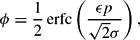
where Θ(s)=0 for s≤0 and Θ(s)=1 for s>0. The variable s is the scale of production of a (representative) firm; hence (16) yields the distribution of si in the economy and ϕ is the fraction of technologies that are active (i.e., such that si>0).
Likewise, the last term on the r.h.s. of equation (14) is related to utility maximization with respect to a “representative” commodity. The variable x is indeed one of the variables xc that appear in the original problem. The solution of this problem is given by

which is always positive, provided
for
. The probability density of xc in the economy can be derived from that of t and x0 in the same way as above for the scale si of production. The conditional probability of xc given x0c is computed in Appendix C. The result is

Hence the variable x−χu′(x) has a Gaussian distribution with mean x0−κ and variance nΔΩ.
The two “representative” problems are coupled in a nontrivial way through the other terms in (14).
The structure of the solution becomes more clear if we analyze the set of saddle point equations
, with
. After some algebra (see Appendix B), these can be cast in the following form:


The first of these equations relates the parameter p to the average (relative) price because of (12), whereas the third one implies that σ is a measure of price fluctuations.4
It is possible to derive an explicit analytic form of (23), (24), and (25) in terms of error functions. The present formulas are, however, more suited for the discussion that follows.
Using these relations (see Appendix D for details), one finds that at the saddle point

This is indeed what we expect when looking at the original problem (11). Furthermore, taking the expected value of (18) and combining it with (20) and (25) yields
. Thus

which is exactly equation (6). Finally, it is possible to show (see Appendix D) that equations (20–25) also “contain” Walras's law in the form

The dependence of the solution on Δ can be clarified by a rescaling argument: changing variables to p′=p,
,
, Ω′=ΔΩ, χ′=χ and κ′=κ one finds that the solution only depends on the parameter ε′=ε/Δ. Hence the behavior of the solution with respect to Δ is easily related to the dependence on ε with Δ=1. Notice that a dependence on Δ remains after the change of variables in the distribution of si, equation (16). This means that production scales satisfy the scaling relation

The behavior of the solution when the spread of the initial endowments
is very small can be computed with asymptotic expansion methods. The key observation in the expansion (see Appendix E) is that x* also has very small fluctuations. This, in turn, implies that prices also have very small fluctuations; indeed
. The scales of production also vanish when
, but with singular exponential behavior,

for some constant A. Hence we find that no economic activity takes place (
,
) in the limit of uniform endowments (see Appendix E for technical details). This is what one should expect from the beginning: when the consumer is endowed with the same amount of equally valued commodities, there is no transformation (with ε≥0) that can increase welfare.
A further interesting limit, for which we can derive generic results, is that of vanishing ε. Setting ε=0, one finds in a straightforward way that
,
, and k=pχ. Equation (7) yields ϕ=1/2, which means that half of the firms are active, in agreement with the geometric argument of the previous section for n<2. When
the equations develop a singularity:
,
vanish, whereas the average scale of production diverges
. A detailed account is given in Appendix F. The case n>2 is more subtle, as it requires a careful asymptotic study of the limit
, where again realizing that x* has small fluctuations of order ε is crucial. The bottom line is that (see Appendix F for details) price fluctuations vanish linearly with ε; that is, σ∝ε but also
, so the factors
and
in equation (15) are finite. Hence scales of production remain finite as
and they diverge when
as
. The fraction of active firms turns out to be ϕ=1/n, which means that there are exactly C firms operating.
Equations (26), (27), and (28) show that the saddle point equations, which represent the simplest mathematical description of the random economy in its full complexity, manage to capture in a compact, though somewhat intricate, way the basic properties of the economy. This is a useful consistency check. The best way to unravel the resulting behavior beyond these generic laws is, however, to specialize to particular cases.
THE SOLUTION: TYPICAL CASES
In this section we display the behavior of the solution outlined in the previous section for some particular choices of the functions u(x) and ρ(x0). In spite of their apparent complexity, equations (20–25) can be solved numerically to any desired degree of accuracy. Using the scaling argument above, we can safely restrict ourselves to studying the dependence on ε, setting Δ=1, without any loss of generality.
We shall henceforth set

We start our discussion from the case

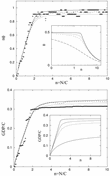
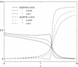
Figure 1 compares the numerical solution with computer experiments. We generate many realizations of the random economy and compute the equilibria for each of them numerically. The analytical results we obtain in the limit C→∞ turn out to give a quite accurate description of the behavior of relatively small systems5
We resorted to a simple iterative scheme to converge to the equilibria. This fails to converge properly for C or N too large or for ε[Lt ]1.

Comparison between the analytic solution for N→∞ (full line) and equilibria of random economies computed numerically for C=16 and 32. The parameters are ε=0.05 and Δ=1, whereas initial endowments are drawn from an exponential distribution. Dots refer to a single realization with C=32, whereas the dotted (dashed) line is the average over 100 realizations for C=16 (32). Top: nϕ, which is the number of active firms (si>0) divided by C, versus n. Bottom: GDP versus n. Insets in these figures show the behavior of ϕ and of GDP for ε=0.01, 0.05, 0.1, and 0.5 from top to bottom.
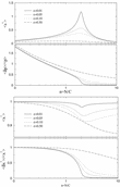
The transition between the two regimes becomes sharper when ε decreases and it gives rise to a singularity in the limit ε → 0, as we have seen in the previous section. This is clearly visible in Figure 2, where we plot the behavior of various quantities as a function of n for different values of ε.

Behavior of equilibrium quantities as a function of n for ε=0.5, 0.1, 0.05, and 0.01. In all cases Δ=1 and ρ(x)=e−x. Top: above, $\avg{s^*}$; below, relative price fluctuations. Here we identify prices with marginal utility p=u′(x*) and $\delta p =u'(x^*)-\avg{u'(x^*)}$. Bottom: above, average consumption $\avg{x^*}$; below, relative fluctuations of consumption $\delta x=x^*-\avg{x^*}$.

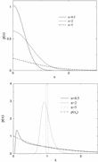
Probability density functions of operation scales s (top) and of consumptions x (bottom) at equilibrium for ε=0.01 and n=0.5, 2, and 5.
For n<nc the average scale of production
increases with n. This means that, in this region, existing firms benefit from the entry of a new technology (i.e., if N→ N+1, see later). This positive complementarity arises because the new firm increases the availability of inputs to other firms.
For n>nc, instead
decreases with n, the introduction of a new technology typically causes a reduction in the scale of activity of the already existing firms. When
the curves develop a singularity
at nc=2, as discussed in the previous section.
As n increases relative price fluctuations decrease. But the decrease becomes very sharp close to nc for ε[Lt ]1. In this case, at nc price fluctuations suddenly drop to a level close to zero. This is related to the behavior of the variable x* shown in the right panel of Figure 2. In the region below nc the average consumption level decreases. In this region firms take advantage of the spread

between scarce and abundant goods to make a living. But as n approaches nc, the spread in x quickly drops to a very low value, making life more difficult. As n increases beyond nc=2, the economy becomes very selective toward increasingly efficient technologies that can perform the desired transformation between commodities with a smaller decrease in the average level
of consumption. This is clearly shown in Figure 2, where we plot the probability densities of x for n=0.5, 2, and 5. The right plot shows that whereas for n=0.5 the distribution P(x|·), equation (19), retains the character of the distribution of initial endowments ρ(x0), it becomes more and more peaked around
as n increases. At the same time the distribution of s, equation (16), becomes broader and broader.
The distribution of si, equation (16), which may be considered as a proxy for firm sizes, gets broader and broader as n increases. Interestingly mature economies, such as Japan [Okuyama et al. (1999)] or the United States [Axtell (2001)], are characterized by a very broad distribution of firm sizes, which we can put in relation to Q(s). The shape of the distribution found empirically is close to a power law, which is different from (16). However, it is not difficult to derive a power law distribution of s by relaxing the unrealistic assumption that all firms have the same value of Δ and ε [De Martino et al. (2004)].
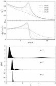
The generic picture of the overall economy depicted thus far remains unchanged for different distributions ρ(x0) of initial endowments or for different utility functions u(x). For example, Figure 4 shows the results obtained with


Top: Scale of production (above) and consumption fluctuations (below) as a function of n for a bimodal distribution of initial endowments (equation 34) with f=0.2 and x0=5 (ε=0.01). Bottom: distribution of x for n=1, 2, and 5.
This captures the situation where only a fraction f of the commodities is present in initial endowments (primary goods), whereas the remaining commodities have to be provided by the productive sector. The behavior of ϕ,
, and relative prices is very similar to that found for the previous model. Figure 4 shows that the average scale of production and the relative fluctuations of xc show qualitatively different behavior. Again, the two regimes with clearly distinct properties can be identified for n<nc and n>nc.
DISCUSSION
The behavior of the solution with n allows us to identify two classes of economies: mature economies (n>2) with a full-blown repertoire of technologies that closely saturate consumers demand and immature economies (n<2) characterized by few technologies scattered in a large space of productive opportunities.
Strictly speaking, our considerations must be limited to comparative statics in view of the static nature of the equilibrium we study. However, it is suggestive to consider dynamic transitions between equilibria. In particular, a transition N→ N+1, corresponding to the draw of a new technology, can be considered as the result of the discovery of a new method of combining inputs to produce desirable outputs, a new design, as Romer (1990) calls it. Note, however, that in Romer's model innovation entails the discovery of a new intermediate commodity and there is no real “combination” of inputs and no heterogeneity across technologies. By contrast, innovation in our model describes the expansion of the frontier of feasible industrial transformation processes by discovery of a new activities which is structurally different from existing ones.6
This is only one of the possible modes of technological innovations. Innovations may also increase the efficiency of an existing technology, e.g., decreasing the input requirements, which may be captured by changes in εi and Δi. Our focus here is on structural technological change.
It has been argued that technological innovation is path-dependent [Dosi (1998)]. This means that the draw of the (N+1)th technology depends on the N technologies that are already present. Such issues can clearly not be addressed within our quasi-static approach.
In such a dynamic view,8
For example, consider the following cartoon of an evolving economy: In each period t nature endows the representative consumer with a bundle x0(t) of commodities, drawn at random from the distribution ρ0. Given the existing technologies,
, this is transformed into the optimal bundle x(t) by the productive sector; then x(t) is consumed at the end of period t. Finally an innovation event, that is, a transition
or
, may take place. It is implicit in this description that technological change occurs on a much longer time scale than that needed for the economy to reach equilibrium. This view may also describe the way in which existing technologies diffuse in a developing country. Technologies are not discovered anew, but just become operative or feasible as, e.g., human capital or infrastructure accumulates, or institutional constraints are removed.

Variation of GDP for $N\to N+1$ (full lines) and for $C\to C+1$ (dashed lines). Here u(x)=log x and $\rho(x_0)=e^{-x_0}$.
The same conclusion can be reached assuming that investment in research arise from the productive sector itself. Indeed, the average scale
of activity of firms increases with n for n<2, which means that a transition N→ N+1 causes an increase in the average scale of activities already active. This means that, at the equilibrium prices of the economy with N<2C technologies, the profits of already existing firms increase on average when the new technology is introduced. Likewise, the decrease of
with n for n>2 suggests that transitions C → C+1 increase firms profits, on average, for n>2. This again yields a drift toward n≈2 due to endogenous technological change.
These arguments suggest that economies may spontaneously evolve toward a critical state, that is, that they may be a further realization of self-organized criticality Bak and Chen (1991).
CONCLUSIONS
Summarizing, we have addressed the problem of calculating the general equilibria of large linear production economies with random technologies and a single consumer with tools of statistical physics. In a nutshell, our results can be stated as follows. When the ratio n of the number of available technologies to the number of commodities is below a threshold nc=2, the average operation scale grows as n increases and roughly one-half of the firms are active. For n<2, new technologies are easily accepted and the economy on the whole expands with n. When n>nc, instead, the production sector is saturated; that is, the number of active technologies converges to the number of commodities, and new technologies are accepted only at the expense of reducing the operation scales of the other technologies. The transition becomes more and more sharp as the parameter ε, measuring the inefficiency of each technology, approaches zero. From the consumer's viewpoint, welfare increases with n in both regimes. The main component of welfare increase with n is different in the two regimes: for n<nc, welfare level grows with n because the spread in consumption levels
decreases with the introduction of technologies that transform abundant commodities into scarce ones. For n>nc, instead, growth arises from the introduction of more efficient technologies, granting an increase in the level of consumption
. Accordingly, the relative spread of prices
decreases with n.
Considering the incentives for technological innovations, we uncover a mechanism by which the economy self-organizes to the critical state ≈2. Our model clearly is unrealistic in many respects. Still, it may capture some novel aspects of structural technological change. The extension of these approaches to a fully dynamic setting, including capital accumulation, may shed new light on theories of endogenous economic growth.
Above all, we propose the use of statistical mechanics of disordered systems to study the typical properties of the general equilibria of large random economies. We have shown how these methods are able to deal effectively with heterogeneity, providing a complete statistical description of the equilibria, which is consistent with generic results. The relevant quantities—called order parameters—are naturally identified by the method. Given the nonstandard type of calculations involved, we also present computer experiments that convincingly support our results.
The approach generalizes in a straightforward way to more complex situations and we hope that this work will stimulate cross-fertilization between the fields of economic theory and statistical mechanics.
APPENDIX A: THE METHOD
The standard technique for maximizing a function of N variables with N→∞ in statistical mechanics relies on the well-known steepest descent, or saddle point, method. Let HN(·) be an extensive function of
(i.e., such that there are two constants k+ and k− satisfying k−N<HN(s)<k+N for all N and s), and imagine that we want to compute the maximum value of HN(s)/N in the limit N→∞. Then

where

is called the partition function associated to HN. Here ∫ds stands for an N-dimensional integral on the whole domain of definition of s. The idea of (A.2) is that the integral for β[Gt ]1 is dominated by regions where HN is maximal. This recipe turns the problem of maximizing h into that of calculating ZN and evaluating the asymptotic behavior of its logarithm.
This task becomes much more difficult when HN depends on a set of random variables q with probability density p(q). We denote this dependence by HN(·|q). The generic situation is that q enters the definition of the interactions among the N components of s and HN is a sum over all interaction terms. In such situations, we expect that a sufficiently regular HN will obey the law of large numbers, so that, e.g.,

In other words, max HN/N is expected to be a self-averaging quantity, namely to have vanishing sample-to-sample fluctuations in the limit N→∞. If one wanted to generalize (A.1) to the evaluation of (A.3), one would have to compute the q-average of the logarithm of the partition function ZN(β | q). Unfortunately, the logarithm prevents every useful factorization of such an average and makes this method impracticable.
The replica method is the standard statistical mechanical technique for circumventing this difficulty. Using the formula

we can reduce our problem to that of computing
. This is feasible for integer values of r because it amounts to computing

which is the partition function of r “replicas” of the original system with the same disorder realization q (hence the name of the method). The last step consists in performing an analytic continuation for real values of r and taking the limit r→ 0:

The existence and uniqueness of the limit r→ 0, which looks somewhat bizarre, have been much debated in the physics literature [see Mezard et al. (1987) for a discussion]. Even if this method remains a formally nonrigorous procedure, several rigorous mathematical results confirm its validity in problems that are more complex that the one we deal with here [Talagrand (1998, 2003)]. We hope this (together with the agreement with computer experiments) gives the reader a sufficient level of confidence to accept the r→ 0 passage.
The technical part of the calculation lies in the introduction of a finite number of auxiliary integration variables
allowing the averaged replicated partition function to be recast in the form

where h(·) is some function and
in the limits
, r→ 0. The
variables are called order parameters. Their nature and number are dictated by the mathematical structure of the problem (see Appendix B for the details in our case). Finally, assuming that the limits r→ 0 and N→∞ commute, the latter can be taken first in (A.6), thus making it possible to evaluate (A.7) by the saddle-point method as

where
is the saddle point value of
that dominates the integral in (A.7). Hence, putting things together,

The core of the procedure lies in (A.7), where, by a lengthy calculation, one identifies the relevant order parameters
and the function h. This crucial but technical step is presented below (Appendix B) for our problem.
APPENDIX B: THE EXPLICIT CALCULATION OF THE REPRESENTATIVE AGENT PROBLEM
The partition function in our case reads

with U(x) the utility function of the representative consumer. As stated above, in order to analyze the statistical properties of the equilibria, we have to evaluate
and resort to (A.6), with HN given in our case by U and with all the necessary constraints. Before proceeding, we shall introduce some useful definitions and identities. The first one is the δ-function δ(x), which is defined through the relation

for any function f(·) and y∈R. We will also use the exponential representation of the δ-function,

Another mathematical tool we will use is the Gaussian or Hubbard–Stratonovich transformation, viz.,

which makes it possible to linearize arguments of exponentials at the cost of introducing averages over Gaussian random variables. Now, to perform our calculation, it is convenient to replace the consumption variables x by writing explicitly the market-clearing condition (4) in the partition function (B.1). To do so we use the defining property (B.2) of δ-distributions and write

As already explained in Appendix A, we will have to take the following steps: (a) average the partition function of r replicas over technologies, as in (A.7); (b) identify the correct order parameters of the problem to write the latter average, as in (A.7); (c) take the limits N→∞ and r→ 0 and get something of the form of (A.9); and finally (d) find the values of the order parameters at the competitive equilibrium (i.e., when
).
The partition function of r replicas reads

Notice that the dependence on the technologies appears in the market-clearing condition only, so that the average
involves only the last part of [ZN(β | q)]r. This average must take into account the constraint (1), that is,

where
stands for the average over unconstrained i.i.d. Gaussian vectors
with zero mean and variance
. Using equation (B.3) for the constraints, the denominator becomes

whereas for the numerator we get

Note that the expected values involved in these calculations are all of the form
. This is the characteristic function of
, and for the assumed Gaussian distribution, it takes the form
. This result can, however, be extended to any distribution of
with
with a leading behavior
. Indeed, all higher order terms in the power expansion of
give vanishingly small contributions with respect to the first, in the limit C→∞.
Gathering all the terms, we have

In order to write the above in a form as simple as (A.7), the set of order parameters to be introduced must allow a decoupling of the integrals over the variables
, si,a, and
in such a way that the integrals on the different variables can be factorized. Here it is enough to introduce the order parameters

through identities such as

Then the last term in the exponent of the numerator of equation (B.10) becomes

This allows us to separate the problem into three parts. Indeed we can re-cast the replicated partition function in the form of a set of integrals over the order parameters,

where h=g1+g2+g3 is the sum of three terms that can be computed independently:


with n=N/C. The order parameters
have appeared after using an identity similar to (B.12) for ka. Now (B.14) is precisely of the form (A.7).
In the limit N→∞ the integrals appearing in (B.14) are dominated by the contributions coming from the saddle point of h and the solution of our specific problem can be written as

where the * means that parameters take their saddle point values that is, those that solve the system of equations

for all a, b=1, …, r. Ideally one should first solve these equations for generic r and then take the limit as r→ 0.
A word about the meaning of the order parameters introduced thus far is in order before taking the limit r→ 0. Indeed, ωab is an r×r matrix for integer r, but it is not clear how can we handle it in the limit r→ 0. When we replicated the partition function passing from (B.1) to (B.6) we essentially passed from a problem in which U(xa) is to be maximized to an equivalent problem in which [sum ]aU(xa) is to be maximized. The latter sum is evidently left unchanged by a permutation of the replica indexes 1, …, r. Hence it must be expected that, as long as there is a unique maximum (as in this case), replica permutation symmetry is preserved also by the solution of equations (B.19). Then we expect a solution of the form

This is the so-called replica-symmetric Ansatz, which simply expresses the conservation of the permutation symmetry. When multiple maxima with different statistical properties exist, this Ansatz fails because replicas can converge to maxima with different properties, and hence replicas are no longer equivalent. This situation is ruled out in our case by the nature of the function we want to maximize.
With equations (B.20), it is easy to find an analytic expression for the functions g1, g2, and g3 in terms of r and to perform the limit r→ 0. Substituting (B.20) into the definitions of g1, g2, and g3, after some straightforward algebraic manipulations one finds


where


We must finally evaluate the limit
. In this limit, a somewhat special role is played by the quantity χ=β(Ω−ω). Notice that

is the distance between two replicas. The two vectors sa and sb both converge to the unique solution of the maximization problem as
. Hence, we also expect the distance Ω−ω to vanish in this limit. But looking, e.g., at W/β one realizes that to avoid annoying divergences or trivial limits this quantity must vanish in such a way that the product β(Ω−ω) stays finite. In other terms, one wants Ω−ω∼1/β for large β. If this is the case, the maximization problem has a well-defined solution. Hence we assume that
is finite. Similar arguments lead to the introduction of the following redefined order parameters, which remain finite as
:


Inserting these into the previous expressions, we find that the r.h.s. of (B.18) (which we for simplicity denote again by h) can be written as

where now the functions V and W read


We neglect the last term in W because it is vanishingly small in the limit
when χ is finite.
When
, again by steepest descent reasoning, only the maxima of V and W contribute to the integrals over s and x. Therefore we can write the final expression for h as

The difference between this expression and the one appearing in (14) is again a trivial redefinition of the order parameters. If we let now x*(t, x0) and s*(t) be the values maximizing the functions W and V, respectively, and therefore given by (15) and (18), we can then expand (B.32) to obtain

The last step is to derive the saddle-point equations from which the values that the order parameters take on at equilibrium can be calculated. Computing the derivatives of h with respect to the order parameters, we get


Using the relation (18) and setting
,
, we finally arrive at equations (20–25).
APPENDIX C: THE PDF'S OF s AND x
We illustrate here the procedure for calculating the conditional probability density of x (the equilibrium consumption) given x0 (the initial endowment). The derivation of the distribution of s follows exactly the same lines. One can start from the identity

Then one can make use of the property δ(x−x*)=|f′(x*)|δ[f(x)], where f(x) is a function with a unique root in x*. From (18), we take

so that

From this, taking the integral over t, one immediately finds (19).
APPENDIX D: CALCULATION OF h AT THE SADDLE POINT AND DERIVATION OF WALRAS'S LAW
Replacing s with s*(t) (15) and x with x*(t, x0) (18), we can rewrite h as

Now it is a simple algebraic problem. For the first term on the r.h.s. we use (25); for the second and the fifth we use (25); the third and fourth cancel because of (23); finally, for the last term, we use (18) and then (22) to find

(26) follows immediately.
In order to derive Walras' law, we note that when computing
, one can make the substitution
(which is only valid when s*>0). Then (25) becomes

where we have used 25 in the last equality. Likewise, we can substitute for t in the average of (21) by solving (18) for t. This yields

which can be substituted back into (D.3). This yields the desired result (28).
APPENDIX E: ALMOST UNIFORM INITIAL ENDOWMENTS
In this section we study the limiting behavior of the economy when the spread of initial endowments is vanishingly small. In particular, we show that when the initial distribution of endowments becomes uniform the volume of productive activity vanishes. We take Δ=1 for simplicity. We take
, with
a fixed value and δx0 a small random variable, and discuss the solution to the leading order in
. Then, taking
we can write, to leading order in δx0 and δx*,

From here we can identity the zeroth and first-order terms in δx*, viz.,

Then from equation (21) we get

and from equation (22)

Coming to the equations for Ω and χ we observe that s*(t)=s0(t−τ)Θ(t−τ), where


Then we can write
with
, which can be solved for Ω

Careful asymptotic analysis implies that in the limit of vanishing fluctuations
of the initial endowment τ diverges as

Using asymptotic expansion for I(τ), one finds that the leading-order behavior of Ω is

Analogously, for χ, we have

With these we finally get
and
. Therefore, when the fluctuations of the initial endowment vanish, there is no market activity.
APPENDIX F: LIMIT ε → 0
Setting ε=0, the averages over s*(t) become trivial and equations (23–25) are easily evaluated. Progress with the other equations is possible, for generic u(x) and ρ(x0), close to n=2. We expect that the consumption vector x is nearly constant. Then, as in the previous case, we assume that
with δx* small. Thus
as before. Using the expressions for Ω, χ, and κ and expanding equation (18) to linear order as above, we find the expression

where
. This allows us to compute
and hence to evaluate equation (21):

Likewise we can evaluate equation (22) and find
. Using these in equations (15,23) we find the divergence of Ω≅1/(2−n).
This solution breaks down for n>2. We need to take the limit
carefully into account. Again we anticipate that the spread δx* will be small. More precisely, we assume that σ and
vanish linearly with ε, set
and σ=dε, and look for a solution with finite s0 and d. The existence of such a solution justifies our assumption. Then
, where
has already been introduced above. The equation for χ yields χ=nΔs0J(p/d)/(dε), where
. Expanding equation (18), as in the previous section, and using the expressions for Ω and χ just derived, we find

which justifies our a priori assumption of small fluctuations. Inserting this and the expressions for Ω in equation (21) for
, after some manipulations, one finds

which gives d as a function of n and
. Notice that ϕ=J(p/d)=1/n. Furthermore, J(τ)≤1/2 for τ≥0, which means that this solution describes the region n≥2. This equation also simplifies the expression of χ≅Δs0/(dε). The equation for σ finally gives

Note that equation (F.4) implies that
as
. The leading behavior is
. In the same limit
, which means that
also diverges as
, matching the divergence for
.
We are indebted to A. Bigano, D. Fiaschi, K.-G. Maler, F. Vega-Redondo, and M.A. Virasoro for useful discussions and to The Abdus Salam ICTP for hospitality and support within a thematic institute of the EU EXYSTENCE network of excellence. This work was supported in part by the European Community's Human Potential Programme under Contract HPRN-CT-2002-00319, STIPCO. IPC thanks the Fund for Scientific Research-Flanders, Belgium.