1 Introduction
One of the major advances in convection-driven dynamos over the last decade has been the ability of the numerical simulations to reproduce some of the observed features of the Earth’s magnetic field, such as a strongly dipolar magnetic field aligned with the rotation axis, occasional reversals in polarity and a slow westward drift of the surface magnetic field (Christensen Reference Christensen2010). This is all the more astonishing as the parameter regime in the numerical experiments is very far from that in the core of the Earth. For example, the simulations are much too viscous, typically by a factor of
 $10^{9}$
as measured by the Ekman number, and substantially underpowered, as measured by the ratio of the Rayleigh number to the critical Rayleigh number at which convection first sets in (Christensen & Wicht Reference Christensen, Wicht and Olson2007; Christensen Reference Christensen2011). There is, therefore, a growing need to understand exactly what dynamical mechanisms these numerical experiments embrace which allows them to capture planet-like behaviour, despite the fact that many aspects of the simulations are distinctly not planet-like.
It was recognised early in dynamo theory that an important ingredient of a dipolar planetary dynamo is the breaking of reflectional symmetry (Moffatt Reference Moffatt1978), and in the numerical simulations of such dynamos this usually takes the form of an abundance of kinetic helicity,
 $h=\boldsymbol{u}\boldsymbol{\cdot }\unicode[STIX]{x1D735}\times \boldsymbol{u}=\boldsymbol{u}\boldsymbol{\cdot }\unicode[STIX]{x1D74E}$
, in the convective flow (Roberts & King Reference Roberts and King2013). Moreover, an efficient dynamo requires that the mean helicity is spatially segregated, being of one sign in the northern hemisphere and another sign in the south. Precisely such an asymmetric distribution in the azimuthally averaged helicity was observed quite early in the numerical simulations (Olson, Christensen & Glatzmaier Reference Olson, Christensen and Glatzmaier1999), and indeed it occurs even in the absence of a magnetic field (Glatzmaier & Olson Reference Glatzmaier and Olson1993; Kitauchi, Araki & Kida Reference Kitauchi, Araki and Kida1997). In particular, outside the tangent cylinder (an imaginary cylinder that circumscribes the solid inner core and is parallel with the rotation vector,
 $\unicode[STIX]{x1D734}$
), the helicity is observed to be negative in the north and positive in the south. This is important because nearly all of the current numerical dynamos operate outside the tangent cylinder (Christensen Reference Christensen2011). So, two important questions are: what basic mechanism is responsible for the generation and subsequent spatial segregation of helicity in the numerical simulations, and why is it predominantly negative in the north and positive in the south (outside the tangent cylinder)? To date, these questions remain unanswered.
The production and segregation of helicity was attributed to Ekman pumping in some of the early simulations (Kono, Sakuraba & Ishida Reference Kono, Sakuraba and Ishida2000; Roberts & King Reference Roberts and King2013), but these simulations were particularly viscous and weakly forced, and this has now been largely abandoned as a realistic mechanism. For example, it is not the primary source of helicity in slightly less viscous simulations (Olson et al.
Reference Olson, Christensen and Glatzmaier1999), it plays almost no role whatsoever in the most recent low Ekman number numerical simulations (Schaeffer et al.
Reference Schaeffer, Jault, Nataf and Fournier2017), and numerical simulations involving slip boundary conditions, in which there can be no Ekman pumping, also produce dipolar dynamos (Kageyama, Watanabe & Sato Reference Kageyama, Watanabe and Sato1993; Yadav, Gastine & Christensen Reference Yadav, Gastine and Christensen2013). Moreover, Ekman pumping is unlikely to play any role at all in planetary cores, where the Ekman number is tiny,
 ${\sim}10^{-15}$
in the case of the Earth.
Given that the Earth rotates rapidly with a low convective Rossby number,
 $Ro=u/\unicode[STIX]{x1D6FA}l\ll 1$
, it has long been recognised that an alternative source of helicity may be the propagation of helical waves supported by the Coriolis force (Moffatt Reference Moffatt1970; Olson Reference Olson1981). The point is that, while a low value of
 $Ro$
demands that
 $\boldsymbol{u}\boldsymbol{\cdot }\unicode[STIX]{x1D735}\boldsymbol{u}$
is much weaker than the Coriolis force, we have no right to similarly neglect
 $\unicode[STIX]{x2202}\boldsymbol{u}/\unicode[STIX]{x2202}t$
, as there is no a priori reason why the time derivative should scale on the convective time, and as soon as we allow for a non-negligible
 $\unicode[STIX]{x2202}\boldsymbol{u}/\unicode[STIX]{x2202}t$
, waves are inevitable. This idea was taken up again in Davidson (Reference Davidson2014) and Davidson & Ranjan (Reference Davidson and Ranjan2015), who focused particularly on the simplest type of helical wave – inertial waves. The hypothesis put forward in Davidson (Reference Davidson2014) and Davidson & Ranjan (Reference Davidson and Ranjan2015) is that most planets are rapid rotators and so are natural wave-bearing systems which are almost certainly awash with helical waves, such as inertial waves and magnetostrophic waves. In particular, it is argued that fast inertial waves are required to maintain the approximate geostrophy observed in the simulations, a quasi-geostrophy that is maintained despite the chaotic evolution of the thermal forcing and the turbulent nature of the resulting velocity field. Moreover, outside the tangent cylinder the temperature perturbations and buoyancy flux, which act as triggers for helical waves, are observed to be concentrated in and around the equatorial plane. This was noticed as early as Gilman (Reference Gilman1977) and then later by Glatzmaier & Olson (Reference Glatzmaier and Olson1993). This is illustrated in figure 1(a), which is taken from Sakuraba & Roberts (Reference Sakuraba and Roberts2009) and shows the computed radial velocity in one of their simulations. It is also evident in figure 1(b), which is from Ranjan et al. (Reference Ranjan, Davidson, Christensen and Wicht2018) and shows the computed root-mean-square (r.m.s.) azimuthal temperature gradient, averaged in the azimuth. In both of these cases the primary source of excitation for waves lies in the equatorial regions. This is significant because upward propagating helical waves, either inertial or magnetostrophic waves, are known to carry negative helicity, while downward propagating helical waves carry positive helicity (Moffatt Reference Moffatt1978). So waves triggered in and around the equatorial plane will tend to support negative helicity in the north and positive helicity in the south, exactly as seen in the numerical simulations (figure 1
c), and exactly as required for dynamo action.
(a) The computed radial velocity in one of the simulations of Sakuraba & Roberts (Reference Sakuraba and Roberts2009). (b) The r.m.s. azimuthal temperature gradient, averaged in the azimuth, in the simulation of Ranjan et al. (Reference Ranjan, Davidson, Christensen and Wicht2018). (c) The helicity distribution in a simulation by Schaeffer et al. (Reference Schaeffer, Jault, Nataf and Fournier2017).

There is a second, intriguing feature of the numerical simulations that requires some explanation. As noted in Davidson & Ranjan (Reference Davidson and Ranjan2015), it is possible to write a low
 $Ro$
evolution equation for the helicity of the form
 $$\begin{eqnarray}\frac{\unicode[STIX]{x2202}}{\unicode[STIX]{x2202}t}(\boldsymbol{u}\boldsymbol{\cdot }\unicode[STIX]{x1D74E})=-\unicode[STIX]{x1D735}\boldsymbol{\cdot }\boldsymbol{F}+S_{h}.\end{eqnarray}$$
The origins and interpretation of this equation are spelt out in § 2, where it is shown that
 $\boldsymbol{F}$
is a wave flux involving the Coriolis force, and hence
 $\unicode[STIX]{x1D734}$
, while the source term,
 $S_{h}$
, is a function of
 $\boldsymbol{u}(\boldsymbol{x},t)$
and of those buoyancy fluctuations which act as triggers for helical waves. A comparison of the azimuthally averaged distributions of
 $h$
and
 $S_{h}$
in a numerical dynamo is shown in figure 2(a,b), where (a) is taken from Ranjan et al. (Reference Ranjan, Davidson, Christensen and Wicht2018) and (b) has been calculated from the same data set. It is extraordinary how close the azimuthally averaged spatial distributions of
 $h$
and
 $S_{h}$
are. At first sight this argues for an in situ generation of helicity, such as the quasi-static mechanism suggested by Hide (Reference Hide1976), rather than the dispersal of helicity by waves. Curiously, though, no such correlation is observed between
 $\unicode[STIX]{x2202}h/\unicode[STIX]{x2202}t$
and
 $S_{h}$
in the same numerical simulation (figure 2
c). This suggests that there may be an alternative explanation for the observed correlation between
 $h$
and
 $S_{h}$
, and we shall argue here that this is indeed the case. Specifically, we shall show the source term in (1.1) automatically adjusts to take the same sign as the prevailing helical wave flux. That is to say,
 $S_{h}$
is not independently prescribed, but is itself shaped by the wave dynamics.
A comparison of the azimuthally averaged values of
 $h$
,
 $S_{h}$
and
 $\unicode[STIX]{x2202}h/\unicode[STIX]{x2202}t$
in (1.1). Panel (a) is taken from Ranjan et al. (Reference Ranjan, Davidson, Christensen and Wicht2018) and (b,c) have been calculated from the same data set.

Because of the presence of both an ambient magnetic field and a background rotation, there are several classes of helical waves which might exist in the core of a planet. However, these share many common features and differ mostly in their time scales (Moffatt Reference Moffatt1978). Consequently, we shall follow Davidson & Ranjan (Reference Davidson and Ranjan2015) and focus on the simplest case – that of inertial waves. In the parlance of dynamo theory, we consider the weak-field regime. Our primary task is to test the hypothesis that the antisymmetric distribution in
 $h$
observed in the numerical simulations, as well as the spatial correlation between
 $h$
and
 $S_{h}$
in (1.1), could arise from the spontaneous emission of inertial waves from buoyant anomalies. Because the numerical simulations exhibit highly complex dynamics, with many distinct physical processes occurring simultaneously on multiple time scales, we restrict ourselves to a sequence of idealised model problems, designed to expose the underlying dynamics.
2 The equations governing the dispersal of helicity from a localised source of buoyancy
2.1 Inertial waves at low Rossby number
We consider a rapidly rotating, Boussinesq fluid at low Rossby number,
 $Ro=u/2\unicode[STIX]{x1D6FA}\ell \ll 1$
, in which motion is driven by density anomalies. The governing equations of motion in the rotating frame of reference are
 $$\begin{eqnarray}\displaystyle & \displaystyle \frac{\unicode[STIX]{x2202}\boldsymbol{u}}{\unicode[STIX]{x2202}t}=2\boldsymbol{u}\times \unicode[STIX]{x1D734}-\unicode[STIX]{x1D735}(p/\unicode[STIX]{x1D70C})+\unicode[STIX]{x1D717}\boldsymbol{g}+\unicode[STIX]{x1D708}\unicode[STIX]{x1D6FB}^{2}\boldsymbol{u}, & \displaystyle\end{eqnarray}$$
 $$\begin{eqnarray}\displaystyle & \displaystyle \unicode[STIX]{x1D735}\boldsymbol{\cdot }\boldsymbol{u}=0, & \displaystyle\end{eqnarray}$$
where
 $\unicode[STIX]{x1D734}=\unicode[STIX]{x1D6FA}\hat{\boldsymbol{e}}_{z}$
is the background rotation,
 $p$
is pressure,
 $\unicode[STIX]{x1D708}$
the viscosity,
 $\unicode[STIX]{x1D70C}$
the background density,
 $\boldsymbol{g}$
is gravity,
 $\unicode[STIX]{x1D717}=\unicode[STIX]{x1D70C}^{\prime }/\unicode[STIX]{x1D70C}$
and
 $\unicode[STIX]{x1D70C}^{\prime }$
is the perturbation in density. We have in mind cases where
 $\boldsymbol{g}$
is perpendicular to
 $\unicode[STIX]{x1D734}$
, reminiscent of a buoyant anomaly sitting near the equatorial plane of the Earth’s core, and we take
 $\unicode[STIX]{x1D70C}^{\prime }$
to be negative, in line with the notion of buoyant anomalies floating out towards the mantle in the core.
If we introduce a solenoidal vector potential,
 $\boldsymbol{a}$
, for the velocity,
 $\boldsymbol{u}=\unicode[STIX]{x1D735}\times \boldsymbol{a}$
, then we may rewrite (2.1), and its curl, in the alternative form
 $$\begin{eqnarray}\displaystyle & \displaystyle \frac{\unicode[STIX]{x2202}\boldsymbol{u}}{\unicode[STIX]{x2202}t}=2\unicode[STIX]{x1D734}\boldsymbol{\cdot }\unicode[STIX]{x1D735}\boldsymbol{a}-\unicode[STIX]{x1D735}(p^{\ast }/\unicode[STIX]{x1D70C})+\unicode[STIX]{x1D717}\boldsymbol{g}+\unicode[STIX]{x1D708}\unicode[STIX]{x1D6FB}^{2}\boldsymbol{u}, & \displaystyle\end{eqnarray}$$
 $$\begin{eqnarray}\displaystyle & \displaystyle \frac{\unicode[STIX]{x2202}\unicode[STIX]{x1D74E}}{\unicode[STIX]{x2202}t}=2\unicode[STIX]{x1D734}\boldsymbol{\cdot }\unicode[STIX]{x1D735}\boldsymbol{u}+\unicode[STIX]{x1D735}\unicode[STIX]{x1D717}\times \boldsymbol{g}+\unicode[STIX]{x1D708}\unicode[STIX]{x1D6FB}^{2}\unicode[STIX]{x1D74E}, & \displaystyle\end{eqnarray}$$
where
 $$\begin{eqnarray}\unicode[STIX]{x1D6FB}^{2}(p^{\ast }/\unicode[STIX]{x1D70C})=\unicode[STIX]{x1D735}\boldsymbol{\cdot }(\unicode[STIX]{x1D717}\boldsymbol{g}).\end{eqnarray}$$
The buoyancy field,
 $\unicode[STIX]{x1D717}$
, is assumed to be advected by a simple advection diffusion equation, with a diffusivity
 $\unicode[STIX]{x1D705}$
equal to that of the kinematic viscosity. From (2.1) we see that
 $u\sim \unicode[STIX]{x1D717}g/\unicode[STIX]{x1D6FA}$
, and so a characteristic Rossby number is
 $Ro=\unicode[STIX]{x1D717}_{0}g/2\unicode[STIX]{x1D6FA}^{2}\unicode[STIX]{x1D6FF}$
, where
 $\unicode[STIX]{x1D717}_{0}$
is a characteristic density fluctuation and
 $\unicode[STIX]{x1D6FF}$
is a typical length scale for the buoyancy field.
We are interested in how energy and helicity disperse from localised buoyancy sources at low Ekman numbers. In the absence of viscosity, and away from buoyancy sources, (2.3) supports inertial waves governed by the wave-like equation
 $$\begin{eqnarray}\frac{\unicode[STIX]{x2202}^{2}}{\unicode[STIX]{x2202}t^{2}}(\unicode[STIX]{x1D6FB}^{2}\boldsymbol{u})+4(\unicode[STIX]{x1D734}\boldsymbol{\cdot }\unicode[STIX]{x1D735})^{2}\boldsymbol{u}=\mathbf{0},\end{eqnarray}$$
which allows for plane waves of the form
 $\boldsymbol{u}=\hat{\boldsymbol{u}}\exp [j(\boldsymbol{k}\boldsymbol{\cdot }\boldsymbol{x}-\unicode[STIX]{x1D71B}t)]$
. These have the dispersion relationship
 $$\begin{eqnarray}\unicode[STIX]{x1D71B}=\pm 2(\boldsymbol{k}\boldsymbol{\cdot }\unicode[STIX]{x1D734})/k,\quad k=|\boldsymbol{k}|,\end{eqnarray}$$
with
 $0\leqslant \unicode[STIX]{x1D71B}\leqslant 2\unicode[STIX]{x1D6FA}$
and the lowest frequency corresponding to horizontal wave vectors,
 $\boldsymbol{k}\boldsymbol{\cdot }\unicode[STIX]{x1D734}=0$
. The group velocity of inertial waves is then
 $$\begin{eqnarray}\boldsymbol{c}_{g}=\frac{\unicode[STIX]{x2202}\unicode[STIX]{x1D71B}}{\unicode[STIX]{x2202}k_{i}}=\pm 2\frac{\boldsymbol{k}\times (\unicode[STIX]{x1D734}\times \boldsymbol{k})}{|\boldsymbol{k}|^{3}}=\pm 2\frac{k^{2}\unicode[STIX]{x1D734}-(\boldsymbol{k}\boldsymbol{\cdot }\unicode[STIX]{x1D734})\boldsymbol{k}}{|\boldsymbol{k}|^{3}}.\end{eqnarray}$$
Note, in particular, that
 $$\begin{eqnarray}\boldsymbol{c}_{\boldsymbol{g}}\boldsymbol{\cdot }\unicode[STIX]{x1D734}=\pm 2k^{-3}[k^{2}\unicode[STIX]{x1D734}^{2}-(\boldsymbol{k}\boldsymbol{\cdot }\unicode[STIX]{x1D734})^{2}],\end{eqnarray}$$
which tells us that the positive sign in (2.7) corresponds to wave energy travelling upward, while the negative sign corresponds to energy propagating downward.
Note also that low-frequency waves have a group velocity of
 $\boldsymbol{c}_{\boldsymbol{g}}=\pm 2\unicode[STIX]{x1D734}/k$
, and so
 $u/c_{g}\sim Ro$
. It follows that, at low
 $Ro$
, the buoyancy field, and hence
 $p^{\ast }$
, may be regarded as quasi-static on the time scale of the wave dispersion. Inverting (2.5) tells us that this quasi-static pressure field falls off with distance as
 $\unicode[STIX]{x1D735}p^{\ast }\sim |\boldsymbol{x}|^{-3}$
from a localised source of buoyancy. This is faster than the radiation field, which falls as
 $|\boldsymbol{u}|\sim |\boldsymbol{x}|^{-1}$
for on-axis radiation (radiation parallel to
 $\pm \unicode[STIX]{x1D734}$
) and
 $|\boldsymbol{u}|\sim |\boldsymbol{x}|^{-3/2}$
for off-axis radiation (see Davidson, Staplehurst & Dalziel Reference Davidson, Staplehurst and Dalziel2006; Davidson Reference Davidson2013).
Inertial waves have a non-zero helicity,
 $h=\boldsymbol{u}\boldsymbol{\cdot }\unicode[STIX]{x1D74E}$
. This follows from (2.4) combined with the dispersion relationship (2.7), which yields
 $\hat{\unicode[STIX]{x1D74E}}=\mp |\boldsymbol{k}|\hat{\boldsymbol{u}}$
, where
 $\hat{\unicode[STIX]{x1D74E}}$
is the amplitude of the vorticity in the wave. Evidently the vorticity and velocity fields are parallel and in phase, and so monochromatic inertial waves have maximum possible helicity, with the positive sign in (2.9) corresponding to negative helicity, and the negative sign to positive helicity (Moffatt Reference Moffatt1978). Although this argument applies only to a single Fourier mode, wave packets containing a range of wavenumbers also have a high relative helicity, and of the sign expected for a monochromatic wave (Davidson & Ranjan Reference Davidson and Ranjan2015; Ranjan Reference Ranjan2017). Thus, when wave packets disperse from a localised disturbance, waves with negative helicity propagate upward,
 $\boldsymbol{c}_{g}\boldsymbol{\cdot }\unicode[STIX]{x1D734}>0$
, while those with positive helicity travel downward,
 $\boldsymbol{c}_{g}\boldsymbol{\cdot }\unicode[STIX]{x1D734}<0$
.
2.2 An inviscid evolution equation for helicity
We are interested in how helicity disperses from localised sources of buoyancy. As noted in Davidson & Ranjan (Reference Davidson and Ranjan2015), we can obtain an evolution equation for
 $h$
by taking the dot product of
 $\unicode[STIX]{x1D74E}$
with (2.3), the product of
 $\boldsymbol{u}$
with (2.4) and then adding the two equations. Ignoring viscosity, this yields
 $$\begin{eqnarray}\frac{\unicode[STIX]{x2202}}{\unicode[STIX]{x2202}t}(\boldsymbol{u}\boldsymbol{\cdot }\unicode[STIX]{x1D74E})=\{\unicode[STIX]{x1D734}\boldsymbol{\cdot }\unicode[STIX]{x1D735}(\boldsymbol{u}^{2})+(2\unicode[STIX]{x1D734}\boldsymbol{\cdot }\unicode[STIX]{x1D735}\boldsymbol{a})\boldsymbol{\cdot }\unicode[STIX]{x1D74E}\}-\unicode[STIX]{x1D735}\boldsymbol{\cdot }(p^{\ast }\unicode[STIX]{x1D74E}/\unicode[STIX]{x1D70C})+\boldsymbol{u}\boldsymbol{\cdot }(\unicode[STIX]{x1D735}\unicode[STIX]{x1D717}\times \boldsymbol{g})+\unicode[STIX]{x1D74E}\boldsymbol{\cdot }(\unicode[STIX]{x1D717}\boldsymbol{g}).\end{eqnarray}$$
The two terms arising from the Coriolis force may be rewritten as a divergence,
 $$\begin{eqnarray}\unicode[STIX]{x1D734}\boldsymbol{\cdot }\unicode[STIX]{x1D735}(\boldsymbol{u}^{2})+(2\unicode[STIX]{x1D734}\boldsymbol{\cdot }\unicode[STIX]{x1D735}\boldsymbol{a})\boldsymbol{\cdot }\unicode[STIX]{x1D74E}=\unicode[STIX]{x1D735}\boldsymbol{\cdot }((2\boldsymbol{u}^{2})\unicode[STIX]{x1D734}+\boldsymbol{u}\times (2\unicode[STIX]{x1D734}\boldsymbol{\cdot }\unicode[STIX]{x1D735}\boldsymbol{a})),\end{eqnarray}$$
while it will be convenient to rewrite the source terms involving buoyancy as
 $$\begin{eqnarray}\boldsymbol{u}\boldsymbol{\cdot }(\unicode[STIX]{x1D735}\unicode[STIX]{x1D717}\times \boldsymbol{g})+\unicode[STIX]{x1D74E}\boldsymbol{\cdot }(\unicode[STIX]{x1D717}\boldsymbol{g})=\unicode[STIX]{x1D735}\boldsymbol{\cdot }(\boldsymbol{u}\times (\unicode[STIX]{x1D717}\boldsymbol{g}))+2\boldsymbol{g}\boldsymbol{\cdot }(\boldsymbol{u}\times \unicode[STIX]{x1D735}\unicode[STIX]{x1D717}).\end{eqnarray}$$
Our evolution equation for helicity can therefore be written symbolically as
 $$\begin{eqnarray}\frac{\unicode[STIX]{x2202}}{\unicode[STIX]{x2202}t}(\boldsymbol{u}\boldsymbol{\cdot }\unicode[STIX]{x1D74E})=-\unicode[STIX]{x1D735}\boldsymbol{\cdot }\boldsymbol{F}+S_{h},\end{eqnarray}$$
where the flux,
 $\boldsymbol{F}$
, and helicity source,
 $S_{h}$
, are
 $$\begin{eqnarray}\boldsymbol{F}=-(2\boldsymbol{u}^{2})\unicode[STIX]{x1D734}-2\boldsymbol{u}\times (\unicode[STIX]{x1D734}\boldsymbol{\cdot }\unicode[STIX]{x1D735}\boldsymbol{a})+p^{\ast }\unicode[STIX]{x1D74E}/\unicode[STIX]{x1D70C},\end{eqnarray}$$
and
 $$\begin{eqnarray}S_{h}=S_{1}+S_{2}=\unicode[STIX]{x1D735}\boldsymbol{\cdot }(\boldsymbol{u}\times (\unicode[STIX]{x1D717}\boldsymbol{g}))+2\boldsymbol{g}\boldsymbol{\cdot }(\boldsymbol{u}\times \unicode[STIX]{x1D735}\unicode[STIX]{x1D717}).\end{eqnarray}$$
Note that
 $S_{1}$
integrates to zero over a spherical domain, although
 $S_{2}$
need not. We shall now examine the flux,
 $\boldsymbol{F}$
, and source,
 $S_{h}$
, individually.
2.3 The flux term in the helicity equation
Well removed from a localised source of buoyancy the quasi-static modified pressure is weak,
 $p^{\ast }\sim |\boldsymbol{x}|^{-2}$
, and so, to leading order in
 $|\boldsymbol{x}|^{-1}$
, equations (2.13) and (2.14) can be approximated by
 $$\begin{eqnarray}\frac{\unicode[STIX]{x2202}}{\unicode[STIX]{x2202}t}(\boldsymbol{u}\boldsymbol{\cdot }\unicode[STIX]{x1D74E})=-\unicode[STIX]{x1D735}\boldsymbol{\cdot }\boldsymbol{F},\quad \boldsymbol{F}\approx -(2\boldsymbol{u}^{2})\unicode[STIX]{x1D734}-\boldsymbol{u}\times \frac{\unicode[STIX]{x2202}\boldsymbol{u}}{\unicode[STIX]{x2202}t}.\end{eqnarray}$$
Moreover, we shall see in § 3 that dispersion from a localised buoyancy source is usually dominated by low-frequency wave packets,
 $\boldsymbol{k}\boldsymbol{\cdot }\unicode[STIX]{x1D734}\approx 0$
, and in such cases
 $\unicode[STIX]{x1D71B}\ll \unicode[STIX]{x1D6FA}$
, so that the helicity flux is simply
 $\boldsymbol{F}\approx -(2\boldsymbol{u}^{2})\unicode[STIX]{x1D734}$
. This is consistent with upward propagating wave packets carrying with them negative helicity and downward propagating wave packets transporting positive helicity. To see why this is so, suppose the buoyancy source is localised near the plane
 $z=0$
, say confined to the region
 $-\unicode[STIX]{x1D6FF}<z<\unicode[STIX]{x1D6FF}$
. If we integrate (2.13) over all space that lies above the horizontal plane
 $z=\ell \gg \unicode[STIX]{x1D6FF}$
, then we obtain
 $$\begin{eqnarray}\frac{\text{d}}{\text{d}t}\int \boldsymbol{u}\boldsymbol{\cdot }\unicode[STIX]{x1D74E}\,\text{d}V=-\oint _{S}\boldsymbol{F}\boldsymbol{\cdot }\text{d}\boldsymbol{S}\approx -2\unicode[STIX]{x1D6FA}\int _{z=\ell }\boldsymbol{u}^{2}\,\text{d}A.\end{eqnarray}$$
Similarly, integrating (2.13) over all space that lies below the horizontal plane
 $z=-\ell$
yields
 $$\begin{eqnarray}\frac{\text{d}}{\text{d}t}\int \boldsymbol{u}\boldsymbol{\cdot }\unicode[STIX]{x1D74E}\,\text{d}V=-\oint _{S}\boldsymbol{F}\boldsymbol{\cdot }\text{d}\boldsymbol{S}\approx 2\unicode[STIX]{x1D6FA}\int _{z=-\ell }\boldsymbol{u}^{2}\,\text{d}A.\end{eqnarray}$$
So we obtain negative helicity above the source and positive helicity below, as expected from an analysis of monochromatic waves.
More generally, if we are remote from all sources of buoyancy, and we consider only the helicity transported by the fast, low-frequency waves, we may integrate (2.16) over a cylindrical control volume
 $V_{R}$
to give
 $$\begin{eqnarray}\frac{\text{d}}{\text{d}t}\int _{V_{R}}\boldsymbol{u}\boldsymbol{\cdot }\unicode[STIX]{x1D74E}\,\text{d}V=2\unicode[STIX]{x1D6FA}\left\{\int _{S_{T}}\boldsymbol{u}^{2}\,\text{d}A-\int _{S_{B}}\boldsymbol{u}^{2}\,\text{d}A\right\},\end{eqnarray}$$
where
 $S_{T}$
is the top of the cylindrical control volume and
 $S_{B}$
the bottom. Evidently, the growth of helicity in
 $V_{R}$
due to the flux of low-frequency inertial waves depends on only the difference in kinetic energy between the top and bottom of
 $V_{R}$
. In particular, inertial waves carry helicity from regions of high kinetic energy to regions of low kinetic energy.
2.4 The source term in the helicity equation
Since the buoyancy field can be considered as quasi-static at low
 $Ro$
, the source term
 $\unicode[STIX]{x1D717}\boldsymbol{g}$
in the linear equation (2.3) is effectively prescribed and independent of the wave dynamics. We therefore have a source of waves of unambiguous magnitude and distribution. However, this is not the case with the helicity equation (2.13) because of the appearance of
 $\boldsymbol{u}$
in the source term
 $S_{h}$
, and so some caution must be exercised when discussing this source term. In fact, we shall see that, during the dispersion of waves from a localised distribution of buoyancy, the velocity field automatically adjusts the local sign of
 $S_{h}$
so that, on average, the upper regions of a buoyant cloud develop a negative sign in
 $S_{h}$
, while the lower regions develop a positive sign. In short, the local value of
 $S_{h}$
automatically adjusts to be of the same sign as the helicity emanating from the buoyant cloud in the form of inertial waves.
We can gain some insight into this process by supposing that, once again, the buoyancy source is localised near the plane
 $z=0$
, say confined to the region
 $-\unicode[STIX]{x1D6FF}<z<\unicode[STIX]{x1D6FF}$
. Consider, for example, the first contribution to (2.15),
 $S_{1}=\unicode[STIX]{x1D735}\boldsymbol{\cdot }(\boldsymbol{u}\times (\unicode[STIX]{x1D717}\boldsymbol{g}))$
. If we integrate this over the top half of the buoyancy field,
 $z>0$
, we obtain
 $$\begin{eqnarray}\unicode[STIX]{x1D6FA}\int _{z>0}S_{1}\,\text{d}V=\unicode[STIX]{x1D6FA}\int _{z=0}\boldsymbol{u}\times (\unicode[STIX]{x1D717}\boldsymbol{g})\boldsymbol{\cdot }\text{d}\boldsymbol{S}=\int _{z=0}(\unicode[STIX]{x1D717}\boldsymbol{g})\boldsymbol{\cdot }(\boldsymbol{u}\times \unicode[STIX]{x1D734})\,\text{d}A.\end{eqnarray}$$
However, from (2.1) we expect the approximate force balance
 $2\boldsymbol{u}\times \unicode[STIX]{x1D734}\approx \unicode[STIX]{x1D735}(p/\unicode[STIX]{x1D70C})-\unicode[STIX]{x1D717}\boldsymbol{g}$
in low-frequency waves, and so we find
 $$\begin{eqnarray}2\unicode[STIX]{x1D6FA}\int _{z>0}S_{1}\,\text{d}V\approx -\int _{z=0}(\unicode[STIX]{x1D717}\boldsymbol{g})^{2}\,\text{d}A+\int _{z=0}\unicode[STIX]{x1D717}\boldsymbol{g}\boldsymbol{\cdot }\unicode[STIX]{x1D735}(p/\unicode[STIX]{x1D70C})\,\text{d}A.\end{eqnarray}$$
Similarly
 $$\begin{eqnarray}2\unicode[STIX]{x1D6FA}\int _{z<0}S_{1}\,\text{d}V\approx \int _{z=0}(\unicode[STIX]{x1D717}\boldsymbol{g})^{2}\,\text{d}A-\int _{z=0}\unicode[STIX]{x1D717}\boldsymbol{g}\boldsymbol{\cdot }\unicode[STIX]{x1D735}(p/\unicode[STIX]{x1D70C})\,\text{d}A,\end{eqnarray}$$
and so, pressure terms apart,
 $S_{1}$
integrates over the top or bottom half of the cloud to have the same sign as the helicity locally emanating from the cloud in the form of inertial waves. Of course, we must add to this the contribution from
 $S_{2}$
, which turns out to be more complicated. Nevertheless, we shall see that, on average,
 $S_{h}$
near the edges of a buoyant cloud does indeed take the same sign as the helicity associated with local inertial waves leaving the cloud.
We shall now illustrate this by considering first a simple Gaussian distribution of
 $\unicode[STIX]{x1D717}$
located at the origin, reminiscent of the studies detailed in Shimizu & Loper (Reference Shimizu and Loper2000) and Loper (Reference Loper2001). We then consider a random field of buoyancy confined to the layer
 $-\ell <z<\ell$
.
3 The dispersal of helicity from a single buoyant blob at low
 $Ro$

Consider the case where
 $\boldsymbol{g}=-g\hat{\boldsymbol{e}}_{y}$
and
 $$\begin{eqnarray}\unicode[STIX]{x1D717}=-\unicode[STIX]{x1D717}_{0}\exp (-(x^{2}+y^{2})/\unicode[STIX]{x1D6FF}^{2})\exp (-z^{2}/(\unicode[STIX]{x1D6FC}\unicode[STIX]{x1D6FF})^{2}).\end{eqnarray}$$
The wave dispersion pattern associated with such a Gaussian blob is discussed in Davidson (Reference Davidson2014). The first point to notice is that the dispersion pattern is dominated by low-frequency waves propagating along the rotation axis above and below the blob, in the sense that the radiation density is highest within an imaginary cylinder which is aligned with
 $\unicode[STIX]{x1D734}$
and circumscribes the buoyant anomaly. To understand why the radiation density is highest in this cylindrical region we must recall that the group velocity of inertial waves is perpendicular to
 $\boldsymbol{k}$
. Thus the energy associated with all horizontal wave vectors radiates along the rotation axis, and so all the energy contained within a thin horizontal disc in
 $\boldsymbol{k}$
-space propagates along a narrow cylinder in real space. On the other hand, only one orientation of
 $\boldsymbol{k}$
will transport energy to a particular location remote from the cylinder that circumscribes the buoyant anomaly. The process of channelling energy from a two-dimensional object in
 $\boldsymbol{k}$
-space (a disk) to a one-dimensional object in real space (the tangent cylinder which circumscribes the blob) amplifies the radiation density on the rotation axis (Davidson Reference Davidson2013). In short, the dispersion pattern is dominated by columnar vortices (transient Taylor columns) composed of low-frequency waves which propagate along the rotation axis.
To obtain the dispersion pattern within this tangent cylinder, we invoked the idea of vertical jump conditions across the buoyant blob after the initial passage of inertial waves. This rests on the fact that the waves within the tangent cylinder are of low frequency, and so time dependence is significant only near the advancing front of the columnar wave packets. Near the blob, on the other hand, equation (2.4) and its curl gives us
 $$\begin{eqnarray}\displaystyle & \displaystyle 2\unicode[STIX]{x1D734}\boldsymbol{\cdot }\unicode[STIX]{x1D735}\boldsymbol{u}+\unicode[STIX]{x1D735}\unicode[STIX]{x1D717}\times \boldsymbol{g}\approx 0, & \displaystyle\end{eqnarray}$$
 $$\begin{eqnarray}\displaystyle & \displaystyle 2\unicode[STIX]{x1D734}\boldsymbol{\cdot }\unicode[STIX]{x1D735}\unicode[STIX]{x1D74E}\approx \boldsymbol{g}\unicode[STIX]{x1D6FB}^{2}\unicode[STIX]{x1D717}-(\boldsymbol{g}\boldsymbol{\cdot }\unicode[STIX]{x1D735})\unicode[STIX]{x1D735}\unicode[STIX]{x1D717}. & \displaystyle\end{eqnarray}$$
Integrating vertically through the blob yields the jump conditions (Davidson Reference Davidson2014)
 $\unicode[STIX]{x0394}u_{x}\approx \unicode[STIX]{x0394}u_{y}\approx 0$
,
 $$\begin{eqnarray}\unicode[STIX]{x0394}u_{z}\approx \frac{g}{2\unicode[STIX]{x1D6FA}}\int (\unicode[STIX]{x2202}\unicode[STIX]{x1D717}/\unicode[STIX]{x2202}x)\,\text{d}z,\end{eqnarray}$$
and
 $$\begin{eqnarray}\unicode[STIX]{x0394}\unicode[STIX]{x1D714}_{z}\approx 0.\end{eqnarray}$$
From (3.5) we see that a cyclonic (or anticyclonic) columnar vortex which forms above the blob must correspond to a cyclonic (or anticyclonic) vortex below the blob. Moreover, for the Gaussian profile (3.1) we have
 $\unicode[STIX]{x0394}u_{z}>0$
for
 $x>0$
and
 $\unicode[STIX]{x0394}u_{z}<0$
for
 $x<0$
. Given that
 $u_{z}$
is antisymmetric about the plane
 $z=0$
, we conclude that
 $u_{z}$
diverges from the blob for
 $x>0$
and converges onto the buoyant anomaly for
 $x<0$
. Finally, noting that upward propagating inertial waves carry negative helicity and downward propagating waves positive helicity, we conclude that the dispersion pattern within the tangent cylinder consists of a cyclone–anticyclone pair of columnar vortices above the blob matched to a cyclone–anticyclone pair below. Moreover, the cyclonic wave packets above and below the blob are confined to
 $x<0$
and the anticyclones to
 $x>0$
.
This is illustrated in figures 3 and 4 using the results of direct numerical simulations of the full Navier–Stokes equation, including the nonlinear and viscous forces. The Courant condition is based on the group velocity of inertial waves and the buoyancy field,
 $\unicode[STIX]{x1D717}$
, is advected by an advection–diffusion equation, with a diffusivity
 $\unicode[STIX]{x1D705}$
equal to that of the viscosity. The simulations were performed in a
 $512^{3}$
periodic domain using the pseudo-spectral code described in Yeung & Zhou (Reference Yeung and Zhou1998) and Ranjan & Davidson (Reference Ranjan and Davidson2014). Because the boundary conditions are periodic, the simulations were halted before waves reached the upper and lower boundaries. Figure 3 shows the results for the case of
 $Ro=\unicode[STIX]{x1D717}_{0}g/2\unicode[STIX]{x1D6FA}^{2}\unicode[STIX]{x1D6FF}=0.01$
, an Ekman number of
 $Ek=\unicode[STIX]{x1D708}/\unicode[STIX]{x1D6FA}\unicode[STIX]{x1D6FF}^{2}=0.029$
,
 $\unicode[STIX]{x1D6FC}=2$
and time
 $\unicode[STIX]{x1D6FA}t=8$
, while figure 4 gives the results for the same values of
 $Ro$
,
 $Ek$
and
 $\unicode[STIX]{x1D6FA}t$
, but for
 $\unicode[STIX]{x1D6FC}=1/2$
. Note that the vertical jump conditions are indeed satisfied in both cases and that the dispersion pattern is as expected.
The dispersion pattern from a Gaussian blob for the case of
 $Ro=0.01$
,
 $\unicode[STIX]{x1D6FC}=2$
and time
 $\unicode[STIX]{x1D6FA}t=8$
. Contours of energy coloured by (a)
 $u_{z}$
, (b)
 $u_{y}$
, (c)
 $\unicode[STIX]{x1D714}_{z}$
and (d)
 $h$
.

The dispersion pattern from a Gaussian blob for the case of
 $Ro=0.01$
,
 $\unicode[STIX]{x1D6FC}=1/2$
and
 $\unicode[STIX]{x1D6FA}t=8$
. Contours of energy coloured by (a)
 $u_{z}$
, (b)
 $u_{y}$
, (c)
 $\unicode[STIX]{x1D714}_{z}$
and (d)
 $h$
.

The distribution of
 $h$
on the
 $z$
axis is shown for different times in figure 5. It is clear that, after a time of
 $\unicode[STIX]{x1D6FA}t\approx 6$
, the magnitude of
 $h$
just above and below the buoyant anomaly saturates. This can be understood from the fact that the source
 $S_{h}$
is linear in
 $\boldsymbol{u}$
whereas the flux is quadratic in the velocity. As the magnitude of
 $\boldsymbol{u}$
, and hence
 $h$
, increases there comes a point at which the flux of helicity equals the rate of generation of helicity within the buoyant blob, which occurs when
 $u\sim \unicode[STIX]{x1D717}g/\unicode[STIX]{x1D6FA}$
. After this, the peak in
 $h$
is fixed and helicity simply spreads out along the rotation axis at the group velocity of low-frequency inertial waves,
 $\boldsymbol{c}_{\boldsymbol{g}}=\pm 2\unicode[STIX]{x1D734}/k$
.


Of particular interest is the distribution of the source term
 $S_{h}=S_{1}+S_{2}$
within the buoyant anomaly, which is shown in figures 6 and 7. In both cases the contribution from
 $S_{1}=\unicode[STIX]{x1D735}\boldsymbol{\cdot }(\boldsymbol{u}\times (\unicode[STIX]{x1D717}\boldsymbol{g}))$
is predominantly negative for
 $z>0$
and positive for
 $z<0$
, as suggested by (2.20) and (2.21), whereas
 $S_{2}=2\boldsymbol{g}\boldsymbol{\cdot }(\boldsymbol{u}\times \unicode[STIX]{x1D735}\unicode[STIX]{x1D717})$
is often of the opposite sign. In particular, while the contribution to
 $S_{2}$
associated with
 $-gu_{z}\unicode[STIX]{x2202}\unicode[STIX]{x1D717}/\unicode[STIX]{x2202}x$
has the same sign as
 $S_{h}$
, that associated with
 $gu_{x}\unicode[STIX]{x2202}\unicode[STIX]{x1D717}/\unicode[STIX]{x2202}z$
does not. However, when all the terms are added to give
 $S_{h}$
, we see that in both cases the source term is uniformly negative in the top half of the blob and positive in the lower half. Moreover, in figure 8 we show the horizontal averages of
 $S_{h}$
,
 $h$
and
 $\unicode[STIX]{x2202}h/\unicode[STIX]{x2202}t$
as a function of
 $z$
for the case of
 $\unicode[STIX]{x1D6FC}=2$
at
 $\unicode[STIX]{x1D6FA}t=8$
. While
 $S_{h}$
and
 $h$
are well correlated, at least within the buoyant blob, there is no such strong spatial correlation between
 $S_{h}$
and
 $\unicode[STIX]{x2202}h/\unicode[STIX]{x2202}t$
. This is consistent with what is observed in the numerical dynamos, as discussed in § 1.
The distribution of the helicity source terms
 $S_{1}$
,
 $S_{2}$
and
 $S_{h}=S_{1}+S_{2}$
for a Gaussian blob for the case of
 $Ro=0.01$
,
 $\unicode[STIX]{x1D6FC}=2$
and time
 $\unicode[STIX]{x1D6FA}t=8$
.

The distribution of the helicity source terms
 $S_{1}$
,
 $S_{2}$
and
 $S_{h}=S_{1}+S_{2}$
for a Gaussian blob for the case of
 $Ro=0.01$
,
 $\unicode[STIX]{x1D6FC}=1/2$
and time
 $\unicode[STIX]{x1D6FA}t=8$
.

The horizontal averages of
 $S_{h}$
,
 $h$
and
 $\unicode[STIX]{x2202}h/\unicode[STIX]{x2202}t$
as a function of
 $z$
for the case of
 $Ro=0.01$
,
 $\unicode[STIX]{x1D6FC}=2$
and
 $\unicode[STIX]{x1D6FA}t=8$
. The horizontal lines indicate the extent of the blob.

We can understand this behaviour using (2.13). To focus thoughts, consider the half-space
 $z>0$
. Let us divide the dispersion pattern into three regions, a lower region,
 $V_{source}$
, in the vicinity of the buoyant blob, an upper region,
 $V_{front}$
, which includes the advancing wave front, and the region in between,
 $V_{flux}$
. Recalling that we are dealing with low-frequency waves, time dependence is significant only in
 $V_{front}$
. So the helicity equation in these three regions takes the form
 $$\begin{eqnarray}\displaystyle & \displaystyle V_{front}:\frac{\unicode[STIX]{x2202}}{\unicode[STIX]{x2202}t}(\boldsymbol{u}\boldsymbol{\cdot }\unicode[STIX]{x1D74E})\approx -\unicode[STIX]{x1D735}\boldsymbol{\cdot }\boldsymbol{F}, & \displaystyle\end{eqnarray}$$
 $$\begin{eqnarray}\displaystyle & \displaystyle V_{flux}:\unicode[STIX]{x1D735}\boldsymbol{\cdot }\boldsymbol{F}\approx 0, & \displaystyle\end{eqnarray}$$
 $$\begin{eqnarray}\displaystyle & \displaystyle V_{source}:\unicode[STIX]{x1D735}\boldsymbol{\cdot }\boldsymbol{F}\approx S_{h}. & \displaystyle\end{eqnarray}$$
Expression (3.6) then tells us that the advancing front, which has
 $h<0$
, must be fed by an upward flux of negative helicity, while (3.7) tells us that this same negative flux must emerge from the source region lower down. Finally, (3.8) tells us that this upward flux of negative helicity must be generated by the integral of
 $S_{h}$
over the upper half of the buoyant blob. In short, the integral of
 $S_{h}$
over
 $z>0$
must be negative in order to feed the negative helicity in the advancing front higher up. Clearly, a similar argument applied to
 $z<0$
tells us that the integral of
 $S_{h}$
over the lower half of the blob must be positive.
Finally, before leaving the Gaussian blob, we note that a simple analysis of the advancing front explains why upward (downward) propagating wave packets carry negative (positive) helicity. Consider the region
 $V_{front}$
above the blob where, viscous forces apart, (2.4) gives
 $$\begin{eqnarray}\frac{\unicode[STIX]{x2202}\unicode[STIX]{x1D74E}}{\unicode[STIX]{x2202}t}=2\unicode[STIX]{x1D734}\boldsymbol{\cdot }\unicode[STIX]{x1D735}\boldsymbol{u}.\end{eqnarray}$$
We now move into a frame of reference moving with the dominant group velocity of the upward propagating wave packet. In such a frame of reference the front will look approximately steady, and so (3.9) becomes
 $$\begin{eqnarray}c_{g}\frac{\unicode[STIX]{x2202}\unicode[STIX]{x1D74E}}{\unicode[STIX]{x2202}z}=(2\unicode[STIX]{x1D6FA}/k_{d})\frac{\unicode[STIX]{x2202}\unicode[STIX]{x1D74E}}{\unicode[STIX]{x2202}z}\approx -2\unicode[STIX]{x1D734}\boldsymbol{\cdot }\unicode[STIX]{x1D735}\boldsymbol{u},\end{eqnarray}$$
where
 $k_{d}$
is the dominant wavenumber. It follows that, near the front, we have
 $\unicode[STIX]{x1D74E}\approx -k_{d}\boldsymbol{u}$
and hence
 $h\approx -k_{d}\boldsymbol{u}^{2}$
. Clearly, a similar argument applied to the downward propagating front yields
 $h\approx k_{d}\boldsymbol{u}^{2}$
. We believe that this is the first time a simple physical explanation has been given for the asymmetry in the sign of
 $h$
associated with inertial waves dispersing from a localised source.
4 The dispersal of helicity from a random layer of buoyancy
4.1 Low Rossby number
Let us now consider the dispersion of helicity from a random layer of buoyancy. Once again, we show the results of direct numerical simulations of the full Navier–Stokes equation corresponding to
 $\unicode[STIX]{x1D734}=\unicode[STIX]{x1D6FA}\hat{\boldsymbol{e}}_{z}$
and
 $\boldsymbol{g}=-g\hat{\boldsymbol{e}}_{y}$
. As before,
 $\unicode[STIX]{x1D717}$
is advected by an advection–diffusion equation, with a diffusivity
 $\unicode[STIX]{x1D705}$
equal to that of the kinematic viscosity. This time, however, we use an elongated periodic domain of
 $512\times 512\times 1536$
modes. Our initial condition consists of 2000 randomly located density perturbations which are restricted to a horizontal slab located at the mid-height of the triply periodic domain. Each of the density perturbations is of the form
 $\unicode[STIX]{x1D717}_{i}=-\unicode[STIX]{x1D717}_{0}\exp [-(\boldsymbol{x}-\boldsymbol{x}_{i})^{2}/\unicode[STIX]{x1D6FF}_{i}^{2}]$
, where
 $\boldsymbol{x}_{i}$
locates the centre of the blob and the length scales
 $\unicode[STIX]{x1D6FF}_{i}$
are chosen uniformly from the range
 $\unicode[STIX]{x1D6FF}/2\leqslant \unicode[STIX]{x1D6FF}_{i}\leqslant 2\unicode[STIX]{x1D6FF}$
. The centres
 $\boldsymbol{x}_{i}$
are restricted to a horizontal layer
 $-2.8\unicode[STIX]{x1D6FF}<z<2.8\unicode[STIX]{x1D6FF}$
which fills the computational domain in the
 $x$
and
 $y$
directions. The size of the computational domain is
 $50\unicode[STIX]{x1D6FF}\times 50\unicode[STIX]{x1D6FF}\times 150\unicode[STIX]{x1D6FF}$
.
In figures 9–12, the Rossby number is set to
 $Ro=\unicode[STIX]{x1D717}_{0}g/2\unicode[STIX]{x1D6FA}^{2}\unicode[STIX]{x1D6FF}=0.01$
, the Ekman number is
 $Ek=\unicode[STIX]{x1D708}/\unicode[STIX]{x1D6FA}\unicode[STIX]{x1D6FF}^{2}=0.0023$
and time is
 $\unicode[STIX]{x1D6FA}t=12$
. Figure 9 shows snapshots of
 $-\unicode[STIX]{x1D717}$
,
 $u_{z}$
and
 $h$
in the
 $x$
–
 $z$
plane, and as expected we see wave packets in the form of cyclone–anticyclone pairs emerging from the buoyant cloud, carrying negative helicity upward and positive helicity downward. The corresponding helicity source terms,
 $S_{1}$
,
 $S_{2}$
and
 $S_{h}=S_{1}+S_{2}$
, averaged in
 $y$
, are shown in figure 10, again in the
 $x$
–
 $z$
plane. As with a single buoyant blob, the spatially averaged values of
 $S_{h}$
take the same sign as the local value of
 $h$
, being predominantly negative in the upper half of the buoyancy field and positive in the lower half. This distribution of
 $S_{h}$
is an inevitable consequence of (3.6)–(3.8).
A horizontal layer of buoyant blobs provides the initial condition for a simulation with
 $Ro=0.01$
and
 $Ek=0.0023$
. (a) The buoyancy field,
 $-\unicode[STIX]{x1D717}$
, (b)
 $u_{z}$
and (c)
 $h$
, all in the
 $x$
–
 $z$
plane at time
 $\unicode[STIX]{x1D6FA}t=12$
.

Helicity sources in a horizontal layer of buoyant blobs: (a)
 $S_{1}$
, (b)
 $S_{2}$
and (c)
 $S_{h}=S_{1}+S_{2}$
, all averaged in
 $y$
and all shown in the
 $x$
–
 $z$
plane.
 $Ro=0.01$
,
 $Ek=0.0023$
and
 $\unicode[STIX]{x1D734}t=12$
.

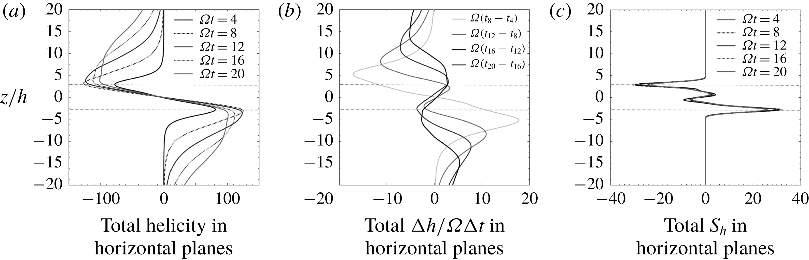
The evolution of the horizontally averaged values of
 $h$
,
 $\unicode[STIX]{x2202}h/\unicode[STIX]{x2202}t$
and
 $S_{h}$
for
 $Ro=0.01$
,
 $Ek=0.0023$
and
 $\unicode[STIX]{x1D6FA}t=4{-}20$
.
The buoyancy field,
 $-\unicode[STIX]{x1D717}$
(a), helicity (b) and helicity source,
 $S_{h}$
(c), for a layer of buoyant blobs, each viewed in the horizontal planes,
 $z/\unicode[STIX]{x1D6FF}=-2.8,0,2.8$
.
 $Ro=0.01$
,
 $Ek=0.0023$
and
 $\unicode[STIX]{x1D6FA}t=12$
.

The corresponding horizontally averaged values of
 $h$
,
 $\unicode[STIX]{x2202}h/\unicode[STIX]{x2202}t$
and
 $S_{h}$
are shown in figure 11 as a function of
 $z$
, with
 $-40<z/\unicode[STIX]{x1D6FF}<40$
and
 $\unicode[STIX]{x2202}h/\unicode[STIX]{x2202}t$
estimated as
 $\unicode[STIX]{x0394}h/\unicode[STIX]{x0394}t$
. This shows the evolution of
 $h$
,
 $\unicode[STIX]{x2202}h/\unicode[STIX]{x2202}t$
and
 $S_{h}$
over a range of times,
 $\unicode[STIX]{x1D6FA}t=4{-}20$
. As with the Gaussian blob, the magnitude of the helicity at the top and bottom of the cloud eventually saturates. Also, as the helicity propagates away from the cloud at the group velocity of low-frequency inertial waves, the spatial extent of the source remains more or less constant, which is a consequence of the low value of
 $Ro$
. (At low
 $Ro$
there is very little advection of the buoyancy field.) Finally note that, while
 $h$
is well correlated with
 $S_{h}$
within the buoyant slab, there is no corresponding correlation between
 $\unicode[STIX]{x2202}h/\unicode[STIX]{x2202}t$
and
 $S_{h}$
at large times, consistent with what we observed for a single buoyant blob.
We note in passing that it would be interesting to compare these helicity distributions with those predicted by the reduced (quasi-geostrophic) model of Calkins, Julien & Marti (Reference Calkins, Julien and Marti2013), which offers the possibility of a more efficient computation of low
 $Ro$
dynamics.
Finally, figure 12 shows the corresponding spatial distributions of
 $-\unicode[STIX]{x1D717}$
(a), helicity (b), and helicity source,
 $S_{h}$
(c), in the three horizontal planes
 $z/\unicode[STIX]{x1D6FF}=-2.8,0,2.8$
. While the detailed distributions of
 $h$
and
 $S_{h}$
are highly intermittent, the statistically asymmetric distribution about
 $z=0$
is clear.
4.2 Rossby number of order unity
In some planetary dynamo simulations the value of
 $Ro$
corresponding to the small-scale structures is not that much less than unity, perhaps
 $Ro\sim 0.1$
. In order to determine the sensitivity of our results to
 $Ro$
, we now consider a case in which
 $Ro$
is of order unity. Figures 13–16 show the results where the initial Rossby number is set to
 $Ro=\unicode[STIX]{x1D717}_{0}g/2\unicode[STIX]{x1D6FA}^{2}\unicode[STIX]{x1D6FF}=1$
. All other parameters remain unchanged. Figure 13 shows snapshots of (a)
 $-\unicode[STIX]{x1D717}$
, (b)
 $u_{z}$
and (c)
 $h$
, all at
 $\unicode[STIX]{x1D6FA}t=12$
and all in the
 $x$
–
 $z$
plane. Rather remarkably, despite the much higher value of
 $Ro$
, the wave field looks very similar to the low
 $Ro$
case. The main difference between figures 9 and 13 is that there is now significant advection of the buoyancy by the wave field, which causes some mixing of
 $\unicode[STIX]{x1D717}$
. This, in turn, causes the characteristic transverse length scale to increase as a result of cross-diffusion of the buoyancy field, growing by a factor of
 ${\sim}3$
by
 $\unicode[STIX]{x1D6FA}t=12$
. The growth in this length scale results in the effective value of
 $Ro$
falling from unity at
 $t=0$
to
 ${\sim}0.3$
at
 $\unicode[STIX]{x1D6FA}t=12$
.
A horizontal layer of buoyant blobs provides the initial condition for a simulation with
 $Ro=1$
and
 $Ek=0.0023$
. (a) The buoyancy field
 $-\unicode[STIX]{x1D717}$
, (b)
 $u_{z}$
and (c)
 $h$
, all in the
 $x$
–
 $z$
plane and at time
 $\unicode[STIX]{x1D6FA}t=12$
.

The horizontal movement of the
 $\unicode[STIX]{x1D717}$
-field leads to the observed inclination of the columnar eddies which, in principle, is similar to the trailing Taylor columns observed by Hide, Ibbetson & Lighthill (Reference Hide, Ibbetson and Lighthill1968). The corresponding distributions of the helicity source terms,
 $S_{1}$
,
 $S_{2}$
and
 $S_{h}=S_{1}+S_{2}$
, averaged in
 $y$
, are shown in figure 14, again in the
 $x$
–
 $z$
plane and for
 $\unicode[STIX]{x1D6FA}t=12$
. In this case all three source terms are predominantly negative at the top of the buoyant cloud and positive at the bottom. There is also a marked oscillation in
 $S_{2}$
, although not in
 $S_{h}$
, which is less evident (though still detectable) in the low
 $Ro$
case.
The horizontally averaged values of
 $h$
,
 $\unicode[STIX]{x2202}h/\unicode[STIX]{x2202}t$
and
 $S_{h}$
are shown in figure 15 as a function of
 $z$
, with
 $-40<z/\unicode[STIX]{x1D6FF}<40$
. This shows the evolution of
 $h$
,
 $\unicode[STIX]{x2202}h/\unicode[STIX]{x2202}t$
and
 $S_{h}$
over a range of times,
 $\unicode[STIX]{x1D6FA}t=4{-}20$
. Unlike the low
 $Ro$
case, the magnitude of the helicity at the top and bottom of the cloud does not saturate, almost certainly because the r.m.s. buoyancy field declines throughout the simulation as a result of the mixing-induced cross-diffusion of
 $\unicode[STIX]{x1D717}$
. Nevertheless, we see the usual spatial correlation in the signs of the horizontally averaged values of
 $h$
and
 $S_{h}$
.
The helicity sources in a horizontal layer of buoyant blobs: (a)
 $S_{1}$
, (b)
 $S_{2}$
and (c)
 $S_{h}=S_{1}+S_{2}$
, all averaged in
 $y$
and shown in the
 $x$
–
 $z$
plane.
 $Ro=1$
,
 $Ek=0.0023$
and
 $\unicode[STIX]{x1D6FA}t=12$
.

The evolution of the horizontally averaged values of
 $h$
,
 $\unicode[STIX]{x2202}h/\unicode[STIX]{x2202}t$
and
 $S_{h}$
for
 $Ro=1$
,
 $Ek=0.0023$
,
 $\unicode[STIX]{x1D6FA}t=4{-}20$
.

Finally, figure 16 shows the distribution of
 $-\unicode[STIX]{x1D717}$
(a), helicity (b) and helicity source,
 $S_{h}$
(c), in the three horizontal planes
 $z/\unicode[STIX]{x1D6FF}=-2.8,0,2.8$
. As in figure 12, the distributions of
 $h$
and
 $S_{h}$
are complicated, but the statistically asymmetric distribution about
 $z=0$
is clear. The main effect of increasing
 $Ro$
is that the
 $\unicode[STIX]{x1D717}$
field is smoother (less spotty) and has a larger transverse length scale, almost certainly as a result of the mixing of the buoyancy by the wave-induced velocity field, and by the enhanced diffusion that ensues. It is also notable that there is now significant anisotropy in the
 $x$
–
 $y$
plane, with
 $S_{h}$
adopting a streaky structure with the streaks aligned with
 $\boldsymbol{g}$
.
The buoyancy field,
 $-\unicode[STIX]{x1D717}$
(a), helicity (b) and helicity source,
 $S_{h}$
(c), for a layer of buoyant blobs, each viewed in the horizontal planes
 $z/\unicode[STIX]{x1D6FF}=-2.8,0,2.8$
.
 $Ro=1$
,
 $Ek=0.0023$
and
 $\unicode[STIX]{x1D6FA}t=12$
.

5 Discussion: implications for numerical dynamos and planetary cores
So far we have ignored the presence of boundaries, which are of course important for the dynamics in a planetary core. The first point to note is that low-frequency inertial wave packets travelling along the rotation axis will reflect at the mantle, reversing their group velocity and helicity in the process (Greenspan Reference Greenspan1968). In the absence of dissipation, this produces standing waves, which are of course Taylor columns. The helicity in a Taylor column is zero, and so the mechanism of helicity segregation described here will be effective in a planetary core only if there is significant dissipation. That is to say, in order to avoid the perfect cancellation of helicity in the reflected and incident waves, we require that waves launched in the interior be somewhat dissipated before they reach the mantle. Since the Ekman number is tiny in the core of the Earth, this dissipation can only be ohmic in nature. In principle, the magnitude of the ohmic dissipation can be estimated, but the calculation is very sensitive to the assumed magnitude of the magnetic field, which is a poorly constrained parameter, and to the size of the smallest scales in the core, which is unknown. So the question of dissipation remains an open one.
A second difficulty arises from the fact that, although the simulations exhibit a statistical bias in the concentration of buoyant anomalies towards the equatorial regions, in practice the fluctuations in density are everywhere. So buoyant anomalies which are closer to the mantle than the equator will emit waves whose helicity in the interior is opposite in sign to that of the waves which were launched close to the equator. Once again, there will be a tendency for cancellation in helicity, and so the segregation mechanism proposed here will be effective only if the statistical inhomogeneity in buoyancy sources is strong enough.
A third weakness of the inertial wave model for establishing planetary helicity distributions is that the magnetic field within a planet will modify the inertial waves, forming hybrid magnetic–Coriolis waves. This process is discussed in, for example, Bardsley & Davidson (Reference Bardsley and Davidson2016, Reference Bardsley and Davidson2017), where it is noted that the main effect of the magnetic field is to reduce the magnitude of the group velocity. However, such hybrid waves still carry negative helicity northward and positive helicity to the south, just like inertial waves.
Given the three caveats above, perhaps the strongest argument in favour of helicity segregation by inertial waves is the simplicity of (2.18). Perhaps it is worth taking a closer look at this equation. Rearranging the terms in the inviscid helicity equation (2.10), we find that, without approximation,
 $$\begin{eqnarray}\frac{\unicode[STIX]{x2202}}{\unicode[STIX]{x2202}t}(\boldsymbol{u}\boldsymbol{\cdot }\unicode[STIX]{x1D74E})=-\unicode[STIX]{x1D735}\boldsymbol{\cdot }\boldsymbol{F}+S_{2},\quad \boldsymbol{F}=-(2\boldsymbol{u}^{2})\unicode[STIX]{x1D734}-\boldsymbol{u}\times \frac{\unicode[STIX]{x2202}\boldsymbol{u}}{\unicode[STIX]{x2202}t}.\end{eqnarray}$$
Now
 $$\begin{eqnarray}\boldsymbol{u}\times \frac{\unicode[STIX]{x2202}\boldsymbol{u}}{\unicode[STIX]{x2202}t}<2\unicode[STIX]{x1D734}\boldsymbol{u}^{2},\end{eqnarray}$$
since the highest frequency for inertial waves is
 $2\unicode[STIX]{x1D6FA}$
. It follows that
 $\boldsymbol{F}=-(2\boldsymbol{u}^{2})\unicode[STIX]{x1D734}$
is always the larger of the two contributions to the wave flux. Moreover
 $$\begin{eqnarray}\unicode[STIX]{x1D735}\boldsymbol{\cdot }\left(\boldsymbol{u}\times \frac{\unicode[STIX]{x2202}\boldsymbol{u}}{\unicode[STIX]{x2202}t}\right)=\unicode[STIX]{x1D74E}\boldsymbol{\cdot }\frac{\unicode[STIX]{x2202}\boldsymbol{u}}{\unicode[STIX]{x2202}t}-\boldsymbol{u}\boldsymbol{\cdot }\frac{\unicode[STIX]{x2202}\unicode[STIX]{x1D74E}}{\unicode[STIX]{x2202}t},\end{eqnarray}$$
and so we may drop the term
 $\boldsymbol{u}\times \unicode[STIX]{x2202}\boldsymbol{u}/\unicode[STIX]{x2202}t$
altogether in one of two situations:
(i) the helicity is being carried by low-frequency wave packets,
$\unicode[STIX]{x1D71B}\ll |\unicode[STIX]{x1D734}|$
, as in equation (2.18);(ii) we have maximal helicity in the waves, with the velocity and vorticity fields proportional,
$\unicode[STIX]{x1D74E}=\mp k\boldsymbol{u}$
, as in a monochromatic inertial wave and as observed in inertial wave packets by Davidson & Ranjan (Reference Davidson and Ranjan2015).


In either of these situations we have the approximation
 $$\begin{eqnarray}\frac{\unicode[STIX]{x2202}}{\unicode[STIX]{x2202}t}(\boldsymbol{u}\boldsymbol{\cdot }\unicode[STIX]{x1D74E})\approx \unicode[STIX]{x1D735}\boldsymbol{\cdot }[(2\boldsymbol{u}^{2})\unicode[STIX]{x1D734}]+2\boldsymbol{g}\boldsymbol{\cdot }(\boldsymbol{u}\times \unicode[STIX]{x1D735}\unicode[STIX]{x1D717}).\end{eqnarray}$$
Let us integrate this over a cylindrical annulus,
 $V_{N}$
, lying outside the tangent cylinder, of radial extent
 $\unicode[STIX]{x0394}s$
, and bounded above by the mantle and below by the equator
 $$\begin{eqnarray}\frac{\text{d}}{\text{d}t}\int _{V_{N}}\boldsymbol{u}\boldsymbol{\cdot }\unicode[STIX]{x1D74E}\,\text{d}V=-2\unicode[STIX]{x1D6FA}\left\{\int _{equator}\boldsymbol{u}^{2}\,\text{d}A-\int _{mantle}\boldsymbol{u}^{2}\,\text{d}A\right\}+\int _{V_{N}}S_{2}\,\text{d}V.\end{eqnarray}$$
Similarly, for the corresponding annulus in the south,
 $V_{S}$
, which is bounded below by the mantle and above by the equator, we have
 $$\begin{eqnarray}\frac{\text{d}}{\text{d}t}\int _{V_{S}}\boldsymbol{u}\boldsymbol{\cdot }\unicode[STIX]{x1D74E}\,\text{d}V=2\unicode[STIX]{x1D6FA}\left\{\int _{equator}\boldsymbol{u}^{2}\,\text{d}A-\int _{mantle}\boldsymbol{u}^{2}\,\text{d}A\right\}+\int _{V_{S}}S_{2}\,\text{d}V,\end{eqnarray}$$
where
 $\boldsymbol{u}$
in (5.5) and (5.6) is the fluctuating velocity. Now it is difficult to predict what the integral of
 $S_{2}$
will be, as can be seen by comparing figures 10(b) and 14(b). Moreover, we have omitted all dissipative and magnetic effects in these equations. Nevertheless, it seems that a relatively large fluctuating kinetic energy in the equatorial regions will favour the north–south asymmetry in the azimuthally averaged helicity shown in figures 1(c) and 2(a), and this applies to inertial waves of all frequencies. Of course, physically this reflects the fact that, if we have more wave activity near the equator than the mantle, then waves will tend to disperse away from the equatorial regions, carrying with them helicity of the observed signs.
6 Conclusions
The strong spatial correlation between the distribution of
 $h$
and of
 $S_{h}$
in the dynamo simulations tends to suggest an in situ generation of helicity in dynamo simulations, rather than the dispersal of helicity by waves, as previously argued by the authors. However, the observation that there is no such correlation between
 $\unicode[STIX]{x2202}h/\unicode[STIX]{x2202}t$
and
 $S_{h}$
argues against such an in situ generation mechanism. Either way, the correlation, or lack of correlation, between
 $h$
,
 $\unicode[STIX]{x2202}h/\unicode[STIX]{x2202}t$
and
 $S_{h}$
needs to be explained.
We have offered an explanation for the paradoxical observation that
 $h$
and
 $S_{h}$
are strongly correlated, yet there is no such correlation between
 $\unicode[STIX]{x2202}h/\unicode[STIX]{x2202}t$
and
 $S_{h}$
, by showing that inertial waves interact with the buoyancy field in such a way as to induce a source
 $S_{h}$
which adopts the same sign as the helicity in the local wave flux. Moreover, we have confirmed that, in simple model problems, the sign of
 $h$
is simply determined by the direction of the wave flux. We conclude that the observed distributions of
 $h$
and
 $S_{h}$
in the numerical dynamos are consistent with the transport of helicity by waves.
Acknowledgements
The authors thank P. K. Yeung of Georgia Tech for sharing his DNS code and U. Christensen and J. Wicht for many interesting discussion on core dynamics and for sharing their dynamo data set. The authors also thank the Leverhulme Trust for their generous support through the grant RPG-2015-195/RG77943.