1 Introduction
Over the past few decades, due to the vast number of applications in coating technology, liquid film flows have received much attention. Many experimental and theoretical works have focused on a liquid film flowing down a flat plane (Oron, Davis & Bankoff Reference Oron, Davis and Bankoff1997; Craster & Matar Reference Craster and Matar2009) and a cylindrical surface (Quéré Reference Quéré1999). A liquid film coating a cylindrical surface has potential applications in oil recovery and biological flows, particularly in connection with the drawing of fibres from liquid baths. The well-known Plateau–Rayleigh mechanism modulated by the gravity-driven flow gives rise to many interesting dynamical phenomena, e.g. organized sliding beads and the breakup of liquid films, which have attracted much experimental and theoretical attention (De Ryck & Quéré Reference De Ryck and Quéré1996; Duprat et al. Reference Duprat, Ruyer-Quil, Kalliadasis and Giorgiutti-Dauphiné2007; Ruyer-Quil et al. Reference Ruyer-Quil, Treveleyan, Giorgiutti-Dauphiné and Kalliadasis2008; Duprat et al. Reference Duprat, Giorgiutti-Dauphiné, Tseluiko, Saprykin and Kalliadasis2009).
To investigate the dynamics of a liquid film coating the exterior surface of a vertical fibre at low Reynolds number, most theoretical works have employed a reduced-order model. Pioneering work on a very thin film was carried out by Frenkel (Reference Frenkel1992), who derived a thin film model and showed that the liquid film is linearly unstable due to azimuthal curvature. The nonlinear dynamics of the thin film model has been examined to account for droplet formation by Kalliadasis & Chang (Reference Kalliadasis and Chang1994) and Chang & Demekhin (Reference Chang and Demekhin1999). Kliakhandler, Davis & Bankhoff (Reference Kliakhandler, Davis and Bankhoff2001) investigated a much thicker film, where the thin film model can no longer be applied, and observed three different flow regimes, labelled ‘a’, ‘b’ and ‘c’. In flow regime ‘a’, where the flow rate is high
 $({\sim}22~\text{mm}^{3}~\text{s}^{-1})$
, large droplets maintain their shape, travel at a constant speed and are separated by a flat film. At moderate flow rates
 $({\sim}11~\text{mm}^{3}~\text{s}^{-1})$
, flow regime ‘b’ labels a necklace-like structure, i.e. close and regularly spaced droplets. Flow regime ‘c’ corresponds to an oscillatory state observed at low flow rates (
 ${\sim}5~\text{mm}^{3}~\text{s}^{-1}$
), in which a big droplet coexists with several small beads. The large droplet catches up with and consumes small beads at its front, before breaking up into small beads at its rear. The thick film model retaining the full surface curvature proposed by Kliakhandler et al. (Reference Kliakhandler, Davis and Bankhoff2001) failed to find a solution similar to flow regime ‘a’ in numerical simulations. Craster & Matar (Reference Craster and Matar2006) reduced the curvature asymptotically and showed that the travelling wave solutions of the asymptotic model capture the correct wave speed of flow regime ‘a’. Neither the thick film model nor the asymptotic model, however, capture the wave speed of the necklace-like structure in flow regime ‘b’. This perhaps is because the long-wave assumption of the reduced-order models does not hold in flow regime ‘b’. The flow regime ‘c’ is not steady but oscillates due to the droplet coalescence and breakup process. Recent experimental studies of flow regime ‘c’ have confirmed that it is a time-periodic state (Sadeghpour, Zeng & Ju Reference Sadeghpour, Zeng and Ju2017; Zeng et al.
Reference Zeng, Sadeghpour, Warrier and Ju2017). In most previous studies, steady travelling wave solutions have been computed and compared with the flow regime ‘c’ (Craster & Matar Reference Craster and Matar2006; Ruyer-Quil et al.
Reference Ruyer-Quil, Treveleyan, Giorgiutti-Dauphiné and Kalliadasis2008; Novbari & Oron Reference Novbari and Oron2009). However, it is questionable whether or not a travelling wave solution should be used to compare with the oscillating flow regime ‘c’, when one is steady and the other is unsteady. It is natural to ask whether there is an unsteady solution, i.e. a relative periodic orbit solution, that can capture not only the dynamics of the oscillation, but also the wave speed of flow regime ‘c’.
When inertial effects are taken into account, two coupled equations governing the film thickness and the flow rate can be derived, such as the integral boundary layer model (Trifonov Reference Trifonov1992; Sisoev et al. Reference Sisoev, Craster, Matar and Gerasimov2006; Shkadov, Beloglazkin & Gerasimov Reference Shkadov, Beloglazkin and Gerasimov2008), the energy integral model (Novbari & Oron Reference Novbari and Oron2009) and the weighted residual model (Ruyer-Quil et al. Reference Ruyer-Quil, Treveleyan, Giorgiutti-Dauphiné and Kalliadasis2008). A shortcoming of the integral boundary layer model is that it fails to predict the correct linear stability of a film flowing down a moderately tilted plane, which can be addressed by the weighted residual model (Ruyer-Quil & Manneville Reference Ruyer-Quil and Manneville1998). The energy integral model and the weighted residual model are more accurate than the thick film model and the asymptotic model. For instance, a small capillary ripple in front of the big droplet predicted by the asymptotic model is not obvious in experiment, but is eliminated in the weighted residual model (Ruyer-Quil et al. Reference Ruyer-Quil, Treveleyan, Giorgiutti-Dauphiné and Kalliadasis2008). Pradas, Tseluiko & Kalliadasis (Reference Pradas, Tseluiko and Kalliadasis2011), however, have shown that this small capillary ripple can have an important effect on the formation of bound states, which consist of several different sized pulses moving together. The bound states can be either steady or oscillatory (Pradas et al. Reference Pradas, Tseluiko and Kalliadasis2011). Very recently, Blyth et al. (Reference Blyth, Tseluiko, Lin and Kalliadasis2018) showed that there are countably infinite sets of bound states in an electrified liquid film flowing down an inclined plane.
For industrial applications, it is interesting to design an active control method to modify the interfacial instability to induce pattern formation. The application of an electric field has been a successful candidate for this purpose (Papageorgiou Reference Papageorgiou2018), e.g. using an electric field to control pattern formation in a liquid film on a flat plane (Schäffer et al. Reference Schäffer, Thurn-Albrecht, Russell and Steiner2000; Craster & Matar Reference Craster and Matar2005) and droplet production from liquid jets (Conroy et al. Reference Conroy, Matar, Craster and Papageorgiou2011; Wang & Papageorgiou Reference Wang and Papageorgiou2011). The idea of using an electric field was also transplanted into the control of instability of liquid film flows on vertical fibres (Wray, Matar & Papageorgiou Reference Wray, Matar and Papageorgiou2012; Wray, Papageorgiou & Matar Reference Wray, Papageorgiou and Matar2013a ,Reference Wray, Papageorgiou and Matar b ; Ding et al. Reference Ding, Xie, Wong and Liu2014; Liu, Chen & Ding Reference Liu, Chen and Ding2018). The asymptotic model was used to investigate the dynamics of the electrified films (Wray et al. Reference Wray, Matar and Papageorgiou2012, Reference Wray, Papageorgiou and Matar2013a ,Reference Wray, Papageorgiou and Matar b ; Ding et al. Reference Ding, Xie, Wong and Liu2014; Liu et al. Reference Liu, Chen and Ding2018). Recently, other control methods, e.g. varying the nozzle size (Sadeghpour et al. Reference Sadeghpour, Zeng and Ju2017) or using a countercurrent gas flow (Zeng et al. Reference Zeng, Sadeghpour, Warrier and Ju2017), have been used to modulate the pattern formation in liquid films on vertical fibres.
When the liquid is a leaky dielectric, the electric field can suppress the Plateau–Rayleigh instability or attract the liquid to the electrode, leading to the ‘touchdown’ structure (Wray et al.
Reference Wray, Matar and Papageorgiou2012, Reference Wray, Papageorgiou and Matar2013a
,Reference Wray, Papageorgiou and Matar
b
), where the liquid interface is attracted to the fibre (the inner electrode). When the liquid is perfectly conducting, instead, a spike-like structure is observed (Ding et al.
Reference Ding, Xie, Wong and Liu2014; Liu et al.
Reference Liu, Chen and Ding2018), where the liquid interface touches the outer electrode. Self-similarity analysis has shown that the minimal film thickness in the touchdown state scales as
 $(\unicode[STIX]{x0394}t)^{1/3}$
(Wray et al.
Reference Wray, Papageorgiou and Matar2013a
), and the spike-like structure develops as
 $(\unicode[STIX]{x0394}t)^{1/6}$
(where
 $\unicode[STIX]{x0394}t=t_{s}-t$
with singularity formation time
 $t_{s}$
) (Liu et al.
Reference Liu, Chen and Ding2018). The interested reader may consult the review paper by Saville (Reference Saville1997) for more details on the dielectric models of liquids. When the electric field was not strong, both a saturated travelling wave state and an oscillatory state were observed in these studies. The oscillation can either be periodic or chaotic in the presence of an electric field. Further, oscillation between large droplets that are close in size can occur.
Oscillatory behaviour is different in non-electrified film flow (Ding et al. Reference Ding, Xie, Wong and Liu2014), where oscillations occur only through the interaction between a large droplet and a much smaller droplet. The travelling wave solution for a single droplet shows that a large droplet moves faster than a small droplet, and therefore a conclusion of the theoretical study is that a big droplet catches up with, and consumes, a smaller droplet. The resulting bigger droplet can be unstable, breaking up into smaller droplets, leading to an oscillatory or chaotic state (Craster & Matar Reference Craster and Matar2006; Ding & Wong Reference Ding and Wong2017). Travelling wave solutions of a non-electrified film flow of slightly different sized droplets can move as a bound state (Trifonov Reference Trifonov1992; Ruyer-Quil & Manneville Reference Ruyer-Quil and Manneville1998; Sisoev et al. Reference Sisoev, Craster, Matar and Gerasimov2006), which do not exhibit oscillation. Moreover, experimental study of a non-electrified film has also shown that slightly different sized droplets can also move in a stable bound state (Duprat et al. Reference Duprat, Ruyer-Quil, Kalliadasis and Giorgiutti-Dauphiné2007). These theoretical and experimental studies imply that oscillation is unlikely to occur through the interactions between large droplets, without the help of an electric field. A minor point to address, however, is that it is not clear how the electric field induces the oscillation between large droplets in the electrified film flow on a vertical cylinder. A related question is how the oscillation influences the wave speed. Does the oscillation accelerate or slow down the motion of droplets? A quick answer to this question can be found in figure 4(b–d), where in general it is seen that the oscillation slows down the droplet.
Travelling wave solutions cannot provide a full understanding of the dynamics of a liquid film flowing down a vertical cylinder, in particular, the oscillatory phenomenon. From the viewpoint of dynamical systems theory, travelling wave solutions are called ‘relative’ equilibria of the phase space. Their integral properties are constant and do not capture the dynamics of unsteady flows. Travelling waves, however, can be unstable to a Hopf bifurcation, leading to the emergence of relative periodic orbits (Cvitanović, Davidchack & Siminos Reference Cvitanović, Davidchack and Sminos2010; Chantry, Willis & Kerswell Reference Chantry, Willis and Kerswell2014). These ‘relative’ periodic orbits are periodic orbits in a frame with non-zero phase speed. (A periodic orbit of the original system must have exactly zero phase shift after one period, but the probability of such a shift is zero for a homogeneous system, unless the solution carries a reflectional symmetry.) Indeed, relative period orbits are thought of as the building blocks of a chaotic attractor in turbulent flows, e.g. turbulent Couette flow (Viswanath Reference Viswanath2007), Kolmogorov flow (Chandler & Kerswell Reference Chandler and Kerswell2013) and pipe flow (Budanur et al. Reference Budanur, Short, Farazmand and Willis2017). This paper is therefore inspired by recent research in transitional turbulence. We aim to explore relative periodic solutions in liquid film flows down a vertical fibre. In contrast to steady travelling wave solutions, we believe that relative periodic solutions should provide a better understanding of the oscillatory dynamics of the electrified film, and, in particular, the regime ‘c’ of non-electrified flow.
A synopsis of this paper is as follows. In § 2 we formulate the problem and derive a long-wave model. Numerical methods for extracting steady travelling wave and relative periodic solutions are provided in § 3. The oscillation caused by an electric field is discussed in § 4.1, which is followed by a discussion of oscillation in a non-electrified film in § 4.2. A conclusion is presented in § 5.
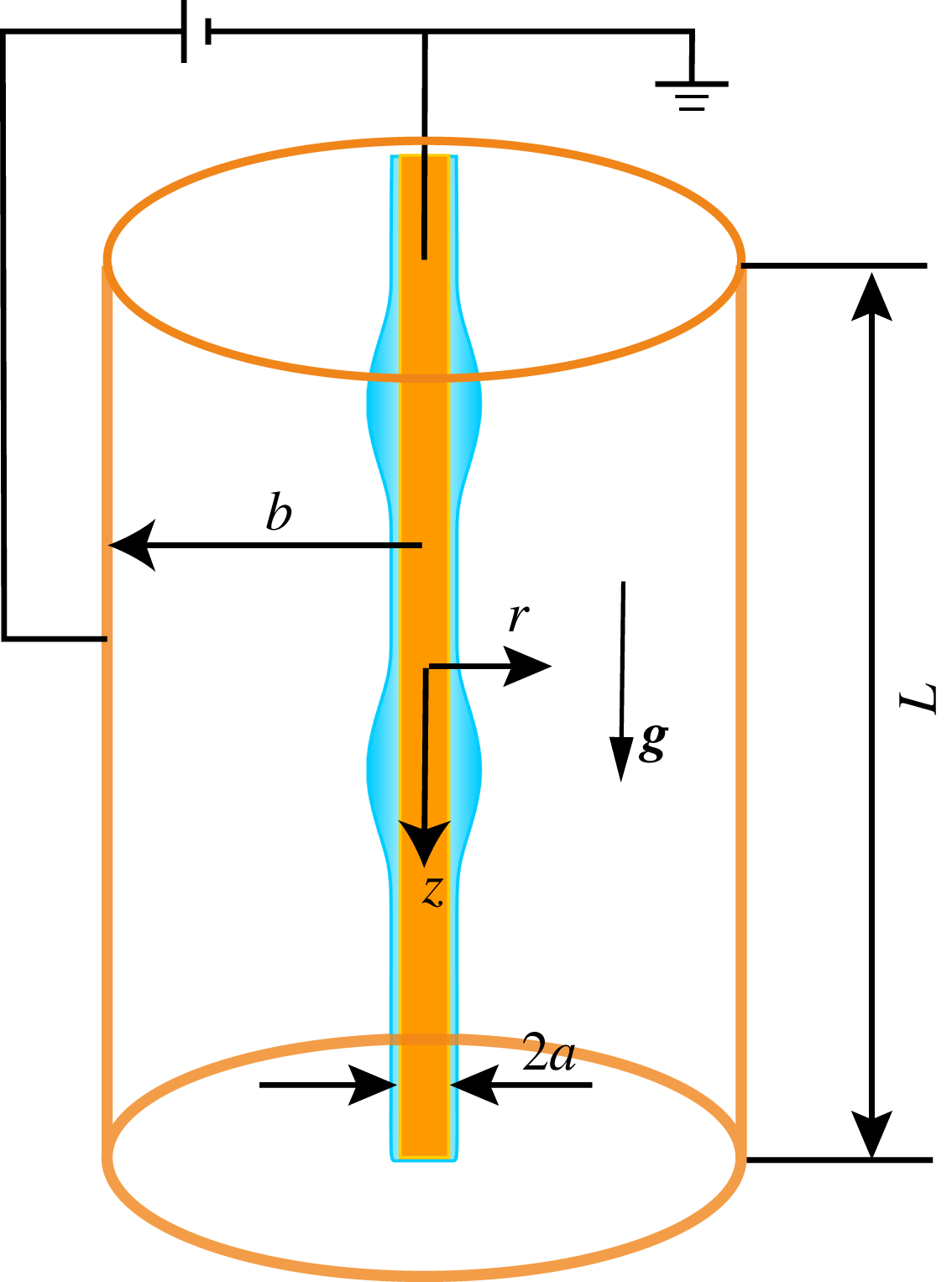
Geometry of the system. The mean radius of the liquid film is
 $h_{0}$
.

2 Mathematical formulation
We consider an axisymmetric perfectly conducting liquid film of constant density
 $\unicode[STIX]{x1D70C}$
and dynamic viscosity
 $\unicode[STIX]{x1D707}$
. The flow down a vertical fibre, modelled by a cylinder, is driven by gravity
 $g$
and subjected to a radial electric field (see figure 1). The annular flow system is enclosed in a coaxial cylindrical electrode. A high electric voltage
 $\unicode[STIX]{x1D719}_{0}$
is applied at the outer electrode, while the central metal fibre is grounded. Throughout this paper, the surrounding dielectric gas is considered to be inviscid and its dynamics is therefore neglected. The outer cylinder cannot be neglected, however, as it is required to impose a uniform electric field.
We assume that the mean radius to the surface of the fluid ring
 $h_{0}$
is much smaller than its characteristic length
 $\mathscr{L}$
in the axial direction and define a small parameter
 $\unicode[STIX]{x1D716}=h_{0}/\mathscr{L}$
. Craster & Matar (Reference Craster and Matar2006) took the length scale
 $\mathscr{L}$
to be related to the capillary length,
 $\mathscr{L}=\unicode[STIX]{x1D6FE}/\unicode[STIX]{x1D70C}gh_{0}$
, so that the dimensionless equations would not rely on the fluid thickness being small relative to the fibre radius, but instead small relative to a dynamic length scale. The small parameter is then
 $\unicode[STIX]{x1D716}=\unicode[STIX]{x1D70C}gh_{0}^{2}/\unicode[STIX]{x1D6FE}$
, which is also known as the Bond number
 $Bo$
, and in experiment is typically small,
 $Bo\sim 0.3$
or so (Craster & Matar Reference Craster and Matar2006). We non-dimensionalize the system by introducing the length scales
 $r=h_{0}r^{\prime }$
and
 $z=\mathscr{L}z^{\prime }$
, pressure scale
 $p-p_{g}=\unicode[STIX]{x1D70C}g\mathscr{L}p^{\prime }$
, electric potential
 $\unicode[STIX]{x1D719}=\unicode[STIX]{x1D719}_{0}$
, velocity scales
 $w=Ww^{\prime }$
and
 $u=\unicode[STIX]{x1D716}Wu^{\prime }$
, and time
 $t=\mathscr{L}/Wt^{\prime }$
(with
 $W=\unicode[STIX]{x1D70C}h_{0}^{2}g/\unicode[STIX]{x1D707}$
, and
 $p_{g}$
is the pressure of the gas phase). This paper considers the leading-order dynamics, and the evolution equation of the interfacial shape
 $h(z,t)$
derived by Ding et al. (Reference Ding, Xie, Wong and Liu2014) is adopted:
 $$\begin{eqnarray}h_{t}+\frac{1}{h}\left[\frac{1-p_{z}}{4}\left(h^{4}\ln \left(\frac{h}{\unicode[STIX]{x1D6FC}}\right)+\frac{(\unicode[STIX]{x1D6FC}^{2}-h^{2})(3h^{2}-\unicode[STIX]{x1D6FC}^{2})}{4}\right)\right]_{z}=0,\end{eqnarray}$$
where
 $p=-E_{b}\unicode[STIX]{x1D719}_{r}^{2}/2+1/h-\unicode[STIX]{x1D716}^{2}h_{zz}$
and the electrostatic force
 $\unicode[STIX]{x1D719}_{r}^{2}=h^{-2}[\ln (h/\unicode[STIX]{x1D6FD})]^{-2}$
at the leading-order approximation. The dimensionless radii are
 $\unicode[STIX]{x1D6FC}=a/h_{0}$
and
 $\unicode[STIX]{x1D6FD}=b/h_{0}$
;
 $E_{b}=\unicode[STIX]{x1D716}\unicode[STIX]{x1D700}\unicode[STIX]{x1D719}_{0}^{2}/\unicode[STIX]{x1D70C}gh_{0}^{3}$
is the electric Weber number; and
 $\unicode[STIX]{x1D700}$
is the electric permittivity. When the electric field is turned off, (2.1) reduces to the model of Craster & Matar (Reference Craster and Matar2006) immediately.
In this paper, to seek the recurrent solutions, i.e. relative equilibria (travelling waves) and relative periodic orbits, we solve for the local cross-sectional area
 $S=h^{2}$
rather than the liquid radius
 $h$
:
 $$\begin{eqnarray}S_{t}+2\left((1-p_{z})\left[\frac{S^{2}}{4}\ln \left(\frac{S^{1/2}}{\unicode[STIX]{x1D6FC}}\right)+\frac{(3S-\unicode[STIX]{x1D6FC}^{2})(\unicode[STIX]{x1D6FC}^{2}-S)}{16}\right]\right)_{z}=0,\end{eqnarray}$$
where
 $$\begin{eqnarray}p=\frac{1}{S^{1/2}}-\unicode[STIX]{x1D716}^{2}\left(\frac{1}{2}S^{-1/2}S_{zz}-\frac{1}{4}S^{-3/2}S_{z}^{2}\right)-\frac{E_{b}}{2}S^{-1}\left(\frac{1}{2}\ln S-\ln \unicode[STIX]{x1D6FD}\right)^{-2}.\end{eqnarray}$$
It follows from mass conservation that
 $S$
is temporally conserved:
 $$\begin{eqnarray}\langle S\rangle =\frac{1}{L}\int _{0}^{L}S\,\text{d}z=1,\end{eqnarray}$$
where
 $L$
is the axial length of the domain. The equations for
 $S$
are numerically more convenient than those for
 $h$
: when using a Newton method to update
 $S$
, where
 $S$
is expressed as a Fourier expansion, the mean mode is fixed by the constraint (2.4), while changes to the coefficients of the other modes do not affect (2.4).
For visualization purposes, we introduce an energy-like norm
 $\mathscr{E}=\langle S^{2}/2\rangle$
. Then, the energy balance in the system is
 $$\begin{eqnarray}\dot{\mathscr{E}}={\mathcal{I}}-{\mathcal{D}},\end{eqnarray}$$
where
 $$\begin{eqnarray}\displaystyle {\mathcal{I}} & = & \displaystyle {\textstyle \frac{1}{2}}\langle S^{-3/2}S_{z}^{2}Q\rangle ,\end{eqnarray}$$
 $$\begin{eqnarray}\displaystyle {\mathcal{D}} & = & \displaystyle \langle \unicode[STIX]{x1D716}^{2}({\textstyle \frac{1}{2}}S^{-1/2}S_{z}S_{zzz}+{\textstyle \frac{3}{8}}S^{-5/2}S_{z}^{4}-{\textstyle \frac{3}{4}}S^{-3/2}S_{zz}S_{z}^{2})Q\rangle \nonumber\\ \displaystyle & & \displaystyle +\,\langle E_{b}/2(S^{-1}({\textstyle \frac{1}{2}}\ln S-\ln \unicode[STIX]{x1D6FD})^{-2})_{z}S_{z}Q\rangle ,\end{eqnarray}$$
with
 $Q=S^{2}\ln (S^{1/2}/\unicode[STIX]{x1D6FC})/4+(3S-\unicode[STIX]{x1D6FC}^{2})(\unicode[STIX]{x1D6FC}^{2}-S)/16$
. We will project the solution onto the energy production
 ${\mathcal{I}}$
and energy dissipation
 ${\mathcal{D}}$
plane. For travelling waves (TWs), the dissipation equals the production
 ${\mathcal{D}}={\mathcal{I}}$
; and for relative periodic orbits (RPOs), the orbits in the
 ${\mathcal{I}}$
versus
 ${\mathcal{D}}$
plane are closed loops with a temporal average centred on
 ${\mathcal{D}}={\mathcal{I}}$
.
3 Recurrent solutions: dynamical systems approach
Recurrent solutions of the dynamical system (2.2) satisfy
 $$\begin{eqnarray}S(z+l,t+T)=S(z,t),\end{eqnarray}$$
where
 $l$
is a spatial shift along the axis of the fibre and
 $T$
is a period. Each RPO has its particular period
 $T$
, while for a TW the period
 $T$
may be freely chosen, and the shift is related to the phase speed by
 $c=l/T$
. If
 $T$
is large, then we may need to account for the periodicity,
 $c=(l+nL)/T$
, where
 $n$
is an integer. For an RPO solution, we use
 $\bar{c}$
to represent its mean speed.
The solution of (2.2) is approximated by a Fourier expansion:
 $$\begin{eqnarray}S(z,t)=\mathop{\sum }_{j=-N+1}^{N}{\hat{S}}_{j}(t)\exp \left(\text{i}\,j\frac{2\unicode[STIX]{x03C0}}{L}z\right).\end{eqnarray}$$
Derivatives in
 $z$
are computed in the Fourier space, and nonlinear terms are evaluated on a uniform grid in real space. For the calculations of this paper, we have used 256–320 Fourier modes. An implicit Gear’s method in time is implemented, and the error after
 $T/\unicode[STIX]{x0394}t$
time steps of size
 $\unicode[STIX]{x0394}t$
is less than
 $10^{-6}$
relative to the solution for
 $\unicode[STIX]{x0394}t\rightarrow 0$
(Ding et al.
Reference Ding, Xie, Wong and Liu2014).
Given an initial guess
 $(S_{0},l,T)$
, using Newton’s method to find a root of
 $(S-S_{0})$
, where
 $S=S(z+l,t+T)$
and
 $S_{0}=S(z,t)$
, a better guess
 $(S_{0}+\unicode[STIX]{x1D6FF}S_{0},l+\unicode[STIX]{x1D6FF}l,T+\unicode[STIX]{x1D6FF}T)$
is given by
 $$\begin{eqnarray}\frac{\unicode[STIX]{x2202}S}{\unicode[STIX]{x2202}S_{0}}\unicode[STIX]{x1D6FF}S_{0}+\frac{\unicode[STIX]{x2202}S}{\unicode[STIX]{x2202}l}\unicode[STIX]{x1D6FF}l+\frac{\unicode[STIX]{x2202}S}{\unicode[STIX]{x2202}T}\unicode[STIX]{x1D6FF}T-\unicode[STIX]{x1D6FF}S_{0}=-(S-S_{0}).\end{eqnarray}$$
As there are
 $2N+2$
unknowns
 $\unicode[STIX]{x1D6FF}S_{0}$
,
 $\unicode[STIX]{x1D6FF}l$
and
 $\unicode[STIX]{x1D6FF}T$
, we need two more constraints to close the system. We impose that
 $\unicode[STIX]{x1D6FF}S_{0}$
has no component that shifts the solution in the
 $z$
direction or the
 $t$
direction (Viswanath Reference Viswanath2007),
 $$\begin{eqnarray}\displaystyle & \displaystyle \unicode[STIX]{x1D6FF}S_{0}\frac{\unicode[STIX]{x2202}S_{0}}{\unicode[STIX]{x2202}z}=0, & \displaystyle\end{eqnarray}$$
 $$\begin{eqnarray}\displaystyle & \displaystyle \unicode[STIX]{x1D6FF}S_{0}\frac{\unicode[STIX]{x2202}S_{0}}{\unicode[STIX]{x2202}t}=0. & \displaystyle\end{eqnarray}$$
For TWs we drop the second condition in (3.5) and we take
 $T$
fixed. Equations (3.3), (3.4) and (3.5) constitute the following system:
 $$\begin{eqnarray}\mathscr{A}\boldsymbol{x}=\boldsymbol{b},\end{eqnarray}$$
where
 $\boldsymbol{x}=(\unicode[STIX]{x1D6FF}S_{0},\unicode[STIX]{x1D6FF}l,\unicode[STIX]{x1D6FF}T)$
and
 $\boldsymbol{b}=(S-S_{0},0,0)$
. The system (3.6) can be solved using the GMRES method, which approximates the solution in the Krylov subspace spanned by
 ${\mathcal{K}}_{m}=\{\boldsymbol{b},\mathscr{A}\boldsymbol{b},\mathscr{A}^{2}\boldsymbol{b},\ldots ,\mathscr{A}^{m-1}\boldsymbol{b}\}$
. Typically
 ${\mathcal{K}}_{m}$
is small,
 $m=O(10)$
. To evaluate the result of multiplication by the Jacobian, we use the approximation
 $$\begin{eqnarray}\frac{\unicode[STIX]{x2202}S}{\unicode[STIX]{x2202}S_{0}}\unicode[STIX]{x1D6FF}S_{0}\approx \frac{S(z,T;S_{0}+e\,\unicode[STIX]{x1D6FF}S_{0})-S(z,T;S_{0})}{e},\end{eqnarray}$$
wherein
 $e$
is an empirical small parameter. We set
 $e$
such that
 $e\,\Vert \unicode[STIX]{x1D6FF}S_{0}\Vert /\Vert S_{0}\Vert =10^{-4}$
. We terminate the GMRES iterations when
 $\Vert \mathscr{A}\boldsymbol{x}-\boldsymbol{b}\Vert /\Vert \boldsymbol{b}\Vert \leqslant 10^{-3}$
. For the Newton step, the iteration is terminated when
 $\Vert S-S_{0}\Vert /\Vert S_{0}\Vert <10^{-6}$
and typically the relative error is
 $O(10^{-8})$
for the solutions presented in this paper. Failure of the Newton method is commonplace when the initial guess is not good enough. To improve the domain of convergence, we applied a ‘hook-step’ to move
 $(\unicode[STIX]{x1D6FF}S_{0},\unicode[STIX]{x1D6FF}l,\unicode[STIX]{x1D6FF}T)$
within a trust region. For more information on the numerical method, excellent descriptions of the Newton–Krylov hook-step method can be found in Viswanath (Reference Viswanath2007) and Chandler & Kerswell (Reference Chandler and Kerswell2013). The Newton–Krylov code is validated by recomputing the TW solutions by a direct Newton code of Ding et al. (Reference Ding, Xie, Wong and Liu2014) (see figure 4).
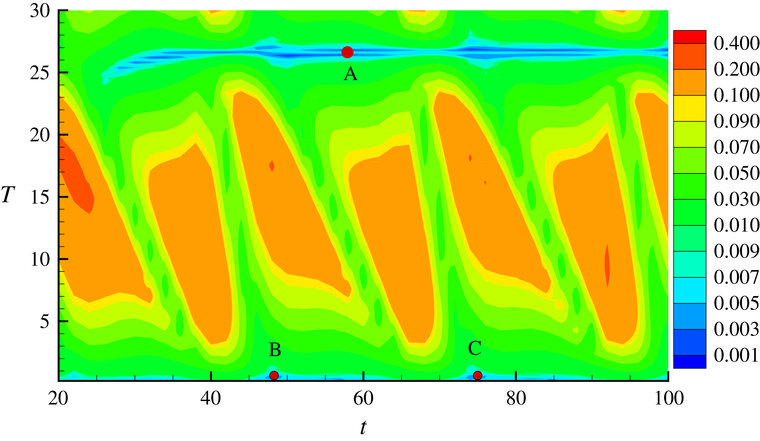
Example of
 $R_{d}(t,T)$
at
 $E_{b}=2$
and
 $L=4$
contoured over
 $t\in [20,100]$
and
 $T\in [0.2,30]$
. The minimal value of
 $R_{d}\sim 10^{-3}$
is found near
 $T=26$
. The three marked points, labelled A, B and C, are used as initial guesses for the Newton–Krylov iteration, and only point A converges.

A good initial guess for the Newton–Krylov code is required in order to stand a good chance of convergence to a solution. In this paper, we follow Cvitanović & Gibson (Reference Cvitanović and Gibson2010) and search for near recurrences by calculating the normalized difference between states, namely
 $R_{d}(t,T)$
, which is minimized over a continuous shift in
 $z$
direction, after each interval of
 $t=0.1$
or
 $t=0.2$
:
 $$\begin{eqnarray}R_{d}(t,T)=\min _{0\leqslant l\leqslant L}\frac{\Vert S(t+T,z+l)-S(t,z)\Vert }{\Vert S(t,z)\Vert }.\end{eqnarray}$$
We consider cases where
 $R_{d}<10^{-2}$
as candidates. Figure 2 illustrates a good initial guess at around
 $40<t<100$
with
 $T\approx 26$
. A snapshot of
 $S(z,t)$
taken from ‘A’ was used as an initial guess and converged to an RPO discussed in § 4.1. Once an RPO is obtained, we used parametric continuation to track solutions.
4 Results and discussion
In the following discussions, we first explore RPOs in an electrified film in § 4.1, which aims at providing insight into the oscillation caused by interactions between two big droplets. When the electric field is turned off, however, interactions between big droplets do not cause an oscillatory flow. Instead, oscillation is due to the complicated interaction between a large droplet and a much smaller droplet. And we will demonstrate that this oscillation caused by a large droplet and a small droplet can be represented by an RPO in § 4.2. In particular, the flow regime ‘c’ in the experimental study (Kliakhandler et al. Reference Kliakhandler, Davis and Bankhoff2001) is compared with an RPO solution.
4.1 Invariant solutions in an electrified film
This section examines the oscillatory phenomenon in an electrified film. Previous numerical simulations have shown that an oscillation between big droplets can occur when subjected to an electric field (Wray et al.
Reference Wray, Papageorgiou and Matar2013a
; Ding et al.
Reference Ding, Xie, Wong and Liu2014). Stability analysis of a uniform film,
 $S=1$
, has shown that for
 $\unicode[STIX]{x1D6FD}<\exp (1)$
the electric field can enhance the linear instability. For
 $\unicode[STIX]{x1D6FD}>\exp (1)$
, however, the electric field impedes the linear instability, but is destabilizing with respect to finite-amplitude perturbations. The flow then proceeds to the formation of an oscillatory state or spike-like singular state, dependent on the value of
 $\unicode[STIX]{x1D6FD}$
(Ding et al.
Reference Ding, Xie, Wong and Liu2014). In this paper, we are interested in the oscillatory state and therefore fix the radius of the outer electrode at
 $\unicode[STIX]{x1D6FD}=\exp (1.1)$
. In the following discussion, we fix the small parameter
 $\unicode[STIX]{x1D716}$
, and the radius of the fibre
 $\unicode[STIX]{x1D6FC}$
at
 $(\unicode[STIX]{x1D716},\unicode[STIX]{x1D6FC})=(0.2,0.25)$
following previous studies, (e.g. Craster & Matar Reference Craster and Matar2006; Liu et al.
Reference Liu, Chen and Ding2018). To understand the oscillation dynamics between big droplets, we consider a periodic computational domain that is large enough for two big droplets. To determine an appropriate domain size
 $L$
, we refer to the linear stability analysis by Ding et al. (Reference Ding, Xie, Wong and Liu2014), where the wavelength of the most unstable mode in the electrified film is
 $$\begin{eqnarray}\frac{2\sqrt{2}\,\unicode[STIX]{x1D716}\unicode[STIX]{x03C0}}{\displaystyle \sqrt{1+\frac{E_{b}(1-\ln (\unicode[STIX]{x1D6FD}))}{\ln ^{3}(\unicode[STIX]{x1D6FD})}}}\sim 2.\end{eqnarray}$$
We therefore start with domain sizes of
 $L\sim 4$
for
 $0\leqslant E_{b}\leqslant 4$
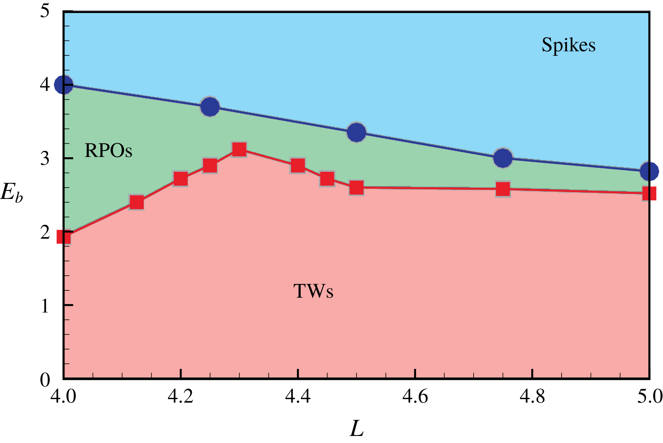
to allow two big droplets. Figure 3 shows the type of solution observed in simulations for the range
 $4\leqslant L\leqslant 5$
. For
 $L>6$
, we expect three or more big droplets to form in the domain.
Phase diagram of solution regimes in the
 $L$
versus
 $E_{b}$
plane. The boundaries separating different solution regimes are obtained starting from RPOs and tracking where they undergo transition to spikes or TWs.

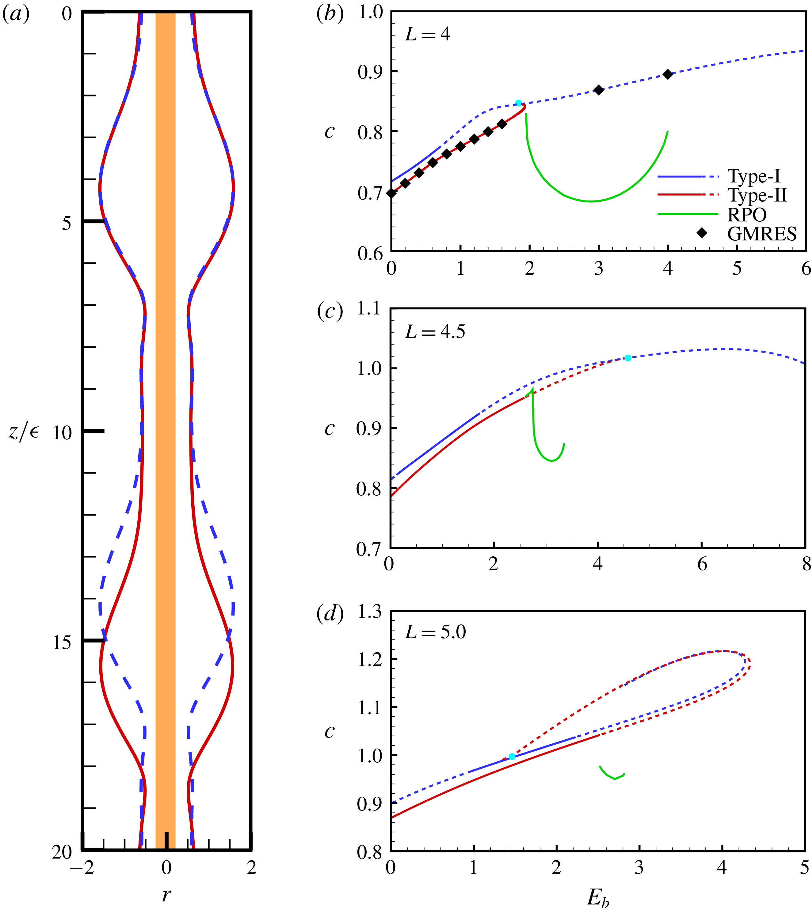
(a) The profiles of the ‘two different/identical droplets’ (type I/type II) illustrated by ‘blue/red’ lines for
 $E_{b}=1$
,
 $L=4$
. (b–d) The wave speed
 $c$
versus the electric number
 $E_{b}$
for
 $L=4$
, 4.5 and 5, respectively. The type-I TW branch for
 $L=5$
stops at
 $E_{b}=2.76$
after it turns back, as the singular structure appears. Curves for TWs are obtained by a direct Newton–Raphson iteration using the code of Ding et al. (Reference Ding, Xie, Wong and Liu2014). Curves for RPOs in (b–d) are obtained from the Newton–Krylov method implemented in this work. Stable/unstable TW branches are solid/dashed lines. The Newton–Krylov method is validated by reproducing the TW solution as marked by diamonds in (b). The bullets indicate where the type-II TW connects with type-I TW.

Initially, to find stable states in simulations, we perturb the trivial solution
 $S=1$
by harmonic waves
 $$\begin{eqnarray}S(z,0)=1+0.1\cos \left(n\frac{2\unicode[STIX]{x03C0}}{L}z\right),\end{eqnarray}$$
with
 $n=1$
or
 $n=2$
and with
 $E_{b}$
small. For
 $L=4$
, we find that the system evolves into one of two stable TW states. For
 $n=2$
, two identical droplets form, hereafter called type I. Their spatial period is
 $L/2$
, but they are stable to small disturbances of
 $n=1$
type. Starting with
 $n=1$
in (4.2), two slightly different droplets form, hereafter referred to as type II. The two forms of TW solution are illustrated in figure 4(a). Starting from these non-oscillatory solutions at
 $L=4$
,
 $E_{b}=0$
, pseudo-arclength continuation with the code of Ding et al. (Reference Ding, Xie, Wong and Liu2014) has been used to track the TW solutions and the wave speed
 $c$
against the electric Weber number
 $E_{b}$
, shown in figure 4(b–d). For the case of type-II TW, the
 $c$
versus
 $E_{b}$
curve is shown in figure 4(b), which folds back at
 $E_{b}\approx 1.94$
for
 $L=4$
, while the curve stops at around
 $E_{b}=4.3$
for
 $L=4.5$
. Thus, for both
 $L=4$
and
 $L=4.5$
this indicates that the type-II TWs do not exist when the electric field exceeds some critical value. For
 $L=5$
neither type of solution exists for
 $E_{b}\gtrsim 4$
.
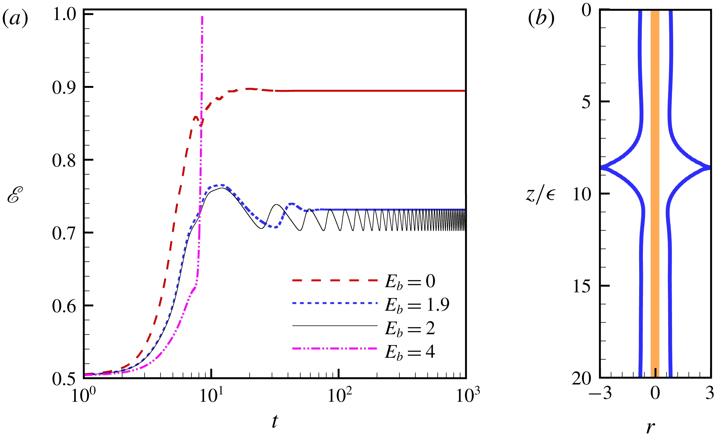
(a) Evolution of the energy norm
 $\mathscr{E}=\langle S^{2}/2\rangle$
at different electric number subject to the initial condition
 $S(z,0)=1+0.1\cos (\unicode[STIX]{x03C0}z/2)$
where
 $z\in [0,4]$
. For
 $E_{b}=0,1.9$
, steady type-II TWs are obtained (see that
 $\mathscr{E}$
becomes invariant). (b) The spike-like structure plotted at
 $t\approx 8.5$
at
 $E_{b}=4$
,
 $L=4$
.

Numerical simulations of TW solutions show that they lose stability to an oscillatory bound state when
 $E_{b}$
exceeds a critical value (see figure 5
a). The oscillation suggests the existence of RPOs, which will be discussed presently. For larger
 $E_{b}$
, we observe that two droplets start to merge, and the minimal gap between the liquid interface and outer electrode reduces quickly – Ding et al. (Reference Ding, Xie, Wong and Liu2014) showed that the outer electrode attracts the interface, and the liquid interface becomes unstable. It is quickly attracted to the outer electrode when the gap is small, leading to the formation of the spike-like structure. (An example of the spike-like structure can be found in figure 5
b.) It is natural to examine whether the oscillatory solutions are linked to the TW solutions through oscillatory bifurcations.
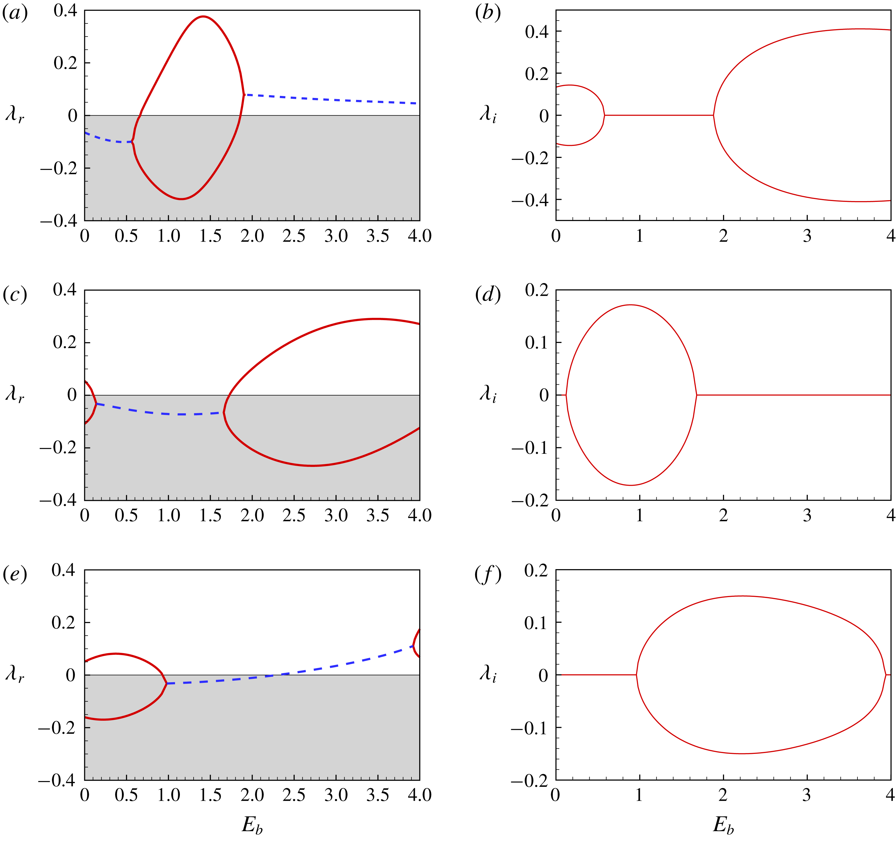
The two leading eigenvalues (either two real or a complex pair) of the type-I TWs are plotted against
 $E_{b}$
in figure 6 for (a,b)
 $L=4$
, (c,d)
 $L=4.5$
and (e,f)
 $L=5$
. The eigenvalues for the type-II TW for these parameters are shown in figure 7.
Eigenvalue of the type-I TWs versus the electric number
 $E_{b}$
at (a,b)
 $L=4$
, (c,d)
 $L=4.5$
and (e,f)
 $L=5$
. The red solid (blue dashed) lines represent the stationary (oscillatory) mode. For
 $L=5$
, the stability of the lower branch of type-I TW is investigated in (e,f).

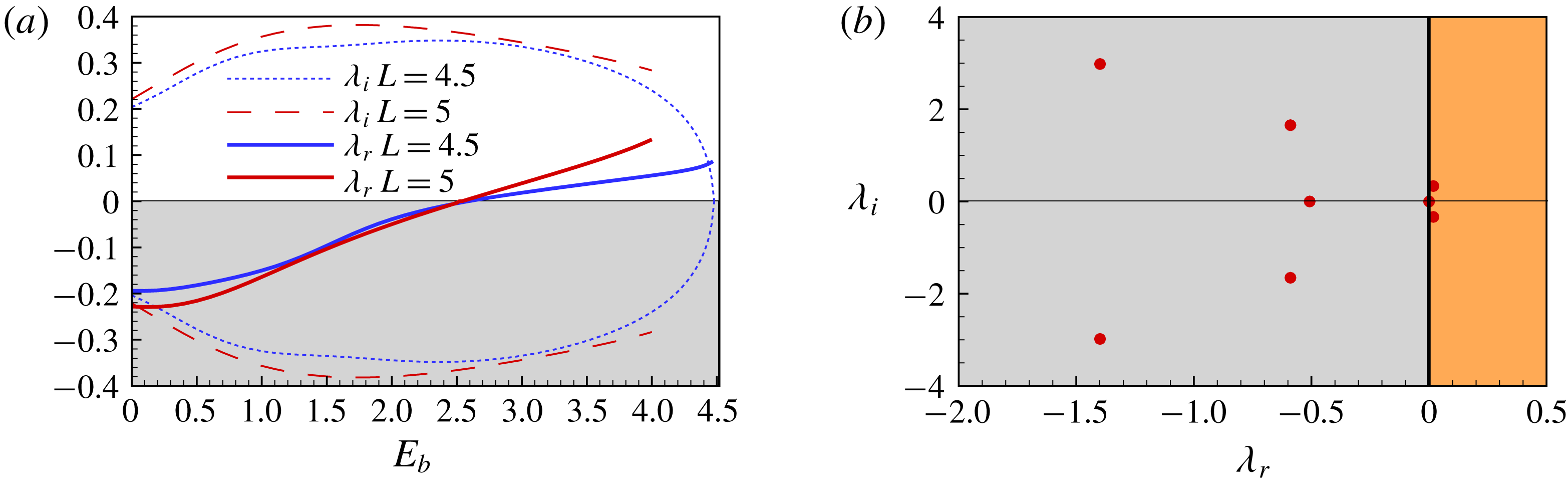
(a) Leading eigenvalue for type-II TWs versus the electric number
 $E_{b}$
at
 $L=4.5$
and 5. The leading mode is oscillatory. (b) The spectra of the eigenvalue problem of type-II TW at
 $E_{b}=3$
,
 $L=4.5$
; two unstable eigenvalues were detected.

At
 $L=4$
the type-I TW becomes unstable when
 $E_{b}>0.66$
, but the unstable mode is not oscillatory until
 $E_{b}\gtrsim 1.94$
. Numerical simulation shows that type-I TWs lose stability and evolve into type-II TWs for
 $0.66<E_{b}<1.94$
, and the type-II TWs are stable over this range. For
 $E_{b}>1.94$
the dynamics develop into an RPO.
For
 $L=4.5$
, figure 6(c,d) shows that the oscillatory eigenmode is always stable, and the unstable mode is always real. In this case, RPOs do not originate from the instability of type-I TWs, but instead come from the instability of type-II TWs when
 $E_{b}>2.6$
, as demonstrated by figure 7(a). Figure 4(c) shows that the RPO branch connects with the type-II TW branch.
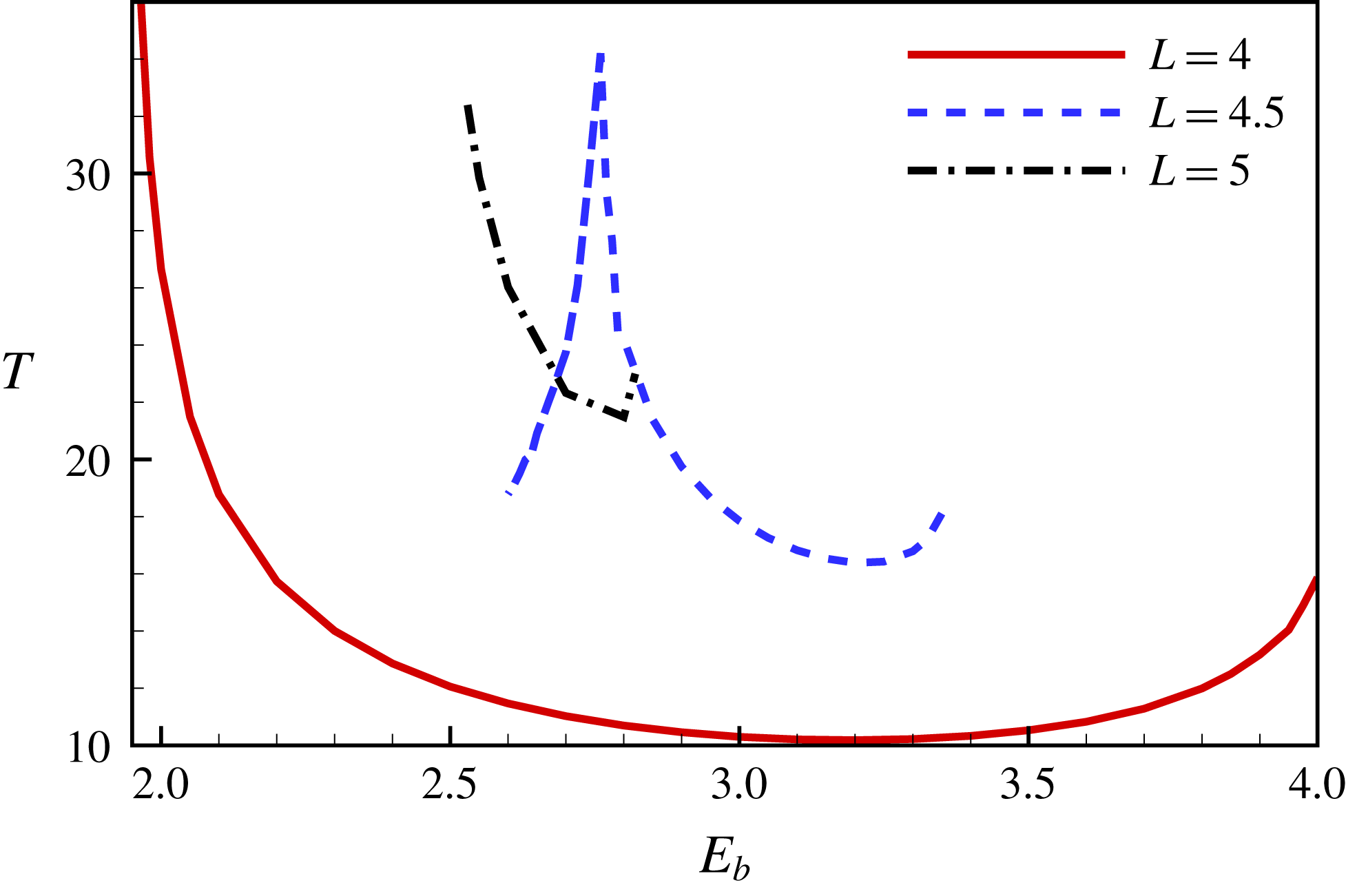
The periods of RPOs versus the electric Weber number at different domain sizes
 $L=4$
, 4.5 and 5.

For
 $L=5$
, type-I TWs are unstable to a real mode when
 $E_{b}<0.92$
or
 $E_{b}>3.92$
, while the mode is unstable and oscillatory for
 $2.23<E_{b}<3.92$
. It should be stressed that the type-II TW is a stable attractor when
 $2.23<E_{b}<2.52$
at
 $L=5$
and numerical simulation confirms that type-II TWs rather than RPOs are observed in this range. For type-II TWs, figure 7(a,b) shows that the type-II TWs become unstable to an oscillatory mode for
 $E_{b}>2.52$
. Hence, for
 $L=5$
, RPOs may be born from the instability of either type-I or type-II TWs for
 $E_{b}>2.52$
.
For the
 $E_{b}$
values where there are oscillations, time series of the energy norm
 $\mathscr{E}$
are found to be periodic, implying the existence of RPOs. Using a snapshot of
 $S(z,t_{0})$
at some
 $t_{0}$
from the numerical simulations as the initial guess for our Newton–Krylov code, an exact RPO solution can be obtained. Typical profiles of the RPOs at
 $L=4$
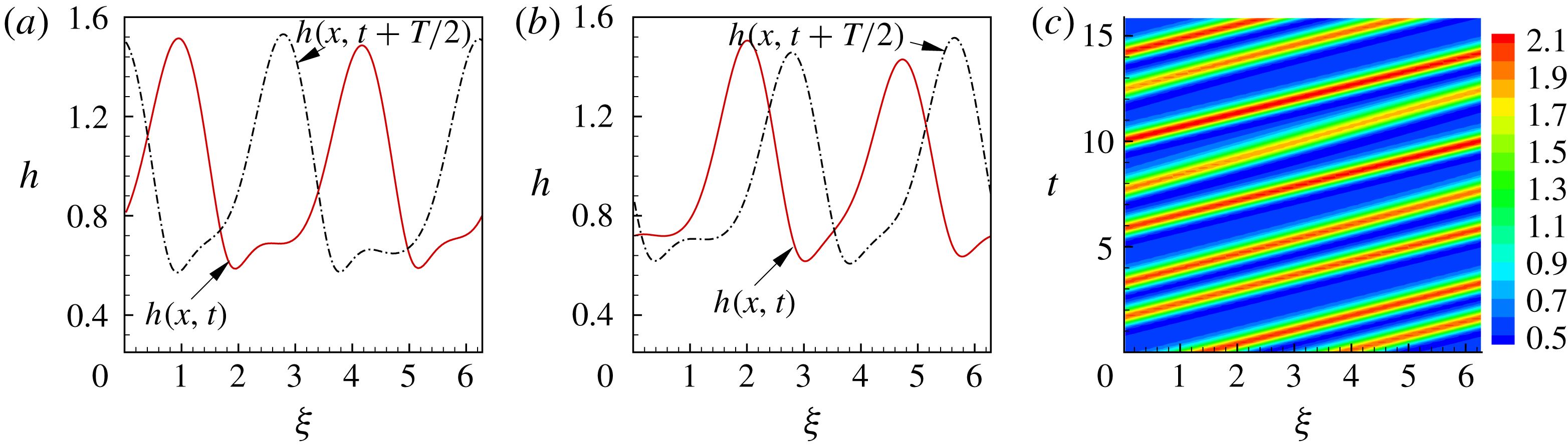
are shown in figure 9(a,b). A spatio-temporal diagram of the film radius
 $h$
in figure 9(c) illustrates the oscillating behaviour for two different sized droplets. A more clear picture of the oscillation can be seen in our supplementary movie (available at https://doi.org/10.1017/jfm.2019.450). The dynamics of the RPOs is projected into the
 ${\mathcal{I}}-{\mathcal{D}}$
versus
 ${\mathcal{D}}$
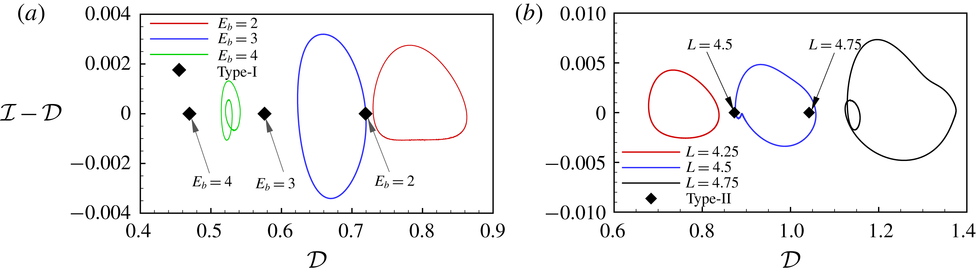
plane in figure 10(a). TWs are fixed points on the horizon axis
 ${\mathcal{I}}={\mathcal{D}}$
, while RPOs are closed loops that cross this axis. For
 $L=4$
, using a parametric continuation method, RPOs are found for
 $E_{b}$
up to
 $E_{b}\approx 4$
. Further increase in
 $E_{b}$
leads to the formation of the spike-like structure. When the length of the computational domain is increased for fixed
 $E_{b}=3$
, RPOs are found up to around
 $L=4.75$
, shown in figure 10(b). Further increasing
 $L$
also leads to formation of the spike-like structure.
(a,b) The interfacial profiles at times
 $t$
,
 $t+T/2$
and
 $t+T$
. The electric number and time period in (a) and (b) are respectively
 $(E_{b}=2,T=26.6521,l=0.4520)$
and
 $(E_{b}=3,T=10.2997,l=-0.9633)$
. (c) The space–temporal diagram of
 $h(x,t)$
in a period at
 $E_{b}=4$
. Here, the coordinate
 $\unicode[STIX]{x1D709}=(2\unicode[STIX]{x03C0}/L)z$
and
 $L=4$
.

RPOs in the
 ${\mathcal{I}}-{\mathcal{D}}$
versus
 ${\mathcal{D}}$
plane at (a)
 $L=4$
and (b)
 $E_{b}=3$
. Diamonds are steady TW solutions.

The period of the RPOs,
 $T$
, is plotted against the electric Weber number
 $E_{b}$
in figure 8(a). The electric field has dual effects on the oscillation. For
 $L=4,5$
, the oscillation becomes faster (
 $T$
decreases) as
 $E_{b}$
increases initially. However, beyond some critical point, the oscillation becomes slower (
 $T$
increases). For
 $L=4.5$
, the dynamics is a bit more complicated. The oscillation becomes slower (
 $T$
increases) as
 $E_{b}$
increases from the bifurcation point
 $E_{b}\approx 2.6$
. Then, the oscillation becomes faster (
 $T$
decreases) as
 $E_{b}>2.78$
. However, as
 $E_{b}$
increases further, the oscillation becomes slower (
 $T$
increases). Referring to figure 4(b–d), the RPO runs faster/slower when the oscillation is slower/faster. The RPO is slower than the type-I TW, which might be faster than type-II TW (see figures 4
c and 15
b).
For
 $L=4$
, as
 $E_{b}$
is reduced towards
 $1.94$
, we find that
 $T\rightarrow \infty$
and our Newton–GMRES code stops converging, due to the breakdown of the linearization (3.7) for large
 $T$
. We are able to get to sufficiently large
 $T$
, however, to identify that the RPO connects to the type-I TW. The divergence of
 $T$
is in agreement with the linear stability analysis where
 $\unicode[STIX]{x1D706}_{i}\rightarrow 0$
as
 $E_{b}\rightarrow 1.94^{+}$
(figure 6
b). For
 $L=4.5$
, a Hopf bifurcation occurs at
 $E_{b}\approx 2.6$
for the type-II TW (figure 7
a). The eigenvalue at the bifurcation point
 $E_{b}=2.6$
predicts a period
 $T=2\unicode[STIX]{x03C0}/\unicode[STIX]{x1D706}_{i}=2\unicode[STIX]{x03C0}/0.34\approx 18.48$
. The RPO branch is quite contorted as it approaches the type-II branch, but at the last points computed on the branch the period of the RPO is
 ${\approx}18.70$
and decreasing, in good agreement with the linear stability calculation. For
 $L=5$
, we have been unable to identify a connection between the RPO and the TWs (see figure 4
d), as far as we are able to reliably perform the calculations.
To summarize the results in this section, the solution regimes are constructed in figure 3, and, in particular, the oscillatory bound states are represented by RPOs. We have demonstrated that the two large droplets cannot survive in a steady bound state but can do so in an oscillatory bound state when
 $E_{b}$
exceeds a critical value (e.g.
 $E_{b}=2$
and see figure 5
a). This indicates that we may expect to see steady travelling waves, relative periodic solutions or spike-like structures in experimental study, depending on the strength of the electric field and droplet spacing. When the electric field is weak, we should observe the formation of a steady liquid viscous bead train due to the Rayleigh–Plateau mechanism. The steady wave train will lose stability and an oscillating state will emerge as the strength of the electric field increases. The spike-like structure should appear when the electric field is strong.
4.2 Invariant solutions in a non-electrified film
In the absence of an electric field, it is observed that droplets can move in either a stable or an unstable bound state (Duprat et al. Reference Duprat, Ruyer-Quil, Kalliadasis and Giorgiutti-Dauphiné2007), but this oscillation is different from that discussed in § 4.1 – here, experimental and numerical studies have shown that the oscillation is caused by the interaction between a large droplet and a much smaller droplet (Craster & Matar Reference Craster and Matar2006; Duprat et al. Reference Duprat, Ruyer-Quil, Kalliadasis and Giorgiutti-Dauphiné2007). The large droplet eats small droplets, and can then break up into small droplets. Such a process is cyclical, and we will demonstrate that it can be represented by RPOs.
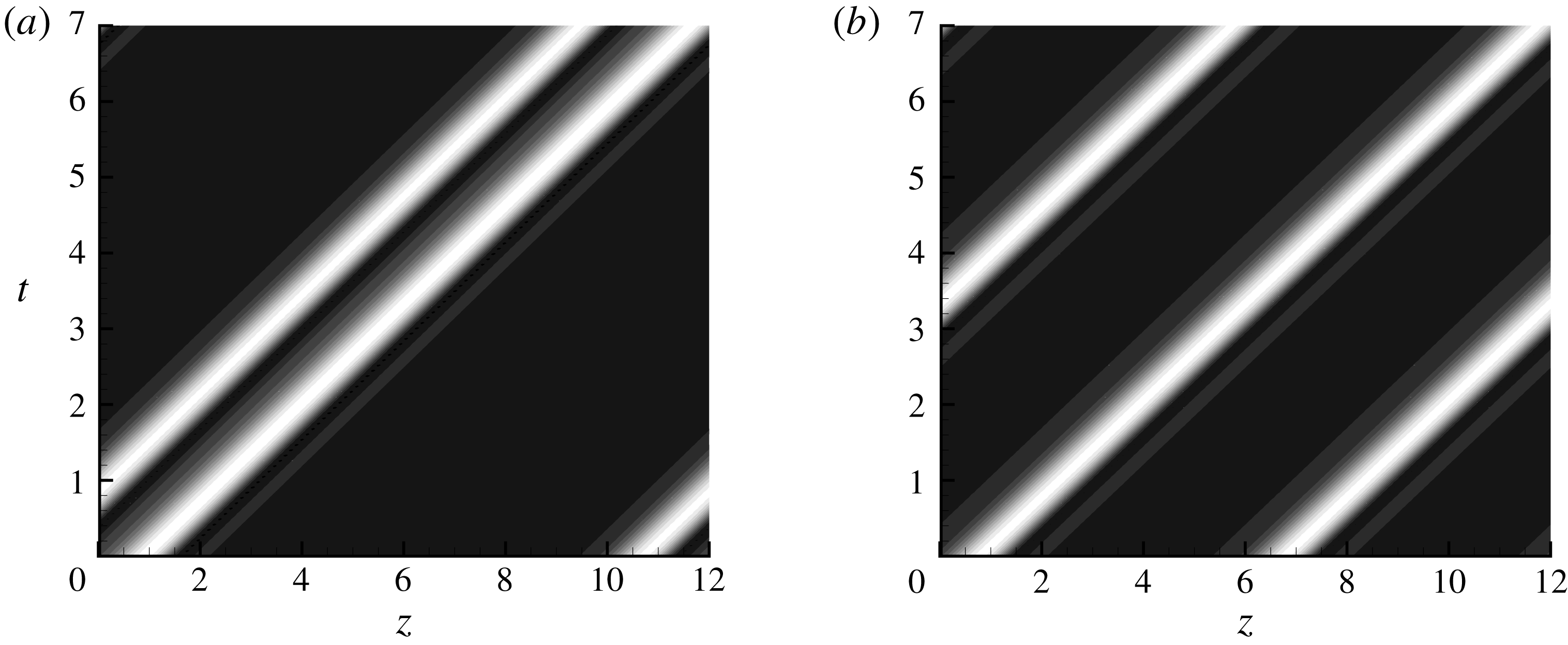
The space–time diagram for type-II TW (a), and type-I TW (b). The bright (dark) shading indicates elevated (depressed) regions. The dependent parameters are
 $Bo=\unicode[STIX]{x1D716}=0.2$
,
 $\unicode[STIX]{x1D6FC}=0.25$
and
 $L=12$
.

Space–time diagrams at
 $L=12$
are shown in figure 11. In fact, for
 $L=12$
, other types of solutions do exist, e.g. a one-droplet solution, a three-droplet solution, and so on. The multi-droplet solutions can be stable or unstable bound states. Here we only consider two big droplets in the computational domain so as to isolate the oscillation dynamics. The leading eigenvalues of type-I and type-II TWs are tracked against the domain size
 $L$
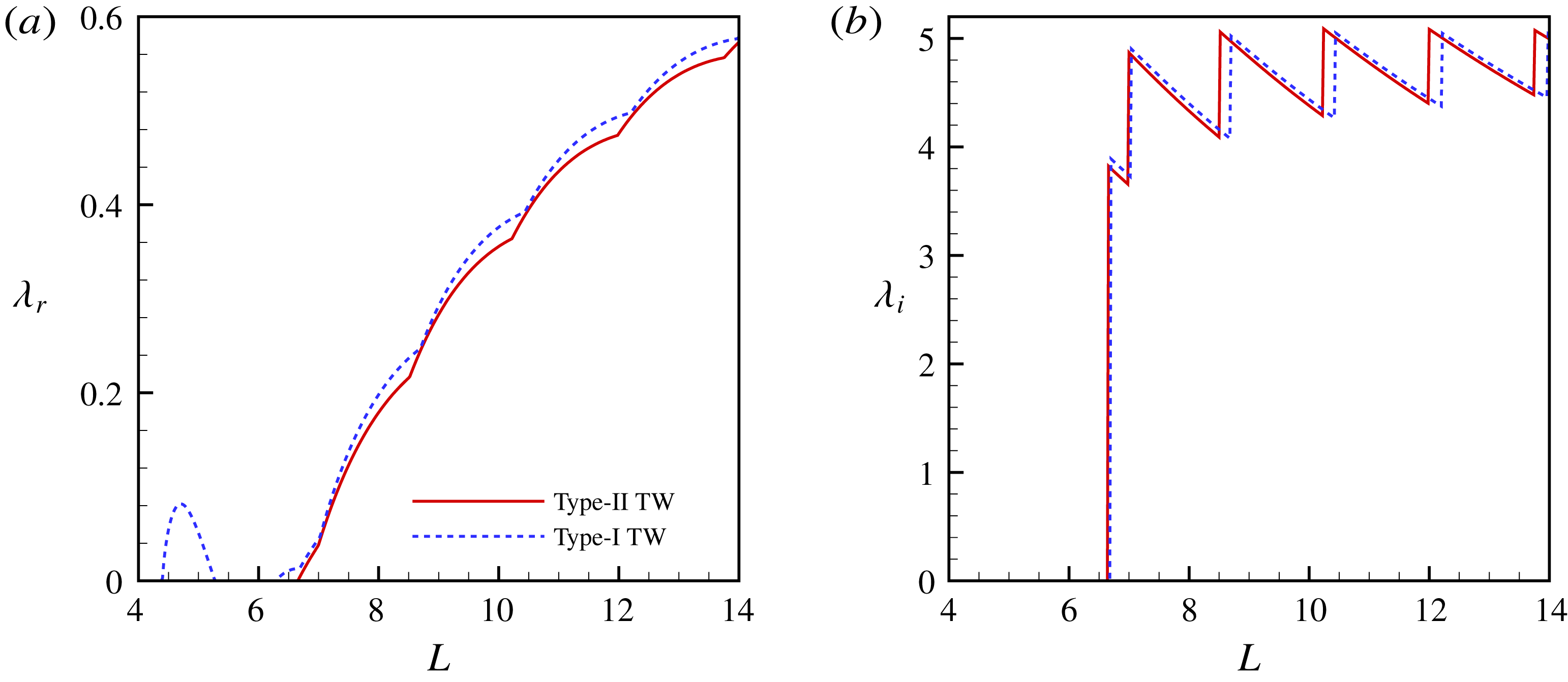
, shown in figure 12. Results in figure 12(a) show that type-II TWs are stable when
 $L\lesssim 6.7$
. Type-I TWs are unstable when
 $4.4\lesssim L\lesssim 5.2$
or
 $L\gtrsim 6.3$
. However, type-I TWs do not lose stability to RPOs when
 $4.4\lesssim L\lesssim 5.2$
, as
 $\unicode[STIX]{x1D706}_{i}=0$
. Figure 12(a,b) demonstrates that the most unstable modes are oscillatory when
 $L\gtrsim 6.7$
for both type-I and type-II TWs, suggesting the existence of RPOs. Interestingly, the sawtooth
 $\unicode[STIX]{x1D706}_{i}{-}L$
curve originates from the mode switching in the system: the growth rate
 $\unicode[STIX]{x1D706}_{r}$
of higher-frequency modes increases faster than that of the low-frequency modes, leading to the switching. Therefore, the frequency of the most unstable mode jumps as
 $L$
increases, leading to the sawtooth structure of the
 $\unicode[STIX]{x1D706}_{i}{-}L$
curve.
(a,b) The leading eigenvalue versus the domain size for type-I and type-II TWs. The dependent parameters are
 $Bo=\unicode[STIX]{x1D716}=0.2$
and
 $\unicode[STIX]{x1D6FC}=0.25$
.

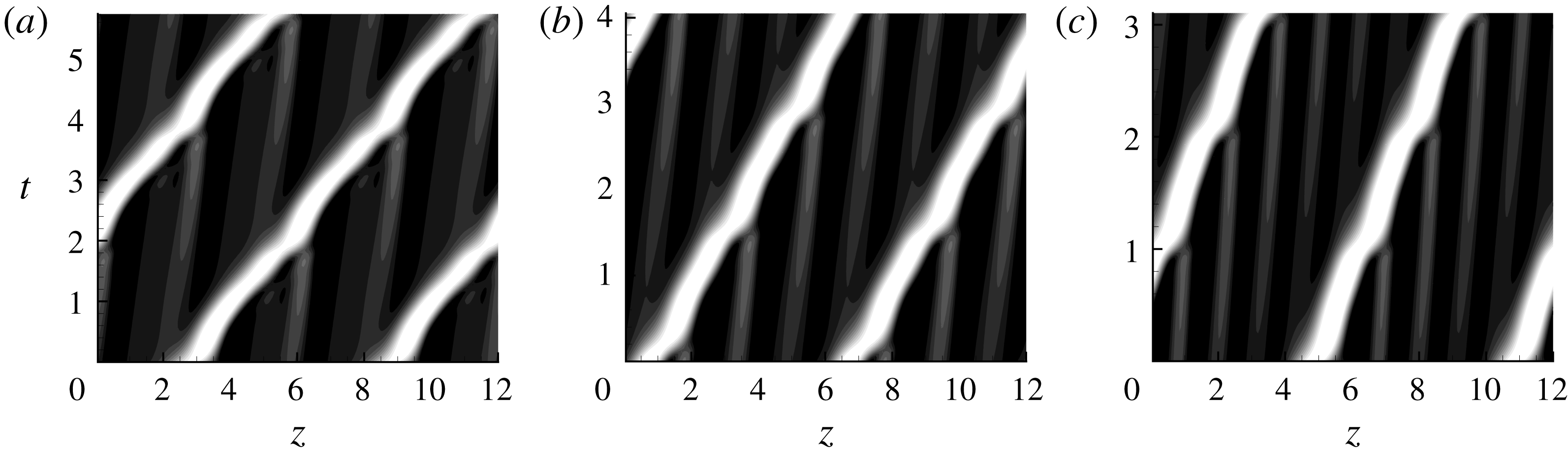
The space–time diagrams for the RPOs plotted in three periods at
 $L=12$
: (a) RPO1 with period
 $T=1.9122$
; (b) RPO2 with period
 $T=1.3501$
; and (c) RPO3 with period
 $T=1.0344$
. The dependent parameters are
 $Bo=\unicode[STIX]{x1D716}=0.2$
and
 $\unicode[STIX]{x1D6FC}=0.25$
.

Numerical simulations were performed in order to obtain initial guesses for the RPOs. We fixed
 $L=12$
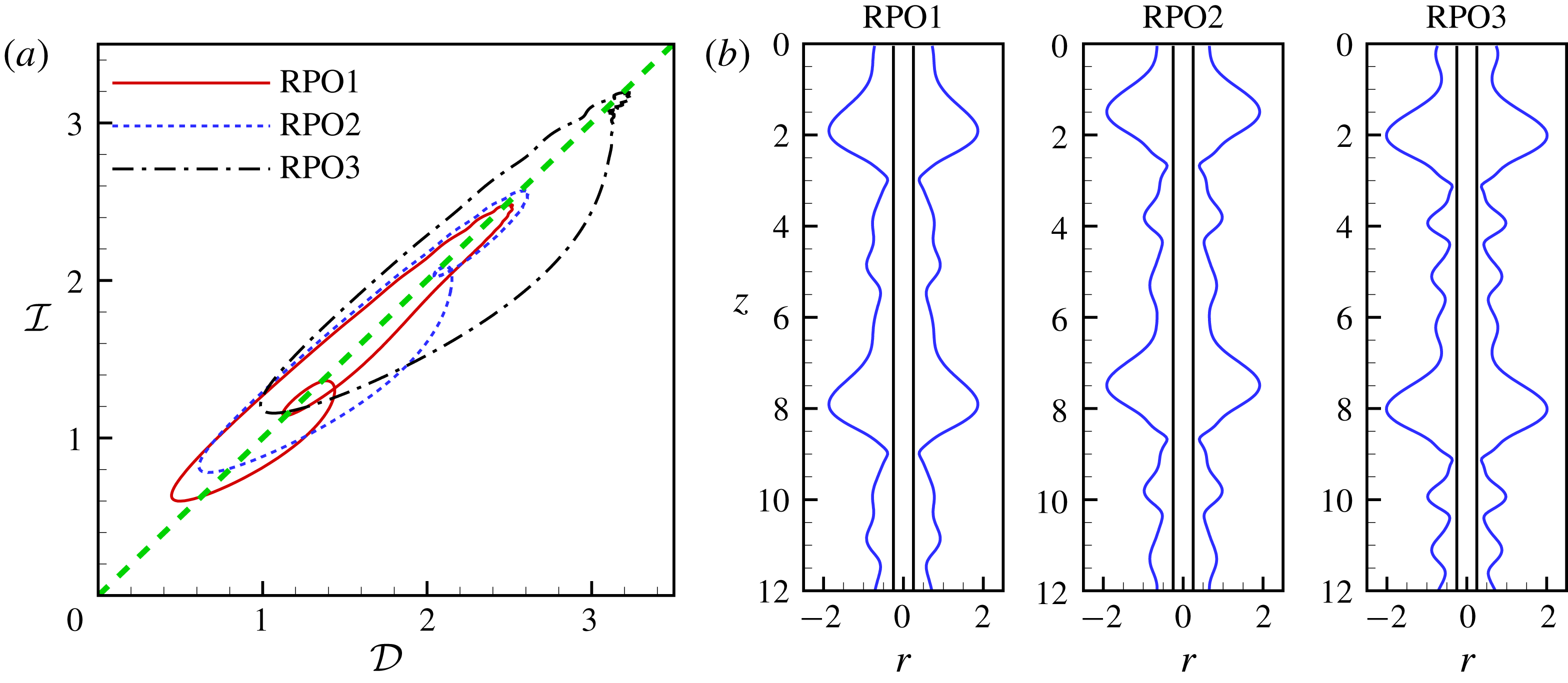
and obtained three converged exact RPOs, namely RPO1, RPO2 and RPO3, whose space–time diagrams are shown in figure 13. We expect that it is possible to find more RPOs of longer period, but we have not pursued this in the present study. The profiles of the three RPOs at some instants in time are shown in figure 14(b). For RPO1, between the two main big droplets, the film is unstable and develops into a ripple-like structure. For RPO2, the unstable film between the two main droplets evolves into two small droplets. For RPO3, there are three small droplets between the two main droplets. As there are more small droplets between the two main droplets, the mean distance between the big droplet and its nearby small droplet decreases. Therefore, it takes less time for the big droplet to consume the nearby small droplet and the oscillation becomes faster, i.e. the periods decrease from RPO1 to RPO3 (see figure 15
a). We observe that the big droplet eats the front small droplet or ripple and itself is unstable at the rear region, which breaks up into new ripples or small droplets. The breakup of the big droplet at its rear region is due to the Plateau–Rayleigh mechanism. Such a cyclic process (also confirmed in figure 14
a) is self-sustaining, which gives the birth of exact RPOs in the non-electrified film.
(a) Three exact RPOs in the
 ${\mathcal{I}}$
–
 ${\mathcal{D}}$
plane at
 $L=12$
. (b) The instant profiles of the liquid films for the RPOs. The dependent parameters are
 $Bo=\unicode[STIX]{x1D716}=0.2$
and
 $\unicode[STIX]{x1D6FC}=0.25$
. Three movies for these RPOs are shown in the supplementary material. Each movie shows three periods of the RPO.

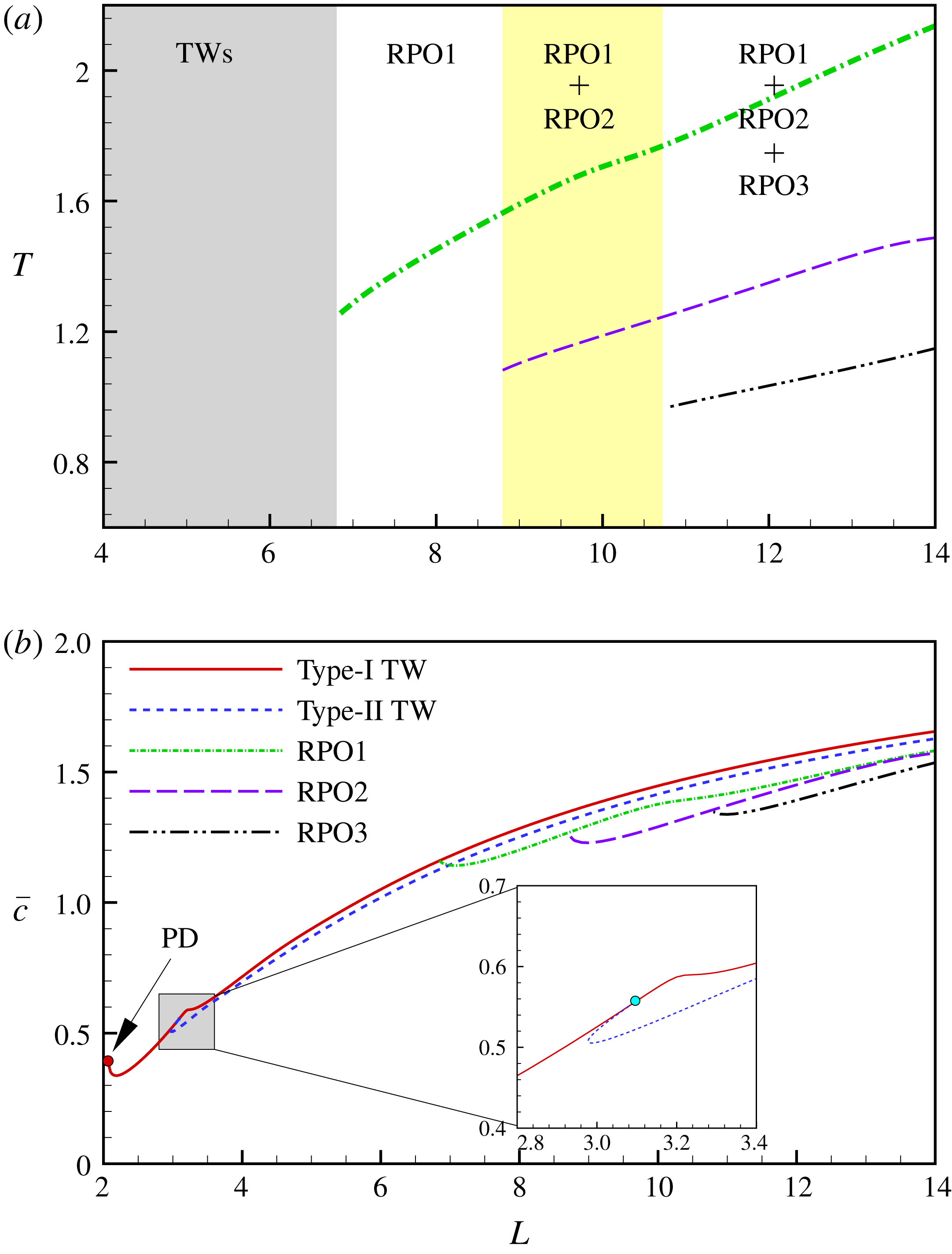
(a) Period
 $T$
versus the domain size
 $L$
for RPOs. Solutions of different regimes are illustrated. When
 $L<6.85$
, only TWs are detected. RPO1 is detected when
 $L>6.85$
; RPO2 is detected when
 $L>8.7$
; and RPO3 is detected when
 $L>10.7$
. (b) The wave speed versus the domain size
 $L$
. The dependent parameters are
 $Bo=\unicode[STIX]{x1D716}=0.2$
and
 $\unicode[STIX]{x1D6FC}=0.25$
. PD stands for period-doubling bifurcation.

It is interesting to investigate how the period and wave speed of the RPO depend on the domain size. Figure 15(a) shows that the period
 $T$
becomes longer as the domain size
 $L$
increases. We speculate that this is because the distance between the big droplet and its front small droplet (the closest one to the big droplet) becomes larger, and therefore longer time is required for the coalescence process. The domain sizes of the three observed different flow regimes in Kliakhandler et al. (Reference Kliakhandler, Davis and Bankhoff2001) are within the current computation, and we do not investigate longer domains in the present study.
Different solution regimes are shown in figure 15(a). RPO1 is not detected when
 $L<6.85$
. The curve for RPO1 in figure 15(b) connects with the type-I TW solution at
 $L\approx 6.85$
. We have verified that the spatial form for RPO1 is very similar to the type-I TW at
 $L=6.85$
, where the ripple between the two big droplets is very small. This indicates that RPO1 is born from the instability of the type-I TW, and explains why we do not detect RPO1 below
 $L=6.8$
. RPO2 and RPO3 were not detected for
 $L\lesssim 8.7$
and
 $10.7$
, respectively. A possible reason why they do not exist in smaller domains may be due to insufficient space for varying numbers of small beads or ripples. The wave speed
 $\bar{c}$
reduces for a stronger oscillation (RPO1 is faster than RPO2, and RPO2 is faster than RPO3). As the domain size
 $L$
increases, the wave speed of RPOs increases (see figures 15
b and 16
c). This is because the average height of the large droplet increases and therefore a faster wave (Craster & Matar Reference Craster and Matar2006). When the domain size is large, although these RPOs can be tracked using numerical continuation, they lose stability and the system is typically chaotic; hence we expect a host of RPOs to describe the droplet coalescence and breakup processes discussed by Craster & Matar (Reference Craster and Matar2006). A selection of the shortest orbits, however, is expected to be sufficient to capture most of the dynamics (Budanur et al.
Reference Budanur, Short, Farazmand and Willis2017).
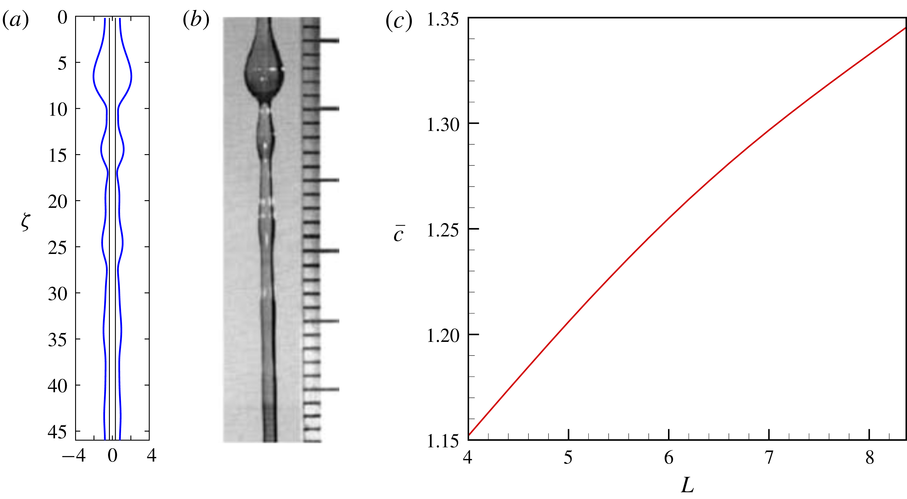
(a) A snapshot of exact RPO. (b) Regime ‘c’ adapted from Kliakhandler et al. (Reference Kliakhandler, Davis and Bankhoff2001). The axis in (a) is rescaled to
 $\unicode[STIX]{x1D701}=z/\unicode[STIX]{x1D716}$
so as to compare with the experimental observation. (c) Wave speed of the RPO versus domain size, in which there is only one big droplet. A movie for the RPO in the supplementary material demonstrates the unsteady flow. The dependent parameters
 $\unicode[STIX]{x1D716}=0.178$
,
 $\unicode[STIX]{x1D6FC}=0.3262$
and
 $L=8.185$
for regime ‘c’ were taken from Craster & Matar (Reference Craster and Matar2006).

Finally, we revisit the experimental study of the flow regime ‘c’ in Kliakhandler et al. (Reference Kliakhandler, Davis and Bankhoff2001), where there is a large droplet with some small ripples at its front. In contrast to the ‘steady’ flow regime ‘b’, the flow regime ‘c’ is an essentially unsteady state due to the droplet coalescence and breakup process (Craster & Matar Reference Craster and Matar2006). Although the TW solution excellently captures the dynamics of flow regime ‘b’, it is questionable whether or not we can compare a ‘steady’ TW with flow regime ‘c’. Craster & Matar (Reference Craster and Matar2006) observed that the large droplet oscillates in the experiment and proposed that flow regime ‘c’ is a superposition of a steady TW and small perturbations. However, their numerical experiment does not compare well with the experimental study, not only in the wave speed but also in the wave profile. In Ruyer-Quil et al. (Reference Ruyer-Quil, Treveleyan, Giorgiutti-Dauphiné and Kalliadasis2008), the streamwise dissipation effect was considered, which leads to a smaller wave speed (
 $c=0.94$
) than in Craster & Matar (Reference Craster and Matar2006). Novbari & Oron (Reference Novbari and Oron2009) used an energy integral model and predicted a bit higher phase speed than Craster & Matar (Reference Craster and Matar2006),
 $c=1.48$
, and the streamwise dissipation effect was neglected by them. (The wave speeds by Ruyer-Quil et al. (Reference Ruyer-Quil, Treveleyan, Giorgiutti-Dauphiné and Kalliadasis2008) and Novbari & Oron (Reference Novbari and Oron2009) are rescaled by
 $W=\unicode[STIX]{x1D70C}h_{0}^{2}g/\unicode[STIX]{x1D707}$
here.) Indeed, Novbari & Oron (Reference Novbari and Oron2009) have realized that flow regime ‘c’ is not a TW because it was unsteady, although they compared it with a TW. All these TWs, however, do not capture a correct film profile: there are no small beads coexisting with the large droplet. Within our set of periodic orbits, we have found profiles of the film very much like experimental observation (figure 16). It should be stressed here that the small droplets/ripples in the front of the big droplet in figure 16 are captured by the RPO, which are not seen in the TW. Kliakhandler et al. (Reference Kliakhandler, Davis and Bankhoff2001) simulated flow regime ‘c’ using their thick film model and showed that these small droplets can survive with big droplets in an unsteady state. The large droplet catches up with and consumes the small droplets in the front, and the rear region of the large droplet breaks up into small droplets. Such a process recurs in the system, i.e. the profile in figure 16(a) appears periodically, which is strikingly similar to that in flow regime ‘c’. Furthermore, the period of the obtained RPO in figure 16(a) is
 $T=1.7156$
. However, no experimental study on RPOs in this film flow was reported, and the period of flow regime ‘c’ in experiments remains unknown. The wave speed of this RPO
 $\bar{c}=1.34$
is a little smaller than the wave speed of the TW,
 $c=1.36$
(Craster & Matar Reference Craster and Matar2006), and is closer to the experimental observation
 $c=0.93$
. Hence, the RPO captures the dynamical scenario, i.e. oscillation, the wave speed of flow regime ‘c’, and the film profile better than the steady TWs, which provides a better understanding of this unsteady state than the TW solution. The mean wave speed predicted by the RPO, however, is still approximately 30 % higher than the measured one. Note that the wave speed of flow regime ‘a’ is correctly predicted by Craster & Matar (Reference Craster and Matar2006). It can be inferred that the 30 % difference is not caused by dropping the inertia term because the Reynolds number in flow regime ‘c’ is much smaller than in flow regime ‘a’. As is shown by Ruyer-Quil et al. (Reference Ruyer-Quil, Treveleyan, Giorgiutti-Dauphiné and Kalliadasis2008), the streamwise viscous dissipation effect can significantly improve the prediction of the wave speed of steady TWs. This suggests that the streamwise diffusion is important when the Reynolds number is small, which is the reason why the predicted wave speed by the asymptotic model is higher than the experimental value.
5 Conclusions
We have investigated a perfectly conducting liquid film flowing down a vertical fibre subject to a radial electric field. The dynamics of the liquid film was examined using a long-wave model. The dynamical systems approach was employed to extract recurrent solutions, i.e. travelling waves (TWs) and relative periodic solutions (RPOs). The Newton–Krylov hook-step method was used to find the RPOs presented in this paper. Two cases were discussed: an electrified film and a non-electrified film.
For the case with an electric field, we investigated the interactions between two big droplets. Numerical simulation showed that the system can evolve into a steady TW state when the electric field is weak. Steady TW solutions, in the form of either two identical droplets (type-I TW) or two slightly different droplets (type-II TW), were tracked. Linear stability analysis shows that the TW solutions become unstable as the electric field exceeds some threshold, and oscillatory instabilities of the TWs develop into RPO solutions. In the oscillatory state, the two droplets are slightly different in size, while two identical droplets do not cause an oscillation unless they are unstable. Interestingly, RPOs were also found through the instability of steady TW solutions in an electrified liquid film flowing down an inclined plane very recently (Lin et al. Reference Lin, Tseluiko, Blyth and Kalliadasis2018).
We have also demonstrated that an electric field has dual effects on the oscillation: the oscillation can be accelerated or decelerated by the electric field. When the electric field is strong, the two droplets merge together, leading to spike-like singular structure.
When the electric field is turned off, several RPOs were found in the non-electrified film. Indeed, steady TWs are also unstable when the domain size exceeds a critical value. RPOs are then found after the instability of the steady TWs. Interestingly, the RPO represents the self-sustaining droplet coalescence and breakup process. The periods and wave speeds of RPOs increase as the domain size increases. An interesting observation is that the wave speed of an RPO is lower than that of the type-I TW, and the motion of droplets is slowed down by the oscillation, no matter if the electric field is imposed or removed.
In addition, the RPO not only captures well the dynamical scenario, but also captures the temporal variation of the wave speed. We find a snapshot of the RPO solution remarkably similar to experimental observation. Together, our results indicate that the RPO provides a better model of the unsteady flow regime in the film flow than the steady TW solution.
Acknowledgements
Z.D. and A.P.W. acknowledge support from an EPSRC grant ‘Optimization in Fluid Mechanics EP/P000959/1’. Z.D. also acknowledges Professor R. R. Kerswell and Dr J. Page for their kind help on the Newton–Krylov hook-step method in Chandler & Kerswell (Reference Chandler and Kerswell2013), which is crucial for the computation of the relative periodic orbits in this study. Z.D. and A.P.W. are also grateful to the three anonymous referees for their many insightful comments, which helped improve the paper significantly.
Supplementary movies
Supplementary movies are available at https://doi.org/10.1017/jfm.2019.450.