Generalizable super-resolution turbulence reconstruction from minimal training data

Haokai Wu; Yong Cao; Yaoran Chen; Shujin Laima; Wen-Li Chen; Dai Zhou; Hui Li

doi:10.1017/jfm.2025.10913

Generalizable super-resolution turbulence reconstruction from minimal training data

Published online by Cambridge University Press: 02 December 2025

Dai Zhou and

Haokai Wu: Affiliation:
School of Ocean and Civil Engineering, Shanghai Jiao Tong University, Shanghai, PR China
Yong Cao*: Affiliation:
School of Ocean and Civil Engineering, Shanghai Jiao Tong University, Shanghai, PR ChinaState Key Laboratory of Ocean Engineering, Shanghai Jiao Tong University, Shanghai, PR China
Yaoran Chen: Affiliation:
School of Future Technology, Shanghai University, Shanghai 200444, PR China
Shujin Laima: Affiliation:
School of Civil Engineering, Harbin Institute of Technology, Harbin, PR China
Wen-Li Chen: Affiliation:
School of Civil Engineering, Harbin Institute of Technology, Harbin, PR China
Dai Zhou: Affiliation:
School of Ocean and Civil Engineering, Shanghai Jiao Tong University, Shanghai, PR ChinaState Key Laboratory of Ocean Engineering, Shanghai Jiao Tong University, Shanghai, PR China
Hui Li: Affiliation:
School of Civil Engineering, Harbin Institute of Technology, Harbin, PR China
*: Corresponding author: Yong Cao, yongcao@sjtu.edu.cn

Article contents

Abstract
Introduction
Methodology
Results and discussions
Conclusions
Funding
Declaration of interests
Code availability
Footnotes
References

Rights & Permissions

Abstract

Fully resolving turbulent flows remains challenging due to a turbulent systems’ multiscale complexity. Existing data-driven approaches typically demand expensive retraining for each flow scenario and struggle to generalize beyond their training conditions. Leveraging the universality of small-scale turbulent motions (Kolmogorov’s K41 theory), we propose a scale-oriented zonal generative adversarial network (SoZoGAN) framework for high-fidelity, zero-shot turbulence generation across diverse domains. Unlike conventional methods, SoZoGAN is trained exclusively on a single dataset of moderate-Reynolds-number homogeneous isotropic turbulence (HIT). The framework employs a zonal decomposition strategy, partitioning turbulent snapshots into subdomains based on scale-sensitive physical quantities. Within each subdomain, turbulence is synthesized using scale-indexed models pretrained solely on the HIT database. A SoZoGAN demonstrates high accuracy, cross-domain generalizability and robustness in zero-shot super-resolution of unsteady flows, as validated on untrained HIT, turbulent boundary layer and channel flow. Its strong generalization, demonstrated for homogeneous and inhomogeneous turbulence cases, suggests potential applicability to a wider range of industrial and natural turbulent flows. The scale-oriented zonal framework is architecture-agnostic, readily extending beyond generative adversarial networks to other deep learning models.

JFM classification

Turbulent Flows: Turbulent boundary layers Turbulent Flows: Homogeneous turbulence Boundary Layers: Boundary layer structure

Information

Type: JFM Papers
Information: Journal of Fluid Mechanics , Volume 1024 , 10 December 2025, A27
DOI: https://doi.org/10.1017/jfm.2025.10913 [Opens in a new window]
Copyright: © The Author(s), 2025. Published by Cambridge University Press

1. Introduction

Turbulence plays a fundamental role across numerous industrial and natural systems, from aerospace engineering to atmospheric dynamics and oceanographic flows. While homogeneous turbulence features spatially uniform statistics, non-homogeneous turbulence – such as wall-bounded flows – exhibits statistical variations driven by boundaries or mean flow gradients. Despite these differences, a central tenet of turbulence theory, Kolmogorov’s K41 hypothesis (Kolmogorov Reference Kolmogorov1941) and its subsequent extensions (Benzi et al. Reference Benzi, Ciliberto, Tripiccione, Baudet, Massaioli and Succi1993), asserts the universality of small-scale turbulent motions at sufficiently high Reynolds numbers. Specifically, statistical properties in the inertial and dissipation ranges become universal: independent of large-scale flow structures and controlled solely by the mean energy dissipation rate $\epsilon$ and the kinematic viscosity $\nu$ . Later studies have further demonstrated that this universality extends beyond velocity statistics to velocity gradient fields. For even-order moments (particularly second-order) of velocity gradients, robust universality is observed across homogenous and non-homogeneous turbulence (Buaria & Pumir Reference Buaria and Pumir2025). Notably, extreme events associated with velocity gradients maintain universal characteristics among various flow configurations, providing a bridge between homogenous and non-homogeneous turbulent regimes (Schumacher et al. Reference Schumacher, Scheel, Krasnov, Donzis, Yakhot and Sreenivasan2014; Buaria et al. Reference Buaria, Clay, Sreenivasan and Yeung2021; Buaria & Pumir Reference Buaria and Pumir2025).

Despite profound theoretical insights, fully resolving turbulent flows remains a formidable challenge. Experimental methods face fundamental spatiotemporal resolution limits (Dunbar et al. Reference Dunbar, van der A, Scandura and O’Donoghue2023), while numerical simulations demand rapidly escalating computational resources with increasing Reynolds number. Direct numerical simulation (DNS) of homogeneous isotropic turbulence (HIT) requires grid counts scaling as $N \sim {\textit{Re}}_{\lambda }^{9/4}$ (Pope Reference Pope2000), with even steeper scaling in wall-bounded flows. Large-eddy simulation (LES) of wall-bounded turbulence imposes significant burdens with $N \sim {Re}^{13/7}$ (Choi & Moin Reference Choi and Moin2012). Such scaling renders high-fidelity simulations infeasible for many practical, high-Reynolds-number flows (Cao et al. Reference Cao, Tamura, Zhou, Bao and Han2022; Yao, Chen & Hussain Reference Yao, Chen and Hussain2022).

Recent advances in deep learning have introduced promising data-driven approaches to these challenges by inferring high-resolution (HR) turbulence features from sparsely sampled or low-resolution (LR) data. These methods learn nonlinear mappings between coarse flow variables and multiscale structures using large datasets, achieving notable success in reconstructing detailed turbulent fields (Manohar et al. Reference Manohar, Brunton, Kutz and Brunton2018; Fukami, Fukagata & Taira Reference Fukami, Fukagata and Taira2019; Brunton, Noack & Koumoutsakos Reference Brunton, Noack and Koumoutsakos2020; Fukami et al. Reference Fukami, Maulik, Ramachandra, Fukagata and Taira2021b ; Vinuesa & Brunton Reference Vinuesa and Brunton2022; Lozano-Durán & Bae Reference Lozano-Durán and Bae2023; Cuéllar et al. Reference Cuéllar, Güemes, Ianiro, Flores, Vinuesa and Discetti2024). Among these, super-resolution (SR) frameworks – originally developed for image processing – aim to produce HR flow fields $\boldsymbol{q}_{\textit{HR}} \in \mathbb{R}^{n_x \times n_y}$ from coarse inputs $\boldsymbol{q}_{\textit{LR}} \in \mathbb{R}^{(n_x/r) \times (n_y/r)}$ , where $r$ is the downsampling factor. These models infer unresolved turbulent motions from coarse data, bridging the gap between limited-resolution simulations or experiments and the full turbulence spectrum.

Deterministic neural networks, such as convolutional neural networks (CNNs) (Guan et al. Reference Guan, Chattopadhyay, Subel and Hassanzadeh2022; Fukami et al. Reference Fukami, Fukagata and Taira2023, Reference Fukami, Goto and Taira2024) and graph neural networks (Han et al. Reference Han, Gao, Pfaff, Wang and Liu2022), have been pioneering tools in turbulence SR due to their ability to extract local and non-Euclidean features, respectively. However, their deterministic nature limits their capacity to capture the inherently stochastic, high-dimensional dynamics of turbulence, especially in regimes dominated by chaotic small-scale fluctuations (Du et al. Reference Du, Parikh, Fan, Liu and Wang2024).

More recently, generative models have brought a paradigm shift by integrating probabilistic learning into turbulence SR. Super-resolution generative adversarial networks (SRGANs) (Stengel et al. Reference Stengel, Glaws, Hettinger and King2020; Yasuda & Onishi Reference Yasuda and Onishi2023; Cuéllar et al. Reference Cuéllar, Güemes, Ianiro, Flores, Vinuesa and Discetti2024; Page Reference Page2025) – including Wasserstein generative adversarial networks (GANs) (Gao & Ng Reference Gao and Ng2022), conditional GANs (Mirza & Osindero Reference Mirza and Osindero2014) and CycleGAN (Kim et al. Reference Kim, Kim, Won and Lee2021) – as well as diffusion-based models (Dhariwal & Nichol Reference Dhariwal and Nichol2021; Gao et al. Reference Gao, Liu, Zeng, Xu, Li, Luo, Liu, Zhen and Zhang2023), reconstruct microscale turbulence in a statistically consistent manner through adversarial or hierarchical training. Extensions of this line of research include the integration of SR into subgrid-scale modelling for very coarse LES data, thereby linking deep learning-based reconstruction with turbulence modelling theory through conditional GAN (supervised) and CycleGAN (unsupervised) frameworks (Maejima & Kawai Reference Maejima and Kawai2025). Notably, SRGANs preserve turbulent energy spectra and dissipation mechanisms, enhancing physical fidelity (Stengel et al. Reference Stengel, Glaws, Hettinger and King2020; Kim, Kim & Lee Reference Kim, Kim and Lee2024; Wu et al. Reference Wu, Zhang, Zhou, Chen, Han and Cao2024). Hybrid frameworks combining normalizing flows and graph neural networks further enable probabilistic generation of instantaneous turbulent fields (Sun et al. Reference Sun, Han, Gao, Wang and Liu2023). Although such methods reconcile deterministic approximations with turbulent stochasticity, their training remains computationally expensive, particularly when resolving multiscale interactions.

Two major limitations persist in current data-driven turbulence SR methods. First, existing models exhibit limited generalization ability beyond their training datasets; adapting to new turbulence conditions often requires costly retraining or fine-tuning with high-fidelity data (Santos et al. Reference Santos, Fox, Mohan, O’Malley, Viswanathan and Lubbers2023; Fukami & Taira Reference Fukami and Taira2024; Li et al. Reference Li, Han, Zhang, Fu, Li, Qin, Dong, Sun, Deng and Yang2024). Second, achieving broad generalizability typically demands extensive, HR, multicondition datasets (Güemes et al. Reference Güemes, Sanmiguel Vila and Discetti2022), whose generation imposes substantial computational burdens and hinders scalability. These challenges arise primarily due to the vast variability of flow patterns and boundary effects encountered in practical applications, which are often not well represented in training data. Recent efforts have tackled the training-data scarcity problem by leveraging efficient sampling strategies. Notably, Fukami & Taira (Reference Fukami and Taira2024) proposed a multiscale extraction approach, in which subdomains of various vortical sizes are cropped from a single instantaneous HR flow field to construct a diverse set of training samples across scales. This method exploits the spatial scale similarity inherent in turbulence to synthetically enrich the training dataset, thereby substantially alleviating the need for multiple training datasets.

To address two longstanding challenges in turbulence SR – limited generalization and high data dependence – this work leverages the universality concept of small-scale turbulent motions to propose the scale-oriented zonal GAN (SoZoGAN). This innovative framework enables efficient, high-fidelity SR by generalizing across diverse flow regimes using only coarse input fields. The SoZoGAN operates in a ‘zero-shot’ manner: it predicts small-scale turbulent structures in unseen flow configurations without retraining or labelled data from the new target tasks (Xian et al. Reference Xian, Lampert, Schiele and Akata2019). Unlike conventional approaches, SoZoGAN is pretrained exclusively on a single, readily accessible dataset: HIT at moderate Reynolds number. Leveraging a carefully designed scaling transformation of HIT data, we construct a library of scale-specific SRGAN models that span a wide range of turbulent scales, conceptually akin to the multiscale extraction approach of Fukami & Taira (Reference Fukami and Taira2024). To adapt to spatially inhomogeneous flows, the framework partitions target fields into subdomains based on scale-sensitive physical quantities. Each subdomain is then super-resolved using the pretrained SRGAN model corresponding to its characteristic scale. By synergistically coupling offline scale-specific pretraining with online zero-shot synthesis, SoZoGAN delivers robust cross-domain performance. Furthermore, the scale-oriented zonal strategy is model-agnostic and can be integrated flexibly with diverse deep learning architectures beyond GANs.

2. Methodology

2.1. Overview

Turbulent flows in practical scenarios often exhibit pronounced anisotropy and inhomogeneity due to disturbances originating either within the flow or near boundaries. These effects cause the characteristic turbulent scales to vary significantly across different spatial regions of the global flow field. Such spatial scale variability poses a major challenge for turbulence SR, because a single SR model – trained under fixed-scale assumptions – cannot simultaneously recover flow structures across all local regions with high physical fidelity. Consequently, an adaptive SR framework is needed to (i) identify locally varying physical scales, and (ii) apply scale-appropriate generative models without retraining for each new case.

Figure 1.

The SoZoGAN framework for turbulence SR that generalizes across diverse turbulent flows using ‘zero-shot’ transfer. (a) Establishment of a pretrained SR model library using a single dataset. (b) Zonal decomposition and microscale estimation based on the LR flow field. (c) Microscale alignments of the decomposed subdomains and the procedure of ‘zero-shot’ generation from LR subdomains to the SR global flow field. (d) Test cases of the proposed framework, including HIT, turbulent boundary layer (TBL) and channel flow.

To address this challenge, we propose the SoZoGAN, a ‘zero-shot’ SR framework designed for high-fidelity reconstruction of inhomogeneous turbulence without additional training or fine-tuning for new flow scenarios. The central idea is to exploit the universality of small-scale turbulent motions, learned from a single HIT dataset, and transfer this SR capability to diverse target flows through a scale-oriented decomposition and model-alignment workflow. As illustrated in figure 1, SoZoGAN operates in three connected stages, each with a clear motivation as follows.

(i) Microscale-indexed model pretraining (figure 1 a). Starting from HIT data, a carefully designed scaling transformation generates training samples covering a wide range of microscale conditions. For each distinct microscale, a dedicated SRGAN is pretrained, forming a library of scale-specific models indexed by their microscale values. This offline stage is designed to encapsulate scale-dependent generative characteristics into specialized models, thereby eliminating the need for retraining in subsequent target cases (see § 2.2).
(ii) Zonal decomposition and microscale estimation (figure 1 b). The LR target field is partitioned into subdomains with approximately uniform scale features, based on scale-sensitive quantities such as velocity fluctuations, velocity gradients or spectral content. An multilayer perceptron (MLP)-based estimator then predicts the characteristic microscale of each subdomain directly from LR inputs. This stage helps to align each subdomain to the most suitable pretrained SRGAN in a physically grounded way, preventing global heterogeneity from biasing local scale identification (see § 2.3).
(iii) Scale-oriented zero-shot generation (figure 1 c). For each subdomain, the SRGAN whose microscale index best matches the estimated local scale is retrieved from the library. The subdomains are super-resolved individually without retraining, and the resulting SR patches are blended to reconstruct a globally continuous field. This stage aims to deploy specialized priors where they fit best, while ensuring seamless global integration through blending and continuity handling (see § 2.4).

By coupling offline scale-indexed pretraining with online scale-aware deployment, SoZoGAN bridges the gap between single-dataset training and generalized SR across spatially heterogeneous turbulence, enabling zero-shot reconstructions for previously unseen flow configurations.

2.2. Pretrained model library

Homogeneous and isotropic turbulence is the most fundamental and widely applicable type of turbulence. In terms of its generation mechanism, the multiscale similarity observed in isotropic turbulence is also present in other turbulence types, all of which adhere to the energy cascade theory. This provides a theoretical foundation for data-driven models trained on isotropic turbulence data to be ‘zero-shot’ transferred to different turbulence types. Therefore, in the pretraining stage, the public database of DNS HIT (Yeung, Zhai & Sreenivasan Reference Yeung, Zhai and Sreenivasan2015) made available by the Johns Hopkins Turbulence Databases (JHTDB) is employed to exclusively pretrain the SR models.

To generate turbulent flow fields with spatially varying scale characteristics, we require a set of SR models, each pretrained to learn a corresponding structural pattern at a specific characteristic scale (microscale). The pretraining data, which capture distinct turbulence features at these characteristic scales, are manually extended from the single HIT dataset using a physics-related scaling transformation. Each SR model is pretrained on specific data that represent a microscale and is indexed accordingly with the corresponding scale value, as illustrated in figure 1(a).

In the final step, these pretrained SR models are organized into a model library. This library facilitates efficient model retrieval during the following ‘zero-shot’ generation stage, enabling the appropriate model to be selected based on the required scale characteristics. The implementation details of data curation and model pretraining are provided below.

2.2.1. Data curation

The pretraining HIT database was simulated within a $x\times y\times z = 2\pi \times 2\pi \times 2\pi$ box using pseudospectral method, with a grid size of $8192\times 8192\times 8192$ . Five three-dimensional snapshots are collected in this database with $Re_{\lambda }\sim 1200$ . In each snapshot, three velocity components of $u$ , $v$ and $w$ are included for $x$ , $y$ and $z$ directions.

Since this study focuses on two-dimensional spatial SR, pretraining samples of velocity distribution planes are extracted from each snapshot, as illustrated in figure 2(a). To obtain these samples, we first extract 50 equally spaced $x$ – $y$ slices along the $z$ -direction for each snapshot, ensuring uniform coverage of streamwise–spanwise structures throughout the HIT data. Within each extracted $x$ – $y$ slice, we partition along the $y$ -direction into three non-overlapping rectangular planes, each with a size of $x \times y = 2\pi \times 0.5\pi$ (grid resolution $8192 \times 2048$ ). These partitioned planes constitute our initial sample planes. Applying this procedure to all five snapshots yields a total of $50 \times 3 \times 5 = 750$ initial planes for pretraining.

Figure 2.

Data curation from a single HIT dataset and verification of the scaling transformation method: (a) schematic of the spatial and temporal sampling procedure to obtain initial planes, followed by (b) extension into velocity subplanes. Scaling transformation is applied to extract subplane samples with different microscales from the initial planes. The numbers labelled in the top right-hand corner of each subplane ( $\gamma$ ) represent the scaling ratios in the $x$ or $y$ direction relative to the width or height of the initial plane. (c) Validity of the scaling transformation. The scaling ratios $\gamma$ and the Taylor microscales $\lambda ^{\prime}_{\gamma }$ are nearly in a linear relationship for a series of HIT subplanes.

In our pretraining stage, for scale-oriented learning of a set of SR models, HIT samples with varying Taylor microscales are artificially extracted from a single original dataset. Leveraging the self-similarity of turbulence, a scaling method is applied to crop the initial sampled plane ( $2\pi \times 0.5\pi$ ) proportionally in both the $x$ and $y$ directions, creating multiple subplanes in figure 2(b) (grid resolution $8192/\gamma \times 2048/\gamma$ ). The $\gamma$ ( $\gamma \geqslant 1$ ) labelled in the top right-hand corner of each subplane represents the scaling ratio in the $x$ or $y$ direction relative to the width or height of the initial sampled plane. Simultaneously, the space length of each subplane should be rescaled to the initial plane ( $2\pi \times 0.5\pi$ ) to reproduce the larger-scale distribution characteristics from the cropped smaller-scale ones. This operation purposely filters out smaller-scale turbulent structures from the original HIT data, thereby preserving larger-scale turbulence features in the extended subplane samples. Through a series of scaling transformations, pretraining samples with diverse feature scales are obtained.

To assess the validity of this scaling transformation, it is necessary to examine the relationship between the scaled physical properties (specifically, the Taylor microscale) and the scaling ratio $\gamma$ . The Taylor microscales of subplane samples with varying $\gamma$ are calculated as $\lambda_{\gamma}^{\prime2} = 2 \langle u^2 \rangle / \langle [ \partial u / \partial y ]^2 \rangle$ (Pope Reference Pope2000), where the coordinate $y$ is consistent with that of the initial sampled plane. The operator $\left \langle \boldsymbol{\cdot }\right \rangle$ denotes the statistical mean over 750 subplane samples at each corresponding $\gamma$ . As shown in figure 2(b), $\gamma$ and $\lambda _\gamma ^{\prime}$ are generally positively correlated in a linear relationship. It indicates that ${\lambda _\gamma ^{\prime}} \approx \gamma \boldsymbol{\cdot }\lambda _1^{\prime}$ . Therefore, by adjusting $\gamma$ based on $\lambda _1^{\prime}$ ( $\sim 0.0331$ ) of the original HIT field, we can easily obtain the corresponding pretraining samples for the desired Taylor microscale of $\lambda _\gamma ^{\prime}$ .

2.2.2. Pretrained SRGAN models

Unlike conventional supervised regression models that rely solely on specific network architectures, such as MLPs (Rumelhart, Hinton & Williams Reference Rumelhart, Hinton and Williams1986) or CNNs (Lecun et al. Reference Lecun, Bottou, Bengio and Haffner1998), a GAN is a training framework that can be instantiated with different architectures. In image SR tasks, both generator and discriminator components of a GAN are often implemented as CNNs, adversarially trained to enhance the fidelity of fine-scale structures. Such adversarial training is particularly effective at recovering high-frequency content and complex microscale details in the reconstructed fields.

In the SoZoGAN framework, all SR models follow the SRGAN design proposed by Wang et al. (Reference Wang, Wu, Su, Duan and Wang2019), where the generator ( $G$ ) and discriminator ( $D$ ) are jointly trained within an adversarial learning paradigm. Both $G$ and $D$ employ CNN-based architectures. The detailed architectures of $G$ and $D$ follow prior deep-learning-based SR studies (Wang et al. Reference Wang, Wu, Su, Duan and Wang2019; Wu et al. Reference Wu, Chen, Xie, Zhou, Tamura, Zhang, Cao and Cao2023, Reference Wu, Zhang, Zhou, Chen, Han and Cao2024).

Let the HR reference flow field be $\boldsymbol{q}_{\textit{HR}} \in \mathbb{R}^{n_x \times n_y}$ , and the corresponding LR input be $\boldsymbol{q}_{\textit{LR}} \in \mathbb{R}^{(n_x/r) \times (n_y/r)}$ , where $r$ is the downsampling factor. In the supervised pretraining stage, $\boldsymbol{q}_{\textit{LR}}$ is obtained from $\boldsymbol{q}_{\textit{HR}}$ via a downsampling (average pooling) operator $\mathcal{D}$ , i.e. $\boldsymbol{q}_{\textit{LR}} = \mathcal{D}(\boldsymbol{q}_{\textit{HR}})$ . The adversarial training of SRGAN is formulated as

(2.1)

\begin{equation} \min _{G} \max _{D} V(D, G) = \mathbb{E}_{\boldsymbol{q}_{\textit{HR}} \sim p_{{\textit{data}}}}\, \big[\log D(\boldsymbol{q}_{\textit{HR}}) \big] + \mathbb{E}_{\boldsymbol{q}_{\textit{LR}} \sim p_{n}}\, \big[\log (1 - D(G(\boldsymbol{q}_{\textit{LR}})))\big] , \end{equation}

where $p_{{\textit{data}}}$ and $p_{n}$ denote the probability distributions of HR and LR samples, respectively. It is important to note that HR data $\boldsymbol{q}_{\textit{HR}}$ are required only during the pretraining stage, where they serve as supervised targets for learning both $G$ and $D$ . Once the scale-indexed SRGAN library has been trained, the zero-shot prediction stage operates solely on LR inputs $\boldsymbol{q}_{\textit{LR}}$ without any need for HR references. In inference, $G$ produces SR reconstructions $\hat {\boldsymbol{q}}_{\textit{HR}} = G(\boldsymbol{q}_{\textit{LR}})$ , recovering small-scale turbulent structures using the scale-specific representations acquired during pretraining.

During pretraining, the generator $G$ in each SRGAN is optimized with paired LR and HR fields. The training objective integrates pixelwise accuracy, adversarial error and physical consistency via a composite loss,

(2.2)

\begin{equation} L_G = L_{{\textit{MSE}}} + \alpha \, L_{\textit{Ad}v\textit{er}} + \beta \, L_{{\textit{Conti}}}, \end{equation}

where

(2.3)

\begin{equation} L_{{\textit{MSE}}} = \| \boldsymbol{q}_{\textit{HR}} - G(\boldsymbol{q}_{\textit{LR}}) \|_2^2, \end{equation}

penalizing the $\ell _2$ error between the SR reconstruction and its HR reference,

(2.4)

\begin{equation} L_{\textit{Ad}v\textit{er}} = - \log \big (D(G(\boldsymbol{q}_{\textit{LR}}))\big ), \end{equation}

where $D(\boldsymbol{\cdot })$ estimates the probability that a sample belongs to the HR distribution (Stengel et al. Reference Stengel, Glaws, Hettinger and King2020), encouraging $G$ to produce perceptually realistic outputs, and

(2.5)

\begin{equation} L_{{\textit{Conti}}} = \left \| \frac {\partial u}{\partial x} + \frac {\partial v}{\partial y} + \frac {\partial w}{\partial z} \right \|_{2,{SR}}, \end{equation}

where $L_{{\textit{Conti}}}$ denotes the $\ell _2$ norm of the divergence of the reconstructed SR velocity field $(u, v, w)$ , computed using finite-difference approximations. This term enforces the incompressible continuity constraint during training. To calculate $\partial w/\partial z$ in $L_{{\textit{Conti}}}$ , the SRGAN should also generate the SR $w$ -component on the neighbouring $x$ – $y$ plane, following the strategy employed by Wu et al. (Reference Wu, Zhang, Zhou, Chen, Han and Cao2024).

The balancing factors $\alpha$ and $\beta$ control the influence of the adversarial and physics-based terms; $\alpha$ is fixed to $10^{-3}$ following Stengel et al. (Reference Stengel, Glaws, Hettinger and King2020), while $\beta$ is adapted so that $L_{{\textit{Conti}}}$ constitutes more than 50 % of $L_G$ on average, ensuring a strong emphasis on physical consistency. As noted above, HR data $\boldsymbol{q}_{\textit{HR}}$ are used solely for pretraining; in the subsequent zero-shot prediction stage, $G$ operates exclusively on LR inputs $\boldsymbol{q}_{\textit{LR}}$ without requiring HR references.

To construct HR–LR training pairs, we treat all pretraining samples derived from the HIT dataset as HR velocity fields. Each HR field has dimensions $8192/\gamma \times 2048/\gamma \times 3$ (corresponding to the three velocity components) and is associated with a specific Taylor microscale $\lambda _\gamma ^{\prime}$ . The corresponding LR inputs are generated by applying average pooling with downsampling factor $r$ , where $r$ also corresponds to the desired SR ratio. This produces LR fields of dimensions $8192/(\gamma \boldsymbol{\cdot }r) \times 2048/(\gamma \boldsymbol{\cdot }r) \times 3$ . We therefore build a library of pretrained $r\times$ SRGAN models, with each model uniquely indexed by its Taylor microscale $\lambda _\gamma ^{\prime}$ .

Average pooling here is both computationally efficient and physically interpretable as an explicit low-pass filtering process. In our study, the generated LR data are obtained through a well-controlled pooling that preserves large-scale, energy-containing structures and part of the inertial-range dynamics, while filtering out unresolved motions. This makes it suitable for obtaining LR data not only from numerical simulations but also from experimental measurements such as particle image velocimetry or multifidelity regridded datasets (Scarano Reference Scarano2013; Fukami et al. Reference Fukami, Fukagata and Taira2019, Reference Fukami, Maulik, Ramachandra, Fukagata and Taira2021b ). Compared with our previous work (Wu et al. Reference Wu, Zhang, Zhou, Chen, Han and Cao2024), which applied an additional low-pass filter after pooling to mimic small-scale energy dissipation in very coarse-grid simulations, the present study omits this step to solely considerate the resolution-scale effects. Nonetheless, the SRGAN-based energy-cascade model (EC-SRGAN) model proposed by Wu et al. (Reference Wu, Zhang, Zhou, Chen, Han and Cao2024) can be integrated into the current framework to form a ‘SoZoEC–SRGAN’ variant for targeted small-scale reconstruction in very coarse-grid simulation scenarios. Extended work will specifically address these extreme scenarios in § 3.7.

2.3. Physics-guided zonal decomposition and microscale estimation

The generation of small scales in inhomogeneous turbulence poses a fundamental challenge: how can we recover local small-scale structures when the input field exhibits dramatic spatial variations in its characteristic scales? Traditional SR approaches, which treat the entire domain uniformly, inevitably fail when confronted with such heterogeneity. To address this limitation, we propose decomposing the LR input field into physically informed subdomains, where characteristic microscales are estimated or precalibrated within each subdomain to guide subsequent turbulence generation.

2.3.1. Zonal decomposition through hierarchical clustering

We first illustrate the zonal decomposition process using wall-bounded turbulence, a canonical example of strongly inhomogeneous flow. Such flows are typically homogeneous in the horizontal directions but exhibit pronounced variations in turbulence statistics along the wall-normal direction. This anisotropy calls for a decomposition strategy that explicitly respects spatial differences in turbulent scales.

In the SoZoGAN, zonal decomposition is not an independent preprocessing step but a prerequisite for physics-based microscale estimation. Partitioning the domain into subdomains with relatively uniform scale properties ensures that the estimated microscale parameters are representative of each subdomain, rather than being distorted by mixed-scale statistics. Without this step, parameter estimation would be less accurate, undermining the effectiveness of scale-specific SR model selection. To achieve this, we employ a hierarchical clustering approach based on scale-sensitive physical quantities extracted from the LR input field (figure 1 b, ‘zonal decomposition’ panel). This method produces subdomains within which turbulence scales remain consistent, enabling physically meaningful subdomains for targeted SR reconstruction. The procedure for wall-bounded turbulence proceeds in four systematic steps.

First, we divide the coarse flow field into local grid groups, each containing points at the same wall-normal height, where turbulence statistics are approximately comparable. These groups form the fundamental units for hierarchical clustering.

Second, for each group, we compute scale-sensitive physical quantities from the coarse input field. Specifically, the one-dimensional wavenumber spectra of all three velocity components are calculated along the statistically homogeneous horizontal direction. These spectra describe the distribution of turbulent kinetic energy (TKE) across spatial scales at each wall-normal location and serve as feature vectors for clustering.

While one-dimensional wavenumber spectra are used in this study for their clear physical interpretation and ability to represent the full turbulence scale distribution, the proposed zonal decomposition is not limited to this choice. Other scale-sensitive quantities – such as velocity gradient magnitude, TKE or eddy size from autocorrelation lengths – can also serve as clustering features, and multiple quantities may be combined if appropriately normalized. For the wall-bounded turbulence considered here, the one-dimensional spectra are chosen because they (i) link directly to turbulence scales, revealing both dominant and dissipative ranges, (ii) exploit directional homogeneity to reduce noise and isolate genuine wall-normal scale variations and (iii) offer richer multiscale detail than single-point measures, enabling more discriminative subdomain clustering.

Third, similarity between groups is measured as the Euclidean distance between their spectral feature vectors, giving $m(m-1)/2$ pairwise distances for $m$ groups. Hierarchical clustering with an average linkage criterion is then applied, iteratively merging wall-normal locations with the highest spectral similarity. The average distance between two merged clusters $C_1$ and $C_2$ is defined as

(2.6)

\begin{equation} d(C_{1}, C_{2})=\frac {1}{|C_{1}||C_{2}|} \sum _{x_{1} \in C_{1}} \sum _{x_{2} \in C_{2}} d(x_{1}, x_{2}), \end{equation}

where $|C_{1}|$ and $|C_{2}|$ are the numbers of groups in each cluster, and $d(x_{1}, x_{2})$ is the Euclidean distance of the spectral feature vectors between local grid groups $x_{1}$ and $x_{2}$ . This criterion promotes the formation of clusters with coherent scale characteristics.

While Euclidean distance is adopted here for its computational simplicity, numerical stability and compatibility with the average-linkage criterion, the zonal decomposition can readily incorporate other similarity measures. For example, if spectral features are normalized as probability distributions, distribution-based metrics such as the Kullback–Leibler divergence or the Wasserstein-2 distance (Lienen et al. Reference Lienen, Lüdke, Hansen-Palmus and Günnemann2024) can be used to capture differences in the shape of the energy spectrum.

Finally, the hierarchical clustering process produces a dendrogram (‘tree-shaped structure’) in which each local grid group starts as an individual leaf node and, at each iteration, the pair with the smallest average intercluster distance is merged into a new parent node (Zhao, Karypis & Fayyad Reference Zhao, Karypis and Fayyad2005; Patel, Sihmar & Jatain Reference Patel, Sihmar and Jatain2015). This process continues until a single root is reached, with the vertical axis of the dendrogram representing the distance at which merges occur. The final decomposed subdomains are obtained by ‘cutting’ this tree horizontally at a specified maximum intercluster distance: a smaller threshold preserves finer wall-normal scale variations by producing more subdomains, whereas a larger threshold yields fewer, coarser partitions. By tuning this distance, one can balance computational efficiency against the need to capture spatial variations in turbulence scales. The resulting adaptive decomposition maintains horizontal homogeneity within each layer while retaining the wall-normal variation of scales, ensuring that each subdomain is well suited for targeted SR.

Although the above steps are presented for wall-bounded turbulence, the hierarchical clustering is generally applicable to other non-homogeneous turbulence types by adapting the definition of the fundamental units. For example, in atmospheric turbulence, where significant inhomogeneity exists in both longitudinal and latitudinal directions, the fundamental unit can be defined as a rectangular region in the plane (figure 1 b). The size of this rectangle determines the granularity of the zonal decomposition – smaller rectangles can better capture local turbulence variability. This flexibility makes the approach broadly adaptable to diverse flow configurations.

2.3.2. Physical basis for microscale estimation

The Taylor microscale $\lambda$ has a unique position in turbulence theory, marking the crossover between the energy-containing and dissipation ranges of the turbulent cascade (Pope Reference Pope2000). It characterizes the length scale over which small-scale velocity fluctuations remain correlated, making it a central anchor for SR reconstruction. However, coarse-grained fields typically capture only the large-scale motions, leaving microscale information severely underrepresented or entirely absent.

The key insight is to exploit the intrinsic relationships that govern turbulent scales. According to Kolmogorov’s similarity theory, the Taylor microscale is fundamentally linked to large-scale energetics through the energy cascade mechanism. For isotropic turbulence, this relationship takes the form (Pope Reference Pope2000)

(2.7)

\begin{equation} \lambda / L=\sqrt {10} {\textit{Re}}_{L}^{-1/2},\quad {\textit{Re}}_{L}\equiv k_t^{1/2} L/\nu, \end{equation}

where ${\textit{Re}}_{L}$ is the large-scale Reynolds number, $L$ is the integral length scale characterizing the energy-containing eddies, $k_t=( {3}/{2})\overline {u^{\prime 2}}$ is the TKE, $u^{\prime}$ is the root-mean-square velocity fluctuation and $\nu$ is the kinematic viscosity.

Equation (2.7) reveals a profound physical truth: even when microscale structures are not visible in coarse data, their characteristic scales remain encoded in the macroscale flow properties. This relationship suggests that a mapping function $\mathcal{F}: \lambda = f(L, u^{\prime}, \nu )$ may exist for more general turbulent flows. To approximate this mapping for complex inhomogeneous turbulence, we employ a MLP architecture, as illustrated in figure 1(b). This neural network serves as a physical anchor, translating available macroscale information from coarse inputs into estimates of the embedded microscales. The following § 2.3.3 provides details on its input–output mapping, training datasets, loss formulation and optimization strategy.

2.3.3. Microscale estimation via pretrained MLP

Once the flow field is decomposed into physically coherent subdomains, each subdomain requires microscale calibration to guide the selection of appropriate SR models. Our MLP architecture, featuring three hidden layers with eight neurons each, undertakes this mapping from macroscale flow parameters to embedded Taylor microscales ( $\mathcal{F}: \lambda = f(L, u^{\prime}, \nu )$ ), as depicted in figure 1(b).

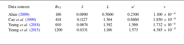
The MLP is trained using a diverse collection of HIT databases (Cao, Chen & Doolen Reference Cao, Chen and Doolen1999; Aluie Reference Aluie2009; Yeung et al. Reference Yeung, Zhai and Sreenivasan2015, Reference Yeung, Sreenivasan and Pope2018), as detailed in table 1. These datasets span a broad range of flow conditions, enabling the network to learn varied scale relationships. The macroscale quantities – integral length scale $L$ , root-mean-square velocity fluctuation $u^{\prime}$ and kinematic viscosity $\nu$ – are extracted from LR fields and serve as the network input. These three quantities together determine the large-scale Reynolds number $Re_{L}$ , which, under isotropic turbulence scaling, relates to the Taylor Reynolds number as $Re_{\lambda }\propto Re_{L}^{1/2}$ . Through this link, variations in $(L, u^{\prime}, \nu )$ implicitly encode variations in $Re_{\lambda }$ , giving the MLP a physically grounded basis to potentially extrapolate to higher- $Re$ cases. The corresponding Taylor microscales $\lambda _{\textit{DNS}}$ , obtained from HR DNS data, serve as the regression output targets. We adopt the mean squared error between the predicted microscale $\lambda _{{\textit{pred}}}$ and the DNS-derived reference $\lambda _{{DNS}}$ as the loss function for the MLP,

(2.8)

\begin{equation} L_{{\textit{MLP}}} = \frac {1}{N_{\textit{HIT}}} \sum _{i=1}^{N_{\textit{HIT}}} \left [ \lambda _{{\textit{pred}}}^{(i)} - \lambda _{{DNS}}^{(i)} \right ]^2, \end{equation}

where $N_{\textit{HIT}}$ denotes the number of training samples, and $i$ is the sample index.

Table 1.

Flow parameters of different HIT databases used for MLP pretraining.

To enhance the robustness of the MLP and prevent overfitting to any single turbulence configuration, we augment the training dataset using the scaling transformations described in § 2.2. This artificial augmentation broadens the parameter coverage, allowing the network to generalize beyond the specific conditions found in the training datasets. The ADAM optimizer (Kingma & Ba Reference Kingma and Ba2014) is used to train the MLP, with early stopping criteria applied to avoid overfitting and to ensure the learned mapping reflects genuine physical relationships instead of dataset-specific artefacts.

The pretrained MLP serves as a bridge between the observable macroscale characteristics in coarse input fields and the latent microscale features essential for accurate SR. During the prediction stage, when the MLP is applied to more complex turbulent flows, such as wall-bounded turbulence, the required input $L$ is evaluated locally within each fundamental unit employed by the hierarchical-clustering-based zonal decomposition (figure 1 b). In each such unit, $L$ is obtained from the velocity-field data by computing the longitudinal two-point autocorrelation function $R_{uu}(r)$ along a chosen homogeneous direction and integrating it according to the standard definition,

(2.9)

\begin{equation} L = \int _0^{r_0} R_{uu}(r)\,{\rm d}r, \end{equation}

where $r_0$ denotes the first zero-crossing point of $R_{uu}$ . For wall-bounded turbulence, the fundamental units correspond to layers at distinct wall-normal heights, and input $L$ is computed separately within each layer. For other turbulence types with inhomogeneity in different directions, each fundamental unit is taken as a small rectangular region in the plane, and input $L$ is calculated independently in each rectangle (figure 1 b, ‘length scale estimation panel’). By providing ‘zero-shot’ microscale estimations locally, the MLP enables the selection of the most appropriate SR model from the pretrained SR library, ensuring that turbulence generation remains faithful to the local flow physics.

2.4. Scale-oriented ‘zero-shot’ prediction

Following the zonal microscale estimation, the Taylor microscales $\lambda$ predicted by the MLP at diverse fundamental units are spatially averaged within each decomposed subdomain. This averaging yields the averaged microscale $\lambda ^*$ for each subdomain, as illustrated in figure 1(b). The value of $\lambda ^*$ is then used to characterize the typical microscale flow structures that should be generated within the corresponding subdomain.

To ensure scale fidelity, we select optimal SR models for each subdomain from our pretrained library through microscale alignment. These SR models that are trained on HIT samples with known Taylor microscales are chosen according to a alignment criterion: the microscale $\lambda ^*$ for each subdomain is matched as closely as possible to the characteristic microscales $\lambda _{\gamma }^{\prime}$ of the available SR models. In particular, for subdomains A, B and C shown in figure 1(b), the estimated microscales satisfy $\lambda _A^* \approx \lambda ^{\prime}_{i}$ , $\lambda _B^* \approx \lambda ^{\prime}_{j}$ and $\lambda _C^* \approx \lambda ^{\prime}_{k}$ , where the subscripts $(A,B,C)$ denote subdomain identifiers and $(i,j,k)$ index the corresponding pretrained models from our library. Based on the selected pretrained SRGAN models, small-scale turbulence in each subdomain is generated via zero-shot inference, without any additional training or fine-tuning (shown in the grey region in figure 1 c). The applicability of this zero-shot is constrained by the smallest resolvable turbulence scale in the input data and by Reynolds-number compatibility, as discussed in § 3.8.

After super-resolving each subdomain individually, the generated subdomains are reassembled according to their original spatial arrangement, forming a composite global SR flow field. However, independent generation in separate subdomains may introduce discontinuities or inconsistencies at the subdomain interfaces. To address this, we employ a postprocessing step using a $1\times$ SRGAN model. This model operates at identical grid resolution between input and output and is also pretrained (without any additional retraining) exclusively on lightweight HIT subplanes extracted from the original HR database. The $1\times$ model serves to repair and smooth potential discontinuities in the global field, but does not generate new small-scale turbulence. As a result, the final super-resolved flow (shown in the ‘testcases’ portion of figure 1 c) achieves both physical fidelity within each subdomain and global coherence across the entire domain, all accomplished without any retraining or optimization during test stage.

3. Results and discussions

To assess SoZoGAN’s capacity for cross-domain generalization, we evaluate its performance exclusively through zero-shot transfer to unseen turbulent configurations: HIT at ${\textit{Re}}_{\lambda } \approx 433$ (distinct from training Reynolds numbers) and inhomogeneous wall-bounded flows including TBL and channel flows (figure 1 d). These test cases, all sourced from the JHTDB for rigorous DNS benchmarking, probe the model’s ability to reconstruct fine-scale turbulent structures across fundamentally different physical scenarios without any additional training. The evaluation encompasses both qualitative flow visualization and quantitative statistical analysis, with all LR inputs generated through average pooling from the corresponding high-fidelity DNS fields.

3.1. The SoZoGAN’s generalization

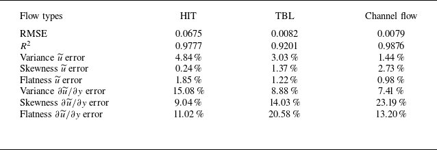
To rigorously assess the cross-domain generalization ability of SoZoGAN, we conduct a comprehensive quantitative evaluation involving multiple types of turbulence, with an SR ratio of 5 in all cases. We consider several accuracy metrics: root-mean-square error (RMSE), coefficient of determination ( $R^2$ ) averaged across all velocity components, and higher-order statistics – up to fourth-order moments – of both velocity fluctuations and gradients (table 2). Across this diverse set of flow cases, SoZoGAN demonstrates remarkable zero-shot transfer performance. The model achieves $R^2$ values close to one, minimal RMSE and errors in the second- to fourth-order moments of velocity consistently below 5 %. Even though the errors for velocity gradient moments are moderately higher (averaging around 14 % for second- to fourth-order moments), they remain well within the acceptable benchmarks established by Buaria & Sreenivasan (Reference Buaria and Sreenivasan2023). It is important to note that Buaria & Sreenivasan (Reference Buaria and Sreenivasan2023) examined only HIT at varying Reynolds numbers. In contrast, our study covers both a broader range of flow types and a wider spectrum of Reynolds numbers, creating a more stringent test of generalization.

Table 2.

Performance metrics of SoZoGAN for turbulence super-resolution in different flow types, with an SR ratio of 5 in all cases.

3.2. Homogeneous turbulence at unseen Reynolds numbers

We assess SoZoGAN’s generalization capability for HIT through zero-shot transfer from the training Reynolds number ( ${\textit{Re}}_\lambda \approx 1200$ ) to an unseen testing condition ( ${\textit{Re}}_\lambda \approx 433$ ). The evaluation dataset comprises 1000 DNS snapshots from the JHTDB at ${\textit{Re}}_\lambda \approx 433$ , where each snapshot provides all three velocity components ( $u$ , $v$ , $w$ ) on a uniform grid. To maintain consistency with pretraining data, we extract $400 \times 400$ planar velocity fields from each snapshot, covering a physical domain of size $2\pi \times 0.5\pi$ in the $(x,y)$ -plane.

Leveraging HIT’s statistical homogeneity, we employ a simplified SoZoGAN variant that operates without zonal decomposition. Model selection is achieved by matching the test case’s Taylor microscale to our library’s precomputed values (figure 1 a). The $1/r \times$ LR input is generated via an average pooling for HR snapshots with a factor of $r$ , preserving large-scale structures while reducing spatial detail.

Figure 3.

Effect of training-testing scale alignment on small-scale HIT generations with SoZoGAN. (a) Low-resolution ( $1/5 \times$ ) input field for the $v$ -velocity component. (b–d) Instantaneous $v$ -component fields generated by SRGANs trained at different Taylor microscales: (b) training scale much larger than testing; (c) testing scale much larger than training; (d) matched scales, compared with (e) HR reference fields. Taylor microscales $\lambda _{\textit{LR}}$ , $\lambda _{\textit{SR}}$ and $\lambda _{\textit{HR}}$ associated with input, reconstructed and DNS reference fields are marked along with the corresponding instantaneous fields. (f) Enlarged views of the boxed regions in (b)–(e) highlight differences in generated vortex structures relative to the HR reference. (g) Wavenumber spectra for all velocity components ( $u, v, w$ ) comparing SoZoGAN generations (aligned case), coarse inputs and DNS references. Here $E_{uu}$ is scaled by $1\times 10^4$ , $E_{vv}$ by $1\times 10^2$ and $E_{ww}$ remains unscaled for clarity. The dash line represents the cutoff wavenumber of the LR input.

To demonstrate the critical role of scale alignment, we systematically evaluate model performance under both matched and mismatched training–testing conditions. Figure 3(b–d) compares instantaneous $v$ -component fields generated by SRGANs trained at different microscales from identical $1/5\times$ LR inputs (figure 3 a), while figure 3(e) shows the corresponding DNS reference. The Taylor microscales, calculated from these velocity fields and indicated in each panel’s upper right-hand corner, are denoted as $\lambda _{\textit{LR}} = 0.5468$ (input), $\lambda _{\textit{SR}}$ (predictions) and $\lambda _{\textit{HR}} = 0.1143$ (DNS reference). The coarse-grained input exhibits an microscale approximately five times larger than the DNS reference (figure 3 e), significantly attenuating small-scale information. When the SRGAN is trained at substantially larger microscales ( $\lambda _{{\textit{train}}} \approx 2\lambda _{{\textit{test}}}$ ), it captures mainly large-scale structures while failing to reconstruct fine details, producing predictions with microscales twice the reference value (figure 3 b). Conversely, models trained at smaller microscales ( $\lambda _{{\textit{train}}} \approx 0.5\lambda _{{\textit{test}}}$ ) generate artificial fine-scale fluctuations, yielding unphysically smaller characteristic scales at the given ${\textit{Re}}_{\lambda }$ . Optimal performance occurs when the microscales of the pretraining and testing data are well aligned (figure 3 d). As highlighted in the enlarged views (figure 3 f) of the boxed regions in figure 3(b–e), SoZoGAN accurately reconstructs small-scale turbulence from $1/5\times$ inputs, with vortical structures closely matching DNS results.

The effect of proper scale alignment is therefore striking: when the microscales in training and testing are matched, SRGAN faithfully reconstructs small-scale turbulent structures, with the predicted microscale remaining within 5 % of the DNS value. This result confirms that scale alignment is essential for producing physically consistent SR. Figure 3(g) further supports this observation by presenting wavenumber spectra for all three velocity components $(u, v, w)$ based on SoZoGAN reconstructions. By comparing these spectra with those of both the LR input and the high-fidelity DNS, it becomes clear that SoZoGAN is able to restore not only the inertial subrange but also dissipation-range spectral content far beyond what is present in the coarse input fields.

3.3. Inhomogeneous turbulence: TBL

Compared with homogeneous turbulence, inhomogeneous wall-bounded turbulence poses a more rigorous challenge for SoZoGAN due to its dramatic variation in characteristic scales along the wall-normal direction. In TBLs, wall shear generates intense small-scale vortices near the wall, while large-scale structures dominate the outer region, where turbulence gradually decays towards laminar conditions. This strong scale heterogeneity highlights the need for adaptive models capable of accurately capturing multiscale features.

3.3.1. Preprocessing of testing data

The testing data here are sourced from a TBL database generated through DNS of incompressible flow over a no-slip flat plate. Detailed descriptions of the computational domain and grid resolutions can be found in the previous studies (Lee & Zaki Reference Lee and Zaki2018). The coordinate system is defined by $x$ , $y$ and $z$ representing the streamwise, wall-normal and cross-flow directions, respectively, with the corresponding velocity components denoted as $u$ , $v$ and $w$ .

The focus of our analysis is a particular two-dimensional cross-plane ( $y{-}z$ plane) at a momentum thickness-based Reynolds number $\textit{Re}_{\theta }\sim 1000$ . From this cross-plane, we extract data for the three velocity components over a size of $y\times z = 23.65L \times 94.6L$ ( $L$ is half-thickness of the plate). The corresponding grid resolution is $400\times 400$ , evenly distributed along each direction. To obtain LR datasets, the HR data are downsampled with the factors of $r=[5,10,16]$ , reducing the grid size to $80\times 80$ , $40\times 40$ and $25\times 25$ , respectively. This reduction is achieved via average pooling for each velocity component (Fukami et al. Reference Fukami, Fukagata and Taira2021a ). To ensure the statistical reliability, 1000 snapshots are collected at equal time intervals over an adequately long period, providing a testing dataset of LR inputs.

Figure 4.

Zonal decomposition and Taylor microscale estimation in TBL SR using SoZoGAN. (a) Hierarchical clustering partitioning the LR TBL domain into three physically meaningful subdomains, with interfaces at $y^+ \approx 102$ and $y^+ \approx 410$ , corresponding to the viscous plus lower log-low, upper log-law and wake regions, respectively. (b) Wall-normal profiles of the estimated Taylor microscale ( $\lambda$ ) predicted by the MLP based on macroscale parameters from LR input, compared with the HR DNS reference.

In the prediction stage, spatial differences in scale distribution should be first identified from the LR field. We perform the zonal decomposition using hierarchical clustering guided by scale-sensitive wavenumber spectra. For the TBL considered, statistical homogeneity in the horizontal directions allows subdomain boundaries to be placed only along the wall-normal direction, simplifying the decomposition process. The number of subdomains is user-defined: increasing it allows finer adaptation to local scale variations and can enhance reconstruction accuracy, but at the cost of requiring a larger library of pretrained SR models. This trade-off will be examined in § 3.3.3. As a representative case, figure 4(a) presents a hierarchical clustering result that partitions the domain into three subdomains, with physical interfaces located at $y^+ \approx 102$ and $y^+ \approx 410$ , where $y^+$ denotes the wall-normal distance normalized by the viscous length scale $\delta _{\nu }$ . These interfaces approximately demarcate (i) viscous plus lower log-low, (ii) upper log-law and (iii) wake region (large-scale motions dominate), reflecting classic boundary layer distribution and demonstrating the physical validity of our zonal decomposition strategy.

After zonal decomposition, the MLP, pretrained on the universal macroscales-to-microscales relationship learned from HIT data, is applied directly to the LR TBL field to estimate the local Taylor microscale ( $\lambda$ ), as illustrated in figure 4(b). Accurate estimation of the Taylor microscale enables scale precalibration, which is critical for scale-oriented SR in inhomogeneous turbulence. At each wall-normal location ( $y^+$ ), the MLP takes as input the macroscale parameters $L$ , $\nu$ and $u^{\prime}$ , all of which are well-preserved and accessible even in coarsened fields. The MLP-estimated wall-normal profile of the Taylor microscale is compared with values obtained from HR DNS, showing close agreement with a low spatially averaged error of $8.28\,\%$ . When spatially averaged over each decomposed subdomain, the estimated $\lambda ^*$ values are 0.0505, 0.1509 and 0.4192 from the near-wall to the outer subdomains, respectively. These averages are used to identify the best-matching microscale indices in the model library, guiding the selection of the appropriate SR models for each individual subdomain.

3.3.2. Roles of zonal scale alignment

We take $5 \times$ SR as our primary case to dissect the roles of microscale alignment and zonal generation within the proposed SoZoGAN framework. To this end, we conduct an ablation study, the results of which are shown in figure 5. Starting from $1/5 \times$ LR inputs (figure 4 a), we compare the instantaneous super-resolved velocity fields for all three components generated by different SRGAN-based approaches against the corresponding DNS reference (figure 5 a) and SRGAN baseline (figure 5 f) snapshots.

Taylor microscale alignment is first evaluated using three SRGAN models pretrained at different scales (figure 5 b–d). Figure 5(b) illustrates the result obtained by applying a sole $5 \times$ SRGAN model, pretrained on HIT samples with a Taylor microscale ( $\lambda _{{\textit{train}}}$ ) approximately twice that of the target TBL test data ( $\lambda _{\textit{TBL}} \sim 0.2321$ , spatially averaged). This model reproduces large-scale turbulence characteristics but fails to resolve the smaller-scale structures near the wall, as it overestimates the relevant microscale features. Conversely, figure 5(c) presents results from an SRGAN model pretrained with a much smaller scale index ( $\lambda _{{\textit{train}}}\approx \ 1/2\lambda _{\textit{TBL}}$ ). Here, the super-resolved fields display pronounced non-physical fluctuations, especially in the $u$ component, indicating that the model has transferred small-scale features inconsistent with the actual microscales of the TBL, thereby generating unrealistic reconstructions. Figure 5(d) demonstrates the effect of applying microscale alignment: a sole $5 \times$ SRGAN model is chosen from the library such that its training microscale matches the spatially averaged $\lambda _{\textit{TBL}}$ of the target field ( $\lambda _{{\textit{train}}}\approx \ \lambda _{{TBL}}$ ). The resulting super-resolved fields exhibit substantially reduced non-physical fluctuations compared with the previous cases and closely match the distributions seen in the DNS reference, as quantified by improved $R^2$ values. This outcome confirms that microscale precalibration enables reliable transfer of turbulence characteristics from HIT data to TBL reconstructions.

Next, we examine how zonal generation enhances reconstruction quality. Figure 5(e) displays results from the full SoZoGAN framework, which combines scale alignment and zonal generation. Compared with the sole scale-aligned model, zonal generation markedly enhances the reproduction of fine velocity fluctuations, especially in the near-wall region (as highlighted in figure 5 f). This improvement is reflected in the accuracy metrics, with $R^2$ reaching nearly 0.9 for $v$ and $w$ and approaching 1 for $u$ . This zonal strategy effectively addresses wall turbulence’s spatial heterogeneity by applying scale-matched models to specific flow subdomains. The study reveals that successful turbulence reconstruction depends on two key elements: first, exact microscale matching to ensure basic physical validity, and second, intelligent zonal decomposition to handle the spatially varying nature of wall turbulence characteristics.

Figure 5.

Effects of microscale alignment and zonal generation and on TBL SR. (a–e) Instantaneous fields of three velocity components (b)–(d) globally generated by SRGANs and (e) zonally generated by SoZoGAN, with $R^2$ values shown below each field. (f) Local zoom-in views of the black dashed boxes shown in (a), (d) and (e), highlighting the generated near-wall small-scale structures of the SRGAN ( $\lambda _{{\textit{train}}}\approx \ \lambda _{\textit{TBL}}$ ) and SoZoGAN, compared with the DNS reference field.

To further assess the quantitative physical fidelity of the super-resolved fields, we examine and compare flow statistics between the generated and reference velocity fields. Figure 6(a) presents wall-normal profiles of the normalized turbulence intensities, $\sigma _u(y)/U_{\textit{a}v\textit{g}}(y)$ , $\sigma _v(y)/U_{\textit{a}v\textit{g}}(y)$ and $\sigma _w(y)/U_{\textit{a}v\textit{g}}(y)$ , obtained by averaging over 1000 snapshots. The proposed SoZoGAN framework closely reproduces the DNS reference profiles, accurately capturing the pronounced turbulence intensities near the wall that are absent in the coarse input fields. In contrast, the non-zonal baseline SRGAN presents substantial discrepancies across the viscous sublayer, buffer layer and logarithmic region, failing to reconstruct the correct levels of turbulence intensity.

To provide a more direct assessment of microscale structure generation, we analyse the wall-normal profiles of the Taylor microscale length presented in figure 6(b). The SoZoGAN, equipped with zonal generation, achieves excellent agreement with the DNS reference in the critical near-wall region ( $y^+ \approx 0$ – $150$ ), faithfully capturing the true eddy sizes. In contrast, the non-zonal baseline SRGAN systematically overestimates the Taylor microscales in this region. These findings underscore the effectiveness of SoZoGAN’s zonal decomposition, which enables not only accurate reproduction of turbulent intensities but also precise recovery of average microscale eddy sizes, particularly in the most challenging near-wall portion of the wall-bounded turbulence.

Figure 6.

Wall-normal profiles of (a) turbulent intensities and (b) Taylor length scales for global and zonal generation, both with microscale alignment; error bars show standard deviations at each wall distance.

Furthermore, we examined the spatial continuity of the generated TBL field across subdomain interfaces by evaluating wall-normal profiles of the streamwise-velocity gradient $(\partial u/\partial y)$ (figure 7 a) and the Reynolds-stress components $\overline {u^{\prime}u^{\prime}}$ , $\overline {u^{\prime}v^{\prime}}$ and $\overline {v^{\prime}v^{\prime}}$ (figure 7 b). These profiles, covering the full wall-normal range and all decomposed subdomains, agree closely with DNS and remain smooth across interface locations, with no discernible jumps or spurious fluctuations. Combined with the turbulence intensity and Taylor microscale distributions shown in figure 6, which likewise exhibit seamless behaviour at interfaces, these results confirm that SoZoGAN’s zonal generation strategy, together with the $1\times$ SRGAN smoothing step (figure 1 c), produces a globally continuous and physically consistent super-resolved flow field.

Figure 7.

Wall-normal profiles of (a) vertical gradient of streamwise velocity, $\partial u / \partial y$ , and (b) the Reynolds stress components, $\overline {u^{\prime}u^{\prime}}$ , $\overline {u^{\prime}v^{\prime}}$ and $\overline {v^{\prime}v^{\prime}}$ , spanning the wall-normal range across all decomposed subdomains (labelled by A, B and C).

We finally investigate the turbulent energy distribution of the generated small-scale structures within the TBL to highlight SoZoGAN’s local spectral performance. Figure 8 presents the horizontal wavenumber spectra at two representative wall-normal locations, computed over 1000 test snapshots. In the near-wall region ( $y^+ \approx 30$ ), as shown in figure 8(a), SoZoGAN more accurately captures the energy cascade across the high-wavenumber range, clearly outperforming the baseline SRGAN model pretrained with an average characteristic microscale ( $\lambda _{\textit{train}}\approx \lambda _{\textit{TBL}}$ ). This advantage arises because the baseline model’s learned characteristic microscale tends to exceed the scales present near the wall. At higher wall-normal locations, closer to the free stream ( $y^+ \approx 500$ ; figure 8 b), SoZoGAN successfully avoids the overestimation of microscale turbulence energy. Such overprediction is a known limitation of the conventional sole-model approach, where the learned scale underestimates the actual eddy sizes farther from the wall. This comparison underscores SoZoGAN’s adaptive capacity to resolve spatially varying scales, significantly enhancing the spectral fidelity of the generated microscale turbulence throughout the distinct subregions of the TBL.

Figure 8.

Wavenumber spectra for the three velocity components, calculated at certain heights of (a) $y^+\approx 30$ (near the wall) and (b) $y^+\approx 500$ (far away from the wall), comparing SoZoGAN and SRGAN. Here $E_{uu}$ is scaled by $1\times 10^6$ , $E_{vv}$ by $1\times 10^3$ and $E_{ww}$ remains unscaled for clarity.

3.3.3. Robustness with respect to subdomain partitioning and SR ratio

We investigate how the number of subdomains affects multiscale turbulence generation accuracy and the framework’s applicable SR ratios, as shown in figures 9 and 10, respectively.

Figure 9.

Effect of the partitioning number on the SoZoGAN performance in TBL: (a) synthesized instantaneous $v$ fields along with their corresponding (b) wavenumber spectra, using SoZoGAN based on two, three and five partitioning subdomains.

Figure 9 examines the impact of varying the number of decomposed subdomains on the accuracy of multiscale turbulence generation. The TBL SR using SoZoGAN are carried out with two, three and five subdomains. As shown in figure 9(a), the instantaneous super-resolved velocity fields produced with two subdomains exhibit larger generation errors than those with three subdomains. Increasing the partitioning from two to three subdomains reduces the RMSE by approximately 50 %, indicating a clear gain from finer zonal decomposition. By contrast, increasing the number from three to five subdomains produces only minor improvements in both the RMSE and $R^2$ metrics.

The corresponding wavenumber spectra at $y^+ \approx 500$ are presented in figure 9(b). In the two-subdomain case, the energy in the dissipation range is markedly overestimated relative to the DNS reference. This overestimation is substantially reduced when three subdomains are used, owing to a more accurate estimation of characteristic turbulent scales in the outer-layer wake region. Improved scale estimation suppresses the introduction of spurious high-frequency fluctuations during reconstruction. Further increasing the number of subdomains beyond three yields only modest spectral improvements while significantly increasing model complexity and computational cost.

Collectively, the three-subdomain configuration achieves a strong balance between reconstruction accuracy and computational efficiency. It captures the wall-normal variation of characteristic scales well enough to prevent spectral distortions, while avoiding the diminishing returns and extra cost in data preparation and model training that come with finer partitioning beyond three subdomains.

Figure 10.

Effect of the coarseness of the LR inputs on the SoZoGAN performance in TBL: (a) synthesized instantaneous $v$ fields and (b) cross-correlation coefficient contours of predicted snapshots from the $1/5\times$ , $1/10\times$ and $1/16\times$ LR inputs.

We further evaluate the applicability of the proposed SoZoGAN framework for TBL generation across a range of SR ratios ( $r$ ). As illustrated in figure 10(a), instantaneous fields are reconstructed from $1/5 \times$ , $1/10 \times$ and $1/16 \times$ LR inputs using $r \times$ SoZoGAN ( $r=[5,10,16]$ ). For $r = 5$ and $10$ , SoZoGAN effectively reproduces the near-wall microscale vortex structures, maintaining consistently low RMSE values and near-unity $R^2$ values, indicative of excellent agreement with DNS references. When the ratio increases to $r = 16$ , SoZoGAN still captures the major flow patterns present in the DNS fields, despite the much coarser input resolution. However, the recovery of near-wall microscale structures diminishes, both in terms of their number and intensity. This limitation is reflected in a marked increase in RMSE and a noticeable decline in $R^2$ , underscoring the greater challenge of recovering fine-scale features at higher SR ratios.

To probe the spatial structures of the SoZoGAN-generated fields, figure 10(b) presents the spatial cross-correlation coefficients $R_{vv}(\Delta y^+,\Delta z^+)$ for wall-normal velocity at different SR ratios. Across all ratios examined, the reconstructed fields yield correlation patterns largely consistent with DNS. Nevertheless, as $r$ increases, the absolute values of these coefficients tend to be slightly overestimated, reflecting a loss of spatial complexity due to the underrepresentation of microscale structures in the generated fields.

Overall, these results confirm the robustness and accuracy of SoZoGAN in generating microscale turbulence for SR ratios up to $r=10$ . Even at $r=16$ , the framework preserves the fundamental spatial characteristics of HR wall turbulence, albeit with some loss of detail. Beyond this ratio, individual SRGAN models within the SoZoGAN framework reach their capacity limits of SR, and increasing the number of subdomains alone does not yield further improvements in predictive accuracy.

3.4. Inhomogeneous turbulence: turbulent channel flow

The next application focuses on the SR generation of a turbulent channel flow with a friction Reynolds number of $\textit{Re}_{\tau }= 1000$ (Lee, Malaya & Moser Reference Lee, Malaya and Moser2013). Similar to the TBL, the turbulent channel flow is wall-bounded and exhibits significant scale variation in the wall-normal direction. However, there are important distinctions between the two types of turbulence.

In the outer region (far from the wall) of the TBL, turbulence tends to become smoother and less intense, with velocity fluctuations weakening as the distance from the wall increases. In contrast, turbulence in the channel flow remains relatively active and exhibits significant spatial fluctuations even far from the walls. This is primarily due to the confinement imposed by the two parallel walls, which restricts the dissipation of turbulent energy. As a result, super-resolving turbulent channel flow presents a unique challenge.

3.4.1. ‘Zero-shot’ small-scale generation using SoZoGAN

For this test case, the velocity data of the turbulent channel flow are also obtained from a DNS database provided by JHTDB. The coordinate system and corresponding velocity components adhere to the definitions used in the TBL database. To focus on the generation of wall turbulence, the data are extracted from a $y{-}z$ section near one of the channel walls. The section is $y\times z$ = 0.3835 $H$ $\times$ 1.5340 $H$ with $500 \times 500$ evenly distributed grid nodes, where $H$ is the channel height. To obtain the LR inputs, the original DNS fields are downsampled to $50\times 50$ using a factor of 10. A total of 1000 snapshots are selected, evenly distributed across the entire duration of the simulation, ensuring a broad statistical representation of the turbulence.

Subdomains are identified using hierarchical clustering based on the wavenumber spectra of LR inputs. The corresponding estimated Taylor microscales, obtained via a MLP, are shown in figure 11(a). Owing to the similar generation mechanisms governing wall-bounded turbulence in both the TBL and channel flow, the same procedures for zonal decomposition and microscale estimation are employed. These procedures effectively capture both the magnitude and the wall-normal variation of microscales in the DNS reference, resulting in a low spatially averaged error ( $1.72\,\%$ ). Across the channel, three distinct scale-related subdomains emerge: quasilinear, transitional and stable subdomains.

Figure 11.

‘Zero-shot’ generation of vertical $y$ – $z$ plane in turbulent channel flow by the proposed SoZoGAN. (a) Zonal decomposition and microscale estimation of the turbulent channel flow. Three scale-related subdomains are decomposed. Taylor microscale estimation is performed along the wall-normal direction of the turbulent channel flow. (b) Generated instantaneous fields of three velocity components with their reconstruction errors (RMSE) and accuracies ( $R^2$ ). The green dashed lines shown on the LR inputs (ii) represent the subdomain boundaries identified using hierarchical clustering.

After zonal decomposition and microscale estimation, we perform the scale-oriented generation of small-scale channel flow. As depicted in figure 11(b), the synthesized $u$ , $v$ and $w$ velocity fields exhibit agreement with the DNS results. The large spatial fluctuations away from the wall are well replicated through the ‘zero-shot’ transfer of the SoZoGAN framework. The RMSE errors are low and the $R^2$ accuracies all exceed 0.9, indicating that the SoZoGAN generation accurately captures the multiscale turbulent structures.

To further assess the generality and Galilean invariance of SoZoGAN, we conducted additional tests on horizontal $x$ – $z$ planes of channel flow at two wall distances: $y^+ \approx 30$ (near-wall region) and $y^+ \approx 300$ (outer-layer region). These planes were extracted from the same DNS database. Figures 12(a) and 12(b) present the instantaneous total velocity $U$ fields generated in a zero-shot manner, while figure 12(c) shows the corresponding wavenumber spectra for both wall distances. In the near-wall case (figure 12 a), which is characterized by pronounced streak-like structures, SoZoGAN faithfully reproduces the fine-scale velocity fluctuations observed in the DNS reference, achieving $R^2$ values close to 0.9 despite the complexity of the flow. In the outer-layer case (figure 12 b), where the turbulent structures are significantly larger in scale and more isotropic, the generated fields exhibit similarly high agreement with the DNS data and preserve the spatial organization of coherent motions.

The microscale alignment in SoZoGAN plays a key role in distinguishing scale-specific features at different wall distances. Smaller near-wall scales and larger outer-layer structures are both accurately recovered without any additional training. The wavenumber spectra further confirm that SoZoGAN reproduces the inertial-subrange energy characteristics appropriate to each wall distance (figure 12 c). Consistent reconstruction performance across both $x$ – $y$ and $x$ – $z$ cross-planes, and at wall distances with notably different turbulent scales, provides strong evidence that the SoZoGAN satisfies Galilean invariance. This invariance implies that the same pretrained generative models can be applied in uniformly translating reference frames without loss of reconstruction fidelity.

Figure 12.

‘Zero-shot’ generation of horizontal $x$ – $z$ planes in turbulent channel flow by the proposed SoZoGAN. Instantaneous total velocity $U$ fields at two wall distances, (a) $y^+ \approx 30$ (near-wall region) and (b) $y^+ \approx 300$ (outer-layer region), reconstructed at 10 $\times$ SR from LR inputs. Their reconstruction errors (RMSE) and accuracies ( $R^2$ ) are marked. (c) Wavenumber spectra of the reconstructed $U$ distributions for both wall distances.

3.4.2. ‘Zero-shot’ performance of SoZoGAN versus other state-of-the-art models

We examine the performance of SoZoGAN in comparison with several state-of-the-art SR models for microscale turbulence generation in channel flow. The baseline models include hDSC-MS, a deterministic approach that incorporates multiscale modelling to capture both large and small-scale turbulent structures (Du et al. Reference Du, Qu, He and Guo2018; Fukami et al. Reference Fukami, Fukagata and Taira2019). In addition, two generative models are considered: diffusion (Shu, Li & Barati Farimani Reference Shu, Li and Barati Farimani2023), which employs a progressive denoising framework to iteratively refine coarse inputs by learning the conditional score function of turbulence statistics, and SRGAN, which serves as the base SR model embedded within SoZoGAN. Unlike SoZoGAN, all baseline models do not incorporate zonal decomposition or scale alignment. Instead, they are trained on original HIT samples ( $\lambda _1^{\prime} \sim 0.0331$ ) and directly transferred, without fine-tuning, to the channel flow scenario for small-scale generation.

Figure 13(a) presents a comparative analysis of instantaneous streamwise velocity fields generated by these models. The hDSC-MS model fails to resolve many critical fine-scale features, resulting in excessively smoothed fields that lack the distinctive small-scale vortical details characteristic of near-wall turbulence. Meanwhile, the generative diffusion and SRGAN models introduce spurious, non-physical fluctuations – a consequence of inadequate calibration to local turbulent scales and limited adaptability to the heterogeneity of wall-bounded flows. In sharp distinction, SoZoGAN faithfully reconstructs the complex scale variation observed across the wall-normal direction in channel flow. It accurately recovers intricate small-scale roll-up structures near the wall, while smoothly transitioning to larger-scale features farther from the wall, yielding instantaneous velocity fields in close agreement with DNS.

The superiority of SoZoGAN is expected to be underscored in the wavenumber spectra comparison. In figure 13(b), the wavenumber spectra of three velocity components averaged over the region of $y^+\lt 400$ . The spectra produced by SoZoGAN most closely match DNS results across the entire range of wavenumbers. The hDSC-MS underestimates turbulence energy at small scales, reflecting its limited microscale reconstruction capability. While diffusion achieves reasonable small-scale energy recovery, it fails to preserve energy in the inertial subrange, indicating inconsistent multiscale turbulence generation. The SRGAN, on the other hand, maintains reasonable accuracy in the inertial subregion but tends to overpredict turbulence energy at the finest scales. Overall, these results underscore that the scale-oriented zonal decomposition and microscale alignment strategies of SoZoGAN provide critical advantages for robust and accurate microscale turbulence generation in wall-bounded flows.

Despite the need to pretrain multiple specialized SRGANs, the total training cost of SoZoGAN remains moderate (approximately 18 GPU-hours on two NVIDIA Tesla V100 GPUs) and is a one-time offline investment. Inference of SoZoGAN is somewhat slower than the baselines due to the zonal generation and subdomain merging procedures; however, for the channel flow case reported here, the average inference time per snapshot is only approximately 0.075 s on the same hardware. These computational demands are well within practical limits and are more than offset by the gains in multiscale generation accuracy and robustness.

Figure 13.

Comparison of ‘zero-shot’ generation for microscale turbulent channel flow using different SR models: (a) instantaneous streamwise velocity fields and (b) wavenumber spectra of three velocity components averaged over the region of $y^+\lt 400$ predicted by hDSC-MS, diffusion, SRGAN and SoZoGAN, compared with the DNS reference.

3.5. Evaluations of zero-shot transfer in SoZoGAN

To emphasize the effectiveness of the proposed zero-shot transfer strategy, we introduce an ‘in-domain model’ baseline. This baseline uses an SRGAN with exactly the same network architecture, loss function and hyperparameter settings as those SRGANs employed in SoZoGAN. The key difference lies in the training set-up: (i) ‘in-domain model’ – trained and tested entirely within the same flow type using a standard train–test split from its DNS dataset; (ii) ‘cross-domain model’ – operates in a zero-shot, cross-domain setting, with each SRGAN pretrained once on a single HIT dataset and applied without retraining or fine-tuning to generate SR fields for completely unseen target flows, including HIT at different Reynolds numbers and spatially inhomogeneous turbulence. This comparison contrasts an idealized best-case scenario with abundant target-flow data (‘in-domain model’) against the more challenging and practically relevant zero-shot inference task (‘cross-domain model’) addressed by SoZoGAN.

Figure 14 compares turbulence-generation results for both HIT and TBL cases. In HIT, the instantaneous $v$ -component fields produced by SoZoGAN (figure 14 a) are visually and statistically indistinguishable from both the DNS reference (figure 14 c) and the ‘in-domain model’ output (figure 14 b). The Taylor microscales $\lambda _{\textit{SR}}$ and $\lambda _{\textit{HR}}$ derived from SoZoGAN, the ‘in-domain model’ and DNS data exhibit excellent agreement, confirming the accurate reproduction of key small-scale structures in isotropic turbulence. In TBL, SoZoGAN likewise generates instantaneous structures in close agreement with both DNS (figure 14 f) and the ‘in-domain model’ (figure 14 e), while its scale-oriented zonal generation strategy captures the wall-normal variation of characteristic turbulent scales more faithfully. This improvement results in a modest increase in $R^2$ accuracy over the ‘in-domain model’, underscoring the benefit of localized scale-aware generation in wall-bounded flows.

Overall, these results demonstrate that even in the zero-shot ‘cross-domain model’ setting, SoZoGAN achieves turbulence-generation accuracy comparable to the ‘in-domain model’ trained directly on target-flow data. This confirms the effectiveness of the proposed method and demonstrates that high fidelity turbulence generations are possible with substantially reduced data requirements. Operating without any HR target flow training data makes SoZoGAN particularly valuable in scenarios where such data are scarce or unavailable, while still preserving the physical consistency of the reconstructed fields.

Figure 14.

Effectiveness of zero-shot transfer in SoZoGAN. (a–c) Small-scale HIT generations: instantaneous $v$ -component fields from (a) SoZoGAN (‘cross-domain model’), (b) SRGAN baseline (‘in-domain model’) trained directly on target HIT data and (c) DNS reference. Reported $\lambda _{\textit{SR}}$ and $\lambda _{\textit{HR}}$ indicate the Taylor microscales associated with reconstructed and DNS fields. (d–f) Small-scale TBL generations: instantaneous $v$ -component fields from (d) SoZoGAN, (e) SRGAN baseline trained directly on target TBL data and (f) DNS reference. The $R^2$ value shown over each generated field is averaged across the generated $u$ , $v$ and $w$ fields.

3.6. Discussions on mechanisms of SoZoGAN generalization

The reason for this robust generalization finds its explanation in the foundations of turbulence theory. The SoZoGAN can transfer effectively across very different turbulence regimes, thanks in large part to Kolmogorov’s local isotropy hypothesis (Kolmogorov Reference Kolmogorov1941). This hypothesis suggests that the small-scale statistics of turbulence are nearly universal and largely independent of the large-scale anisotropy of the flow. Empirical evidence from previous spectral analyses and second-order statistical studies (Saddoughi & Veeravalli Reference Saddoughi and Veeravalli1994; Shen & Warhaft Reference Shen and Warhaft2000) supports the idea that small-scale turbulence features are sufficiently generic. This means that models pretrained on HIT can be reasonably extended to more complex, strongly sheared flows. In addition, SoZoGAN’s loss function incorporates a physical constraint – the residual of the incompressible continuity equation – which further aids adaptation to flows with pronounced anisotropy and strong shear. Our results confirm that SoZoGAN sustains high accuracy, not only for velocity spectra but also for higher-order velocity moments (up to fourth order) over a wide range of turbulence scenarios.

The model’s strong performance in representing the statistics of small-scale turbulent motions is evident in its agreement with DNS for both velocity fields and low-order velocity gradient moments (see table 2). For many engineering and geophysical applications, this level of accuracy is sufficient. Nevertheless, persistent small-scale anisotropy – especially in wall-bounded flows with prominent mean shear (Shen & Warhaft Reference Shen and Warhaft2000) – remains a challenge for transfer learning based solely on HIT data. In these cases, third- and fourth-order velocity gradient moments show an average error of approximately 18 %. This highlights the inherent limitation of capturing subtle features of small-scale anisotropy using HIT-pretrained models. Future studies might overcome this limitation by explicitly modelling the effects of shear and intermittency (Shen & Warhaft Reference Shen and Warhaft2000; Buaria & Pumir Reference Buaria and Pumir2025), with special attention to the fine-scale moments that are critical in near-wall regions for momentum and scalar transport.

3.7. Adjustment of SoZoGAN to adapt to energy-filtered coarse inputs

The scale-oriented zonal framework proposed in this study is architecture-agnostic, and can readily extend beyond GANs (SoZoGAN) to other deep learning SR models. This flexibility further broadens its applicability to diverse turbulence reconstruction scenarios. In particular, in practical numerical simulations with extremely coarse grids, the resulting LR data may exhibit premature or excessive attenuation of TKE due to strong numerical dissipation. Such cases deviate from the moderate downsampling regime considered for the SoZoGAN discussed in previous sections, where the LR inputs are generated through well-controlled average pooling that preserves energy in the energy-containing motions and part of the inertial subrange.

To address these highly energy-filtered LR inputs, the EC-SRGAN proposed by Wu et al. (Reference Wu, Zhang, Zhou, Chen, Han and Cao2024) can be embedded within the present scale-oriented zonal framework, yielding a hybrid model referred to here as SoZoEC–SRGAN (a variant of SoZoGAN). In the approach of Wu et al. (Reference Wu, Zhang, Zhou, Chen, Han and Cao2024), the LR fields are first obtained by average-pooling from DNS turbulent fields, followed by a low-pass filtering step. This additional filtering mimics the enhanced energy dissipation in the energy-containing range and inertial subrange observed in very coarse-grid simulations. In our hybrid integration, the GAN component of SoZoGAN is replaced by EC-SRGAN, whose architecture and loss functions were designed specifically to compensate for such energy deficits and recover fine-scale turbulent motions in wall-bounded flows from strongly energy-filtered inputs.

As a representative demonstration, we apply SoZoEC–SRGAN to a turbulent channel flow case with LR input fields exhibiting severe energy loss, corresponding to a $10\times$ SR task. Figure 15(a) compares instantaneous fields of the three velocity components from the energy-filtered LR inputs, the SoZoEC–SRGAN reconstructions and the HR DNS references. The SoZoEC–SRGAN outputs successfully recover spatially coherent near-wall fine-scale structures that are largely absent in the LR input, with flow features and spatial distributions closely matching those in the DNS fields. Figure 15(b) presents the corresponding wavenumber spectra, showing that SoZoEC–SRGAN effectively restores energy in the lower part of the inertial subrange and extends the $-5/3$ energy cascade towards finer scales. This indicates that SoZoEC–SRGAN can reconstruct statistically accurate small-scale turbulence contents despite substantial energy deficits in the coarse inputs.

Figure 15.

‘Zero-shot’ generation of turbulent channel flow from strongly energy filtered LR inputs using the proposed SoZoEC–SRGAN. (a) Instantaneous fields of the three velocity components, comparing LR inputs obtained by average pooling and subsequent low pass filtering of DNS data, $10\times$ super-resolved outputs from SoZoEC–SRGAN, and the DNS reference fields. (b) Corresponding wavenumber spectra of three velocity components for the LR inputs, super-resolved outputs and DNS references.

This example illustrates that the proposed scale-oriented zonal framework can adaptively incorporate SR models with complementary strengths to target specific deficiencies in the input data. In particular, by selecting or integrating architectures capable of compensating for energy loss, the framework extends the applicability of zero-shot turbulence SR to extreme coarse-grid scenarios in numerical settings.

3.8. Discussions on limitations of SoZoGAN

The effectiveness of turbulence SR with SoZoGAN is fundamentally governed by the relationship between input grid resolution (the smallest resolvable turbulence scale in input data) and the characteristic length scales of turbulence. A key challenge lies in ensuring that the coarse input grid is sufficiently fine to retain the information needed for accurate recovery of small-scale structures. Through systematic analysis of homogeneous turbulence reconstruction (summarized in figure 16), we identify a distinct resolution threshold that determines the feasibility of SR.

Figure 16(a) quantifies SoZoGAN performance across varying degrees of input coarsening using the coefficient of determination,

(3.1)

\begin{equation} R^2 = \frac {1}{n} \sum _{j=1}^{n} \left [ 1 - \frac {\sum _{i=1}^{m}(y_{{\textit{HR}},i} - y_{{ SR},i})^2}{\sum _{i=1}^{m}(y_{{\textit{HR}},i} - \bar {y}_i)^2} \right ]\!, \end{equation}

where $y_{\textit{HR}},{\textit {i}}$ is the DNS reference velocity at the $i$ th grid point, $y_{\textit{SR}},{\textit {i}}$ is the predicted velocity, $\bar {y}_i$ is the DNS mean at that grid point and $m$ , $n$ denote the number of grid points and snapshots. Note that $\lambda _{\textit{HR}}$ represents the Taylor microscale calculated from the DNS reference field. When the coarse grid spacing is below approximately $1.1\lambda _{\textit{HR}}$ ( $1/8 \times$ LR input), SoZoGAN achieves high predictive accuracy ( $R^2 \gt 0.9$ ), producing small-scale turbulence that is both visually and physically credible. However, as the grid spacing increases beyond $1.4\lambda _{\textit{HR}}$ ( $1/10 \times$ LR input), the ability to recover fine-scale features diminishes rapidly. This deterioration in performance is closely tied to the coarse input’s capacity to retain large-scale flow features and support precise estimation of the microscale, as shown in figure 16(b). For input grids no coarser than $1.1\lambda _{\textit{HR}}$ , the integral scale $L_{\textit{LR}}$ deviates from the DNS benchmark $L_{\textit{HR}}$ by less than $16\,\%$ , and the MLP predicts the microscale $\lambda ^*$ with an average error of only $7.8\,\%$ . In this regime, SoZoGAN reconstructs fields whose microscale $\lambda _{\textit{SR}}$ is close to the DNS reference with just $8.2\,\%$ error, indicating acceptable physical consistency. When the grid spacing exceeds $1.4\lambda _{\textit{HR}}$ , however, $L_{\textit{LR}}$ deviates by more than $25\,\%$ and $\lambda ^*$ is substantially overestimated, producing SoZoGAN-generated fields with $\lambda _{\textit{SR}}$ more than $27\,\%$ larger than the DNS value. Such deviations significantly undermine the physical fidelity of the reconstructed turbulence.

Figure 16.

Robustness of turbulence SR to input coarsening with SoZoGAN. (a) Accuracy of the super-resolved velocity fields, quantified by the coefficient of determination ( $R^2$ ), as a function of the downsampling factor. (b) Predicted Taylor microscales of the SoZoGAN output ( $\lambda _{\textit{SR}}$ ), MLP-estimated Taylor microscales from coarse inputs ( $\lambda ^*$ ) and corresponding input integral scales ( $L_{\textit{LR}}$ ) at varying levels of input coarsening. The blue and black dash lines represent the calculated Taylor and integral scales based on the HR reference fields, respectively. These results reveal the critical threshold in input resolution required for reliable small-scale reconstruction.

The interplay between input resolution and recoverable turbulence scales suggests a practical strategy for computational fluid dynamics. Suppose one wishes to generate turbulence with a target Taylor microscale $\lambda _{\textit{HR}}$ . In this case, a rapid numerical simulation can be performed using a grid with a spacing of approximately $1.1 \lambda _{\textit{HR}}$ to produce a coarse flow field. This field then serves as input to SoZoGAN, which reconstructs the corresponding fine-scale turbulent features both efficiently and accurately. Such an approach greatly accelerates turbulence generation and offers a promising new pathway for computational fluid dynamics simulations.

Our findings also crystallize two main guidelines for applying the SoZoGAN framework. First, as discussed above, it is crucial to preserve information about the macroscale structures in the coarse input. If the grid becomes too coarse to resolve these structures, accurate prediction of small-scale turbulence is no longer feasible.

Second, the Taylor-scale Reynolds number ${\textit{Re}}_\lambda$ present in the pretraining HIT dataset should reach at least as large as those in the testing turbulence. The flip between the training and testing ${\textit{Re}}_\lambda$ might lead to incorrect generated turbulence. Recent work (Fukami, Goto & Taira Reference Fukami, Goto and Taira2024; Yeo et al. Reference Yeo, Zimoń, Zayats and Zhuk2024) confirms that models trained at lower ${\textit{Re}}_\lambda$ fail to reconstruct the small-scale features of higher ${\textit{Re}}_\lambda$ flows. This is because higher ${\textit{Re}}_\lambda$ turbulence exhibits broader distributions of velocity gradient invariants (Q–R space) than lower- ${\textit{Re}}_\lambda$ data can capture. Consequently, models trained on lower ${\textit{Re}}_\lambda$ must extrapolate beyond their training range when applied to higher- ${\textit{Re}}_\lambda$ flows, resulting in underprediction of scale-invariant turbulent features. In this work, high-to-low ${\textit{Re}}_\lambda$ transfer is achieved by scaling up the original HIT field to create training samples with larger characteristic scales, improving compatibility with lower- ${\textit{Re}}_\lambda$ SR targets. Conversely, a ‘scaling-down’ approach could be used to emulate scale-invariant features characteristic of high- ${\textit{Re}}_\lambda$ flows, enriching low- ${\textit{Re}}_\lambda$ datasets and potentially enhancing low-to-high ${\textit{Re}}_\lambda$ generalization. This will be explored in future work.

Finally, although SoZoGAN in this paper employs subdomain decomposition only along the wall-normal direction, the method is readily extendable to more localized partitioning, as demonstrated in figure 2(b). While the current implementation uses regular rectangular subregions for convolutional processing, it can be straightforwardly generalized to adaptively defined subdomains that more effectively capture the complex spatial variations present in real turbulent flows (Fukami et al. Reference Fukami, Maulik, Ramachandra, Fukagata and Taira2021b ). By selecting appropriate partitioning strategies, the SoZoGAN framework is flexible enough to accommodate a wide range of flow inhomogeneities and geometric configurations.

4. Conclusions

This study proposes SoZoGAN, a novel framework for efficient, high-fidelity turbulence SR that generalizes across diverse flow types using only coarse-grained inputs. Unlike conventional data-intensive methods, SoZoGAN leverages pretraining on a single, readily available HIT dataset. Through strategically designed scaling transformations of HIT data, the framework constructs a library of scale-specific SRGAN models, enabling comprehensive coverage of turbulent scales.

A central feature of SoZoGAN is its capability to exploit the universality of small-scale turbulence dynamics. This allows for robust ‘zero-shot’ generation of turbulence across previously unseen flow scenarios, including not only HIT but also boundary layer and channel flow distinct from the training data. Another key innovation is the zonal decomposition strategy, which leverages local, scale-sensitive physical quantities to guide the partitioning of input fields. This approach addresses the inherent spatial heterogeneity of turbulent flows and enhances the model’s adaptability to complex, non-homogenous turbulent structures. Compared with existing state-of-the-art turbulence SR models, SoZoGAN demonstrates distinct advantages in two crucial aspects: the physical fidelity of small-scale turbulence reconstruction and adaptability to spatially heterogeneous flows. Moreover, the scale-oriented and architecture-agnostic design of SoZoGAN ensures compatibility with a wide range of deep learning models beyond GAN-based networks, offering the potential for further methodological innovation. Overall, SoZoGAN sets a new benchmark for turbulence SR, providing an efficient, generalizable, and physically consistent platform for advancing turbulence modelling in computational fluid dynamics.

Funding

This study was supported by the National Natural Science Foundation of China (52478535), the National Key R&D Program of China (2023YFE0120000), the Natural Science Foundation of Chongqing (CSTB2023NSCQ-MSX0060), the Future Foundation of the Energy Science (WLNY-MS-2022–014) and Guangdong Basic and Applied Basic Research Foundation (2024A1515240081).

Declaration of interests

The authors report no conflict of interest.

Code availability

Sample codes for constituting and training our SoZoGAN framework are available at https://github.com/HookGoh/Tur-SRGANs.git.

Footnotes

†

These authors contributed equally to this work.

References

Aluie, H. 2009 Hydrodynamic and magnetohydrodynamic turbulence: invariants, cascades, and locality. PhD thesis, The Johns Hopkins University, Baltimore.CrossRef Google Scholar

Benzi, R., Ciliberto, S., Tripiccione, R., Baudet, C., Massaioli, F. & Succi, S. 1993 Extended self-similarity in turbulent flows. Phys. Rev. E 48, R29.CrossRef Google Scholar PubMed

Brunton, S.L., Noack, B.R. & Koumoutsakos, P. 2020 Machine learning for fluid mechanics. Annu. Rev. Fluid Mech. 52, 477–508.CrossRef Google Scholar

Buaria, D., Clay, M.P., Sreenivasan, K.R. & Yeung, P.K. 2021 Small-scale isotropy and ramp-cliff structures in scalar turbulence. Phys. Rev. Lett. 126, 034504.CrossRef Google Scholar PubMed

Buaria, D. & Pumir, A. 2025 Universality of extreme events in turbulent flows. Phys. Rev. Fluids 10, L042601.CrossRef Google Scholar

Buaria, D. & Sreenivasan, K.R. 2023 Forecasting small-scale dynamics of fluid turbulence using deep neural networks. Proc. Natl Acad. Sci. USA 120 (30), e2305765120.CrossRef Google Scholar PubMed

Cao, N., Chen, S. & Doolen, G.D. 1999 Statistics and structures of pressure in isotropic turbulence. Phys. Fluids 11 (8), 2235–2250.CrossRef Google Scholar

Cao, Y., Tamura, T., Zhou, D., Bao, Y. & Han, Z. 2022 Topological description of near-wall flows around a surface-mounted square cylinder at high Reynolds numbers. J. Fluid Mech. 933, A39.CrossRef Google Scholar

Choi, H. & Moin, P. 2012 Grid-point requirements for large eddy simulation: Chapman’s estimates revisited. Phys. Fluids 24, 011702.CrossRef Google Scholar

Cuéllar, A., Güemes, A., Ianiro, A., Flores, Ó., Vinuesa, R. & Discetti, S. 2024 Three-dimensional generative adversarial networks for turbulent flow estimation from wall measurements. J. Fluid Mech. 991, A1.CrossRef Google Scholar

Dhariwal, P. & Nichol, A. 2021 Diffusion models beat gans on image synthesis. Adv. Neur. In 34, 8780–8794.Google Scholar

Du, P., Parikh, M.H., Fan, X., Liu, XY. & Wang, JX. 2024 Conditional neural field latent diffusion model for generating spatiotemporal turbulence. Nat. Commun. 15, 10416.CrossRef Google Scholar PubMed

Du, X., Qu, X., He, Y. & Guo, D. 2018 Single image super-resolution based on multi-scale competitive convolutional neural network. Sensors 18 (3), 789.CrossRef Google Scholar PubMed

Dunbar, D., van der A, D.A., Scandura, P. & O’Donoghue, T. 2023 An experimental and numerical study of turbulent oscillatory flow over an irregular rough wall. J. Fluid Mech. 955, A33.CrossRef Google Scholar

Fukami, K., Fukagata, K. & Taira, K. 2019 Super-resolution reconstruction of turbulent flows with machine learning. J. Fluid Mech. 870, 106–120.CrossRef Google Scholar

Fukami, K., Fukagata, K. & Taira, K. 2021 a Machine-learning-based spatio-temporal super resolution reconstruction of turbulent flows. J. Fluid Mech. 909, A9.CrossRef Google Scholar

Fukami, K., Fukagata, K. & Taira, K. 2023 Super-resolution analysis via machine learning: a survey for fluid flows. Theor. Comput. Fluid Dyn. 37, 421–444.CrossRef Google Scholar

Fukami, K., Goto, S. & Taira, K. 2024 Data-driven nonlinear turbulent flow scaling with Buckingham Pi variables. J. Fluid Mech. 984, R4.CrossRef Google Scholar

Fukami, K., Maulik, R., Ramachandra, N., Fukagata, K. & Taira, K. 2021 b Global field reconstruction from sparse sensors with voronoi tessellation-assisted deep learning. Nat. Machine Intell. 3, 945–951.CrossRef Google Scholar

Fukami, K. & Taira, K. 2024 Single-snapshot machine learning for super-resolution of turbulence. J. Fluid Mech. 1001, A32.CrossRef Google Scholar

Gao, S., Liu, X., Zeng, B., Xu, S., Li, Y., Luo, X., Liu, J., Zhen, X. & Zhang, B. 2023 Implicit diffusion models for continuous super-resolution. In 2023 IEEE/CVF Conference on Computer Vision and Pattern Recognition (CVPR), pp. 10021–10030. IEEE.CrossRef Google Scholar

Gao, Y. & Ng, M.K. 2022 Wasserstein generative adversarial uncertainty quantification in physics-informed neural networks. J. Comput. Phys. 463, 111270.CrossRef Google Scholar

Guan, Y., Chattopadhyay, A., Subel, A. & Hassanzadeh, P. 2022 Stable a posteriori LES of 2D turbulence using convolutional neural networks: Backscattering analysis and generalization to higher Re via transfer learning. J. Comput. Phys. 458, 111090.CrossRef Google Scholar

Güemes, A., Sanmiguel Vila, C. & Discetti, S. 2022 Super-resolution generative adversarial networks of randomly-seeded fields. Nat. Machine Intell. 4, 1165–1173.CrossRef Google Scholar

Han, X., Gao, H., Pfaff, T., Wang, J.X. & Liu, L. 2022, Predicting physics in mesh-reduced space with temporal attention. ArXiv abs/2201.09113.Google Scholar

Kim, H., Kim, J., Won, S. & Lee, C. 2021 Unsupervised deep learning for super-resolution reconstruction of turbulence. J. Fluid Mech. 910, A29.CrossRef Google Scholar

Kim, J., Kim, J. & Lee, C. 2024 Prediction and control of two-dimensional decaying turbulence using generative adversarial networks. J. Fluid Mech. 981, A19.CrossRef Google Scholar

Kingma, D.P. & Ba, J. 2014 Adam: a method for stochastic optimization. CoRR, abs/1412.6980. Available at: https://api.semanticscholar.org/CorpusID:6628106.Google Scholar

Kolmogorov, A.N. 1941 Dissipation of energy in locally isotropic turbulence. Dokl. Akad. Nauk SSSR 32, 16–18.Google Scholar

Lecun, Y., Bottou, L., Bengio, Y. & Haffner, P. 1998 Gradient-based learning applied to document recognition. Proc. IEEE 86, 2278–2324.CrossRef Google Scholar

Lee, J. & Zaki, T.A. 2018 Detection algorithm for turbulent interfaces and large-scale structures in intermittent flows. Comput. Fluids 175, 142–158.CrossRef Google Scholar

Lee, M., Malaya, N. & Moser, R.D. 2013 Petascale direct numerical simulation of turbulent channel flow on up to 786k cores. In SC ’13: Proceedings of the International Conference on High Performance Computing, Networking, Storage and Analysis, pp. 1–11. IEEE.Google Scholar

Li, Z., Han, W., Zhang, Y., Fu, Q., Li, J., Qin, L., Dong, R., Sun, H., Deng, Y. & Yang, L. 2024 Learning spatiotemporal dynamics with a pretrained generative model. Nat. Machine Intell. 6, 1566–1579.CrossRef Google Scholar

Lienen, M., Lüdke, D., Hansen-Palmus, J. & Günnemann, S. 2024 From zero to turbulence: generative modeling for 3D flow simulation. In International Conference on Learning Representations Google Scholar

Lozano-Durán, A. & Bae, H.J. 2023 Machine learning building-block-flow wall model for large-eddy simulation. J. Fluid Mech. 963, A35.CrossRef Google Scholar

Maejima, S. & Kawai, S. 2025 Unsupervised and supervised machine learning pipeline for super-resolution-based subgrid scale modelling in coarse-grid large-eddy simulations. J. Fluid Mech. 1013, A28.CrossRef Google Scholar

Manohar, K., Brunton, B.W., Kutz, J.N. & Brunton, S.L. 2018 Data-driven sparse sensor placement for reconstruction: demonstrating the benefits of exploiting known patterns. IEEE Control Syst. Mag. 38 (3), 63–86.Google Scholar

Mirza, M. & Osindero, S. 2014 Conditional generative adversarial nets. arXiv: 1411.1784.Google Scholar

Page, J. 2025 Super-resolution of turbulence with dynamics in the loss. J. Fluid Mech. 1002, R3.CrossRef Google Scholar

Patel, S., Sihmar, S. & Jatain, A. 2015 A study of hierarchical clustering algorithms. In 2015 2nd International Conference on Computing for Sustainable Global Development (INDIACom), pp. 537–541. IEEE.Google Scholar

Pope, S.B. 2000 Turbulent Flows. Cambridge University Press.Google Scholar

Rumelhart, D., Hinton, G. & Williams, R. 1986 Learning representations by back-propagating errors. Nature 323, 533–536.CrossRef Google Scholar

Saddoughi, S.G. & Veeravalli, S.V. 1994 Local isotropy in turbulent boundary layers at high Reynolds number. J. Fluid Mech. 268, 333–372.CrossRef Google Scholar

Santos, J.E., Fox, Z.R., Mohan, A., O’Malley, D., Viswanathan, H. & Lubbers, N. 2023 Development of the Senseiver for efficient field reconstruction from sparse observations. Nat. Machine Intell. 5, 1317–1325.CrossRef Google Scholar

Scarano, F. 2013 Tomographic PIV: principles and practice. Meas. Sci. Technol. 24 (1), 012001.CrossRef Google Scholar

Schumacher, J., Scheel, J.D., Krasnov, D., Donzis, D.A., Yakhot, V. & Sreenivasan, K.R. 2014 Small-scale universality in fluid turbulence. Proc. Natl Acad. Sci. USA 111 (30), 10961–10965.CrossRef Google Scholar PubMed

Shen, X. & Warhaft, Z. 2000 The anisotropy of the small scale structure in high Reynolds number (

${R}_\lambda \sim 1000$ ) turbulent shear flow. Phys. Fluids 12 (11), 2976–2989.CrossRef Google Scholar

Shu, D., Li, Z. & Barati Farimani, A. 2023 A physics-informed diffusion model for high-fidelity flow field reconstruction. J. Comput. Phys. 478, 111972.CrossRef Google Scholar

Stengel, K., Glaws, A., Hettinger, D., King, R.N. 2020 Adversarial super-resolution of climatological wind and solar data. Proc. Natl Acad. Sci. USA 117 (29), 16805–16815.CrossRef Google Scholar PubMed

Sun, L., Han, X., Gao, H., Wang, J.X. & Liu, L. 2023 Unifying predictions of deterministic and stochastic physics in mesh-reduced space with sequential flow generative model. In Thirty-seventh Conference on Neural Information Processing Systems. Curran Associates, Inc.Google Scholar

Vinuesa, R. & Brunton, S.L. 2022 Enhancing computational fluid dynamics with machine learning. Nat. Comput. Sci. 2 (6), 358–366.CrossRef Google Scholar PubMed

Wang, H., Wu, W., Su, Y., Duan, Y. & Wang, P. 2019 Image super-resolution using a improved generative adversarial network. In 2019 IEEE 9th International Conference on Electronics Information and Emergency Communication (ICEIEC). IEEE.Google Scholar

Wu, H., Chen, Y., Xie, P., Zhou, D., Tamura, T., Zhang, K., Cao, S. & Cao, Y. 2023 Sparse-measurement-based peak wind pressure evaluation by super-resolution convolutional neural networks. J. Wind Engng Ind. Aerodyn. 242, 105574.CrossRef Google Scholar

Wu, H., Zhang, K., Zhou, D., Chen, W.-L., Han, Z. & Cao, Y. 2024 High-flexibility reconstruction of small-scale motions in wall turbulence using a generalized zero-shot learning. J. Fluid Mech. 990, R1.CrossRef Google Scholar

Xian, Y., Lampert, C.H., Schiele, B. & Akata, Z. 2019 Zero-shot learning—a comprehensive evaluation of the good, the bad and the ugly. IEEE Trans. Pattern Anal. Mach. Intell. 41 (9), 2251–2265.CrossRef Google Scholar PubMed

Yao, J., Chen, X. & Hussain, F. 2022 Direct numerical simulation of turbulent open channel flows at moderately high Reynolds numbers. J. Fluid Mech. 953, A19.CrossRef Google Scholar

Yasuda, Y. & Onishi, R. 2023 Spatio-temporal super-resolution data assimilation (SRDA) utilizing deep neural networks with domain generalization. J. Adv. Model. Earth Syst. 15 (11), e2023MS003658.CrossRef Google Scholar

Yeo, K., Zimoń, M.J., Zayats, M. & Zhuk, S. 2024 Reducing data resolution for better superresolution: reconstructing turbulent flows from noisy observation. Phys. Rev. Lett. 133, 264001.CrossRef Google Scholar PubMed

Yeung, P.K., Sreenivasan, K.R. & Pope, S.B. 2018 Effects of finite spatial and temporal resolution in direct numerical simulations of incompressible isotropic turbulence. Phys. Rev. Fluids 3, 064603.CrossRef Google Scholar

Yeung, P.K., Zhai, X.M. & Sreenivasan, K.R. 2015 Extreme events in computational turbulence. Proc. Natl Acad. Sci. USA 112 (41), 12633–12638.CrossRef Google Scholar PubMed

Zhao, Y., Karypis, G. & Fayyad, U. 2005 Hierarchical clustering algorithms for document datasets. Data Mining Knowledge Disc. 10, 141–168.CrossRef Google Scholar

Figure 1.The SoZoGAN framework for turbulence SR that generalizes across diverse turbulent flows using ‘zero-shot’ transfer. (a) Establishment of a pretrained SR model library using a single dataset. (b) Zonal decomposition and microscale estimation based on the LR flow field. (c) Microscale alignments of the decomposed subdomains and the procedure of ‘zero-shot’ generation from LR subdomains to the SR global flow field. (d) Test cases of the proposed framework, including HIT, turbulent boundary layer (TBL) and channel flow.

Figure 2.Data curation from a single HIT dataset and verification of the scaling transformation method: (a) schematic of the spatial and temporal sampling procedure to obtain initial planes, followed by (b) extension into velocity subplanes. Scaling transformation is applied to extract subplane samples with different microscales from the initial planes. The numbers labelled in the top right-hand corner of each subplane ($\gamma$) represent the scaling ratios in the $x$ or $y$ direction relative to the width or height of the initial plane. (c) Validity of the scaling transformation. The scaling ratios $\gamma$ and the Taylor microscales $\lambda ^{\prime}_{\gamma }$ are nearly in a linear relationship for a series of HIT subplanes.

Table 1.Flow parameters of different HIT databases used for MLP pretraining.

Table 2.Performance metrics of SoZoGAN for turbulence super-resolution in different flow types, with an SR ratio of 5 in all cases.

Figure 3.Effect of training-testing scale alignment on small-scale HIT generations with SoZoGAN. (a) Low-resolution ($1/5 \times$) input field for the $v$-velocity component. (b–d) Instantaneous $v$-component fields generated by SRGANs trained at different Taylor microscales: (b) training scale much larger than testing; (c) testing scale much larger than training; (d) matched scales, compared with (e) HR reference fields. Taylor microscales $\lambda _{\textit{LR}}$, $\lambda _{\textit{SR}}$ and $\lambda _{\textit{HR}}$ associated with input, reconstructed and DNS reference fields are marked along with the corresponding instantaneous fields. (f) Enlarged views of the boxed regions in (b)–(e) highlight differences in generated vortex structures relative to the HR reference. (g) Wavenumber spectra for all velocity components ($u, v, w$) comparing SoZoGAN generations (aligned case), coarse inputs and DNS references. Here $E_{uu}$ is scaled by $1\times 10^4$, $E_{vv}$ by $1\times 10^2$ and $E_{ww}$ remains unscaled for clarity. The dash line represents the cutoff wavenumber of the LR input.

Figure 4.Zonal decomposition and Taylor microscale estimation in TBL SR using SoZoGAN. (a) Hierarchical clustering partitioning the LR TBL domain into three physically meaningful subdomains, with interfaces at $y^+ \approx 102$ and $y^+ \approx 410$, corresponding to the viscous plus lower log-low, upper log-law and wake regions, respectively. (b) Wall-normal profiles of the estimated Taylor microscale ($\lambda$) predicted by the MLP based on macroscale parameters from LR input, compared with the HR DNS reference.

Figure 5.Effects of microscale alignment and zonal generation and on TBL SR. (a–e) Instantaneous fields of three velocity components (b)–(d) globally generated by SRGANs and (e) zonally generated by SoZoGAN, with $R^2$ values shown below each field. (f) Local zoom-in views of the black dashed boxes shown in (a), (d) and (e), highlighting the generated near-wall small-scale structures of the SRGAN ($\lambda _{{\textit{train}}}\approx \ \lambda _{\textit{TBL}}$) and SoZoGAN, compared with the DNS reference field.

Figure 6.Wall-normal profiles of (a) turbulent intensities and (b) Taylor length scales for global and zonal generation, both with microscale alignment; error bars show standard deviations at each wall distance.

Figure 7.Wall-normal profiles of (a) vertical gradient of streamwise velocity, $\partial u / \partial y$, and (b) the Reynolds stress components, $\overline {u^{\prime}u^{\prime}}$, $\overline {u^{\prime}v^{\prime}}$ and $\overline {v^{\prime}v^{\prime}}$, spanning the wall-normal range across all decomposed subdomains (labelled by A, B and C).

Figure 8.Wavenumber spectra for the three velocity components, calculated at certain heights of (a) $y^+\approx 30$ (near the wall) and (b) $y^+\approx 500$ (far away from the wall), comparing SoZoGAN and SRGAN. Here $E_{uu}$ is scaled by $1\times 10^6$, $E_{vv}$ by $1\times 10^3$ and $E_{ww}$ remains unscaled for clarity.

Figure 9.Effect of the partitioning number on the SoZoGAN performance in TBL: (a) synthesized instantaneous $v$ fields along with their corresponding (b) wavenumber spectra, using SoZoGAN based on two, three and five partitioning subdomains.

Figure 10.Effect of the coarseness of the LR inputs on the SoZoGAN performance in TBL: (a) synthesized instantaneous $v$ fields and (b) cross-correlation coefficient contours of predicted snapshots from the $1/5\times$, $1/10\times$ and $1/16\times$ LR inputs.

Figure 11.‘Zero-shot’ generation of vertical $y$–$z$ plane in turbulent channel flow by the proposed SoZoGAN. (a) Zonal decomposition and microscale estimation of the turbulent channel flow. Three scale-related subdomains are decomposed. Taylor microscale estimation is performed along the wall-normal direction of the turbulent channel flow. (b) Generated instantaneous fields of three velocity components with their reconstruction errors (RMSE) and accuracies ($R^2$). The green dashed lines shown on the LR inputs (ii) represent the subdomain boundaries identified using hierarchical clustering.

Figure 12.‘Zero-shot’ generation of horizontal $x$–$z$ planes in turbulent channel flow by the proposed SoZoGAN. Instantaneous total velocity $U$ fields at two wall distances, (a) $y^+ \approx 30$ (near-wall region) and (b) $y^+ \approx 300$ (outer-layer region), reconstructed at 10$\times$ SR from LR inputs. Their reconstruction errors (RMSE) and accuracies ($R^2$) are marked. (c) Wavenumber spectra of the reconstructed $U$ distributions for both wall distances.

Figure 13.Comparison of ‘zero-shot’ generation for microscale turbulent channel flow using different SR models: (a) instantaneous streamwise velocity fields and (b) wavenumber spectra of three velocity components averaged over the region of $y^+\lt 400$ predicted by hDSC-MS, diffusion, SRGAN and SoZoGAN, compared with the DNS reference.

Figure 14.Effectiveness of zero-shot transfer in SoZoGAN. (a–c) Small-scale HIT generations: instantaneous $v$-component fields from (a) SoZoGAN (‘cross-domain model’), (b) SRGAN baseline (‘in-domain model’) trained directly on target HIT data and (c) DNS reference. Reported $\lambda _{\textit{SR}}$ and $\lambda _{\textit{HR}}$ indicate the Taylor microscales associated with reconstructed and DNS fields. (d–f) Small-scale TBL generations: instantaneous $v$-component fields from (d) SoZoGAN, (e) SRGAN baseline trained directly on target TBL data and (f) DNS reference. The $R^2$ value shown over each generated field is averaged across the generated $u$, $v$ and $w$ fields.

Figure 15.‘Zero-shot’ generation of turbulent channel flow from strongly energy filtered LR inputs using the proposed SoZoEC–SRGAN. (a) Instantaneous fields of the three velocity components, comparing LR inputs obtained by average pooling and subsequent low pass filtering of DNS data, $10\times$ super-resolved outputs from SoZoEC–SRGAN, and the DNS reference fields. (b) Corresponding wavenumber spectra of three velocity components for the LR inputs, super-resolved outputs and DNS references.

Figure 16.Robustness of turbulence SR to input coarsening with SoZoGAN. (a) Accuracy of the super-resolved velocity fields, quantified by the coefficient of determination ($R^2$), as a function of the downsampling factor. (b) Predicted Taylor microscales of the SoZoGAN output ($\lambda _{\textit{SR}}$), MLP-estimated Taylor microscales from coarse inputs ($\lambda ^*$) and corresponding input integral scales ($L_{\textit{LR}}$) at varying levels of input coarsening. The blue and black dash lines represent the calculated Taylor and integral scales based on the HR reference fields, respectively. These results reveal the critical threshold in input resolution required for reliable small-scale reconstruction.

Article contents

Generalizable super-resolution turbulence reconstruction from minimal training data

Abstract

JFM classification

Information

1. Introduction

2. Methodology

2.1. Overview

2.2. Pretrained model library

2.2.1. Data curation

2.2.2. Pretrained SRGAN models

2.3. Physics-guided zonal decomposition and microscale estimation

2.3.1. Zonal decomposition through hierarchical clustering

2.3.2. Physical basis for microscale estimation

2.3.3. Microscale estimation via pretrained MLP

2.4. Scale-oriented ‘zero-shot’ prediction

3. Results and discussions

3.1. The SoZoGAN’s generalization

3.2. Homogeneous turbulence at unseen Reynolds numbers

3.3. Inhomogeneous turbulence: TBL

3.3.1. Preprocessing of testing data

3.3.2. Roles of zonal scale alignment

3.3.3. Robustness with respect to subdomain partitioning and SR ratio

3.4. Inhomogeneous turbulence: turbulent channel flow

3.4.1. ‘Zero-shot’ small-scale generation using SoZoGAN

3.4.2. ‘Zero-shot’ performance of SoZoGAN versus other state-of-the-art models

3.5. Evaluations of zero-shot transfer in SoZoGAN

3.6. Discussions on mechanisms of SoZoGAN generalization

3.7. Adjustment of SoZoGAN to adapt to energy-filtered coarse inputs

3.8. Discussions on limitations of SoZoGAN

4. Conclusions

Funding

Declaration of interests

Code availability

Footnotes

References

Save article to Kindle

Save article to Dropbox

Save article to Google Drive

Reply to: Submit a response

Your details

You have entered the maximum number of contributors

Conflicting interests