2.1. Set-up

The configuration, shown in figure 1, consists of a two-dimensional (2-D) forward-facing step of height $H$, which will be the reference length throughout the paper. The Reynolds number $Re$ based on the incoming velocity $U$ and step height is 8300. The streamwise, vertical and spanwise directions will be respectively referred to as $x,y,z$ and the velocity components as $u,v,w$ or, equivalently, $u_1,u_2,u_3$. The bottom end of the domain consists of an impermeable wall. A symmetry condition is imposed at the top end. No corrections for blockage effects are applied. Periodic boundary conditions are used in the spanwise direction.

The dimensions of the domain are $(L_x,L_y,L_z)=[37, 22, {\rm \pi}]H$. The step is located at the origin of the domain at a distance of $17H$ from the upstream end. A convective boundary condition is used at the outlet of the domain with a correction procedure to ensure the mass flow rate conservation. The domain length is long enough to prevent small perturbations generated by the outlet conditions from spreading into the region of interest for the study. Turbulent inlet boundary conditions were implemented using the synthetic eddy method of Pamies et al. (Reference Pamies, Weiss, Garnier, Deck and Sagaut2009) and the mean velocity profile was given by the numerical data of Spalart (Reference Spalart1988) (AGARD database) for a turbulent boundary layer with a zero pressure gradient at a Reynolds number based on the momentum thickness $Re_\theta = 300$. Validation of the synthetic procedure was carried out for a turbulent boundary layer in the absence of a step. It also made it possible to define the boundary layer thickness to step height ratio $\delta /H$, where $\delta$ was estimated as the flat plate boundary layer thickness at the same streamwise position as the step. It was found that $\delta /H \sim 0.8$, which means that the step is slightly protruding from the boundary layer. In all that follows, unless specified otherwise, all quantities will be expressed in terms of the step height $H$ and incoming velocity $U$.

2.2. Numerical method and implementation

The incompressible Navier–Stokes equations were solved with the in-house code SUNFLUIDH (Fraigneau Reference Fraigneau2024), which is based on a second-order finite volume formulation. The spatial discretisation of convective and viscous terms is carried out with a second-order centred scheme on a staggered Cartesian grid following a MAC approach (Harlow & Welch Reference Harlow and Welch1965). A second-order backward formulation is used for the time derivative, with a semi-implicit treatment of the viscous term in order to strengthen the numerical stability in regard to the time step. An incremental projection method is used to compute the pressure field (Goda Reference Goda1979; Guermond, Minev & Shen Reference Guermond, Minev and Shen2006). For each time step, a predicted velocity field is obtained from integration of the Navier–Stokes equations by means of the alternating-direction implicit method (Peaceman & Rachford Reference Peaceman and Rachford1955; Beam & Warming Reference Beam and Warming1976). The pressure field is then computed by solving Poisson's equation with a relaxed successive over-relaxation method coupled with a geometric multigrid method to improve the convergence of the solution. The solution of Poisson's equation allows us to update both the pressure field and the velocity field so that the latter has a divergence-free property. A complete description of the algorithm is presented in Faugaret et al. (Reference Faugaret, Duguet, Fraigneau and Martin-Witkowski2022). This code has already been used for a number of studies, including bluff-body flows (Podvin et al. Reference Podvin, Pellerin, Fraigneau, Bonnavion and Cadot2021).

The domain was divided into 200 subdomains ($5 \times 4 \times 4$ upstream of the step and $10 \times 3 \times 4$ downstream of the step), each of which had a grid size $(128 \times 192 \times 96)$. The cell sizes ranged from 0.01 to 0.027 in the streamwise direction $x$, 0.00013 to 0.075 in the wall-normal direction in order to better resolve the flow near the surfaces, near the step edge and the shear layer growth capping the recirculation bubble downstream of the step. The spanwise resolution was uniform and equal to 0.0082. Table 1 sums up the spatial resolution of the grid in the main regions of interest. The resolution is expressed in wall units based on conditions at the inlet ($Re_{\theta }=300$). The time step was constant and taken equal to $4.5 10^{-4}$ units, which yielded a Courant–Friedrichs–Lewy value of less than 0.4 over the range of integration. The simulation was run for 730 time units, which required about 900 000 CPU hours on the HPE SGI 8600 cluster at IDRIS (Institut du Développement et des Ressources en Informatique Scientifique). Data acquisition of 3-D flow fields was carried out once statistical convergence was established. The DNS results used in this study are part of the database https://datasetmeca.lisn.upsaclay.fr/.

Table 1.

Spatial resolution of the computational grid in wall units.

2.3. Flow statistics

Sufficiently far away from the step, the flow corresponds to that of a flat plate boundary layer. A good agreement of the profiles with recent experimental results has been established in Larose et al. (Reference Larose, Kerhervé, Fraigneau, Podvin, Morton and Martinuzzi2024). The mean velocity profile and turbulent intensities at $x=-6.6$ are represented in figure 2 and agree well with the results of Spalart (Reference Spalart1988). The shape factor, defined as the ratio between the displacement and the momentum thicknesses $\delta _1/\theta$, is higher by 6 % (1.64 for a Reynolds number based on the momentum thickness of $Re_\theta =570$) than in the flat plate case (1.55, Erm & Joubert Reference Erm and Joubert1991), which suggests that the influence of the step begins to be felt at this distance.

Figure 2.

Mean velocity field and turbulent intensities $u^{i,rms}$ at $x=-6.6$. Wall units are based on the wall shear at $x=-6.6$.

The streamwise component of the time-averaged velocity $U= \langle u \rangle$, where $\langle {\cdot } \rangle$ represents a time average, is shown in figure 3(a). The flow experiences an adverse pressure gradient as it approaches the step. Two recirculation zones, one upstream and one downstream, are delimited by a black line corresponding to the contour $U=0$. The centre of the upstream recirculation zone is located at $x=-0.4$, with a separation point located at $x=-1.6$ and extends up to $y=0.55$. The recirculation length of the downstream zone is about $x_R= 4.3$, which is in good agreement with results from the literature (Moss & Baker Reference Moss and Baker1980; Largeau & Moriniere Reference Largeau and Moriniere2007). The height of the downstream recirculation is about $0.25$. The variance of each component of the fluctuations is shown in figure 3(c,d). The fluctuations are maximal in the shear layer developing at the edge of the step above the separation bubble. The streamwise component is dominant and the spanwise fluctuations are more intense than the wall-normal fluctuations.

Figure 3.

(a) Mean streamwise profile $\langle U\rangle$, (b) streamwise variance $u'^2$, (c) vertical variance $v'^2$ and spanwise variance $w'^2$. The crosses correspond to the positions of the origin of the streamlines in figure 10. The averages were taken in time and in the spanwise direction. Results are shown for (a) $\langle U \rangle$, (b) $\langle u'^2 \rangle$, (c) $\langle v'^2 \rangle$ and (d) $\langle w'^2 \rangle$.

The pressure coefficient on the step is shown in figure 4. Comparison with data from Farabee & Casarella (Reference Farabee and Casarella1986) and Hahn (Reference Hahn2008) corresponding to slightly immersed cases $\delta /H=2.4$ and $\delta /H=1.5$ shows a very good agreement upstream of the step, with similar maximum values in the downstream area. We observe however a variation in the size of the adverse pressure gradient region downstream of the step, which could be due to the difference between the experimental (immersed) set-ups and our numerical (slightly protruding) configuration. We note that better agreement is obtained for the ratio of 1.5 (Hahn Reference Hahn2008) that is closer to our case.

Figure 4.

Mean pressure coefficient over the step. Comparison with the experimental data of Hahn (Reference Hahn2008) and Farabee & Casarella (Reference Farabee and Casarella1986). The averages were taken in time and in the spanwise direction.

4.1. Dominant motions

A first description of the flow is given by the spatial distribution of the lowest and most energetic spanwise Fourier modes for each velocity component, which is represented in figure 5 for the region directly upstream of the step. The vertical velocity is most important for the lower wavenumbers $k=1$ and $k=2$ with a maximum at the step mid-height. The streamwise component is most important for modes $k=3$ and $k=4$ with a maximum close to the step corner at $x=-0.3$ and $y=0.7$. It is also associated with strong spanwise components along the step face close to the edge.

Figure 5.

Spatial distribution of the spanwise Fourier transform of the velocity in the upstream region. (a) Streamwise component $\langle |\hat {u}_k|^2\rangle$, (b) vertical component $\langle |\hat {v}_k|^2\rangle$, (c) spanwise component $\langle |\hat {w}_k|^2\rangle$.

Proper orthogonal decomposition was applied to the fluctuating velocity field in the upstream region $\varOmega _x^{up} \times \varOmega _y^{up} \times \varOmega _z^{up} = [-6,0] \times [0, 1.5] \times [0, {\rm \pi}]$. The POD eigenvalues $\lambda _k^{n,up}$ are shown in figure 6 for the first spanwise wavenumbers. As expected from the energy spectra in figure 5, the largest eigenvalues $\lambda _k^{1,up}$ correspond to the wavenumbers $k=2, 3, 4$, and are about equal. For these wavenumbers, the first eigenvalue $\lambda _k^n$ is more than twice as large as the next one, which indicates the importance of 3-D coherent motions associated with the first mode. The eigenvalues $\lambda ^n$ decay as $n^{-1}$ for higher-order modes.

Figure 6.

The POD spectrum $\lambda _k^{n,up}$ in the upstream domain. The eigenvalues are rescaled by the factor $2-\delta _{k0}$ to account for the contribution of positive and negative wavenumbers.

The eigenvalue of the largest fluctuating spanwise invariant mode $\lambda _0^{1,up}$ is about an order of magnitude less than the dominant ones. The streamwise and the normal velocity components $\phi ^{1,1(up)}_0$ and $\phi ^{1,2(up)}_0$ are represented in figure 7 on which we also reported the streamline $\langle U\rangle =0$ delimiting the recirculation zone. The step height is delimited with a horizontal dashed line. The mode is characterized by a strong horizontal motion close to the edge of the recirculation in the region $y < 0.5$, which coincides with a vertical motion of nearly equivalent intensity along the step face above the recirculation in the region $x > -0.5$. A weaker horizontal (respectively vertical) motion of the opposite sign is observed in the region $y > 0.5$ (respectively $x < -0.5$). The mode $\underline {\varPhi }^{1(up)}_0$ therefore represents momentum transfer from the streamwise to the wall-normal direction: it constitutes a spanwise invariant vortex that oscillates non-harmonically back and forth.

Figure 7.

Velocity-based POD dominant spanwise invariant mode $\underline {\varPhi }_0^{1,up}$: streamwise (a) and vertical (b) component. The black line represents the $\langle U\rangle =0$ contour. The dashed line represents the step height. Results are shown for (a) $\varPhi _0^{1,1 (up)}$ and (b) $\varPhi _0^{1, 2 (up)}$.

The most energetic mode corresponds to $k=3$ or $\lambda _z \sim 1.03$ and is shown in figure 8. Other dominant wavenumbers $k=2$ and $k=4$ were found to have generally similar features. The main wavelength $\lambda _z$ is in good agreement with Fang et al.'s (Reference Fang, Tachie, Bergstrom, Yang and Wang2021) results, who found a dominant wavelength of 1.32. The streamwise component of the mode $\underline {\varPhi }_3^{1(up)}$ captures 70 % of its energy and is of constant sign over a region connecting the upstream boundary layer with the recirculation over the step. The mode is characterized by much weaker vertical fluctuations (5 % of the energy), which are negatively correlated with the streamwise component over the step, so that the corresponding pattern is consistent with ejections of low-speed fluid. Although the spanwise motion represents only 25 % of the total mode energy, it is characterized by intense fluctuations (twice as large as in the streamwise direction) in a very thin layer, which is less than $0.1$ thick and extends from the top of the recirculation to over the top of the step. A weaker fluctuation of the opposite sign is also noticeable upstream of the step. The presence of both positive and negative fluctuations could be consistent with vortical motion aligned with the vertical axis along the step face.

Figure 8.

The POD velocity eigenmodes (a,c,e) ${\rm Re}[\underline {\varPhi }_{3}^{1,up}]$ and (b,d,f) ${\rm Im}[\underline {\varPhi }_{3}^{1,up}]$. From top to bottom row: streamwise, vertical and spanwise component. The black line represents the $\langle U\rangle =0$ contour. The dashed line represents the step height.

The spectra of the amplitudes $a_k^{1,up}$ are represented in figure 9. Since the amplitudes are complex for non-zero Fourier modes, their Fourier transform is generally not symmetric in frequency space $\hat {a}_{k}^n(-f) \neq \hat {a}_{k}^{*n}(f)$. The presence of a significant asymmetry in the spectrum can be associated with a persistent drift in physical space. In the present case the spectrum appears to be nearly symmetric, which does not make it possible to identify specific convective motions. The dominant part of the spectra for the different wavenumbers is located in the same low-frequency range $[0,0.05]$, which suggests that their dynamics are connected.

Figure 9.

Temporal spectrum of the dominant upstream POD velocity amplitudes $|\hat {a}_{k}^{1,up}|^2$.

4.2. Characteristic structure

The label $up$ will be implicit throughout the paragraph. It would be helpful for physical interpretation to educe a characteristic spatial or coherent structure associated with the dominant POD modes, that could be compared with experimental observations such as particle tracking velocimetry visualizations (Stuer Reference Stuer1999) or numerical approaches such as stochastic estimation (Fang et al. Reference Fang, Tachie, Bergstrom, Yang and Wang2021). We note that reconstructing a physical structure from Fourier POD modes is different from applying POD directly in the physical space, since the temporal amplitude of each mode $a_k^n$ also depends on the wavenumber. This means that each term $\sqrt {\lambda _k^n} a_k^n(t) \underline {\varPhi }_k^n(x,y)$, which we rewrite as a product $a_k^n(t) \underline {\tilde {\varPhi }}_k^n(x,y)$, where $\underline {\tilde {\varPhi }}_k^n=\sqrt {\lambda _k^n} \underline {\varPhi }_k^n$ corresponds to a convolution in physical space. As a result, the expansion

(4.1)\begin{align} \underline{q}(x,y,z,t)= \sum_n \sum_k a_k^n(t) \underline{\tilde{\varPhi}}_k^n(x,y)\, {\rm e}^{{\rm i} 2 {\rm \pi}k z /L_z} = \sum_n \int_{z'=0}^{\rm \pi} a^n(t,z') \underline{\varPhi}^{n,C}(x,y,z-z') \, {\rm d} z'. \end{align}

If the average energy of the $k$th Fourier component of $a^1$ is taken to be $1$, it follows that the $k$th Fourier component of $\underline {\varPhi }^{1,C}$ is given by the POD mode $\lambda _k^n|\underline {\varPhi }_k^1(x,y)|^2$. However, this is not enough to reconstruct $\underline {\varPhi }^{1,C}$ in physical space as the phases of the Fourier components are arbitrary. Additional assumptions are therefore required in order to determine $\underline {\varPhi }^{n,C}$ in physical space. A discussion of this issue can be found in Holmes et al. (Reference Holmes, Lumley and Berkooz1996), who proposed a solution based on the determination of the bi-spectrum. Moin & Moser (Reference Moin and Moser1989) applied this method to the case of a turbulent channel flow in order to educe a ’characteristic eddy’ from 2-D Fourier mode components, but also explored alternative approaches based on eigenfunction continuity with respect to the wavenumber as well as spatial compactness.

Following their lead, we choose to guarantee spatial compactness of the structure, which is easy to do in one-dimensional Fourier space. As shown by Moin & Moser (Reference Moin and Moser1989), this means minimizing the phase difference between the modes – the Fourier coefficients should all be real and positive for the sum of the modes to reach its maximum. This will define a structure in physical space but will leave its absolute position in the spanwise direction arbitrary since due to homogeneity only the phase differences of the modes can be determined. We therefore computed for each mode $\underline {\varPhi }_k^1$ an average phase $\alpha _k^1$ over the domain and over each component, using

(4.2)\begin{equation} \alpha_k^1= \sum_{i=1}^3 \iint_{\varOmega_x^{up}\times \varOmega_y^{up}} |\phi_k^{1,i}(x,y)|^2| Arg[\phi_k^{1,i}(x,y)]\, {{\rm d}{\kern0.9pt}x} \,{{\rm d} y}, \end{equation}

where $\phi _k^{1,i}$ is the $i$th component of the velocity POD mode and $Arg$ is its argument. We recall that $\iint _{\varOmega _x^{up}\times \varOmega _y^{up}} \phi _k^{1,i}(x,y) \phi _k^{1,i*}(x,y)\, {{\rm d}{\kern0.9pt}x}\, {{\rm d} y} = 1.$ A characteristic structure was then reconstructed from the dominant wavenumbers $k \le 4$ as

(4.3)\begin{equation} \underline{\varPhi}^{1,C}(x,y,z)= \sum_{k={-}4}^4 \sqrt{\lambda_k^1} \underline{\varPhi}_k^1(x,y) \, {\rm e}^{2 \, {\rm i} {\rm \pi}k z/L_z - \alpha_k^1}, \end{equation}

where the contribution $\underline {\varPhi }_k^1$ of each wavenumber $k$ to the sum was weighted by the characteristic intensity $\sqrt {\lambda _k^1}$. This determines the amplitude of the structure.

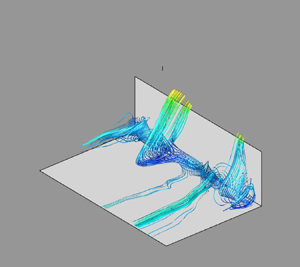
The streamlines of the field corresponding to the superposition of the mean flow and the reconstructed structure $\underline {\varPhi }^{1,C}$ are represented in figure 10 for three different sets of original locations (both forward and backward time integration are performed). Each set of locations consists of a horizontal line along the step face: one close to the inward corner $(x=-0.05, y=0.1)$, one just above the mean recirculation $(x=-0.05, y=0.6)$ and one just above the step edge $(x=-0.05, y=0.9)$. Each type of streamline is associated with the same well-delimited spanwise regions of fluid upstream, illustrating the compactness of the representation. Vizualization of the streaky pattern created by the structure is provided by representing the contour lines of the streamwise velocity in the vertical plane at the step corner $x=0$ in each subplot. Different flow patterns associated with the characteristic structure $\underline {\varPhi }^{1,C}$ can thus be identified.

Figure 10.

Streamlines of the characteristic upstream structure coloured by the streamwise velocity. Streamlines go through the lines $x=-0.1, y=0.1$ (a); $x=-0.05, y=0.6$ (b) and $x=-0.05, y=0.95$ (c). See text for more details.

Near the bottom wall (figure 10a), fluid from the incoming boundary layer gets trapped within the recirculation zone, but then leaves it after a few spins and is ejected over the step. A good agreement is found with experimental (Stuer et al. Reference Stuer, Gyr and Kinzelbach1999) and numerical observations (Fang et al. Reference Fang, Tachie, Bergstrom, Yang and Wang2021, figure 14a). The twisting and ejecting motions from within the recirculation zone are associated with open recirculation streamlines, which cannot be captured by a 2-D representation. Comparison of the incoming streamlines with the lifted-up streamwise velocity contours in the vertical plane at the step corner indicate that the ejected fluid is slower than the mean flow.

At mid-height (figure 10b), flow separation takes place, due to the strong spanwise motions close to the wall. Above the recirculation zone, the flow is collected into different low-speed streaks, which are then ejected over the step. Note that the location of these ejections generally coincides with the fluid leaving the recirculation. Just underneath the step at $y=0.9$ (figure 10c), most of the flow streamlines spread out from upstream locations further away from the wall and are less likely to get trapped in the recirculation zone. As a result, they reach the wall with a higher velocity (as evidenced by the streamwise contour lines in the vertical plane) and without being shifted in the spanwise direction.

4.3. Centrifugal instability

We now investigate the origin of this structure. Due to the presence of the step, the mean flow is characterized by a strong curvature (see figure 3), so that a possible formation mechanism could be a centrifugal instability. A necessary condition for the existence of this instability is given by an inviscid criterion (Drazin & Reid Reference Drazin and Reid1982) based on the Rayleigh discriminant $\varPsi$ that, following Beaudoin et al.'s (Reference Beaudoin, Cadot, Aider and Wesfreid2004) approach for a backward-facing step, can be defined as

(4.4)\begin{equation} \varPsi= \frac{2 U_m \varOmega_z}{R}, \end{equation}

where $U_m^2=U^2+V^2$, $\varOmega _z=\partial V/\partial x - \partial U /\partial y$ and $R$ is the local radius of curvature obtained from Sipp & Jacquin (Reference Sipp and Jacquin2000) as

(4.5)\begin{equation} R = \frac{ (U^2 + V^2)^{3/2}}{U a_y - V a_x}, \end{equation}

where $a_x$ and $a_y$ correspond to the components of the convective acceleration $\underline{U}.\boldsymbol {\nabla } U$. When the Rayleigh discriminant is negative, the flow is potentially unstable to a centrifugal instability. The region where the Rayleigh discriminant is negative with a large modulus is represented in figure 11. It is characterized by two local minima corresponding to the respective local maxima of the streamwise and spanwise velocity fluctuations (see figure 5).

Figure 11.

Contour lines of the Rayleigh discriminant $\varPhi$ – values from $-$0.30 to $-$0.54 with increments of 0.03. The lines are superposed with (a) the time-averaged streamwise velocity component $U$ and (b) the local Görtler number (see text for definition). The region where the Rayleigh discriminant $\varPhi$ is positive is coloured in white.

However, for instability to occur, curvature effects need to overcome the effect of viscosity, a relative measure of which is given by the Görtler number

(4.6)\begin{equation} Go = \frac{U_{fs} \delta^{3/2}}{\nu} {R^{{-}1/2}}, \end{equation}

where in the classical laminar Görtler problem (Saric Reference Saric1994), $\delta$ corresponds to the boundary layer thickness and $U_{fs}$ is the free-stream velocity (here $U_{fs}=1$). Note that although we used a description based on a Görtler number, we did not find any clear evidence of Görtler vortices in the flow. In the present case, the flow is (weakly) turbulent and, as proposed by Tani (Reference Tani1962), the stability characteristics can be determined in a turbulent case if the viscosity is replaced by the turbulent eddy viscosity $\nu _t$, for which we can use Clauser's law $\nu _t \sim 0.018 U \delta _1$. Following Dagaut et al. (Reference Dagaut, Negretti, Balarac and Brun2021), we computed a turbulent Görtler number

(4.7)\begin{equation} Go = \frac{U_{fs} \delta_1^{3/2}}{\nu_t} {R^{{-}1/2}}= \frac{\delta_1^{1/2}}{0.018 R^{1/2}}, \end{equation}

where the displacement thickness $\delta _1$ was estimated at the position of the step in the flat plate turbulent boundary layer.

Figure 11 shows that the upper region close to the step edge is characterized by both a high Görtler number and strongly negative values of the Rayleigh discriminant. Comparison of figure 11 with figure 5 suggests that the region around $x=-0.2$, $y=0.8$, corresponding to the maximum streamwise fluctuation intensity, could be a good candidate for the origin of the instability. An interesting parallel can be drawn with Brès & Colonius's (Reference Brès and Colonius2008) study of the flow over a cavity. Using 3-D linear stability analysis and direct numerical simulation (DNS), they provided evidence of a centrifugal instability mechanism with a spanwise wavelength of the order of the cavity depth for shallow cavities, which is comparable with the dominant wavelengths found upstream of the step.

5.1. Zero spanwise modes

Figure 12 shows that the fluctuating velocity eigenvalues for the spanwise invariant modes $k=0$ are organized in pairs, of the form $2n-1, 2n$ for $n \ge 1$, particularly for the first three couples of modes. The corresponding velocity eigenmodes are represented in figure 13. One can see that they correspond to 2-D, roll-like structures shed from the downstream recirculation bubble. The streamwise component of the modes is important at the location of reattachment, which suggests that the modes could also be associated with the breathing or flapping motion of the separation bubble.

Figure 13.

The POD eigenmodes $\underline {\varPhi }_0^n$; (a,c,e,g) streamwise component $\varPhi _{0}^{n,1}$ and (b,d,f,h) vertical component $\varPhi _0^{n,2}$. The black line represents the contour $\langle U\rangle =0$.

The spectra of the corresponding amplitudes are represented in figure 14. One can see that the range of frequencies covered by the spanwise-averaged velocity is the same for each pair $n$. As we will see below, the organization of the modes into pairs is consistent with convective motion. For the first pair of eigenmodes, two frequencies, one around 0.10 and one around 0.13, can be identified. These values are consistent with the characteristic value of $f x_R/U=0.6$ associated with vortex shedding (Kiya & Sasaki Reference Kiya and Sasaki1983) since we have $x_R=4.3$. For the higher-order pairs, the frequency at 0.10 can still be identified, but the dominant lower-frequency part of the spectrum is characterized by low frequencies while the high-frequency part shifts towards higher frequencies. A peak is observed around $0.03$ in the low-frequency range, which is in good agreement with the non-dimensional flapping frequency of $f x_R/U =0.12$ identified by Kiya & Sasaki (Reference Kiya and Sasaki1983).

Figure 14.

Temporal spectrum of the dominant POD velocity amplitudes $|\hat {a}_{0}^p|^2$, $p \in \{1,\ldots,8\}$.

5.2. Dominant spanwise modes

The dominant wavenumber $k=1$ corresponding to a wavelength $\lambda _z$ of ${\rm \pi}$ is in good agreement with the critical mode of $3$ identified by Lanzerstorfer & Kuhlmann (Reference Lanzerstorfer and Kuhlmann2012) and Wilhelm et al. (Reference Wilhelm, Hartel and Kleiser2003). The first six modes corresponding to this wavenumber are represented in figure 15. The spatial features of the modes are markedly different from those of the 2-D (spanwise invariant) modes: the signature of the shear layer extending above the separation bubble is clear, the modes extend within the recirculation zone and are characterized by a strong spanwise component, which is larger than the vertical component. The modes have different spatial scales: the first three modes are relatively large scale, while modes 4 and 5 are characterized by smaller scales, and mode 6 is characterized by a mixture of large and small scales.

Figure 15.

The POD eigenmodes $Re[\underline {\varPhi }_{1}^n]$. From left to right: streamwise, vertical and spanwise component of the mode. The black line represents the contour $\langle U\rangle =0$.

Figure 16 represents the temporal spectrum of the corresponding amplitudes $a_1^n$. Unlike the upstream region, the modes are characterized by a strong dissymmetry, which is consistent with convective motion, as will be seen in more detail below. The first two modes are characterized by frequencies in the range 0.05–0.15 (in absolute value) with a peak slightly below 0.1, which is also observed for mode 3. However, mode 3 also contains energy in the range $[0.1, 0.25]$, which is also important for mode 4. Mode 5 is characterized by a narrow range of frequencies around 0.22, while mode 6 contains a wide range of frequencies in the range $[0.05, 0.3]$ with a low-frequency peak at 0.05. The overlap in frequency space supports the idea that the modes are physically connected with each other.

Figure 16.

Temporal spectrum of the POD amplitudes $|\hat {a}_1^n|^2$.

5.3. Convection velocity

Comparison of figures 15 and 16 suggests that large scales tend to be associated with low frequencies. However, as shown by Buxton, de Kat & Ganapathisubramani (Reference Buxton, de Kat and Ganapathisubramani2013) in the case of a mixing layer, different scales can be associated with different convection velocities. Convection velocities are typically determined from correlation-based methods (Wills Reference Wills1964). Here, for the mode $k=1$, we use the spatio-temporal splitting induced by POD to infer a convection velocity $C_n$ for each POD mode $n$ as follows.

1. (i) We first extract for each amplitude $a_1^n$ a characteristic frequency $f_{1}^n$ such that

   (5.1)\begin{equation} f_{1}^n= \frac{\displaystyle \sum_{f} |\hat{a}_{1}^n(f)|^2 f }{\displaystyle \sum_f |\hat{a}_{1}^n(f)|^2 }, \end{equation}
   where $f$ spans the space of positive and negative discrete frequencies.

2. (ii) We compute the streamwise Fourier components $\hat {\underline {\varPhi }}_{k}^n(l,y)$ of the spatial mode $\underline {\varPhi }_1^n(x,y)$. It is defined as $\hat {\underline {\varPhi }}_{k}^n(l,y)= \int _{\varOmega _x^{ds}} \underline {\varPhi }_k^n(x,y) \exp (-2 {\rm i} {\rm \pi}l x/L_{\varOmega _x}^{ds})\, {{\rm d}{\kern0.9pt}x}$, where $l$ is the streamwise wavenumber and $\varOmega _x^{ds}=[0,L_{\varOmega _x}^{ds}]$ is the streamwise domain over which the transform is taken. We then extract a characteristic wavenumber $l_m^n$ from

   (5.2)\begin{equation} l_{1}^n= \frac{\displaystyle \sum_{l} \int_1^{y_f} |\hat{\underline{\varPhi}}_{1}^n(l,y)|^2 l\, {{\rm d} y}}{\displaystyle \sum_l \int_1^{y_f} |\hat{\underline{\varPhi}}_{1}^n(l,y)|^2\, {{\rm d} y}}, \end{equation}
   where $l$ spans the space of streamwise wavenumbers. The streamwise Fourier transform was applied to the downstream region $\varOmega _x^{ds}=[0,7]$ over a vertical region $\varOmega _y^{ds}=[1,7]$. End effects due to the non-periodicity of the domain were not found to affect significantly the value of $l_{1}^n$.

3. (iii) The convection velocity for each POD mode is then computed as

   (5.3)\begin{equation} C_1^n = \frac{f_1^n}{l_{1}^n}. \end{equation}

The method described above can be adapted to extract a convection velocity for each pair of spanwise invariant modes, by defining complex modes of the form $\underline {\varPsi }_0^n= \underline {\varPhi }_0^{2n-1} + i \underline {\varPhi }_0^{2n}$, associated with complex amplitudes $z_0^n=a_0^{2n-1} - i a_0^{2n}$, so that

(5.4)\begin{equation} a_0^{2n-1} \underline{\varPhi}_0^{2n-1} + a_0^{2n} \underline{\varPhi}_0^{2n} = Re[ z_0^n \underline{\varPsi}_0^n]. \end{equation}

For the $n$th pair of POD modes $(a_0^{2n-1}, a_0^{2n})$, one then defines a characteristic frequency $f_0^n$ as

(5.5)\begin{equation} f_{0}^n= \frac{\displaystyle \sum_{f} |\hat{z}_{0}^n(f)|^2 f }{\displaystyle \sum_f |\hat{z}_{0}^n(f)|^2}, \end{equation}

and a characteristic streamwise wavenumber $l_0^n$ as

(5.6)\begin{equation} l_{0}^n= \frac{\displaystyle \sum_{l} \int_1^{y_f} |\widehat{\underline{\varPsi}}_{0}^n(l,y)|^2 l\, {{\rm d} y}}{\displaystyle \sum_l \int_1^{y_f} |\widehat{\underline{\varPsi}}_{0}^n(l,y)|^2\, {{\rm d} y} }. \end{equation}

The convection velocity for the $n$th pair is then given by $C_0^n=f_0^n/l_0^n$.

Figure 17 shows the convection velocity for the most energetic POD modes for $k=0$ (a) and $k=1$ (b). For almost all modes, the convection velocity is between 0.5 and 0.7, which is in excellent agreement with results from Largeau & Moriniere (Reference Largeau and Moriniere2007) (0.5–0.62), Camussi et al. (Reference Camussi, Felli, Pereira, Aloisio and Marco2008) (0.4–0.7), Hoarau et al. (Reference Hoarau, Borée, Laumonier and Gervais2006) (0.7), Kiya & Sasaki (Reference Kiya and Sasaki1983) (0.5–0.7). The exception is mode $n=5$ at $k=1$, for which the convection velocity is closer to 1, which suggests that the convective motion there is driven by the external flow. This is consistent with the higher frequencies observed in figure 16, as well as the spatial localization of the mode, which appears to take large values in the external part of the shear layer, further away from the recirculation and from the wall, as evidenced by $\phi _1^{5,1}$ in figure 15.

Figure 17.

Convection velocity for (a) the pair of POD modes $(a_0^{2n-1},a_0^{2n})$ and (b) the modes $a_1^n$. See text for description.

6.1. Global dynamics

We first determine how the spatio-temporal modulations of the backflow regions are connected with the dominant POD modes identified in each region. For the upstream region, figure 20 shows the cross-correlation between the time variations of the volume $V^{up}$ and of the dominant spanwise-averaged fluctuating mode $a_0^{1,up}$. The correlation coefficient between the two curves is $-0.7$ and is maximal in absolute value for a zero time delay. The negative correlation indicates that the recirculation zone grows when the amplitude of the mode decreases, as discussed in § 4. This high correlation is consistent with the relative importance at a zero spanwise wavenumber of the dominant eigenvalue $\lambda _0^{1,up}$ (see figure 6), and shows that the variations of the backflow volume reflect those of the most energetic 2-D fluctuation.

Figure 20.

(a) Cross-correlation between the upstream backflow volume $V^{up}$ and the spanwise-averaged velocity amplitude $a_0^{1,up}$. (b) Cross-correlation between the spatial modulations of the upstream area of the reverse flow $\hat {A}_{k}^{up}$ and the dominant amplitudes of the POD modes in the upstream region $|a_k^{1,up}|^2$.

As was also seen in § 4, a large part of the fluctuation energy is associated with non-zero spanwise wavenumbers. Figure 20 compares for each spanwise wavenumber $k=1$ to $5$, the temporal cross-correlation of the Fourier components of the area of reverse flow $|\hat {A}_{k}^{up}|$ with those of the dominant fluctuations $|a_k^{1,up}|^2$. The maximum correlation is relatively high (in the range 0.5–0.6) for an optimal time delay that is negative and less than one time unit for $k>1$. The physical significance of this time delay is not clear, especially as correlation values remain high at zero time delay. The high correlation indicates that the spatial variations of the upstream recirculation are strongly connected with the most energetic fluctuations in the upstream zone, which confirms the relevance of the characteristic structure identified in § 4.

In the downstream region, as more eigenmodes contribute to the motion at the dominant wavenumbers, the influence of the velocity fluctuations was examined using aggregated contributions $q_k=\sum _{n=1}^{N} E_k^n$, with $E_k^n= \lambda _k^n |a_k^n|^2$ and $N=10$ (which represents about 50 % of the kinetic energy at this wavenumber). The cross-correlation between these aggregated contributions and the downstream backflow volume $V^{ds}$ is shown in figure 21. No significant correlation was observed for the spanwise invariant modes, which can be expected in view of their low contribution to the fluctuations in the downstream recirculation. In contrast, a significant negative correlation ($-0.49$) was obtained for the dominant first wavenumber. The maximal anti-correlation reached $-0.7$ when higher spanwise wavenumbers were included (up to $k=9$), which confirms the importance of the lowest mode $k=1$. The optimal time delays were small, i.e. of the order of 1–2 time units, and negative. Although it may be difficult to interpret these time delays, the fact that they are negative is consistent with the idea that the downstream separation zone is influenced by the development of the shear layer above it as well as the dominant POD modes at $k=1$ that characterize it.

Figure 21.

Correlation between the temporal variations of the downstream backflow volume $V^{ds}$ and the amplitudes of the global POD modes.

We also computed various cross-correlations between the upstream fluctuations and the downstream backflow area (not shown). No correlation larger than 0.25 in absolute value was obtained. This points to a significant reorganization of the flow past the edge of the step, which we attempt to track using local indicators in the next section.

6.2. Local dynamics at the edge

We now discuss the connection between the upstream velocity fluctuations and the downstream recirculation with a focus on the dynamics at the edge of the step. Figure 22 shows, for two different instants $t_{min}$ and $t_{max}$, a horizontal and a vertical section of the streamwise velocity field respectively located upstream of the step at a height of $y=0.9$ and directly downstream of the edge at $x=0.02$ (the sections are represented in figure 23a). The two instants correspond to the times $t_{min}$ and $t_{max}$ for which the downstream backflow volume $V^{ds}$ is respectively minimal and maximal. For both times, the streamwise velocity is organized into a similar streaky pattern that persists from the horizontal to the vertical plane. However, the streaks are more intense when the volume of reverse flow is maximal: the plane-averaged backflow in the horizontal plane at $t_{max}$ is larger by 70 %, and its maximum value is more than twice as high than at $t_{min}$, while the vertical extent of the most intense streaks in the vertical plane at $t_{max}$ is higher, and can reach above the recirculation height (0.25). This suggests that the downstream separation zone is influenced by the incoming flow and, in particular, the streaks associated with ejections of low-speed fluid at the step edge.

Figure 22.

Instantaneous streamwise velocity in the vertical (a,b) and horizontal (c,d) planes respectively indicated in dark blue and bright green in figure 23. (a,c) Time at which the downstream backflow volume $V^{ds}$ is minimum, (b,d) time at which the downstream backflow volume $V^{ds}$ is maximum.

Figure 23.

(a) Position of the two section planes represented in figure 22 at $y=0.9$ and $x=0.01$. (b) Top: evolution of the maximum principal stretching eigenvalue $\lambda _S^{max}$ in the plane $x=0.01$ (see text for definition). Bottom: evolution of the momentum injected at the edge $M_e^{1/2}$ along the line $(x=-0.02, y=1)$. The dashed lines correspond to the time-averaged values.

A quantity of interest to characterize instantaneous upstream dynamics is therefore the spanwise-averaged flux of streamwise velocity that crosses the plane $y=1$ at the edge, a measure of which is given by the momentum deficit

(6.6)\begin{equation} - M_e={-}\frac{1}{L_z}\int_0^{L_z}[uv](x={-}e,y=1,z)\, {\rm d} z \quad \textrm{where } e =0.02. \end{equation}

A local characteristic time scale $\tau ^{up}$ for the ejection process can be built from the velocity scale $U_e=M_e^{1/2}$ and a characteristic distance $d^{up}$, which should be a fraction of the step height and can be tentatively estimated as $d^{up} \approx 0.2-0.4$, based on the location of the fluctuation peaks. This yields

(6.7)\begin{equation} \tau^{up} = \frac{d^{up}}{M_e^{1/2}} \quad \textrm{with } d^{up} \approx 0.3. \end{equation}

Downstream of the step, the development of perturbations in the shear layer should occur on a time scale $\tau ^{ds}$ that varies like $1/\delta _{\omega }$, where $\delta _{\omega }$ is a characteristic length scale. From Ho & Huerre (Reference Ho and Huerre1984), the initial maximal spatial growth rate of the shear layer instability is of the order of $0.12 / \delta _{S}$ where $\delta _{S}$ is the shear layer thickness, so that $\delta _{\omega } \sim C^{ds} \delta _{S}$ with $C^{ds}=1/0.12 \approx 8$. A measure of the shear layer thickness $\delta _{S}$ can be obtained from the inverse of the largest positive eigenvalue $\lambda _S$ of the mean strain rate $\frac {1}{2}(\boldsymbol {\nabla } \underline {U} + \boldsymbol {\nabla } \underline {U}^T)$, which was used by Fang et al. (Reference Fang, Tachie, Bergstrom, Yang and Wang2021) to track the position of the shear layer. In a similar fashion, we define an instantaneous shear layer thickness based on the maximal value of the largest positive eigenvalue of the spanwise-averaged strain rate in the vertical plane directly downstream of the edge:

(6.8)\begin{equation} \lambda_S^{max}(t) = \mathrm{max}_{y} \lambda_S(x=0.01,y,t). \end{equation}

The time-averaged location of the maximum corresponds to a vertical distance of $y=0.02$ above the edge. The local time scale at the edge of the shear layer $\tau ^{ds}$ can therefore be estimated as

(6.9)\begin{equation} \tau^{ds} = \frac{1}{\delta_{\omega}}=\frac{C^{ds}}{\delta_S} \sim \frac{C^{ds}}{\lambda_S^{max}} \quad \textrm{with } C^{ds} \sim 8. \end{equation}

Figure 23 compares the time evolution of the characteristic velocity for the ejection process $U_e=M_e^{1/2}$ with the shear layer time scale $\lambda _S^{max}$. Both signals are almost perfectly correlated with a correlation coefficient of $0.95$. We point out that we computed several other correlation coefficients based on the spanwise-averaged velocity, such as that between the wall shear and $M_e$, as well as that between $\lambda _S^{max}$ and the velocity modulus. All coefficients were significantly inferior to the 0.95 value, which means that the match does not simply reflect the fact that the two signals $M_e$ and $\lambda _S^{max}$ are based on the spanwise-averaged velocity measured at two nearby locations. In addition, both signals have nearly the same root mean square to mean value, which suggests that they are directly proportional to each other, with a ratio $\langle \lambda _S^{max}\rangle /\langle M_e^{1/2}\rangle$ of about 60. This leads to a ratio for $\tau ^{up}/\tau ^{ds}$ of about $60 d^{up}/C^{ds} \approx 2.25$, which is sufficiently close to 1 for $\tau ^{up}$ and $\tau ^{ds}$ to be considered of the same order, given the crudeness of our estimates. This suggests that the shear layer dynamics instantaneously adapt to the upstream ejections, so that a decrease in ejections will immediately trigger a faster development of the shear layer perturbations. A direct connection is therefore established between the momentum deficit associated with the ejections and the strength of the shear layer downstream of the step.

To get a better understanding of this connection, we define an extended correlation coefficient to measure the cross-correlation between the complex Fourier amplitudes of the momentum deficit $-\hat {M}_{e,k}$ and those of the backflow areas $\hat {A}_{k}^{\alpha }$ with $\alpha \in \{up, ds\}$. Since $M_e$ is a small-scale, highly intermittent quantity, the signals were time filtered using a moving average of $5$ convective time units corresponding to less than one characteristic shedding time. The extended correlation coefficient $\bar {C}$ is defined as

(6.10)\begin{equation} \bar{C}(q_1,q_2)=\frac{Re[\langle (\overline{q_1}-\langle q_1\rangle) (\overline{q_2}-\langle q_2\rangle )*\rangle ]}{\overline{|q_1|}^{rms}\overline{|q_2|}^{rms}}, \end{equation}

where $\bar {q}$ represents the time-filtered version of $q$, $\langle q\rangle$ its time average and $|\bar {q}|^{rms}$ the standard deviation of its filtered modulus. Results are presented in figure 24 for the upstream recirculation (a) and the downstream recirculation (b). For Fourier modes $1 \le k \le 5$, the correlation between $-\hat {M}_{e,k}$ and the upstream recirculation is strong – larger than $0.6$ – with optimal time delays inferior to one time unit (a slightly larger time delay of 3 units is observed for the less energetic mode $k=1$). This shows that the modulations of the recirculation at the bottom of the step are directly connected with the ejections at the edge, and that both match the variations of the characteristic structure identified in § 4.

Figure 24.

Cross-correlation $\bar {C}$ between the spanwise Fourier components of the upstream (a) and downstream (b) areas of the reverse flow $\hat {A}_k$ and those of the momentum deficit $-\hat {M}_{e,k}$. The signals are filtered with a moving average of 5 time units. See text for a definition of $\bar {C}$.

It is interesting to contrast these results with those obtained for the downstream recirculation. Only the spanwise-averaged area (or volume) of reverse flow $V^{ds}$ is well correlated – with a correlation coefficient larger than $0.6$ – with the average momentum deficit $-\hat {M}_{e,0}$, indicating that an increase in momentum deficit at the edge of the step results in a larger recirculation downstream. The corresponding optimal time delay was positive and of the order of $2$ convective time units. Interestingly, no such correlation was detected for higher modes, which confirms a fast reorganization of the flow downstream of the step (and was also substantiated by examination of instantaneous fields).

We therefore propose the following description, summarized in figure 25: low-speed fluid is entrained into the upstream recirculation bubble and ejected with a strong spanwise motion into low-velocity streaks over the edge of the step. The global momentum deficit due to these local ejections impacts the development of the shear layer and the downstream recirculation, although the fluctuations are quickly reorganized. A higher ejection rate (low $M_e$) leads to a weaker development of the shear layer and a larger recirculation zone. The flow in the shear layer is characterized by a low spanwise modulation, but becomes more two dimensional downstream of the reattachment.

Figure 25.

Sketch of the dynamics of the forward-facing step.

7.1. The POD-based models

In this section we propose a model to reconstruct the dynamics of the most energetic POD modes, which are characterized by a range of low frequencies. The model is based on a simplified version of the POD-based models obtained by projection of the Navier–Stokes equations onto the basis of the spatial POD modes. The construction of dynamical systems to predict the amplitudes of the POD modes was first proposed by Aubry et al. (Reference Aubry, Holmes, Lumley and Stone1988) and a thorough discussion can be found in Holmes et al. (Reference Holmes, Lumley and Berkooz1996).

Its general form for the set of normalized amplitudes $a_k^n$ with $k \in \{-K, \ldots K\}$ and $n \in \{1, \ldots N_T\}$ can be given as

(7.1)\begin{equation} \dot{a}_k^n = A_k^{nm} a_k^m + Q_{kk'}^{nmp} a_k^m a_{k-k'}^p + T_k^n, \end{equation}

where Einstein notation has been used.

The linear component $A_k^{nm}$ can be further decomposed as

(7.2)\begin{equation} A_k^{nm} = D_k^{nm} + L_k^{nm}, \end{equation}

where $D_k^{nm}$ corresponds to the diffusion term

(7.3)\begin{equation} D_k^{nm} = \frac{1}{Re} \sqrt{\frac{\lambda_k^m}{\lambda_k^n}} \iint \phi_k^{n,i*} \left({-}k_z^2 + \frac{\partial^2 }{\partial x^2} + \frac{\partial^2 }{\partial y^2} \right)\phi_k^{m,i}\, {{\rm d}{\kern0.9pt}x}\, {{\rm d} y}, \end{equation}

and $L_k^{nm}$ represents the interaction with the mean mode

(7.4)\begin{equation} L_k^{nm}={-} \sqrt{\frac{\lambda_k^m}{\lambda_k^n}}\iint \left( \phi_k^{n,i*} U_j \frac{\partial \phi_{k}^{m,i}}{\partial x_j} + \phi_k^{n,i*} \phi_{k}^{j,m} \frac{\partial U_i}{\partial x_j} \right)\, {{\rm d}{\kern0.9pt}x}\, {{\rm d} y}. \end{equation}

We denote by $Q_{kk'}^{nmp}$ the interaction coefficient due to the nonlinear term $\underline {q} . \boldsymbol {\nabla } \underline {q}$ in the Navier–Stokes equations ($\underline {q} . \boldsymbol {\nabla } \underline {q}$ represents the velocity fluctuation). It can also include the effect of the pressure gradient if it is not neglected (see Noack, Papas & Monkewitz Reference Noack, Papas and Monkewitz2005).

We denote by $T_k^n$ the effect of the modes that are excluded from the truncation

(7.5)\begin{equation} T_k^{n} = \int \hat{\tau}_k^i \phi_k^{m,i*}\, {{\rm d}{\kern0.9pt}x}\, {{\rm d} y} - Q_{kk'}^{nmp} a_k^m a_{k-k'}^p, \end{equation}

where $\hat {\tau }_k^i$ is the Fourier transform of $q_j ({\partial q_i}/{\partial x_j})$.

Here $T_k^{n}$ is similar to a subgrid-scale stress term that needs to be modelled with additional assumptions in order to close the equations. The most general form is to assume that

(7.6)\begin{equation} T_k^{n} = \alpha_k^n D_k^{nm} a_{km},\end{equation}

where $\alpha _k^n$ is a function that is equivalent to a turbulent eddy viscosity $\nu _t/\nu$. In early derivations of the model, $\alpha _k^n$ was assumed to be constant (Aubry et al. Reference Aubry, Holmes, Lumley and Stone1988) but in more recent implementations (see, for instance, Podvin et al. Reference Podvin, Pellerin, Fraigneau, Bonnavion and Cadot2021), $\alpha _k$ can be a nonlinear function of the resolved modes $a_k^n$. Following Osth et al. (Reference Osth, Noack, Krajnoci, Borée and Barros2014), the turbulent eddy viscosity is assumed to scale with the characteristic velocity of the resolved modes $\sqrt {\sum _{m=1}^{N_T} |a_k^m|^2}$, which can be expanded into a sum of a constant term and a quadratic term $1/2 \sum _{m=1}^{N_T} (\lambda _k^m + |a_k^m|^2)$ (Podvin & Sergent Reference Podvin and Sergent2017). The proportionality constant is negative so that the effect of $T_k^n$ is to prevent the unphysical growth of fluctuations in the model.

7.2. Linear model

We derive a linearized version of the model for the most energetic POD modes $a_k^n$, with $k=0,1$ and $n \le 10$. The linear model is based on the assumption that the driving mechanism for the fluctuations is their direct interaction with the mean flow – through convection and deformation by the mean shear. Some justification for this can be found on the large separation between the intensity of the mean velocity and that of the fluctuations (the largest POD eigenvalue is less than 1 %). We therefore assume that the quadratic interaction terms $Q$, the effect of which is to redistribute energy among the resolved modes, can be neglected.

A second assumption is that the effect of both molecular ($D$) and turbulent ($T$) viscosity is also small and is limited to preventing non-physical unbounded growth of the fluctuations without modifying their characteristic frequencies. Figure 26 (top row) shows the spectrum of the matrix $L_0$ and $L_1$ for a truncation of 10 modes. Each eigenvalue $\mu _k^n$ has a small positive real part, which is much smaller than its imaginary part $\mu _k^n = \mathrm {Re}[\mu _k^n]+ {\rm i}\, \mathrm {Im}[\mu _k^n]$ with $\mathrm {Re}[\mu _k^n] \ll |\mathrm {Im}[\mu _k^n]|$ (the fact that the real part is positive is physically consistent with the fact that the fluctuations are extracting energy from the mean flow). Figure 26 (bottom row) shows the values of the matrix $D_k$ for the wavenumber $k=1$ (a similar behaviour was observed for $k=0$). We can see that $D_1$ is essentially diagonal. Its values $D_1^{nn}$ are mostly real and negative, and their relatively small magnitudes increase only slightly with $n$. Therefore, $D_k$ can be considered roughly proportional to the identity matrix as a first approximation,

(7.7)\begin{equation} D_k \approx{-}\eta_k I, \quad \textrm{with } 0 < \eta_k \ll 1. \end{equation}

This means that $L_k+D_k$ can be assumed to diagonalize in the same basis $B$ as $L$ with eigenvalues $\mu _k^n - \eta _k = \mathrm {Re}[\mu _k^n] - \eta _k + {\rm i}\, \mathrm {Im}[\mu _k^n]$.

Figure 26.

(a,b) Eigenvalues of $L_k$ for a ten-mode truncation for $k=0$ (a) and $k=1$ (b). (c,d) Dissipation matrix $D_1$ real part (c) and imaginary part (d).

Since the closure for the unresolved stresses $T_k$ is based on the properties of the dissipation matrix $D_k$ (7.6), we can further assume that the additional effect of the unresolved stresses is to merely modify the real part of the eigenvalues, with $| {\rm Re}[\mu _k^n] - \eta _k ( 1 + \mathrm {Sup}_p \alpha _k^p) | \ll {\rm Im}[\mu _k^n]$. Equation (7.1) can then be approximated as

(7.8)\begin{equation} \dot{a}_k^n = (L_k^{nm} + (1 + \alpha_k^n)D_k^{nm} ) a_k^m \approx \tilde{L}_k^{nm} a_k^m, \end{equation}

where $\tilde {L}_k$ diagonalizes in the same basis $B$ as $L_k$ with purely imaginary eigenvalues ${\rm i}\, \mathrm {Im}[\mu _k^n]$:

(7.9)\begin{equation} \tilde{L}_k = B \begin{bmatrix} {\rm i}\,\mathrm{Im}[\mu_k^1] & 0 & \ldots \\ 0 & {\rm i}\, \mathrm{Im}[\mu_k^2] & \ldots \\ \ldots & \ldots & {\rm i}\, \mathrm{Im}[\mu_k^{N_T}] \end{bmatrix} B^{{-}1}. \end{equation}

The $n$th column of the matrix $B$ contains the eigenvector $b_k^n$ associated with the eigenvalue ${\rm i}\, {\rm Im}[\mu _k^n]$ and expressed in the basis $a_k^n$. Conversely, each POD amplitude $a_k^n$ can be represented as a sum of eigenmodes $b_k^p: a_k^n = \sum _{p=1}^{N_{T}} \beta _k^{np} b_k^p$. Predicted amplitudes for the model can then be reconstructed using

(7.10)\begin{equation} a_k^{n,pred}(t) = \beta_k^{np}\, {\rm e}^{{\rm i} \,\mathrm{Im}[ \mu_k^{p}] t}. \end{equation}

Figure 27 compares the spectra of the POD amplitudes extracted from the DNS with the frequencies obtained by considering $N_T=10$ and $N_T=6$ systems for $k=0$ and $k=1$. The predicted spectra shown for each mode $n$ are arbitrarily rescaled by $\mathrm {Max}_p \beta _{np}/\mathrm {Max}_f |\hat {a}_k^n(f)|$ for comparison purposes. We see that in all cases, the prediction provides a good identification of the dominant frequencies of the amplitude spectra, which supports the assumption of the fundamentally linear nature of the dynamics. We emphasize that the model frequencies are solely determined from the spatial modes extracted from the sampled autocorrelation tensor, independently of the sampling rate used to compute the tensor.

Figure 27.

Predicted frequencies of the dominant POD amplitudes with the linear autonomous model (LM) for two different truncations $N_T=6$ (black lines) and $N_T=10$ (red lines): (a) $|\hat {a}_{0}^n|^2$ for $n \in \{1, \ldots 6\}$ and (b) $|\hat {a}_{1}^n|^2 n \in \{1, \ldots 6\}$.

7.3. Time-varying linear model

Unlike those of the DNS, the spectra shown in figure 27 are discrete and limited to $N_T$ frequencies, since the linear model has constant coefficients. To make the model more physical, we modify the model so that the strength of the mean mode is allowed to vary in time. As a first approximation, we assume that this variation is solely driven by the local time fluctuations of the mean shear at the edge, which is determined by the maximum stretching eigenvalue $\lambda _S^{max}$ and, therefore, the ejections over the edge (as evidenced in figure 23). The modified model will be called the forced model.

If $\epsilon$ is the time-dependent modulation of the shear layer $\epsilon = \lambda _S^{max}/ \langle \lambda _S^{max}\rangle - 1$, the forced model is defined as

(7.11)\begin{equation} \dot{a}_k^n = \tilde{L}_k^{nm} ( 1 + \epsilon ) a_k^m. \end{equation}

For all wavenumbers, the model was integrated from the initial condition $a_k^n=1$. Using arbitrary initial phases between the modes did not affect the general characteristics reported below. Figures 28(a) and 28(b) show the spectra of the forced model for the modes $k=0$ and $k=1$, which can be respectively compared with figures 14 and 16. Although complete agreement should not be expected given the crudeness of our assumption, it can be seen that the model roughly reproduces the widths and heights of the spectral bands of $a_k^n$ observed in the DNS. Figures 28(c) and 28(d) compare the probability distribution functions of the amplitude moduli $|a_k^n|$ for $k=0$ and $k=1$ in the DNS, the linear and the forced models. Although some discrepancies are occasionally observed in the distribution tails, both models capture equally well the shape of the distributions, which are characterized by frequent low values for the spanwise invariant modes and a non-zero maximum around 0.5–1 for the spanwise modes.

Figure 28.

(a) Predicted spectrum of the dominant POD amplitudes $|\hat {a}_{0}^n|^2$ with the forced model (FM). (b) Predicted spectrum of the dominant POD amplitudes $|\hat {a}_{1}^n|^2$. (c) Histograms of the amplitude moduli $|a_0^n|$, $n \in \{1, 8\}$ for the DNS, linear model (LM) and FM. (d) Histograms of the amplitude moduli $|a_1^n|$, $n \in \{1, 6\}$ for the DNS, LM and FM.